The apparent tail of the Galactic center object G2/DSO

Abstract

The observations of the near-infrared excess object G2/DSO induced an increased attention towards the Galactic center and its vicinity. The predicted flaring event in 2014 and the outcome of the intense monitoring of the supermassive black hole in the center of our Galaxy did not fulfill all predictions about a significantly enhanced accretion event. Subsequent observations furthermore addressed the question concerning the nature of the object because of its compact shape, especially during its periapse in 2014. Theoretical approaches have attempted to answer the contradicting behavior of the object, resisting the expected dissolution of a gaseous cloud due to tidal forces in combination with evaporation and hydrodynamical instabilities. However, assuming that the object is rather a dust-enshrouded young stellar object seems to be in line with the predictions of several groups and observations presented in numerous publications. Here we present a detailed overview and analysis of the observations of the object that have been performed with SINFONI (VLT) and provide a comprehensive approach to clarify the nature of G2/DSO. We show that the tail emission consists of two isolated and compact sources with different orbital elements for each source rather than an extended and stretched component as it appeared in previous representations of the same data. Considering our recent publications, we propose that the monitored dust-enshrouded objects are remnants of a dissolved young stellar cluster whose formation was initiated in the Circum-nuclear Disk. This indicates a shared history which agrees with our analysis of the D- and X-sources.

1 Introduction

Observations of the direct vicinity of the supermassive black hole Sgr A* in the center of our Galaxy have been bringing unexpected findings. For instance, the S-cluster with a projected diameter of about 40 mpc around Sgr A* harbors young stars, predominantly of B-type spectral class. The origin of the related S-stars and the question, where they have formed, is still unresolved (Morris & Serabyn, 1996; Ghez et al., 2003). Several publications aim to answer the two possible scenarios, namely, whether the in-situ star formation (SF) or dynamical-segregation processes lead to the presence of young early-type stars (see, e.g., Nayakshin et al., 2007; Jalali et al., 2014; Moser et al., 2017) that form a cusp-like surface-brightness density distribution. Another example demonstrating that the Galactic center (GC) is a unique dynamical laboratory is the recent outcome of Ali et al. (2020) where the authors find a non-randomized distribution of the S-stars, quite contrary to the earlier results. The stellar members belong to a multi-disk arrangement that shapes the S-cluster. On even smaller scales (< 6 mpc), the observation with GRAVITY of the pericenter passage of S2 (Schödel et al., 2002) in 2018 confirmed the Schwarzschild procession (Gravity Collaboration et al., 2018; Do et al., 2019a), which was tentatively investigated by Parsa et al. (2017). Recently, Fragione & Loeb (2020) used the orbital parameters of the newly discovered S-cluster members S4711-S4715 and S62 (Gillessen et al., 2009; Peißker et al., 2020a, d) to derive an upper limit for the spin of Sgr A*.
However, not only does the analysis of stellar orbits reveal details about the nature of the SMBH and its environment (Zajacek & Tursunov, 2019; Zajaček et al., 2020; Hosseini et al., 2020). Because a part of the GC data is gathered through the Integral Field Unit (IFU) of the Spectrograph for INtegral Field Observations in the Near Infrared (SINFONI) mounted at the Very Large Telescope (VLT), it is possible to access several emission lines in the near-infrared (NIR) (Eisenhauer et al., 2003; Bonnet et al., 2004). With this information, it is possible to reveal, for example, large scale structures, such as the prominent Br$\gamma$-bar (Schödel et al., 2010; Peißker et al., 2020c). Furthermore, Doppler-shifted lines, which represent the line-of-sight (LOS) velocity of gas that is dynamically detached from the background and foreground stationary medium, can be detected. Herewith, Gillessen et al. (2012) reported the observation of a $\approx\,3\,M_{\oplus}$ gas cloud (and its tail) that had been detected in the red-shifted Br$\gamma$ regime. The cloud moved on a highly eccentric Keplerian orbit towards Sgr A*. According to Gillessen et al. (2012), the cloud G2 (named by Burkert et al., 2012) was expected to be tidally stretched before and during its pericenter passage. The same authors furthermore predicted that the cloud gets destroyed when it encounters the hot atmosphere surrounding Sgr A* due to the combined effect of the tidal stretching, evaporation due to heat conduction, and the quick development of hydrodynamical instabilities. Therefore, the material of the destroyed cloud was supposed to enrich the accretion depot of the SMBH. As a consequence, such a tidal process should have resulted in an enhanced accretion activity of Sgr A*, which would be manifested by an increased NIR and X-ray flare activity or a “firework" as underlined by the the authors. Every attempt to observe the predicted increased flaring activity of Sgr A*, however, failed. The clockwise stellar disk of massive OB/Wolf-Rayet stars (Paumard et al., 2006) was supposed to serve as a birth place for the cloud (Burkert et al., 2012). It was claimed, that shocked winds of the stellar members of the clockwise disk with velocities up to 1000 km/s create hot plasma that is attracted by Sgr A* (and consequently interpreted as G2).
Furthermore, Gillessen et al. (2019) reported the detection of a drag force acting on G2 to explain the orbital motion of the compact object on a bound trajectory which was claimed to deviate from the Keplerian orbit. While Gillessen et al. (2012) and Gillessen et al. (2019) pursue a core-less gaseous cloud model, Murray-Clay & Loeb (2012) interpret the findings using the model of a low-mass star surrounded by a protoplanetary disk. Also, other authors agree that the observed characteristics of G2 are more consistent with a stellar source that is embedded in a dense gaseous-dusty envelope (see selected references like, e.g., Eckart et al., 2013; Scoville & Burkert, 2013; Zajaček et al., 2014; Witzel et al., 2014; Valencia-S. et al., 2015; Prodan et al., 2015; Shahzamanian et al., 2016; Stephan et al., 2016; Kohler, 2017). Lately, Peißker et al. (2020b) presented a multiwavelength analysis of G2 where the authors use the name Dusty S-cluster Object (DSO) for G2 to underline the dusty nature of the source, in particular its prominent near-infrared excess that is related to the effective blackbody temperature of $\sim 500\,{\rm K}$ (see also Eckart et al., 2013). In contrast, many publications find no K-band counterpart of G2 (e.g. Gillessen et al., 2012; Pfuhl et al., 2015; Plewa et al., 2017; Ciurlo et al., 2020).To reflect the disputed nature of the source, we adapt the name G2/DSO throughout the manuscript. The overall spectral energy distribution (SED) that corresponds to the continuum emission of the G2/DSO in the H-, K-, L-, and M-bands as presented in Peißker et al. (2020b) is based on a two-component fit, which corresponds to the star–envelope system. This analysis emphasizes the nature of the G2/DSO as a young stellar object (hereafter YSO) that is embedded in a dense gaseous-dusty envelope.
This interpretation seems to be in agreement with the analysis of G1, a predecessor of G2/DSO (see Pfuhl et al., 2015). The G1 object, found by Clénet et al. (2005), was originally classified as a gas cloud. Pfuhl et al. (2015) connected the orbit of G1 and G2/DSO to claim that both sources are part of a common gaseous streamer. The authors propose that G1 and G2/DSO share similar orbits. Hence, G2/DSO should follow the trajectory of the cloud G1. However, recent observations presented by Witzel et al. (2017) do not support this scenario since the orbits of these objects differ substantially. Furthermore, it seems that several other objects (10+) share a similar dynamical history (Ciurlo et al., 2020; Peißker et al., 2020b), potentially forming a unique population within the S cluster. For some of these sources that are mainly found in the Doppler-shifted Br$\gamma$ regime, a K-band continuum-emission counterpart can be detected indicating a stellar nature (see, for example, X7 or G2/DSO as presented in Peißker et al., 2020b). Also, the sources of the D-complex (Peißker et al., 2020b) imply a common origin which seem to support the in-situ star forming scenario (for simulations, see also Jalali et al., 2014).
In this work, we will investigate the G2/DSO source in detail. Since we use high-pass filter and avoid Gaussian smoothing for the here presented data, we present a new orbital solution based on SINFONI data covering 2005-2019. We will underline the orbital analysis with related Br$\gamma$ line maps that are accompanied by K-band continuum detections of G2/DSO. Additionally, we compare position-position-velocity maps with the literature. Based on the analysis, we introduce new sources that are following the G2/DSO source that we call Obedient Star 1 and 2 (OS1 and OS2).
In Section 2, we will introduce the used data and explain the applied analyzing tools. In Section 3, we will show the G2/DSO with its Keplerian orbit around Sgr A* and the detection of the newly discovered sources OS1 and OS2. The discussion part in Section 4 is followed by the final conclusion.
For a comprehensive list of the here used data, please consider Appendix A.

2 Data and Analysis

Here we explain the data accumulation, the instrument settings, and the applied analysis tools.

2.1 SINFONI and the VLT

SINFONI was previously mounted at the unit telescope (UT) 4 (VLT), afterwards it was relocated to UT3 (VLT). It is now decommissioned. The instrument uses a slicer to create pseudo longslits. Then, a spectral dispersion creates groups of wavelength-dependent longslits. After this process, a 3d data cube is reconstructed with 2 spatial dimensions and 1 spectral dimension. For a fraction of the data, a laser guide star (LGS) was used. Since UT3 does not support LGS-guidance, the data that were observed after the relocation used exclusively a natural guide star (NGS). Typically, this NGS is located $15".54$ north and $8".85$ south of Sgr A*. Since SINFONI uses an optical wavefront sensor, the selection of possible bright (14-15 mag) NGS-sources is limited. The location of the bright radio source Sgr A*, which can be associated with the SMBH (see Eckart et al., 2002, 2017), can be found at Right Ascension (RA) $17:45:40.05$ and Declination (DEC) $-29^{\circ}\,00^{\prime}\,28.120"$ (J2000). In the following subsections, we will explain the procedure of deriving the position of Sgr A* in the individual data cubes. In Appendix A, we list the investigated SINFONI cubes including the quality, exposure time of the individual observations, the related IDs, and the publications where we already used the data.

2.2 Dataset and instrument settings

For the observations, the smallest available plate scale was used (12.5 mas) and the wavelength range was set to the H+K-band ($1.45\,\mu m\,-\,2.45\,\mu m$). The exposure time for a single data cube was set between 400 and 600 seconds. We use the standard object-sky-object nod cadence. With that, the sky corrections can be applied to the individual data cubes. Because of the background noise and the small field of view (FOV) of $0.8\,\times\,0.8$ arcsec, the GC/S-cluster observations are dithered around the position of Sgr A* or S2. After the usual reduction steps that are applied with the ESO pipeline (Modigliani et al., 2007), the single data cubes of several nights (see Appendix A for the used data) are stacked to create a mosaic for each year between 2005 and 2019 with a higher signal-to-noise (S/N) ratio but also an increased FOV. Furthermore, the SINFONI pipeline automatically applies a barycentric and heliocentric correction.

2.3 The position of Sgr A*

From the well-observed orbit of the brightest (in K-band) S-cluster member S2 (see, e.g., Parsa et al., 2017; Ali et al., 2020), we derive the position of Sgr A* with an uncertainty of less than 12.5 mas. This uncertainty already contains a linear transformation but also corrections for a distorted FOV. While this is applied in a satisfying procedure for the data discussed in Parsa et al. (2017) and Ali et al. (2020), the SINFONI data suffers from image motion as a function of wavelength. While this effect is certainly suppressed in single-band observations, the H+K-band observations with SINFONI do show a non-negligible movement of the stars between the H- and K-band. For example, the position of S2 does change by over 1 pixel (= 12.5 mas) by comparing individual line maps. While Jia et al. (2019) addresses some of the GC observation problems for the KECK telescope that can also be applied to the VLT data (stellar confusion, variable PSF, artifical PSF-wing sources), we do not agree with the 1 mas uncertainty given by Gillessen et al. (2017). This underestimates general crowding problems (for example, blend stars, see Sabha et al., 2012) and does not reflect the noise character of the SINFONI data. As pointed out by the SINFONI manual, the shape and intensity of the point spread function is a function of the source position on the detector. This results in unaccurate positions of stellar sources. Furthermore, Eisenhauer et al. (2003) discussed the issue of image motion for high-exposure observations (above several hours). Since this effect is nonlinear and depends on the total integration time as well as the weather conditions, we will adapt a conservative uncertainty of 12.5 mas for the position of Sgr A* in the SINFONI data. In the following, we will elaborate on this issue in more detail.

2.3.1 Image motion of SINFONI long time exposures

As mentioned by Eisenhauer et al. (2003), short-time exposures do not suffer from image motion (i.e. the apparent movement of a source as a function of wavelength and hence channel). Unfortunately, the image motion of SINFONI is not broadly covered by the literature. Hence, we will investigate this effect with the available GC data. We randomly pick 5 single exposures with integration times of $\geq\,400$ sec. Furthermore, we will compare the image motion of single exposures and final mosaics. We note that the image motion only appears in the horizontal direction.

ID	Date	DIT	x1	x2	$\Delta$x
		[sec]	[px]	[px]	[px]
081.B-0568(A)	06.04.2008	600	38.756	35.404	-3.352
087.B-0117(I)	02.05.2011	600	22.421	23.518	1.097
093.B-0932(A)	03.04.2014	400	45.155	45.143	-0.012
594.B-0498(R)	14.04.2016	600	37.742	38.2538	0.511
091.B-0183(H)	26.03.2018	600	49.592	47.595	-1.997

Table 1: Image motion of S2 for randomly picked SINFONI exposures. For every item, we use the channel 385 (x₁) and 1985 (x₂), which covers a wavelength range between $1.6\,\mu m\,-\,2.4\,\mu m$. We use a Gaussian with a Kernel of 5 pixels to extract the related positions. The usual positioning uncertainty is of the order of about $1\,-\,2\,\%$.

In Table 1, we list a few exemplary exposures. However, this nonlinear image motion can be observed in every single observation. The effect increases with the exposure time. Since a technical discussion is beyond the scope of this work, we will categorize the image motion as a sporadic statistical behavior of the data. Hence, the more single exposures are combined, the more the image motion decreases.

Final mosaic	Total Exp	x1	x2	$\Delta$x
		[px]	[px]	[px]
2008	21	51.125	50.513	0.612
2011	43	51.618	51.103	0.515
2014	310	60.187	59.765	0.422
2016	60	61.822	60.587	1.235
2018	114	61.237	60.832	0.405

Table 2: Image motion of S2 for the final mosaics that are a combination of several single exposures. We use the same approach as for the listed cubes in Tab. 1.

While the image motion of a single exposure is an unavoidable mandatory condition, it can efficiently be decreased by combining many data cubes to a final mosaic (see Table 2). As mentioned before, the effect is the most profound for sources in the center of the FOV (here: S2). For objects at the border of the data cube, the effect differs by $1\,-\,20\,\%$. For example, the S-cluster star S4 (see Fig. 2) in 2016 moves by $\Delta x_{S4}\,=\,0.112$ px while S2 shows a difference of $\Delta x_{S2}\,=\,1.235$ px (see Table 2).
The outcome of the example is expected since the SINFONI manual states that the shape of a PSF differs depending on the position on the CCD chip. This may not influence the observation of a single source but does impact the analysis of a crowded field like the GC.

2.4 Line maps

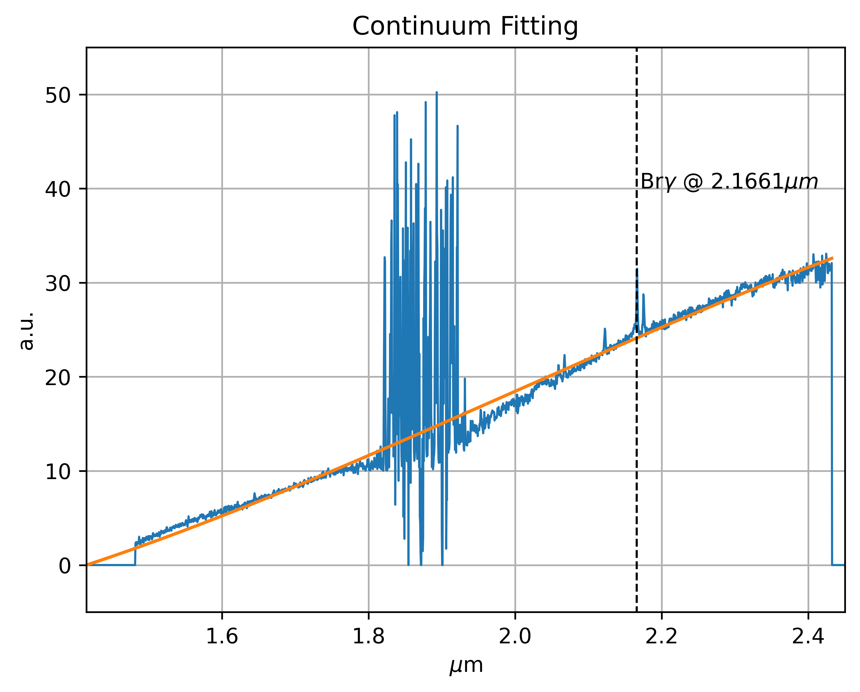
Figure 22: Example of a fit of the underlying H+K continuum of G2/DSO in 2008. We use a 2nd degree polynomial for the extracted spectrum. The Br$\gamma$ rest wavelength is marked with a dashed line. The prominent telluric absorption lines are located between $1.8\,\mu m$ and $1.95\,\mu m$. Because this spectral region is not free of confusion, we are following the argumentation of Gillessen et al. (2013a) and focus on the Br$\gamma$ analysis.

A line-map and the related channel of a data cube represents a specific wavelength and if this wavelength is Doppler-shifted, a LOS velocity $v_{z}$ with $v_{z}\,\neq\,0$ can be derived. A SINFONI 3d data cube consists of 2000+ single line maps that can also be called channels. To isolate a single line, one has to subtract the underlying continuum. Typically, a polynomial fit (here, 2nd degree) will help to get rid of the continuum and partially the background emission (see Fig. 22, Appendix B). However, the emission line itself can be heavily influenced by a variable background or atmospheric OH emission lines. For the Doppler-shifted Pa$\alpha$, HeI, and Br$\gamma$ lines that have been used for the analysis of G2/DSO (see e.g. Gillessen et al., 2013a), one has to consider the OH vibrational transition states 7-5, 8-6, and 9-7. As pointed out by Davies (2007), these OH lines do have a non-negligible influence on the shape, intensity, position, and consequently a velocity of the object of interest.

2.5 Position-Position-Velocity maps

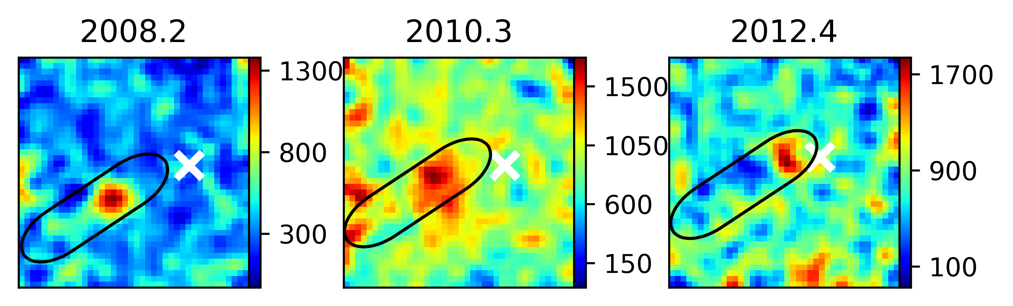
Figure 24: Smoothed PPV images. We smooth the results shown in Fig. 9 with a Gaussian smoothing kernel. Here, the surrounding noise is enhanced by the Gaussian kernel. Sgr A* is located at the position of the white $\times$. We mark the assumed position of the disputed tail emission. North is up, East is to the left. As in Fig. 9, the size of every panel is $0.5"\,\times\,0.5"$.

In this work, we study Position-Position-Velocity (PPV) maps instead of Position-Velocity (PV) diagrams because in this way we preserve more accurate information. For this purpose, we transform the Doppler-shifted wavelength information of a single pixel (i.e., spaxel) to a LOS velocity. For the analysis, we will not use a smoothing kernel since this will have an impact on the result (see Table 6 and Fig. 24, Appendix C).

2.6 Orbit analysis and MCMC simulations

Given the distance of the G2/DSO from Sgr A* and its LOS velocity evolution, we apply a Keplerian model fit to reconstruct the trajectory of the object. For the Keplerian fit, we use a SMBH mass of $M_{\rm Sgr~{}A*}\,=\,4.15\,\times\,10^{6}\,M_{\odot}$ with a distance of $d\,=\,8.3$ kpc. For the MCMC simulations, we leave the boundaries for the different parameters, except for the pericenter passage, open. Considering the uncertainty of the position of Sgr A* as well as the sensitive emission lines of the G2/DSO, we categorize different non-Keplerian interpretations of the orbit that involve more parameters (in particular the magnetohydrodynamic drag force analyzed by Gillessen et al., 2019 or the fermionic dark matter dense core-diluted halo model of Becerra-Vergara et al., 2020) as challenging and unnecessary given the current data quality.

2.7 High-pass filter

As described in Peißker et al. (2019, 2020a, 2020b, 2020d), a high-pass filter can be used to access information which is suppressed by overlapping PSF wings. Since the natural SINFONI PSF (NPSF) does show irreparable imperfections because no source is isolated in the small and crowded SINFONI FOV ($\sim\,0.8\,\times\,0.8$ arcsec), we construct an artificial PSF (APSF) with comparable parameters (x- and y-FWHM, angle with respect to North) with respect to the NPSF. For that, we fit a PSF ($\sim\,6$ pixel) sized Gaussian to S2, the brightest source in the FOV. From this, we derive the necessary input parameter to construct the NPSF. The fit uncertainties are in the range of about $1\%$.
Then, we place the input file in a $256\,\times\,256$ array. We use 10000 iterations to minimize the chance of a false positive. Furthermore, we do a background subtraction, which is of the order of $15\,-\,30\,\%$. With this procedure, the background noise can be suppressed. Subsequently, we apply the Lucy-Richardson algorithm (Lucy, 1974) and a delta map is created. By convolving this map with a suitable Gaussian kernel (around $70\%$ of the size of the input PSF), we get the final high-pass filtered image. We verify the robustness of the resulting image by comparing known stellar positions to it. In every step, the input files are normalized to the peak intensity. In most cases, the peak intensity is associated with S2. In every other case, the peak intensity is related to S35 (see Fig. 2).

2.8 OH emission lines/sky correction

The OH emission lines in the H+K band and the related correction are widely discussed by Davies (2007) and more recently by Ulmer-Moll et al. (2019). Since the emission lines of G2/DSO are Doppler-shifted, they coincide with several vibrational transitions of OH (Rousselot et al., 2000). Since Davies (2007) provides the sky correction for the SINFONI pipeline but also describes an under- and over-subtraction of various OH/sky lines in the NIR, we want to investigate the influence on the high-exposure observations carried out in the GC. The typical observation scheme for these observations is object (o) - sky (s) - object (o). However, several observational programs that are available in the ESO archive do show a nontypical observational scheme. Instead of o-s-o, these programs use o-o-s-o-o with a long exposure time of 600 seconds. This results in nonmatching sky/OH emission from the science object. Because of the exposure time, the effect is maximized.

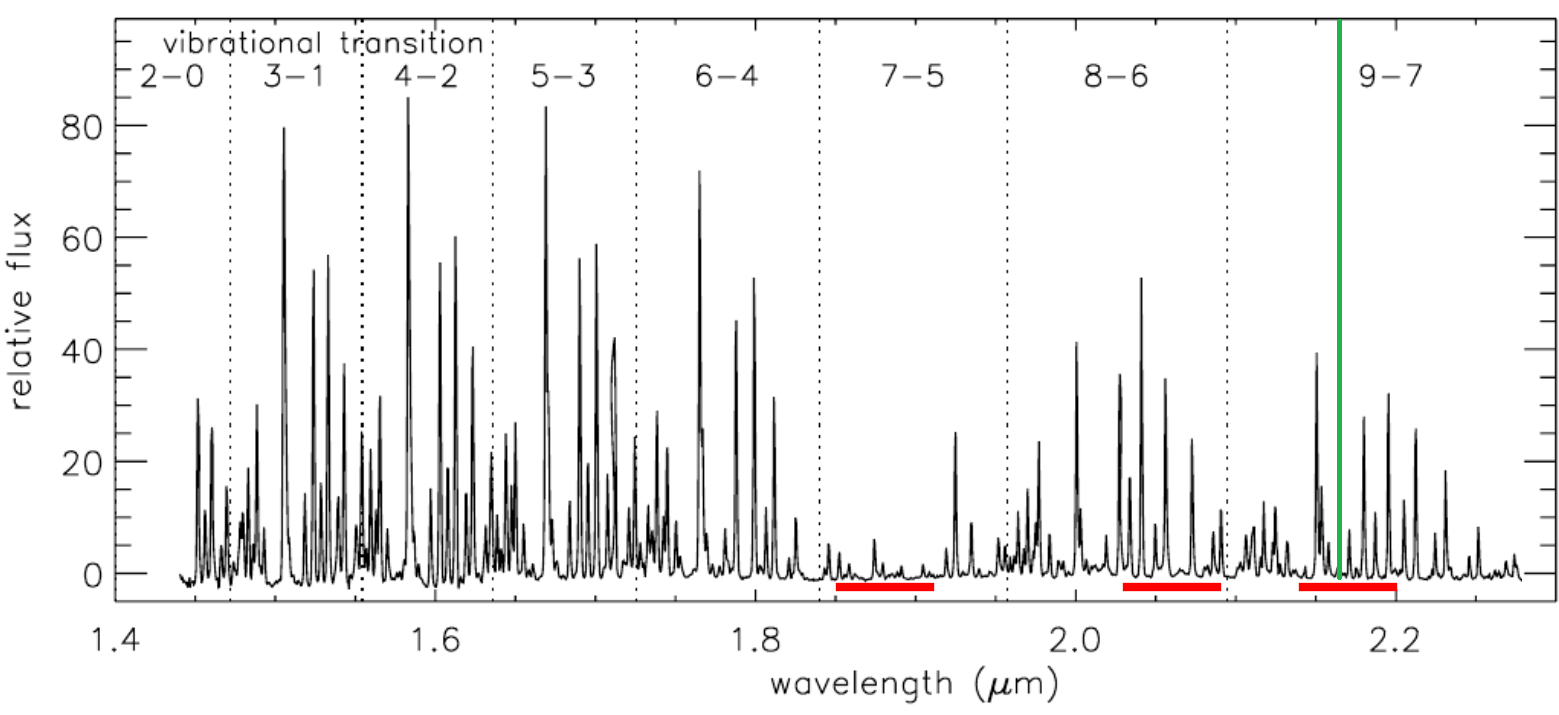
Figure 1: Near-infrared OH emission adapted from Davies (2007). We use red bars to mark the spectral range of the Doppler-shifted Pa$\alpha$, HeI, and Br$\gamma$ line that coincide with the vibrational transition states 7-5, 8-6, and 9-7 respectively. The Br$\gamma$ rest-wavelength at $2.1661\,\mu m$ is indicated with a green vertical line and embeded in the spectral region of the OH transition states 9-7 (see also Table 3).

As shown in Fig. 1, the Pa$\alpha$ line suffers from strong telluric emission/absorption features. In contrast, the OH emission lines do not influence the spectral range between $1.85-1.95\,\mu m$ at a noticeable level since the relative flux is below $10\%$. This is not valid for the Doppler-shifted HeI and Br$\gamma$ regime. Since the latter line is more prominent than the HeI line by about $40-60\%$, we will emphasize the analysis of the spectral range around the Br$\gamma$ rest wavelength of $2.1661\,\mu m$ in Sec. 3. This is consistent with the analysis and statements given by Gillessen et al. (2013a).
In Table 3, we list some prominent OH lines that could impact the line shape of the G2/DSO (see the following section).

OH line	Transition	$\lambda_{vac}$	$\lambda_{air}$
		[$\mu m$]	[$\mu m$]
Q2(0.5)	9-7	21505.044	21499.176
Q1(1.5)	9-7	21507.308	21501.440
P1(2.5)	9-7	21802.312	21796.363
P2(2.5)	9-7	21873.518	21867.550

Table 3: OH lines as observed in the NIR at Paranal by Rousselot et al. (2000). Because of the Doppler-shift of the Br$\gamma$ line of the G2/DSO, these OH lines interfere with the observed source emission.

3 Results

In this section, we present the main results of the observational analysis. First, we will present line maps that show the G2/DSO approaching Sgr A*. For comparison, the data between 2014.5-2019.5 cover the approaching post-pericenter part of the G2/DSO orbit, which will be shown afterwards. Markov-Chain-Monte-Carlo (MCMC) simulation emphasizes the robustness of the orbital elements. Non-smoothed PPV maps investigate a possible velocity gradient of the G2/DSO. The $K$-band detection of the G2/DSO emphasizes the stellar nature of the object. This is followed by the analysis of the proposed tail (Sec. 1) and the identification of the additional sources OS1 and OS2.

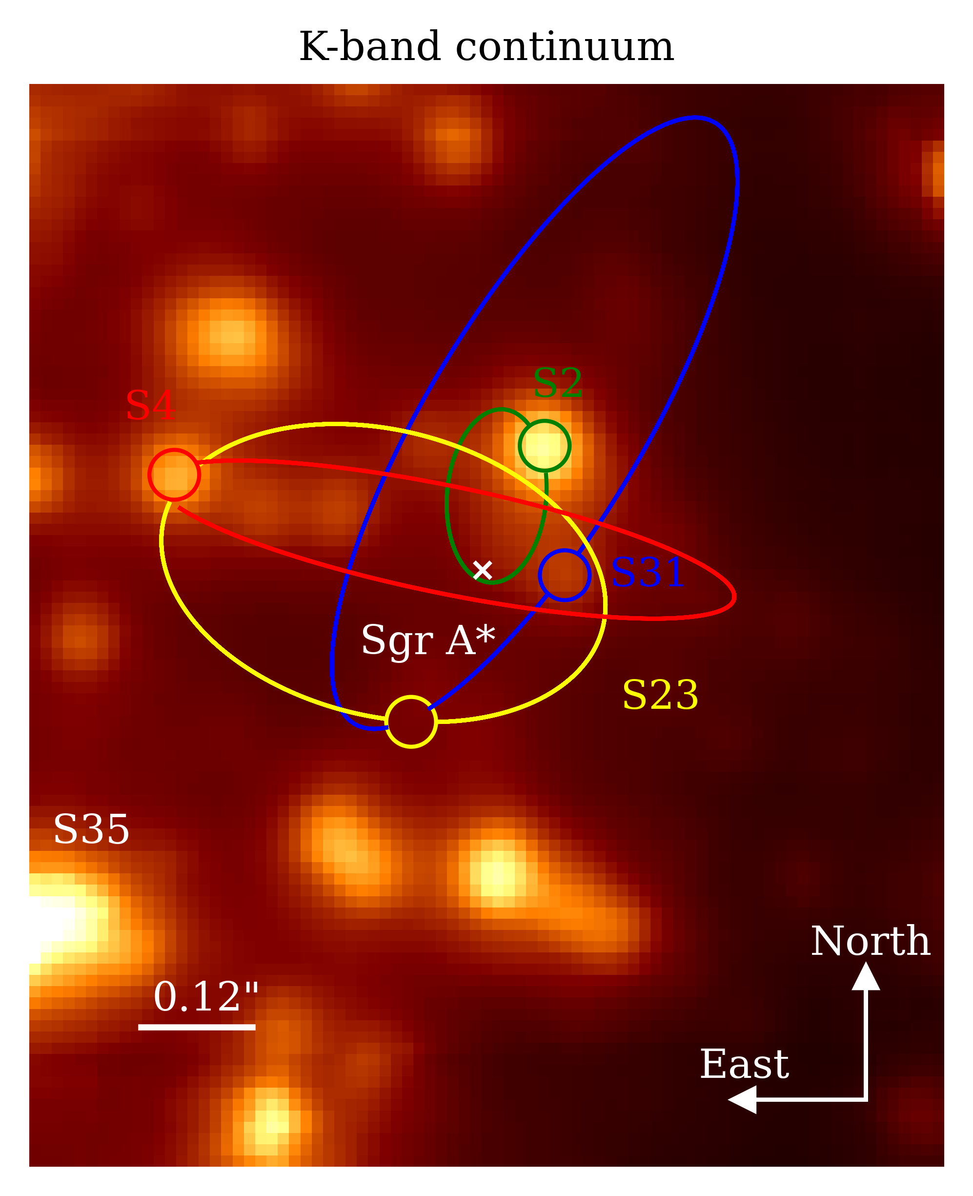
Figure 2: Finding chart of the S-cluster. The x marks the position of Sgr A*, the green line represents the Keplerian orbit fit of S2. In addition we show the orbits of S4, S23, S31, and S35. The image is extracted from a SINFONI data cube by collapsing the wavelength range between $2.0\,\mu m\,-\,2.2\,\mu m$ (K-band). The observation took place in 2014 and the total on-source integration time is 24 hours (216 single cubes, 400 seconds each).

To provide a confusion-free overview of the S-cluster, please see the finding chart in Fig. 2 where we mark the most prominent $K$-band source S2, the related orbit, and the in this work discussed stars.

3.1 Line map detection

The line maps (Fig. 3) are extracted from the final mosaic data cube of the related year. We emphasize the investigation of the red-shifted (until 2014.3) and blue-shifted (after 2014.4) Br$\gamma$ line. After the Doppler-shifted Br$\gamma$ line is selected, we subtract the underlying continuum. In every dataset, the G2/DSO can be identified without confusion. The local background, the distance to the surrounding stars, weather conditions, and the on-source integration time do have a major impact on the shape of the source (see Fig. 3). The line maps show the obvious periapse of the G2/DSO in 2014. Since the source can exclusively be observed in the redshifted Br$\gamma$ regime until 2014.35 and subsequently in the blueshifted domain after 2014.45, the periapse passage must have happened in between.

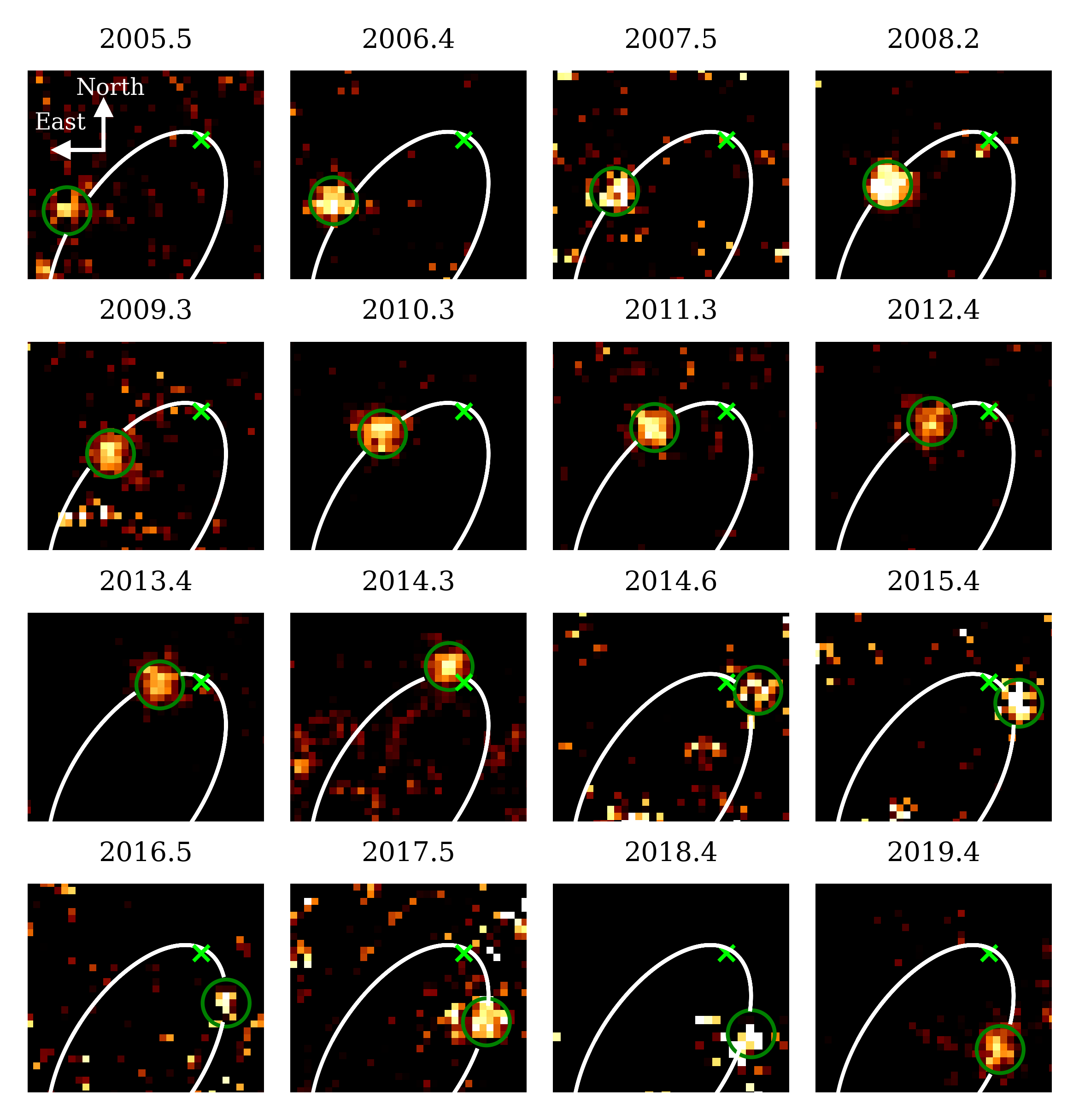
Figure 3: Doppler-shifted Br$\gamma$ line evolution of the G2/DSO as it approaches and passes around Sgr A*. The $\times$ marks the position of Sgr A*, the green circle indicates the position of the G2/DSO. North is up, east is to the left. As discussed in Valencia-S. et al. (2015), the forth-shortening factor converges to unity around 2014.3 where we are able to observe the true size of the G2/DSO at the periapse. The orbital trajectory (in white) is adapted from the fit presented in Sec. 3.2.

In the following, we use the identification of the G2/DSO in the line maps to derive an exact value for the time of periapse from the Keplerian model fit.

3.1.1 Br$\gamma$ line evolution for G2/DSO, OS1, and OS2

Based on the clear line map detection of the G2/DSO between 2005 and 2019, we extract the source spectrum to derive several properties (Fig. 4). To that goal, we use an aperture with a radius of 2 pixel (25 mas). We subtract an aperture with an inner radius of 3 pixel and an outer radius of 10 pixels because of the dominant background/continuum. Then, we fit a polynomial function to the spectrum and fit a Gaussian to the Br$\gamma$ line (see Table 4). With this procedure, we derive the LOS velocity for the G2/DSO as well as the line width $\sigma$. By studying $\sigma$ as a function of time, we find a quadratic behavior of the Br$\gamma$ line width (Fig. 5 and Fig. 25, Appendix D). We note that the gradient is expected to be the largest around the time of periapse because of the viewing angle change and the foreshortening factor close to unity (see the following subsection).

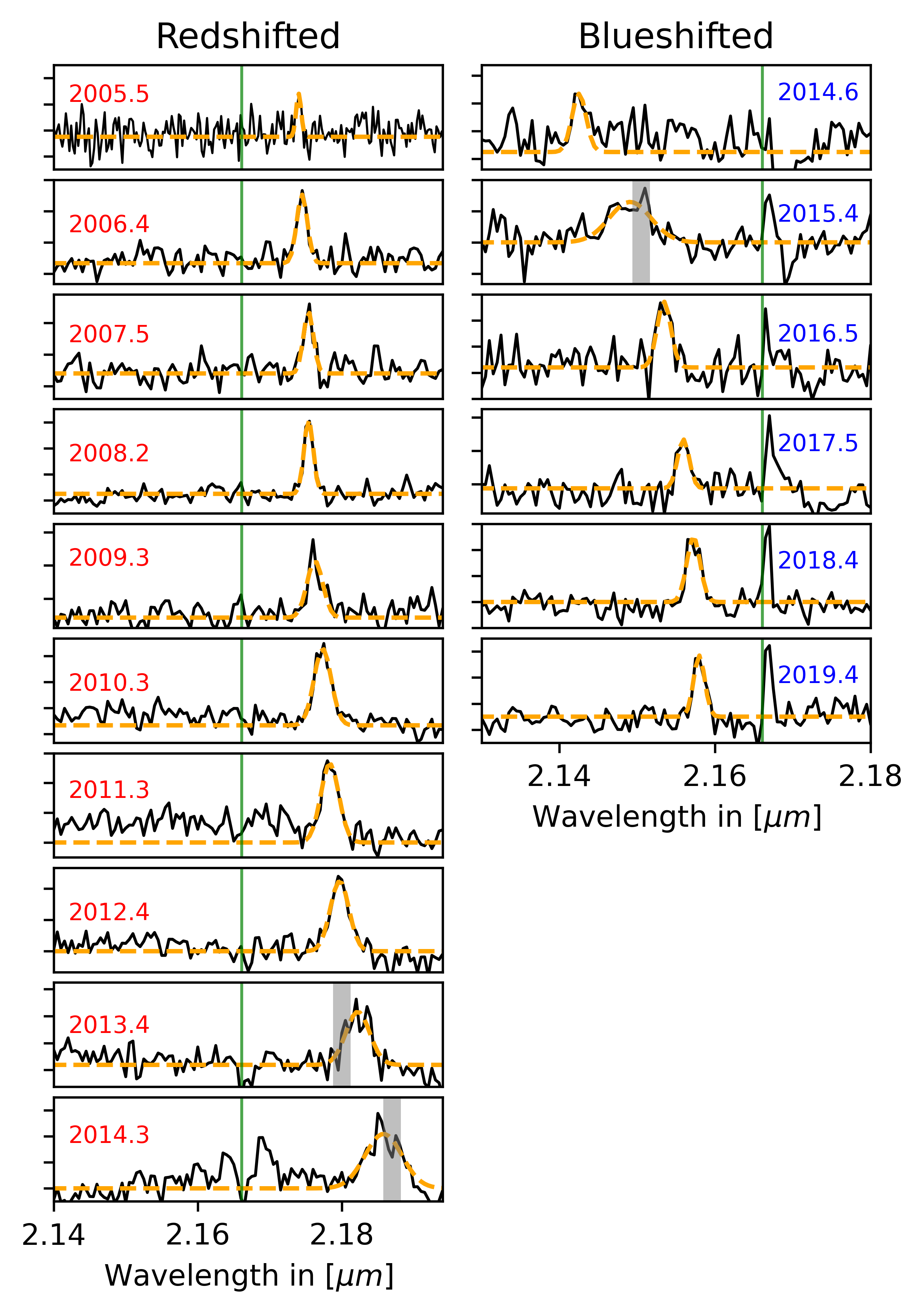
Figure 4: Doppler-shifted Br$\gamma$ line evolution between 2005 and 2019. The green line marks the Br$\gamma$ rest wavelength at $2.1661\mu m$. The grey bars indicate the spectral position of the OH lines Q1, Q2, P1, and P2 (see Sec. 2.8 and Table 3) that blend with the Dopper-shifted Br$\gamma$ line.

Throughout the years, the PSF size of the source is $\sim 75\,-\,100$ mas in x- and y-direction, therefore the G2/DSO can be described as compact (Table 4).

Epoch	Wavelength in [$\mu m$]	Velocity in [km/s]	Standard deviation $\sigma$ in [km/s]	Line map size in [mas]
				x (R.A)	y (DEC.)
2005.5	2.1740	1094.69	48.97	65	40
2006.4	2.1744	1159.96	102.51	94	78
2007.5	2.1753	1282.89	96.60	71	60
2008.2	2.1753	1287.36	87.06	74	73
2009.3	2.1762	1405.98	151.64	68	69
2010.3	2.1773	1555.53	165.31	89	74
2011.3	2.1783	1693.99	174.92	85	94
2012.4	2.1796	1881.95	180.40	71	76
2013.4	2.1822	2231.68	229.72	90	98
2014.3	2.1857	2726.20	355.02 (234.31)	51	59
2014.6	2.1425	-3265.23	126.74	56	74
2015.4	2.1490	-2355.72	369.12 (243.61)	60	86
2016.5	2.1534	-1752.34	122.32	31	55
2017.5	2.1559	-1407.56	104.67	69	86
2018.4	2.1572	-1228.13	119.71	56	64
2019.4	2.1579	-1126.27	98.87	61	85

Table 4: Spectral and line map properties of the G2/DSO. Please see Fig. 4 for the related fit. Here, the standard deviation $\sigma$ is a measure of the line width. The size is measured by using a 6 pixel Gaussian fit. Usual uncertainties for the size of the G2/DSO are in the range of 12.5 mas. For the values in 2014.3 and 2015.4, please see Sec. 2.8 and Sec. 4. Here, the format of the time is given in decimal years.

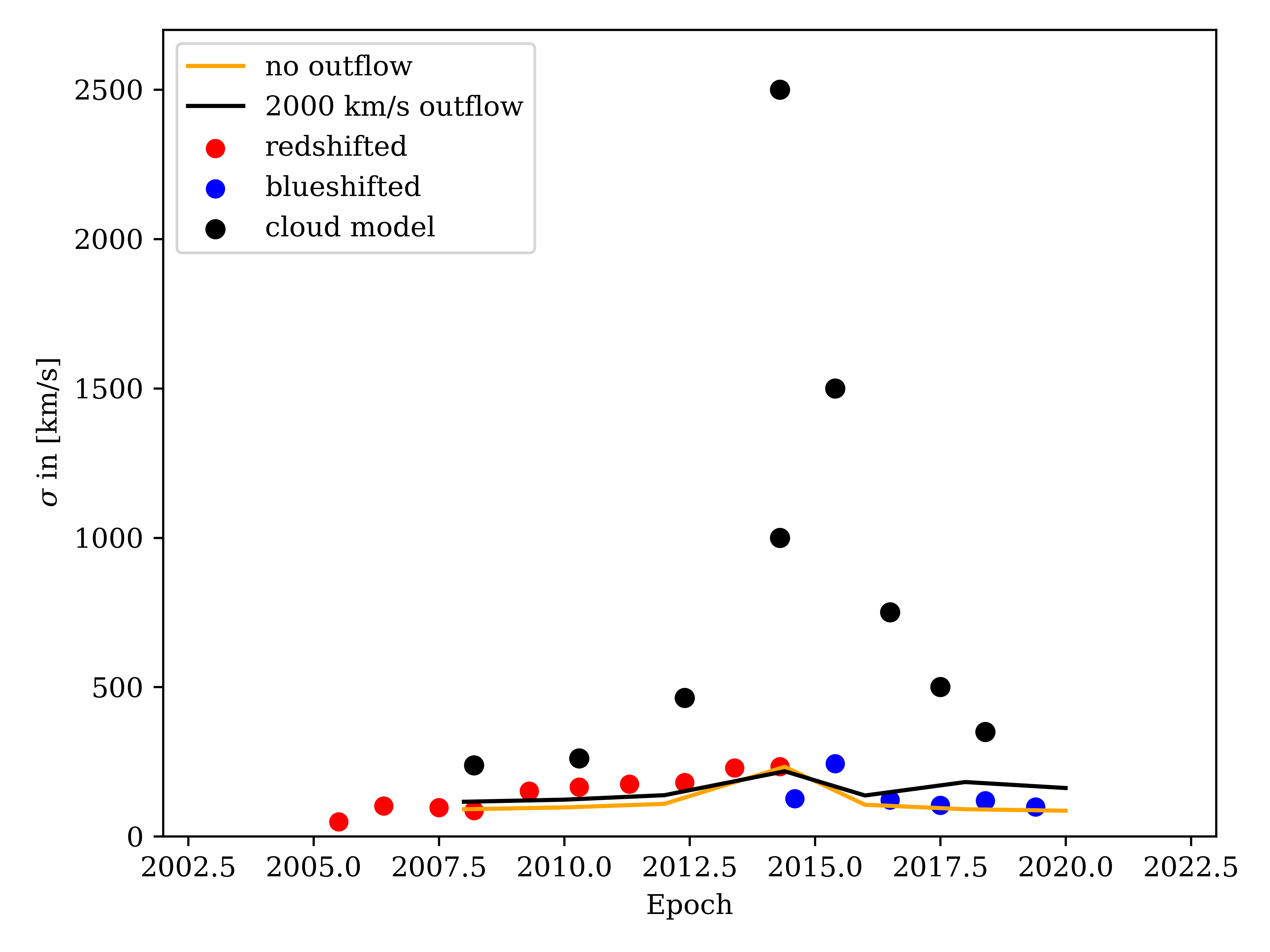
Figure 5: Standard deviation as a measure of the line width $\sigma$ of the Br$\gamma$ line expressed as a function of time. Black data points are based on the cloud model (see, e.g., Gillessen et al., 2019). Red datapoints describe the pre-periapse measurements, while blue datapoints represents the measurements in the post-periapse phase. Orange and black lines are referring to the model calculations of line widths corresponding to the bow-shock velocity field without and with a nuclear outflow, respectively, see Zajaček et al. (2016). Typical uncertainties for the line width are here $\pm\,30$ km/s. Especially the data points in 2014.3 and 2015.4 suffer from the inefficient OH line correction (vibrational transition 9-7) as shown in Fig. 1 (see Sec. 2.8) and Table 3. At $2.1505\,\mu m$, $2.1507\,\mu m$, and $2.1873\,\mu m$ the OH lines are infecting the line width of the Br$\gamma$ emission of the G2/DSO. Hence, the data points of 2014.3 and 2015.4 are corrected values (see Sec. 4.7). For a complete overview of the K-band OH lines and the corresponding relative intensities, see Rousselot et al. (2000). See Fig. 25, Appendix D for a zoomed in view of the same figure.

The related spectral line fits and tables for OS1 and OS2 can be found in the Appendix E (see Fig. 26, Fig. 27, and Table 14).

3.2 Orbit

As mentioned in Sec. 2 and shown in Fig. 2, we use the orbit of S2 to derive the position of Sgr A* with a positional uncertainty of 12.5 mas (= 1 pixel). We list the orbital elements that are adapted from Peißker et al. (2020a) in Table 5. For the Keplerian orbital fit, we extract the G2/DSO position with a Gaussian fit that simultaneously provides a positional uncertainty. Since this value would underestimate the unstable character of the data, we adapt the common uncertainty of 12.5 mas for the spatial position of the G2/DSO with respect to Sgr A*. Please consider Table 15, Appendix F for the derived relative position with respect to Sgr A*. The related LOS velocities can be found in Table 4.
In Figure 6, we show the outcome of the Keplerian model fit. This solution underlines the Keplerian trajectory of the G2/DSO. The best-fit orbital elements are listed in Table 5.

Figure 6: A Keplerian orbit of the G2/DSO based on the Doppler-shifted Br$\gamma$ emission line. The upper panel shows the on-sky projection of the source. The middle and lower panels show the spatial RA and DEC position as a function of time, respectively. The closest approach to the SMBH can be observed in 2014.38. Given the uncertainties, we find a good agreement of the G2/DSO trajectory with a Keplerian model fit.

Based on the orbital elements, we find that a periapse passage of the G2/DSO occurred in $\sim 2014.38$, which is in agreement with the line map detection (see the following subsection and Fig. 3) as well as with the earlier calculation of the pericenter passage presented in Valencia-S. et al. (2015), where the authors report $t_{\rm closest}=2014.39\pm 0.14$.

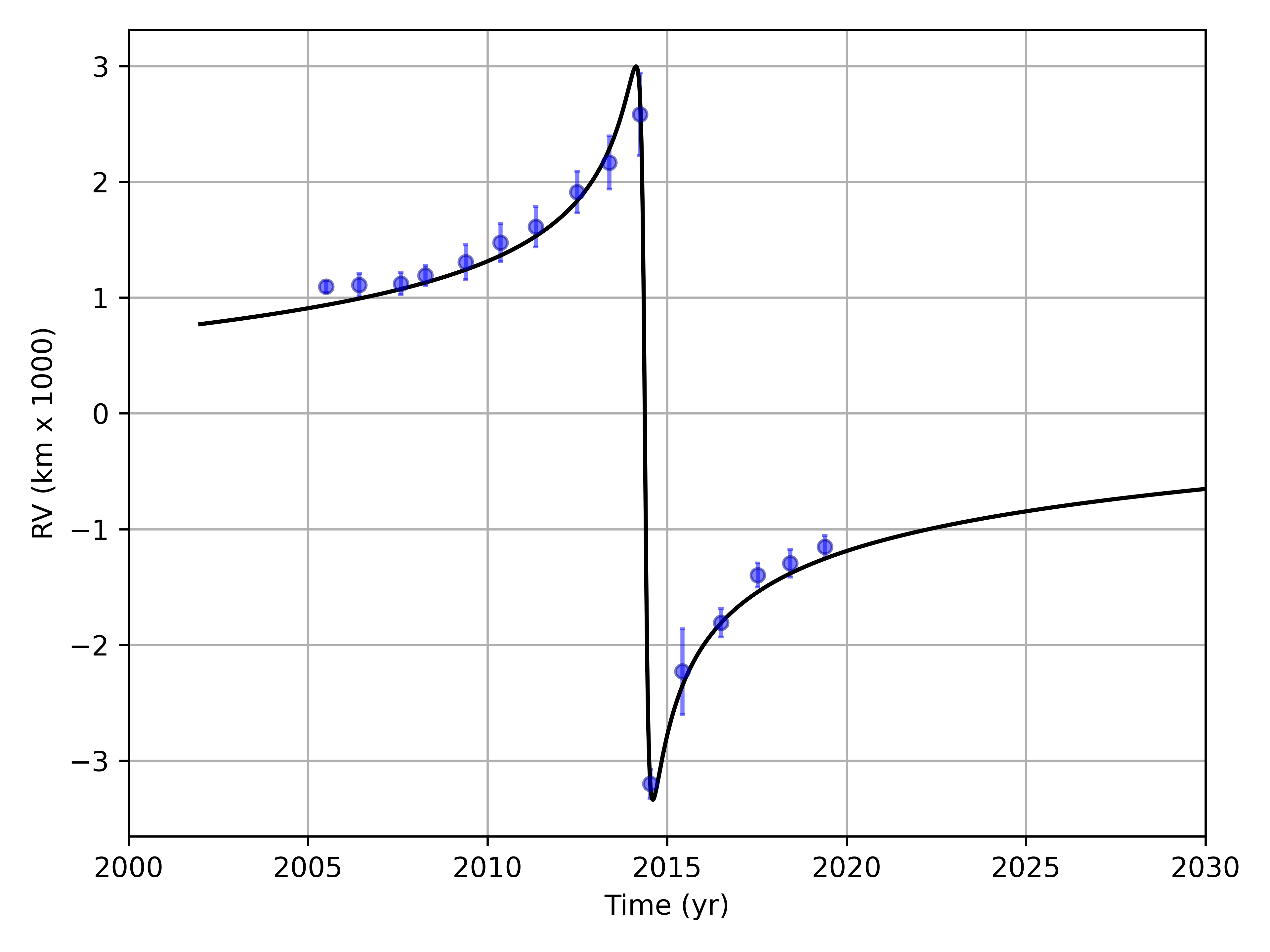
Figure 7: Line-of-sight velocity $v_{z}$ of the G2/DSO as a function of time. As displayed, the G2/DSO accelerates until 2014.3 in the redshifted Br$\gamma$ domain. After 2014.38, the velocity is blueshifted as the G2/DSO continues its way on a Keplerian orbit. The uncertainties are adapted from Table 4.

In Fig. 7, we furthermore show the LOS velocity evolution of the G2/DSO as a function of time. The absolute value of the LOS velocity of the G2/DSO reaches $3338\,{\rm km/s}$. The common uncertainty for the velocities is $\pm\,35\,{\rm km/s}$ (see Peißker et al., 2020b). We use the orbital elements given in Table 5 to investigate the statistical robustness (Fig. 29, Appendix G). The MCMC simulations agree with the initial input parameters. Since the uncertainty does not reflect the character of the data nor the observations, again we choose a more conservative approach and round up the range of possible values.

Source	$a$ (mpc)	$e$	$i$(o)	$\omega$(o)	$\Omega$(o)	$t_{\rm closest}$(yr)
S2	5.04 $\pm$ 0.01	0.884 $\pm$ 0.002	136.88 $\pm$  0.40	71.33 $\pm$ 0.75	234.51 $\pm$ 1.03	2002.32 $\pm$ 0.02
G2/DSO	17.45 $\pm$ 0.20	0.962 $\pm$ 0.004	58.72 $\pm$ 2.40	92.81 $\pm$ 1.60	295.64 $\pm$ 1.37	2014.38 $\pm$ 0.01

Table 5: Orbital elements of S2 and G2/DSO as shown in Fig. 2, 3, 6. The orbital parameters for S2 are adapted from Peißker et al. (2020a) and are used to determine the position of Sgr A*. As estimated in the text, the closest pericentre approach of G2/DSO is about $0.66\,{\rm mpc}$ or $16.5\,{\rm mas}$ / $137\,{\rm AU}$.

The final uncertainties for the orbital elements (which are based on the Keplerian fit) are given in Table 5. Additional results of this analysis are the mass $M_{\rm Sgr~{}A*}$ of Sgr A* of about $M_{\rm Sgr~{}A*}\,=\,4.15\,\times\,10^{6}\,M_{\odot}$ and the distance $d$ to the GC of $d\,=\,8.3$ kpc. Based on the orbital elements, we find a pericentre distance $r_{\rm p}$ of $r_{\rm p}\,=\,a(1-e)\,\approx\,0.66\,{\rm mpc}$.

3.3 Periapse of the G2/DSO in 2014.38

Since the literature suffers from inconsistencies regarding the nature of the G2/DSO or the general periapse sequence (Gillessen et al., 2012; Witzel et al., 2014; Valencia-S. et al., 2015; Pfuhl et al., 2015), we focus on the observations that cover the epoch of 2014. Since it was predicted and shown that the gas cloud G2/DSO can be observed simultaneously before and after its periapse, we will investigate the region of interest (see Fig. 4 shown in Gillessen et al., 2019). In combination with the velocity (and hence wavelength) information given in Pfuhl et al. (2015), we show in Fig. 8 the reported area of the blueshifted part of G2/DSO in 2014.3 (216 single exposures), 2014.6 (94 single exposures), and 2014.5 (310 single exposures).

Figure 8: Line maps that cover a range of about $1500\,{\rm km/s}$. This range is based on the PV diagrams as presented in Pfuhl et al. (2015). The white arrow marks the expected position of the blueshifted component of the G2/DSO based on the analysis presented in Plewa et al. (2017) and Gillessen et al. (2019). We mark the derived Keplerian position of the G2/DSO with a green circle (see Fig. 3). The noisy character of the SINFONI line maps is here indicated by the intensity variation of the pixels. Because of the wide velocity range that is representative for the spectral range $2.145\,\mu m\,-\,2.155\,\mu m$ (120 channels), the line map is noise dominated which hinders the detection of the G2/DSO. For each line map, we subtract the averaged 10 neighboring channels of the spectral range. Sgr A* is located at the white $\times$. The size of every panel is $0.42"\,\times\,0.37"$.

Based on the information of the published data (see Fig. 15 in Pfuhl et al., 2015), we select the wavelength range $2.145\,\mu m\,-\,2.155\,\mu m$ which corresponds to the blueshifted velocities $1537\,-\,2922\,{\rm km/s}$. As shown in Fig. 8, the line maps suffer from noise and artefacts. This is consistent with Valencia-S. et al. (2015) where the authors encounter the same situation. However, we do not agree with the smoothed and artificially enhanced emission (the authors call it ‘scaling adjustment’) that is shown in Pfuhl et al. (2015) for 2014.3. The G2/DSO in Fig. 8 cannot be observed since the line maps are noise dominated (that is due to the large selected spectral range). We advise the interested reader to compare the significance of the Br$\gamma$ emission in Fig. 3 with Fig. 8. We will discuss this result in detail in Sec. 4.

3.4 Position-Position-Velocity maps

According to Pfuhl et al. (2015), a clear velocity gradient should be observable, especially in the pre-pericentre phase of the G2/DSO. To maintain the overall shape of the data and hence provide a certain level of comparability with the pipeline results (i.e., the output mosaic data cube), we use PPV diagrams. We favor this approach since the spatial dimensions of a PV diagram are reduced to one parameter which can result in confused detections. Since the outcome of a PV diagram purely rely on the derived orbit, we question the capability of this technique in the first place. However, for the here presented PPV plots, the spectral pixel information is transformed to a velocity. In Fig. 9, we present a selected overview of the pre-periapse time of the G2/DSO. We divide the investigated spectral range of each year into equal-sized sections (i.e., spectral slices) and we subtract the neighboring channels. Following this procedure, we preserve the information and avoid a disintegration of the emission.
By comparing the PPV plots, no prominent velocity gradient is present. Furthermore, the data again suffer from artefacts and noise. We underline that we do not use any Gaussian smoothing kernel to enhance nonlinear parts of the G2/DSO.

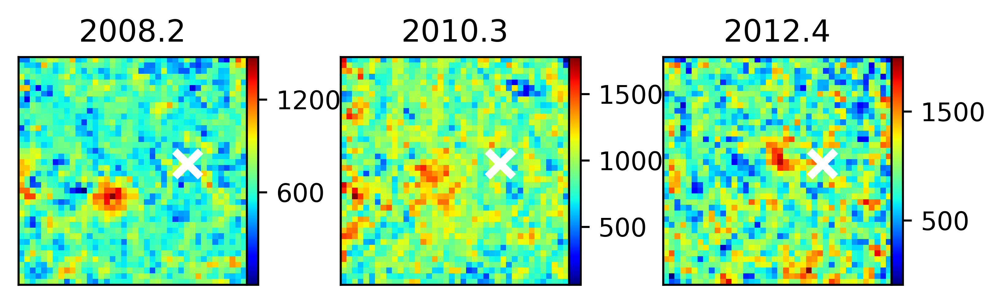
Figure 9: Position-Position-Velocity maps of the G2/DSO for 2008, 2010, and 2012 epochs. North is up, East is to the left. The size of every panel is $0.5"\,\times\,0.5"$. The position of Sgr A* is indicated with a white $\times$. We pick these epochs since the velocity gradient as claimed by Pfuhl et al. (2015), Plewa et al. (2017), and Gillessen et al. (2019) should be traceable with reduced confusion compared to other years. In Fig. 24, we present a smoothed version of this figure. A detailed discussion of the result is given in Sec. 4.

Since the background subtraction influences the shape of the Doppler-shifted Br$\gamma$ emission line (see Appendix C), the velocity distribution may contain artefacts. Please see a smoothed version of Fig. 9 and a possible tail emission in Appendix C, Fig. 24. In the following, we will investigate the influence of the sky emission on the data.

3.4.1 Artificial velocity gradient

As previously discussed in Sec. 2, we analyse the efficiency of the sky correction in case the object- and sky-observations contain irregularities. For that purpose, we manipulate the sky correction with an error of $-10\%$ of the maximum flux of the input files , i.e., we subtract $10\%$ of the peak emission of the sky frames. Furthermore, we smooth the original position-position-velocity map with a one pixel Gaussian. The results of this analysis are listed in Table 6.

	2008	2010	2012
	$\left[{\rm km/s}\right]$	$\left[{\rm km/s}\right]$	$\left[{\rm km/s}\right]$
Expected gradient	$\pm 45.58$	$\pm 78.77$	$\pm 101.2$
No error	$\pm 19.97$	$\pm 37.01$	$\pm 63.77$
$10\%$ error	$\pm 35.99$	$\pm 88.27$	$\pm 138.58$
Smoothed, 1 px	$\pm 80.46$	$\pm 143.94$	$\pm 200.5$
Plewa et al. (2017)	$\pm 238$	$\pm 261$	$\pm 464$

Table 6: Influence of a poor sky correction and Gaussian smoothing on the velocity gradient. Details are given in the text.

While combining the observational data of an object for each year leads to a natural velocity gradient because of the intrinsic motion (“expected gradient"), we find lower values for the Br$\gamma$ emission of the G2/DSO. Since the observations do not cover a complete year, this result is expected. However, measuring the velocity gradient of the G2/DSO in the sky manipulated data shows increased values that are close or over the expected values. Smoothing the data increases the velocity gradient by about $30-50\%$. As shown in Fig. 9, the noisy character of the data is responsible for this increased velocity gradient. Hence, smoothing data impacts the outcome of the velocity gradient analysis.

3.5 K-band detection

To investigate the possibility of a stellar source that is associated with the observed Doppler-shifted Br$\gamma$ line emission, we apply the Lucy-Richardson algorithm to the data (see also Peißker et al., 2020b). We select the $K$-band in the related data cube and apply a background emission of $15-30\%$ of the peak intensity emission depending on the variable background. With this approach, we eliminate the chance of a false positive.

Figure 10: High-pass filtered $K$-band images of the GC region with the focus on the Keplerian G2/DSO orbit. The location of Sgr A* is indicated with a lime colored $\times$. The size of each panel is $0.4"\,\times\,0.3"$. North is up, East to the left. The green contour lines are at $10\%,\,30\%,\,50\%,\,70\%,$ and $90\%$ of the normalised S2 peak intensity. The lightblue colored contour lines are adapted from the Doppler-shifted Br$\gamma$ emission shown in Fig. 3. Because of the high stellar density, the position of the K-band counterpart of G2/DSO may be confused. We refer the reader to the Appendix F, Fig. 28, where we show the extracted K-band continuum position of G2/DSO and compare it to the here derived orbit.

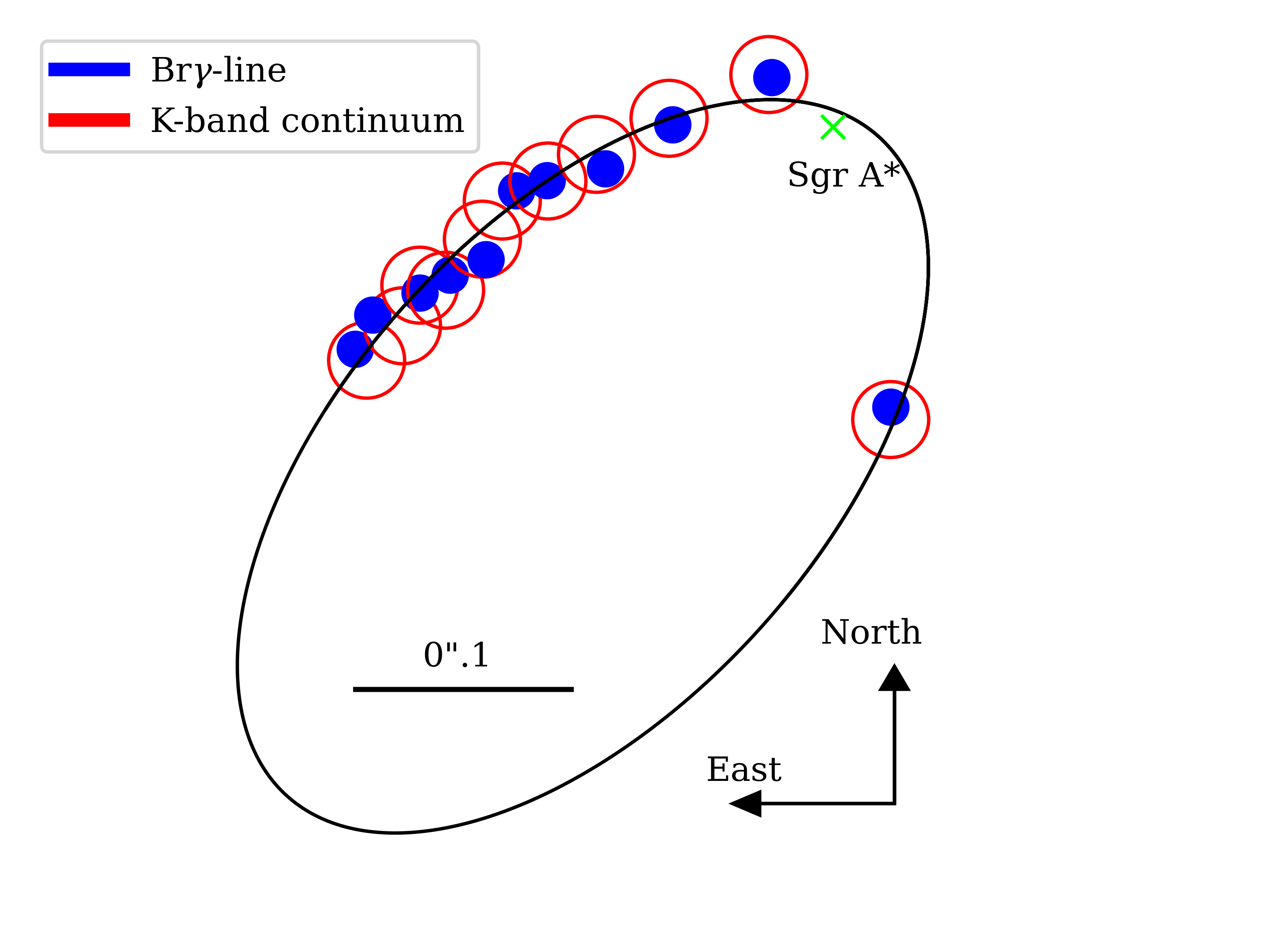
Figure 28: K-band continuum positions (red circle) derived from the high-pass filtered detection of G2/DSO as presented in Fig. 10. From Fig. 3, we include the Br$\gamma$ line detection (blue points) for comparison. The lime colored $\times$ marks the position of Sgr A*. In 2015–2017 and 2019, the K-band counterpart of G2/DSO is confused with S23 and S31.

In Fig. 10, we present the resulting convolved images. In agreement with the position of the Doppler-shifted Br$\gamma$ line emission, we detect a source that is approaching and passing Sgr A* on a trajectory comparable to the G2/DSO. By comparing the K-band continuum position with the Br$\gamma$ detection shown in Fig. 3, we find a small offset of $\leq\,12.5$ mas ($\sim 100$ AU) between the centroid of the stellar source and the line emission. For this comparison, please consider Fig. 28, Appendix F. In 2016 and 2017, S31 and S23 (see Fig. 2) coincide with the blueshifted G2/DSO Br$\gamma$ line position.

3.6 Stellar K-band magnitude

To investigate the $K$-band continuum magnitude and the flux density evolution of the G2/DSO along the orbit, we use the detection of the high-pass filter analysis shown in Fig. 10. For the analysis, the zero magnitude flux is set to $653$ Jy and an effective wavelength of $2.180\,\mu m$ is applied. These settings are related to the ESO $K$-band filter (for comparable values, see also Tokunaga & Vacca, 2007).

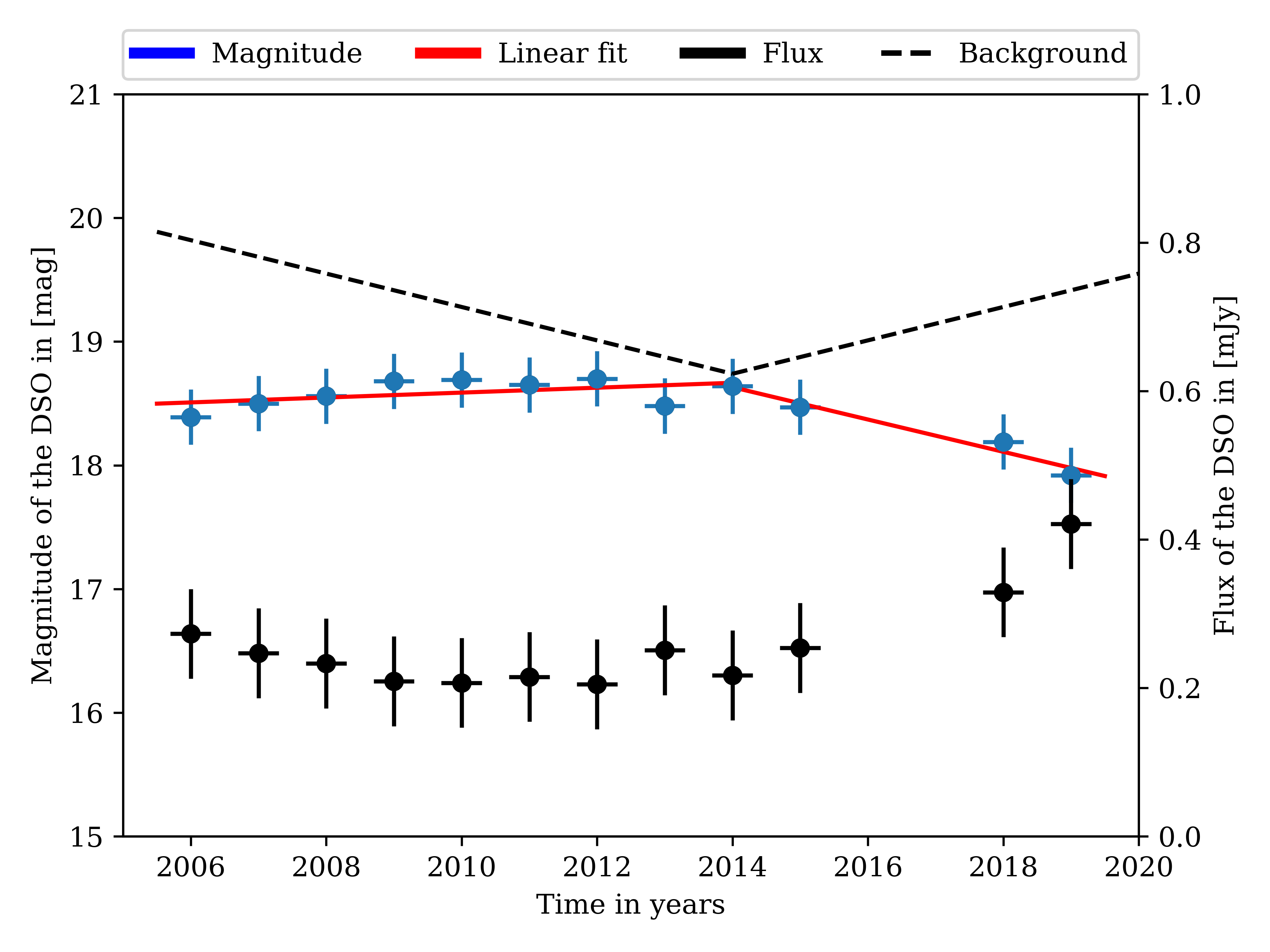
Figure 11: $K$-band flux and magnitude of the G2/DSO based on the high-pass filter detection. The blue data points are related to the magnitude where lower values correspond to a brighter emission. Black data points represent the magnitude-correlated flux. The error bars represent the standard deviation. The dashed black line corresponds to the observed background magnitude which is measured at a distance of $\sim\,40$ mas to G2/DSO. In 2014, G2/DSO reaches pericenter. Hence, this epoch represents the closest distance towards Sgr A* which correlates to the increased background light. The derived slope of $0.13$ of the observed background magnitude agrees with the analysis presented in Sabha et al. (2012).

For the magnitude, we use the extinction-corrected S2 magnitude of 14.15 mag. In the following, we adopt the bolometric magnitude relation with

$$m_{\rm{G2/DSO}}\,=\,-14.15\,+\,2.5\,\times\,\log(\mathrm{ratio})$$ (1)

where ‘ratio’ is defined as the counts of the object of interest (here G2/DSO) and the reference star. Since we normalize the data to the flux of S2, ‘ratio’ simplifies to the counts of the G2/DSO. Because of confusion, we exclude the data points of 2005, 2016, and 2017. While the uncertainty is based on the standard deviation, we find an average magnitude of the G2/DSO of $18.48\,\pm\,0.22$ mag. For the averaged flux $f$, we adapt

$$f_{\rm G2/DSO}\,=\,f_{\rm S2}\,\times\,10^{-0.4(\mathrm{mag}_{\rm G2/DSO}-\mathrm{mag}_{\rm S2})}$$ (2)

from Sabha et al. (2012) to calculate the related flux density of G2/DSO with $f_{\rm S2}\,=\,14.23\,$mJy and $\mathrm{mag}_{\rm S2}\,=\,14.1$. We get $0.25\,\pm\,0.06\,$mJy which is fully consistent with the literature.
Comparing the pre- and post-periapse epochs, we find a slightly decreasing magnitude towards Sgr A*. This is expected since Sabha et al. (2012) shows that the density of (old) faint stars increases towards Sgr A*. To eliminate the chance that the here presented magnitude is correlated to background fluctuations or nearby stars, we measure its intensity close to G2/DSO with a one-pixel aperture at a distance ($\sim\,40$ mas) larger than the radius of the SINFONI PSF ($31.25-37.5$ mas). Based on Fig. 11, we find that neither the pre- nor post-periapse data is correlated to background fluctuations or surrounding stars. It is reasonable to assume, that the K-band magnitude of G2/DSO would increase because of close-by stars or the dominant background light towards Sgr A*. In Section 4, we will elaborate on the here mentioned points.

3.7 The “tail"

As it is already shown and described in Peißker (2018), we created a series of PV diagrams inspired by Gillessen et al. (2012) where the authors show the gas cloud G2/DSO and its tail component with a Keplerian orbit approaching Sgr A*. Since Gillessen et al. (2012) smooth parts of the presented image (see the dotted box in the left panel of Fig. 12), we investigate the non-smoothed emission between $2.1661\,\mu m$ and $2.182\,\mu m$ in contrast.

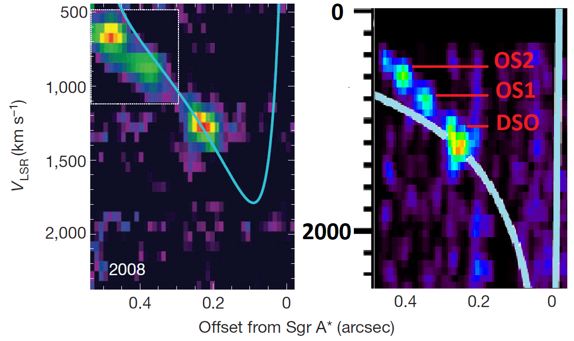
Figure 12: Comparison of Position-Velocity diagrams of 2008 adapted from Gillessen et al. (2012) (left panel) and Peißker (2018) (right panel). The dotted box in the left panel shows smoothed emission. The emission outside the dotted box is not smoothed. The right panel is not treated with an dominant Gaussian kernel and reveals the two isolated sources OS1 and OS2 that are temporarily close to G2/DSO. In both panels, the Keplerian orbit is shown in lightblue.

Without an imperious smoothing kernel that is applied to the data, we confirm emission at the position of the so-called tail that is above the noise level. However, we cannot agree with the interpretation of this emission since we detect isolated sources that show temporary close distance to the G2/DSO (see the right panel of Fig. 12). In the following subsections, we will investigate these sources, which we refer to as OS1 and OS2, in detail. Additional material covering the so-called tail can be found in the Appendix C, see Fig. 23 and Fig. 24.

3.7.1 OS1

As indicated in Fig. 12 (right panel), we identify OS1 in several epochs following the G2/DSO on a similar orbit (see Fig. 13 and Fig. 17). In several epochs, the identification of OS1 suffers from a decreased data quality and nearby stellar sources.

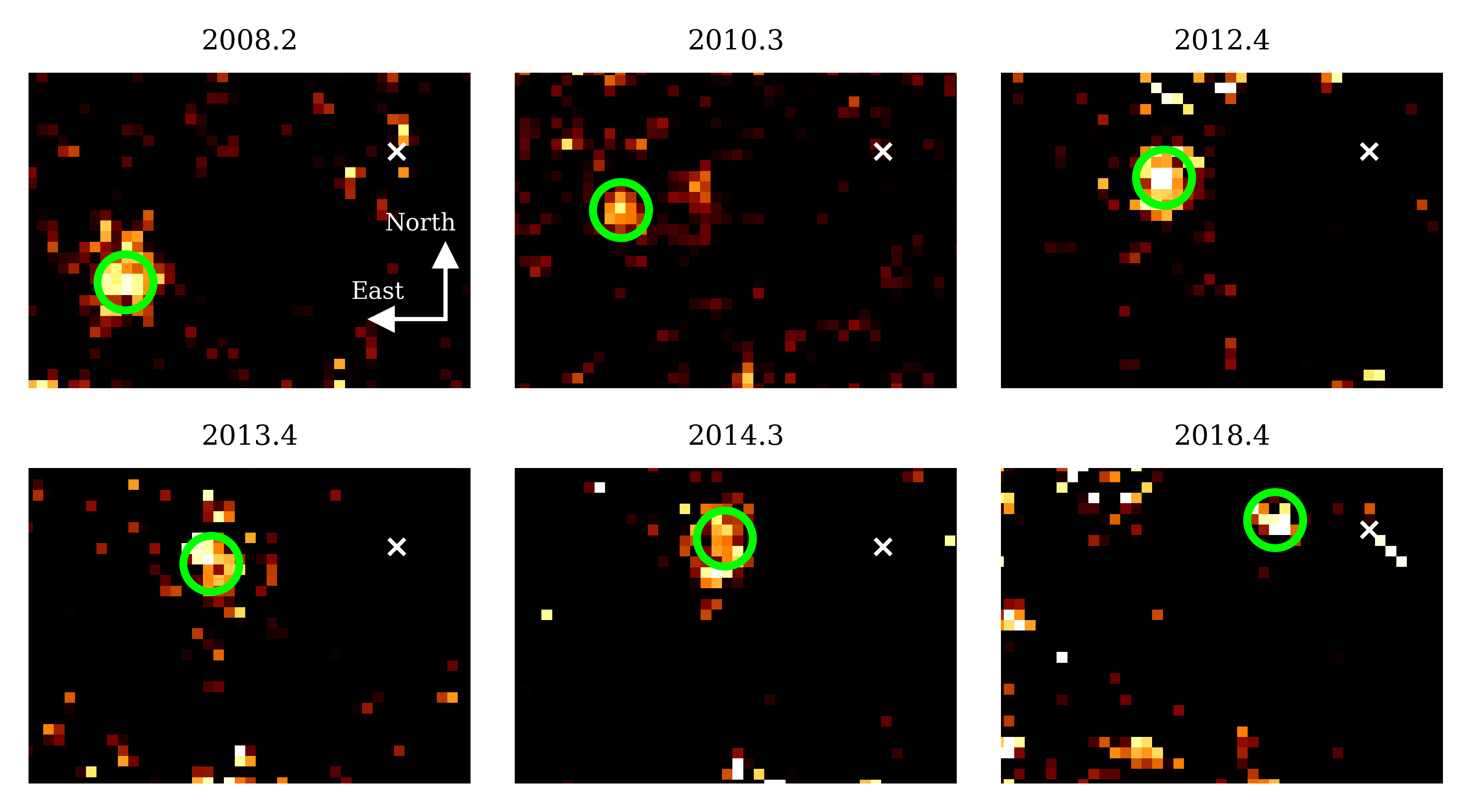
Figure 13: The detection of OS1 in the Doppler-shifted Br$\gamma$ regime (marked with a lime-colored circle). As indicated, North is up, East is to the left. The position of Sgr A* is marked with a white $\times$.we note that OS1 is consistent with compact object seen at the diffraction limit of the telescope. The size of each panel is $0.52"\,\times\,0.37"$.

Using the extracted positions, we derive an orbit for OS1 (see Fig. 14). The uncertainties reflect the distance to nearby stellar sources and include the discussed Sgr A* position range.

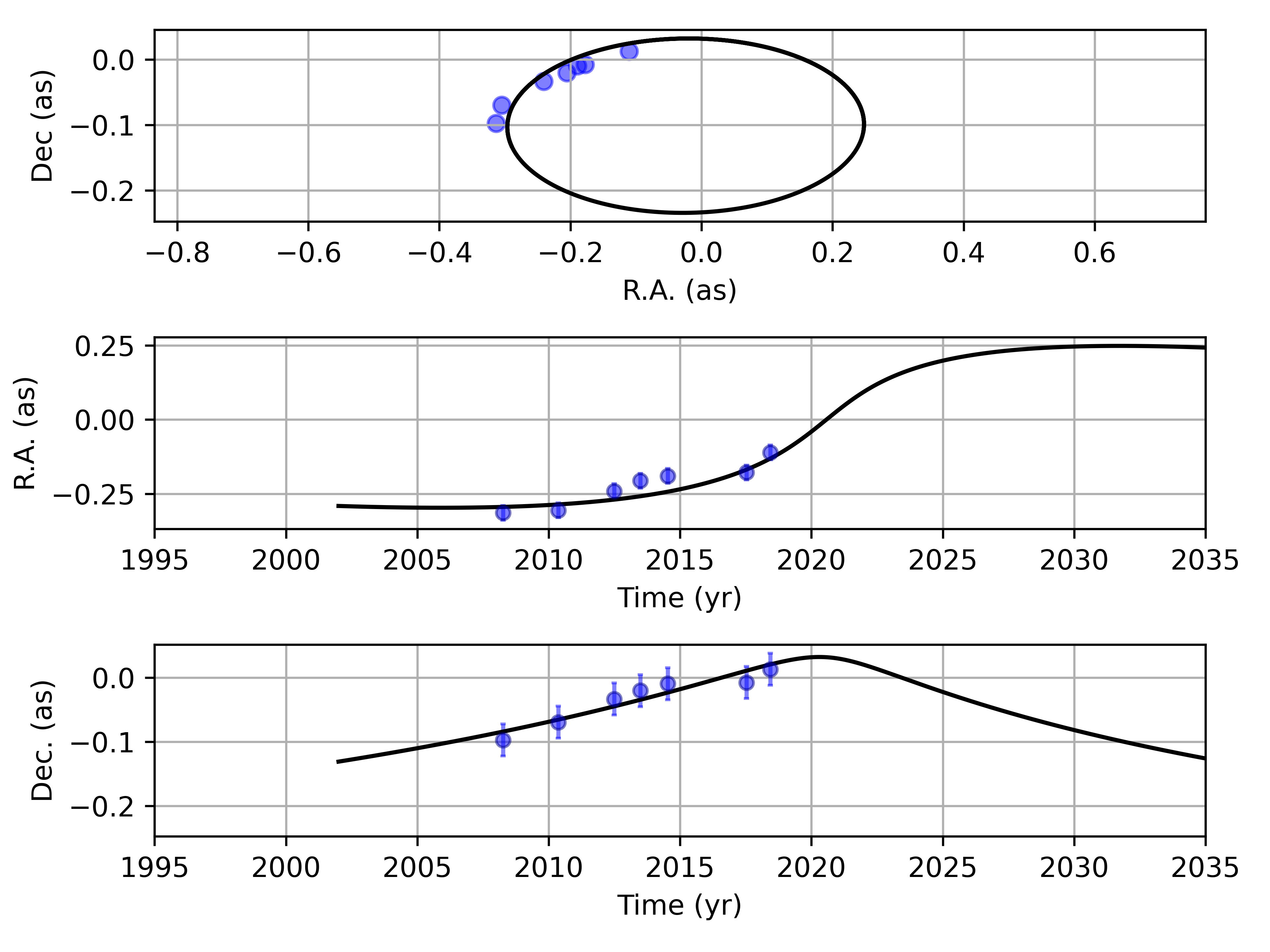
Figure 14: A Keplerian orbit of the line-emission source OS1 based on the Br$\gamma$ analysis. The pericenter passage of OS1 is dated to be around mid-2020.

In Table 7, we list the related orbital elements.

Source	$a$ (mpc)	$e$	$i$(o)	$\omega$(o)	$\Omega$(o)	tclosest(yr)
OS1	16.75 $\pm$ 0.50	0.762 $\pm$ 0.075	71.39$\pm$ 20.68	93.79 $\pm$ 8.42	271.52 $\pm$ 16.50	2020.67 $\pm$ 0.02
OS2	12.48 $\pm$ 0.19	0.605 $\pm$ 0.019	84.62 $\pm$ 4.98	140.26 $\pm$ 4.92	245.28 $\pm$ 2.17	2029.87 $\pm$ 0.05
G2/DSO	17.45 $\pm$ 0.20	0.962 $\pm$ 0.004	58.72 $\pm$ 2.40	92.81 $\pm$ 1.60	295.64 $\pm$ 1.37	2014.38 $\pm$ 0.01

Table 7: Orbital elements for the sources OS1 and OS2. For comparison, we additionally list the orbital elements of the G2/DSO (Tab. 5). The pericenter distance of OS1 and OS2 is 3.99 mpc/822 AU and 4.93 mpc/1017 AU, respectively. For comparison, the pericenter distance of the G2/DSO is 0.66 mpc/137 AU.

With $r_{\rm p}\,=\,a(1-e)$, we derive a pericenter distance of 1201.56 AU (100.08 mas) for OS1.
Please see Fig. 26 in the Appendix E for the spectral line evolution , Table 14 and Table 15 for the related positions and LOS velocities.

3.7.2 OS2

Inspecting Fig. 12 (right panel) implies that OS2 can be observed with an increased intensity count compared to OS1 in 2008. Hence, the object could be less prone to confusion due to nearby stellar sources. Given the fluctuating background in the S-cluster and the changing distance to nearby stars, the intensity difference in 2008 may not be true for every other epoch. However, using the analysing tools that we already applied to the G2/DSO and OS1, we find OS2 throughout the data approaching Sgr A* (Fig. 15).

Figure 15: Br$\gamma$ line evolution of OS2 between 2007 and 2018. Because of nearby stars, the Br$\gamma$ line is affected by stellar emission (see especially 2009). In 2012, 2013, and 2014, OS2 is isolated in relation to close-by stars. Sgr A* is indicated with a white $\times$. Here, North is up, East is to the left. The size of each panel is $0.56"\,\times\,0.50"$.

We use a Keplerian orbital fit and find with a satisfying agreement with the data a plausible solution for the trajectory of OS2 (Fig. 16).

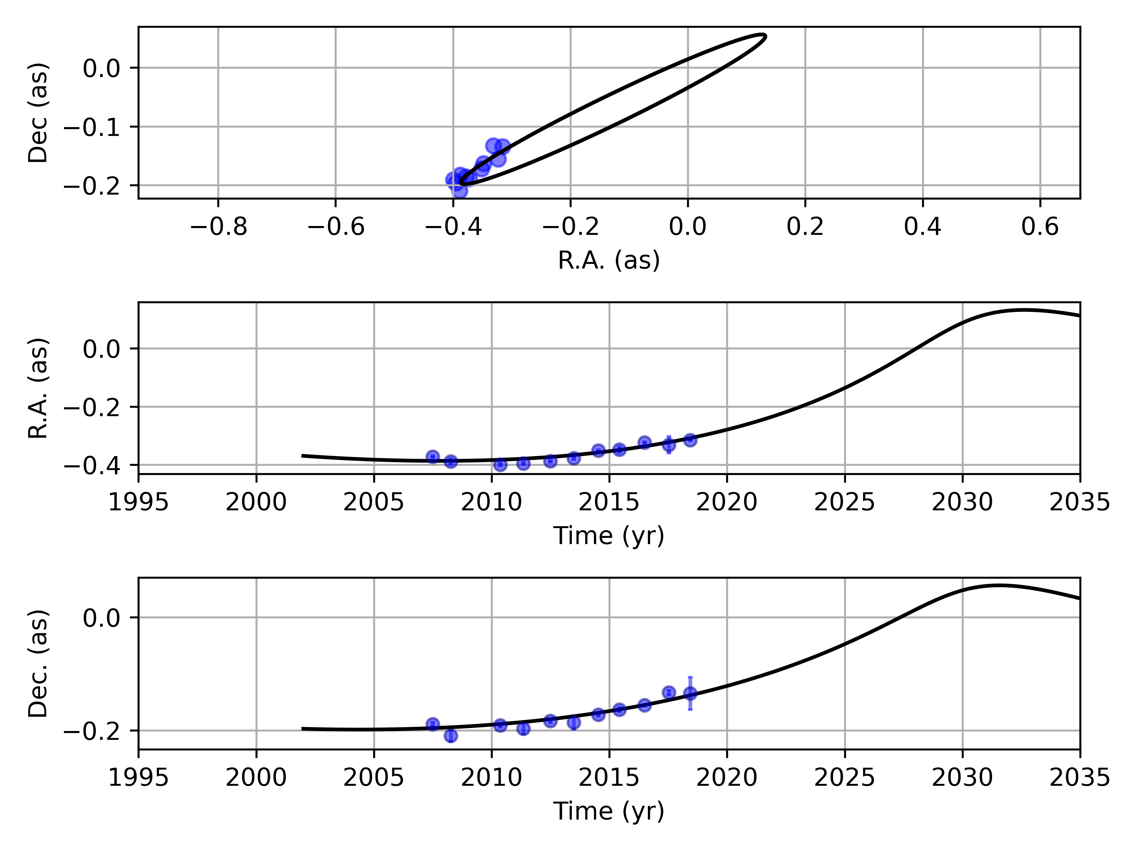
Figure 16: The orbit of OS2 as it approaches Sgr A*. Because a confusion-free detection of OS2 cannot be guaranteed in 2009, we exclude this data point from the orbital fit. We derive a periapse distance $r_{\rm p}$ of OS2 of about 13 AU in 2029.87 (see the text for details).

The related orbital elements can be found in Table 7. Using the relation for the pericenter distance, $r_{\rm p}\,=\,a(1-e)$, we calculate a pericenter distance of 1485.82 AU or 123.75 mas for OS2. In the Appendix E, in Fig. 27, we show the Doppler-shifted LOS velocity evolution (Br$\gamma$ based) with the related fit. Furthermore, we list the positions and LOS velocities in Table 14 and Table 15, respectively.

4 Discussion

In the analysis, we focused on the profound effects of sky subtraction and the smoothing on the analysis of the G2/DSO. The source is identified as compact within the measurement uncertainties both before and after the pericenter passage. The identified $K$-band counterpart supports the stellar nature of the source. The previously claimed tail emission can be disentangled into discrete sources in some epochs (OS1 and OS2). We showed that the Gaussian smoothing in noisy line maps enhances the previously claimed tail emission which instead can be disentangled into discrete sources in some epochs (OS1 and OS2) if no smoothing is applied. In the following, we will discuss the presented results and provide an answer regarding the nature of the G2/DSO.

4.1 Detection of the G2/DSO between 2005-2019

By inspecting and analyzing the SINFONI line maps, we find the G2/DSO on its Keplerian trajectory around Sgr A* between 2005 and 2019 in the Doppler-shifted Br$\gamma$ regime. The Br$\gamma$ line is less affected by tellurics but coincides with OH emission lines with a relative flux between $20\,-\,50\,\%$. As we have shown in Sec. 2 and Sec. 3, image motion but also the sky emission variability influences the analysis of the G2/DSO. While the distortions of long-time SINFONI exposure data cubes do show nonlinear inconsistencies regarding object positions (and hence impact positional uncertainties), the shape of the emission lines are affected by an insufficient sky correction. By introducing an error to the sky correction files, we find values for the velocity gradient that are twice as prominent as the observed value. Arguably, our naive approach of the sky variability may not cover every aspect of the topic since this is beyond the purpose of this analysis. Hence, it is safe to assume that this introduced error could be increased or decreased in reality.
Since the final data cubes cover a wide range of data of the related epochs, a “natural" velocity gradient is expected. However, smoothing the data leads to a velocity gradient that is twice as large as the expected value. This is awaited because of the noisy character of the SINFONI data.
Nevertheless, the confusion-free detection of the Doppler-shifted Br$\gamma$ emission line implies a Keplerian orbital evolution. The periapse of the G2/DSO can be dated to 2014.38 with a pericenter distance of about 137 AU. Comparing the line emission before and after the pericenter passage reveals a preserved shape of the observed envelope (Fig. 3), which implies that the gravitational influence of Sgr A* is in the uncertainty domain (Eckart et al., 2013). The LOS velocity follows the evolution expected for the Keplerian trajectory. Based on the Doppler-shifted G2/DSO line analysis, we find the maximum values of $v_{z}\,=\,3000\,{\rm km/s}$ (pre-periapse) and $v_{z}\,=\,3200\,{\rm km/s}$ (post-periapse) which is about $1\%$ of the speed of light. We furthermore investigated the blueshifted line maps in 2014 that should show a prominent structure as shown in Pfuhl et al. (2015). As it is already indicated in Valencia-S. et al. (2015), the line maps do not show comparable structures as it is presented in Pfuhl et al. (2015) and Plewa et al. (2017). Using a slit along the orbit in combination with a smoothing kernel and enhancing only parts of the presented image may lead to a false interpretation of the data (see Fig. 12 and Tab. 6). To underline this point, we presented nonsmoothed position-position-velocity diagrams of the G2/DSO of 2008, 2010, and 2012. In these years, the source is rather isolated in relation to nearby stars but should also exhibit a noticeable velocity gradient. However, the analysis shows a rather compact source that suffers from the background noise. In the Appendix C, in Fig. 24, we smooth the data with a 3 px Gaussian kernel. The results do show indeed some structures that could be interpreted as a possible tail structure (marked in Fig. 24, Appendix C). Unfortunately, the nonsmoothed data do not support this interpretation because of the noise. Hence, placing a slit along the orbit and smoothing the emission will most likely produce artefacts. We will investigate this point separately in detail in an upcoming publication since it would exceed the scope of this work.

4.2 Stellar counterpart of the gas emission

As it was first proposed by Murray-Clay & Loeb (2012), the presence of a stellar counterpart surrounded by a gaseous-dusty photoevaporating proto-planetary disc can explain both the ionized gas of $\sim 10^{4}\,{\rm K}$ traced by broad Br$\gamma$ emission as well as the dust component revealed by the prominent excess towards longer infrared wavelengths, in particular $L$- and $M$-bands. The color-color diagram ($H-K$ vs. $K-L$) of Eckart et al. (2013), the foreshortening factor temporal evolution presented in Valencia-S. et al. (2015), the detected polarized continuum light by Shahzamanian et al. (2016) as well as the derived SED based on the 3D dusty model by Zajaček et al. (2017) as well as Peißker et al. (2020b) all support the dust-enshrouded star model of G2/DSO. These findings are also consistent with Scoville & Burkert (2013) who suggested a supersonic low-mass T-Tauri star with a stellar wind that produces a two-layer bow-shock while interacting with the ambient hot X-ray emitting gas. In this scenario, Br$\gamma$ emission line is produced in the colder and denser stellar-wind shock via the collisional ionization at the shock front and/or the cooling X-ray/UV radiation of the post-shock gas. Additionally, Ciurlo et al. (2020) used a stellar model for the findings of the so-called G-sources which is compatible with the discussion of the same objects in Peißker et al. (2020b). Witzel et al. (2014, 2017), who also favor a dust-embedded star scenario, came to the same conclusion by analyzing the $L$-band flux density before and after the periapse of G2/DSO and G1, respectively. They found a constant flux density for G2/DSO within uncertainties, which implies the compact dust-enshrouded stellar source, while for G1 they detected a drop by nearly 2 magnitudes that can be interpreted by the tidal truncation of an extended envelope. The constant flux behavior of G2/DSO can be confirmed for its pericenter passage in this work as well. We note a slight flux increase for the data between 2018 and 2019. This could be explained by the partial removal of an envelope material during the pericenter passage where the G2/DSO host star is more revealed and as a result the overall $K$-band flux density increases. Eckart et al. (2013) suggest that the location of the Lagrange point L1 hinders a complete disruption of the envelope, since the denser component that is inside approximately one astronomical unit is bound to the star, see the tidal (Hill) radius estimate given by Eq. (3). Detailed numerical models are beyond the scope of this work but should be investigated in future works based on our findings.
Since we used a high-pass filter, we minimized the contaminating influence of overlapping PSF (-wings) and maximize the accessible information. We find a stellar counterpart at the expected position in agreement with the Br$\gamma$ emission line that is moving on the same orbit as the G2/DSO. We want to note that we already investigated the broad spectrum of results that can be derived by using a high-pass filter, see in particular the results presented in Peißker et al. (2020a). We find that a high number of iterations ($\sim\,10000$ iterations) in combination with a solid PSF can result in robust detections.
As discussed in Eckart et al. (2013) and Peißker et al. (2021a) but also shown in Sabha et al. (2012), the possibility for a side-by-side flyby becomes negligible after about 3 years. Even though the orbit of S23 and S31 interfered with the trajectory of the G2/DSO during the years 2015-2017 and 2019, we confirm the robust detection of a stellar source at the position of the G2/DSO for most of the investigated years.

4.3 The tail of G2/DSO

Several publications claim the existence of a tail component of G2/DSO that was supposed to be created because of the gravitational and hydrodynamical interaction with the environment of Sgr A*. Unfortunately, it is not clear why the tail moves on a different orbit than the head component (see Fig. 3 in Pfuhl et al., 2015). If there is a responsible process for this orbit discrepancy, we raise the question why the head is unaffected? Assuming a much higher density for the head compared to the so-called tail, it is controversially reported that G2/DSO was supposed to be destroyed during the periapse. However, Gillessen et al. (2019) reports that G2 is rather compact again after the periapse due to tidal focusing and moves on a drag-force influenced orbit. Assuming material would have been accreted by Sgr A* during the periapse of G2/DSO, the flare observed by Do et al. (2019b) could be a speculative link. However, it is also reasonable to assume, that the periapse of S2 in 2018 (Schödel et al., 2002; Do et al., 2019a) could have created instabilities in the accretion disk of Sgr A* (Suková et al., 2021) resulting in a bright flare. In contrast to the drag-force influenced orbit as proposed by Gillessen et al. (2019), we show in this work that G2/DSO follows a Keplerian trajectory where the source is not significantly affected by the tidal field of Sgr A* (see, e.g., Fig. 3). We furthermore show in Fig. 23, that the ionized gas, that is associated with the tail (Gillessen et al., 2013b) was in the S-cluster before G2/DSO passed by.
By investigating the tail, it consists rather of isolated sources that can be, like the G2/DSO, detected in the Doppler-shifted Br$\gamma$ line (see Fig. 18).

Figure 17: Combined orbit plot of the G2/DSO, OS1, and OS2 (sources are indicated in the figure). All three compact sources can clearly be separated from each other. The position of Sgr A* is located at (0,0). The black dots mark the Keplerian derived position of the related source in 2008. The fit is based on the data shown in Fig. 6, Fig. 14, and Fig. 16. We furthermore implement the LOS velocity along the orbit (see also Fig. 7, Fig. 26, and Fig. 27).

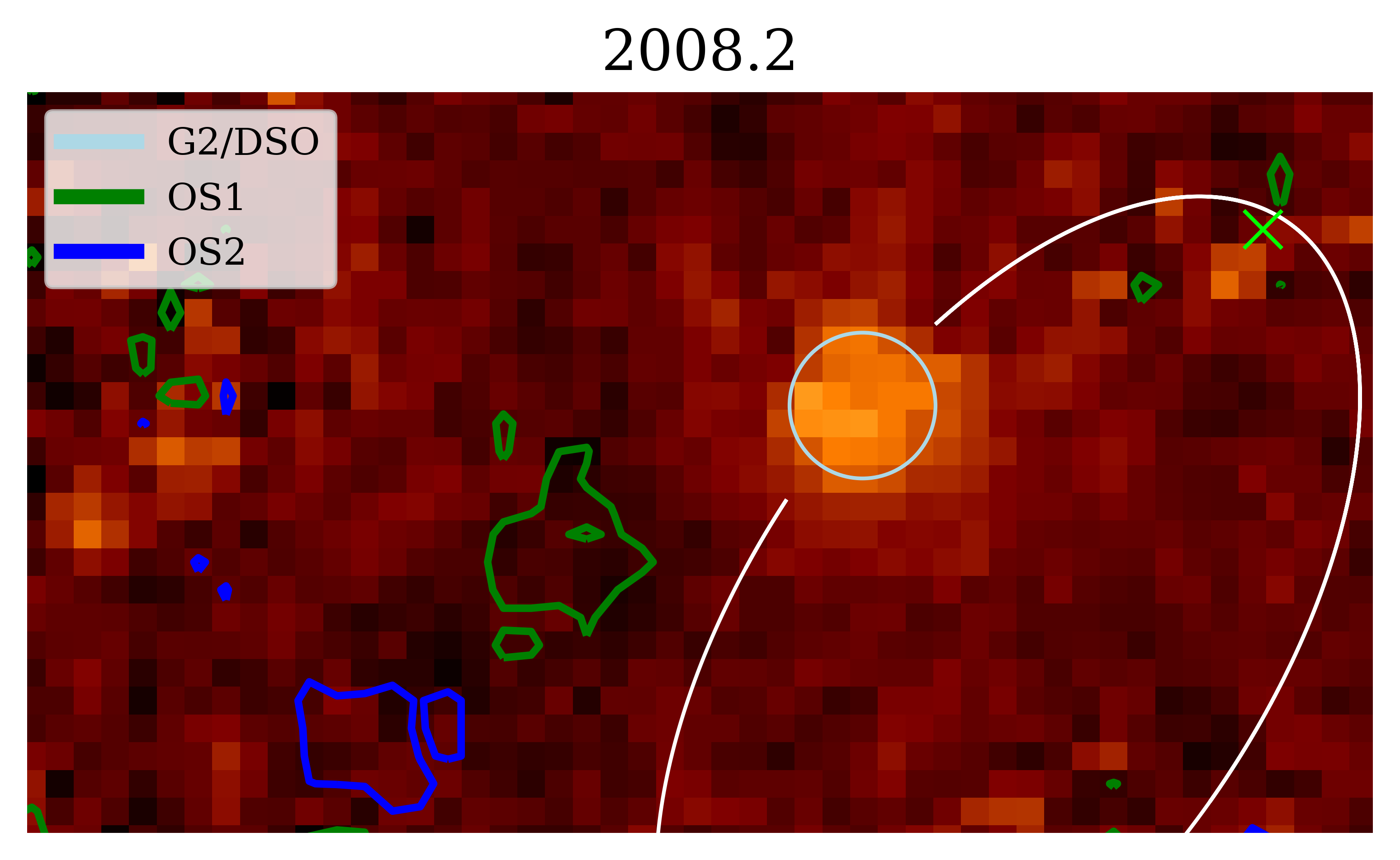
Figure 18: Doppler-shifted Br$\gamma$ line emission of G2/DSO at its velocity of about $1300$km/s and the contours of OS1 (green) and OS2 (blue) based on the data of 2008 presented in this work as shown in Fig. 13 and Fig. 15. The orbit solution is based on this work. Placing a slit over all three sources and smoothing the data results in the tail emission as shown in Fig. 12 and Fig. 24, Appendix C. In this figure, North is up, East to the left. Sgr A* is located at the lime colored $\times$. The size of the panel is $0.6\,\times\,0.3$ arcsec.

Considering the observed number of S-stars (about 40), the amount of line-emitting objects is of the same order of magnitude (almost 20). Hence, the presence of OS1 and OS2 contributes to the overall distribution of line emitting objects (for a complete overview, see Ciurlo et al., 2020; Peißker et al., 2020b).

4.4 Origin and nature of the source G2/DSO

Due to the Br$\gamma$ compactness of the object in combination with the photometric detection of a $K$-band counterpart at the position of the line-emitting source (Fig. 10 and Fig. 28, Appendix F), we find strong support for a possible young stellar object. As shown in Lada (1987), a young protostar ($<\,1\,\times\,10^{7}$ years) consists of a black-body stellar emission as well as a cooler disk/envelope component. Hence, a two-component SED fit as presented in Peißker et al. (2020b) provides a suitable explanation for the observed continuum emission and is in agreement with the predictions by Murray-Clay & Loeb (2012). Because of the ongoing accretion processes, the emission lines can show a nonsymmetric profile which is amplified by the interaction with the ambient medium, in particular by the formation of a bow shock layer (Zajaček et al., 2016; Shahzamanian et al., 2016). As pointed out by Zajaček et al. (2017), the sum of the observational results underlines the stellar nature of the object that consists of a non-spherical gaseous-dusty envelope shaped by the bow shock as well as by bipolar cavities. Hence, it is expected that the ionized gas is not centered at the source itself but exhibits an offset. Considering the mentioned bow shock layer (Zajaček et al., 2016) in combination with the polarized continuum detection (Shahzamanian et al., 2016), the proposed nature of G2/DSO as a young T-Tauri star by Scoville & Burkert (2013) and Eckart et al. (2013) seems reasonable. Furthermore, the Br$\gamma$ width variation (Fig. 25, Appendix D) of G2/DSO is in line with observations of YSOs by Stock et al. (2020) and emphasizes the proposed classification.
The pericenter passage of G2/DSO is dated to 2014.38, OS1 and OS2 are following in 2020.67 and 2029.87, respectively. Even though the orbital elements for OS1 and OS2 are different, the former source shows similarities in inclination and the argument of periapse with G2/DSO. Because of the compactness and the Doppler-shifted Br$\gamma$ line emission in combination with the missing [FeIII] detection in contrast to the D-/G-sources (see Ciurlo et al., 2020; Peißker et al., 2020b), which are located west of Sgr A*, we hypothesize if G2/DSO, OS1, and OS2 do share a common history. If so, they should have been formed in the same dynamical process. Following this speculative scenario, the combination with the detected reservoir of fast moving molecular cloudlets (Moser et al., 2017; Goicoechea et al., 2018; Hsieh et al., 2021) and the simulation of an infalling cloud presented in Jalali et al. (2014) might provide a suitable explanation for the in-situ star formation event. The authors of Jalali et al. (2014) model a $100\,M_{\odot}$ cloud that crosses the Bondi radius of Sgr A* (for observations, see also Tsuboi et al., 2018). As an initial setup, Jalali et al. (2014) assume the loss of an angular momentum via the clump-clump collisions within the CND (see also Scoville et al., 1986; Tan, 2000; Tress et al., 2020; Tartėnas & Zubovas, 2020, for the studies where molecular cloud-cloud collisions were considered). Because of the gravitational potential of Sgr A*, the initial cloud gets stretched and triggers, because of a compression force acting perpendicular to the orbital motion, the creation of YSO associations, similar to IRS13N. We will elaborate on this in more detail in Sec. 4.7.
It is rather unlikely that the G2/DSO itself was formed in the clockwise stellar disk located further out (CW disk, see Fig. 19) as, for example, claimed by Burkert et al. (2012) because of a large difference of inclinations ($i_{\rm CSD}\,\approx\,115^{\circ}\,\neq\,60^{\circ}\,\approx\,i_{\rm{G2/DSO}}$).

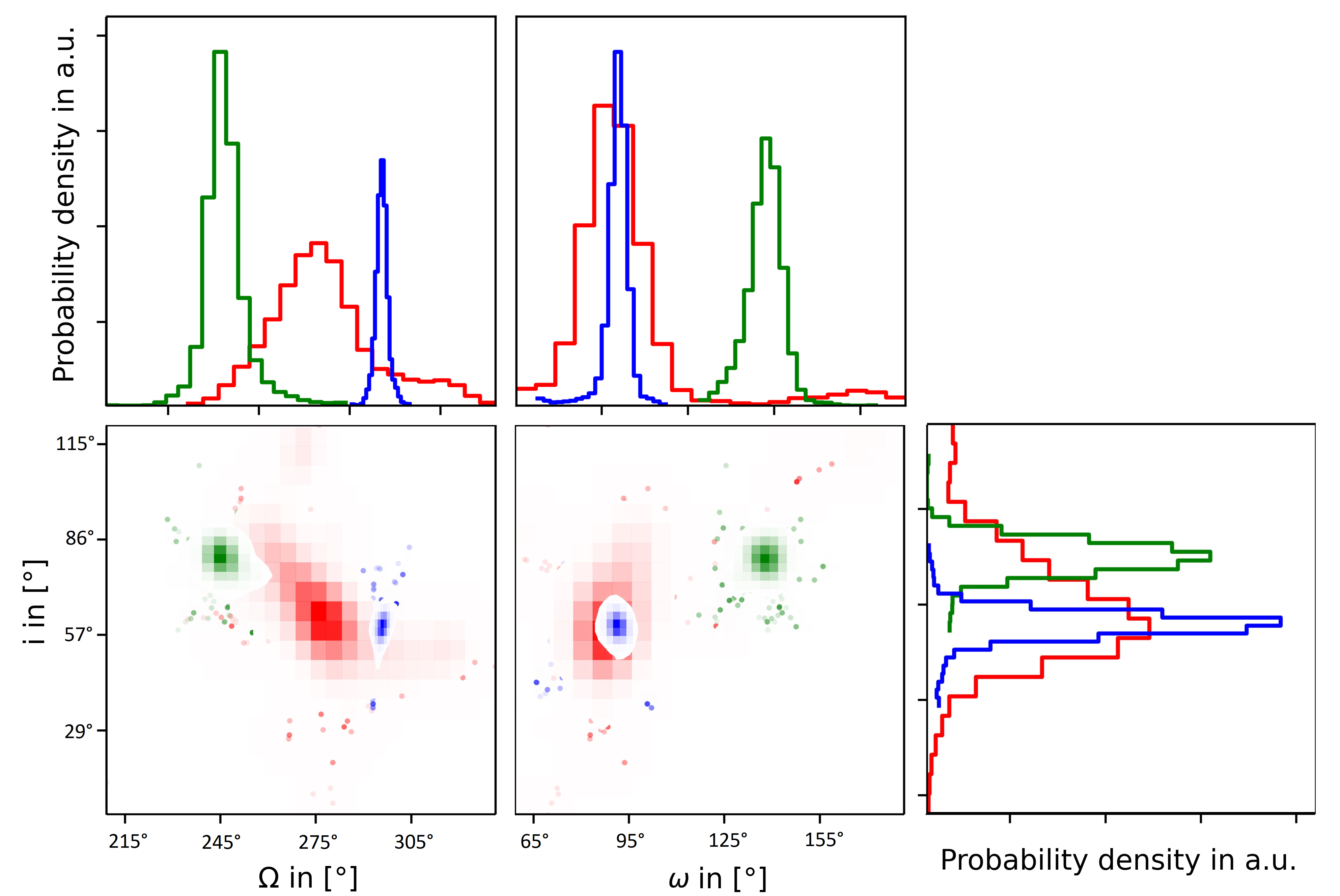
Figure 19: Inclination ($i$) as a function of the longitude of the ascending node ($\Omega$) and the argument of periapse ($\omega$). We adapt the 2d posterior distributions from Fig. 29, Fig. 30, and Fig. 31 (for every mentioned figure, please consider the Appendix G). Considering the 1-$\sigma$ interval, G2/DSO (blue) and OS1 (red) do show similarities in $\omega$ and $i$ while OS2 (green) differ. The upper two and the lower right panel (density in arbitrary units a.u.) underline a speculative common origin of the G2/DSO, OS1, and OS2. The clockwise stellar disk with $i\,=\,(90\,\pm\,10)^{\circ}$ and $\Omega\,=\,(130\,\pm\,10)^{\circ}$ is thus highly unlikely as a birthplace of the G2/DSO due to a significant offset of its mean orbital elements.

The nondetected destruction process of the source (see, e.g., Burkert et al., 2012; Schartmann et al., 2012) and the previously derived inclination of about $110^{\circ}\,-\,120^{\circ}$ for G2/DSO may be explained by the lower data baseline.

4.5 Properties of the young accreting star

By analysing the $K$-band emission of the continuum counterpart of the Doppler-shifted Br$\gamma$ line source, we find an averaged magnitude of $18.48\,\pm\,0.22$ mag with a correlated flux of $0.25\,\pm\,0.06$ mJy which matches the values presented in (Eckart et al., 2013) and Shahzamanian et al. (2016). In agreement with Sabha et al. (2012), we observe a background magnitude close to G2/DSO and as a function of the distance towards Sgr A* with a slope of $0.13$. This underlines the robust observation of the K-band magnitude observation of G2/DSO in pre-/post-periapse epochs which is not correlated to the increasing background light towards Sgr A*.
The G2/DSO passed Sgr A* in 2014.38 at a pericenter distance $r_{\rm p}$ of about 137 AU. From the foreshortening factor, which is maximized during the periapse, the true size of the G2/DSO can be inferred (Valencia-S. et al., 2015). By applying a Gaussian fit to the Br$\gamma$ line map in 2014.38 (see Fig. 3), we find a symmetrical shaped FWHM of about 37.5 mas (i.e. 3 px). Over $85\%$ of the total emission of the G2/DSO is concentrated in a very compact area with a radius of 12.5 mas in 2014.38 (see Fig. 3). In combination with the foreshortening factor, the character of the G2/DSO can be classified as compact. The authors of Scoville & Burkert (2013), Eckart et al. (2013), and Valencia-S. et al. (2015) furthermore derive a mass of $1-2\,M_{\odot}$ for the G2/DSO. From the observed averaged $K$-band magnitude in this work of $mag_{K}\,=\,18.48$ in combination with the H- and L’-band magnitude (see Eckart et al., 2013; Peißker et al., 2020b), we derive colors of $K-L\,=\,4.08$ mag and $H-K\,=\,1.48$ mag for the G2/DSO (see Fig. 20). These are common values for Herbig Ae/Be stars with ice features but also the IRS13N sources (see also Eckart et al., 2004; Moultaka et al., 2005). Recently, Cheng et al. (2020) reported matching values for observed YSOs with a circumstellar disk.

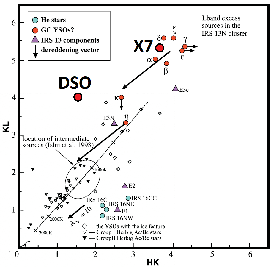
Figure 20: Young stellar objects in the GC. This figure is adapted from Ishii et al. (1998) and Eckart et al. (2004). We mark X7 (Peißker et al., 2021a) and the G2/DSO (this work).

With the upcoming Mid-Infrared Instrument (MIRI, see Bouchet et al., 2015; Rieke et al., 2015; Ressler et al., 2015) for the James Webb Space Telescope (JWST), we will be able to confirm the presence of ice features (Moultaka et al., 2015).

The estimated radius of $12.5\,{\rm mas}$ close to the pericenter passage corresponds to the upper limit on the physical length-scale of $\sim 103\,{\rm AU}$. However, the true physical size of the G2/DSO envelope is plausibly one or two orders of magnitude smaller. Using the derived pericenter distance and the G2/DSO mass estimate, we obtain the tidal radius at the pericenter of

$$r_{\rm t}^{\rm per} =a(1-e)\left(\frac{m_{\star}}{3M_{\bullet}}\right)^{1/3}\,$$

$$\sim 0.6\,\left(\frac{m_{\star}}{1\,M_{\odot}}\right)^{1/3}{\rm AU}\,.$$ (3)

Given the orbital period of the G2/DSO, $P_{\rm orb}\sim 105\,{\rm yrs}$, the source likely went through several pericenter passages, possibly thousands in case of a stellar nature. Therefore, the length scale of the G2/DSO is likely small, of the order as expressed by Eq. 3, which makes the source interesting from the point of view of stellar evolution and extreme star formation. The 3D MCMC radiative transfer simulations performed by Zajaček et al. (2017) showed that the basic continuum properties of the source can be reproduced with the compact gaseous and dusty envelope of the order of an astronomical unit. The constant $L$-band (Witzel et al., 2014) as well as $K$-band flux density (this work) implies that the tidal prolongation and truncation of the envelope has rather been small, which is in contrast to the G1 source (Witzel et al., 2017) that has exhibited profound SED changes in the post-pericenter phase. The recent increase in the $K$-band flux density after 2017, see Fig. 11, may indicate changes in the envelope morphology, however, this will need to be clarified with more post-pericenter $L$- and $K$-band data. In conclusion, the length-scale of the G2/DSO has been $\sim 1\,{\rm AU}$ both before and after the pericenter passage.

4.5.1 Br$\gamma$ line width of the G2/DSO

As proposed by, e.g. Gillessen et al. (2019), the increasing line width of the Doppler-shifted Br$\gamma$ emission of the G2/DSO until 2014 could be interpreted via the tidal stretching of the extended cloud. The decreasing line width after 2014 was proposed to be due to the tidal focusing (Gillessen et al., 2019).

Eckart et al. (2013), Zajaček et al. (2016), and Shahzamanian et al. (2017) consider a dust-enshrouded star to explain the observations of the G2/DSO. As shown by Valencia-S. et al. (2015) and this work, a variation of the Br$\gamma$ line width is detectable in the data sets that cover 2005 to 2019. In contrast to the pure cloudy nature of the source, we consider an internal and external explanation for the line width variation. Hence, the observed Br$\gamma$ emission line width could be produced by two proposed mechanisms:

• The production within the denser and colder stellar wind bow shock due to the collisional ionization (Scoville & Burkert, 2013). As was explicitly shown by Zajaček et al. (2016), due to the variable viewing angle of the bow-shock velocity field with respect to the observer, the line width increases from $\sim 100\,{\rm km\,s^{-1}}$ up to $\sim 200\,{\rm km\,s^{-1}}$ at the pericenter passage ($2014.4$) and then decreases down to $\sim 100\,{\rm km\,s^{-1}}$ in the post-pericenter phase, see in particular the comparison of the model calculations with the observed line width in Fig. 5 (orange and black lines for the case with no outflow and an outflow of 2000 km/s, respectively),

• a broad Br$\gamma$ line with the line width of a few 100 km/s is commonly detected in young YSOs of class I, and can be produced within the disc winds and/or in the process of magnetospheric accretion (Valencia-S. et al., 2015; Stock et al., 2020).

We have shown in Fig. 5 that the line width between 2006 and 2008 is rather decreasing. Considering also the absence of a tail emission (Fig. 8, 9, 12, 23, 24), we strongly question a tidal stretching scenario. Because of the ongoing accretion from the host star (Murray-Clay & Loeb, 2012; Scoville & Burkert, 2013; Zajaček et al., 2016), an overall trend can be observed and shows the same behavior as the foreshortening factor (Valencia-S. et al., 2015). In particular, we pay attention to the outliers in 2014.3 and 2015.4. The width of the Br$\gamma$ line of the G2/DSO at $2.1490\,{\rm\mu m}$ in 2015.4 and $2.1857\,{\rm\mu m}$ is polluted by the strong OH emission at $2.1505\,{\rm\mu m}$, $2.1507\,{\rm\mu m}$, and $2.1873\,{\rm\mu m}$ (Rousselot et al., 2000). Inspecting the presented spectrum in Fig. 4 reveals peaks that significantly broaden the Doppler-shifted G2/DSO Br$\gamma$ line in 2014.3 and 2015.4 at $2.1874\,\mu m$ and $2.1509\,\mu m$, respectively. Effectively, this broadening is due to the OH line emission (see Sec. 2.8) and increases the line width in 2014.3 and 2015.4 by about $30\%$. By applying this correction, we derive a line width of 234 km/s and 243 km/s for the G2/DSO in 2014.3 and 2015.4, respectively.
Based on the measured line map size (Table 4), the true size of the G2/DSO can be observed at the pericenter passage in 2014.38. Since the evolution of the line width coincides with the foreshortening factor trend (see Valencia-S. et al., 2015), we can safely assume that the observed effect is due to the stellar nature and the orientation of the source.

4.6 Magnetohydrodynamic drag force

Pfuhl et al. (2015) discussed and showed a possible drag force acting on the G2/DSO. Within this model, the authors combined the data of G1 and G2/DSO to demonstrate the effect of the predicted inspiraling cloud towards Sgr A* after the pericenter passage (see, e.g., Gillessen et al., 2012). In Fig. 21, we compare the predicted trajectory of G2/DSO that is following G1 as part of a gas streamr (Pfuhl et al., 2015) with the observed data (black data points) and the derived orbit.

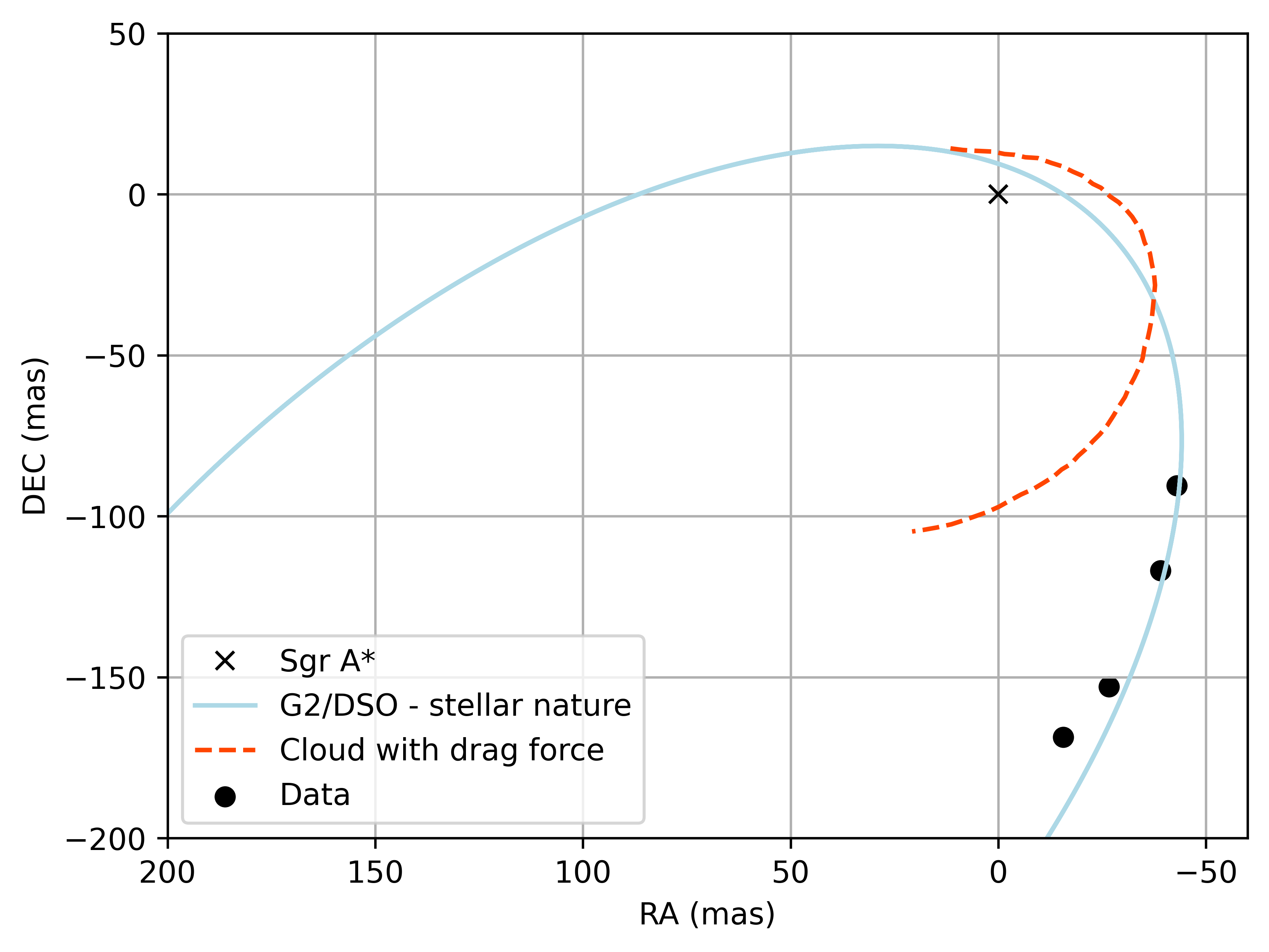
Figure 21: Based on the proposed gas streamer idea of Pfuhl et al. (2015), the authors connect the orbit of G1 and G2/DSO to predict the evolution of the gas cloud (red dotted line). Comparing the Br$\gamma$ position of the G2/DSO after the periapse between 2016-2019 with the gas-streamer idea reveals gaps between the proposed evolution and the observed trajectory as shown by the blue line.

The comparison indicates that no measurable drag force as proposed by Pfuhl et al. (2015) can be observed and its assumption, that G2/DSO is part of a gas streamer cannot be confirmed. In comparison to Pfuhl et al., the magnetohydrodynamic drag force analysis by Gillessen et al. (2019) discusses a smaller drag force with respect to the pre-pericenter orbit of G2/DSO. However, the hardly recognizable presented effect is underlined by shortening the observational available pre-pericenter data points in the related publication of Gillessen et al. (2019) (see their Fig. 2). When we consider all available SINFONI data up to 2019, the position- and velocity-data can simultaneously be fit well with a simple Keplerian orbital solution, see Fig. 6 and Fig. 7. Following Occam’s razor (see, e.g., Ariew, 1976), the inclusion of an additional drag term appears redundant. Moreover, we have shown that the influence of image motion (Tab. 1) and sky variability can have a significant impact on the data by up to $40\%$. Based on the data presented in Gillessen et al. (2019), we conclude that the arguably small offset (< few percent) of the Br$\gamma$ source in combination with the presented line shape might not be explained by a drag force and can rather be explained by the effects discussed in this work. By carefully inspecting the provided Kepler- and Drag Force-fits in Gillessen et al. we note, that both models do not perfectly match the shown Br$\gamma$ emission which underlines the noisy character of the SINFONI data. Based on these points, we do not find a strong need for a drag force to explain the orbital evolution of the G2/DSO (Fig. 3). In a similar way, Witzel et al. (2017) found that the evolution of G1 is consistent with the Keplerian motion on a different highly-eccentric orbit to that of the G2/DSO, which supports the stellar nature of both sources. In this regard, the tests of alternative gravitational theories, such as the fermionic dark matter compact core–diffuse halo (Becerra-Vergara et al., 2020), that has made use of the G2/DSO orbit should be updated accordingly.

4.7 Are the G2/DSO, OS1, and OS2 YSOs or rather related to the stellar binary dynamics?

In Zajaček et al. (2014), the authors propose the possibility that the G2/DSO can be associated with a binary or multiple-star dynamics close to the Galactic center. In particular, they showed that in case the G2/DSO is a binary system, it would lead to the disruption event at the pericenter. This model was soon followed by scenarios that explain the G2/DSO and related objects as binary merger products (Perets et al., 2007; Stephan et al., 2016, 2019). Following the binary merger fraction discussion of Ciurlo et al. (2020), we adapt

$$R\,=\,\frac{1}{2}\frac{N_{B}}{N_{m}}$$ (4)

from this publication and assume, that line emitting and dusty objects are binary merger products. By using this equation, the binary fraction R is calculated with the number of binaries $N_{B}$ and the number of low-mass stars $N_{m}$. To provide a certain degree of comparability, we adapt $N_{m}\,=\,478$ from Ciurlo et al. and consider the additional sources from Peißker et al. (2020b) which results in $N_{B}\,=\,85$. For R, we derive $\sim\,9\%$ which is almost twice as much as the binary fraction of $\sim\,5\%$ calculated in Ciurlo et al. (2020). Since we assumed that all objects are binary merger, it is safe to conclude that the assumption is not justified. We obtain a low-mass binary fraction that is almost twice than that derived by Ciurlo et al. and also larger than the overall predicted value of $6-7\%$ (Raghavan et al., 2010; Stephan et al., 2019; Ciurlo et al., 2020). Hence, we conclude that a considerable fraction of the overall population of line and dust emitting sources are not necessarily binary mergers but also YSOs. We would like to emphasize that a binary merger scenario for G2/DSO is not excluded from the overall discussion.
Assuming a speculative binary disruption scenario, the pericenter passage at a unspecified time of the G2/DSO would have been responsible for the tidal break-up of the binary components that we denote here as G2/DSO₁ and G2/DSO₂. In this regard, G2/DSO₂ is a runaway star, while G2/DSO₁ is a highly eccentric component which is following a slightly modified Keplerian trajectory (Hills, 1988) with a smaller eccentricity as well as a semi-major axis (Zajaček et al., 2014). Following this, the post-pericenter trajectory of G2/DSO₁ could mimic the inspiral due to the drag force (Gillessen et al., 2019). If we consider the second star (G2/DSO₂), the magnitude of this component is at most $18.5$ mag. Because of the preserved Br$\gamma$ shape in the post-periapse years of the observed G2/DSO₁, we are allowed to speculate that G2/DSO₂ did not capture most of the surrounding stellar material. This implies a mass estimate of G2/DSO${}_{1}\,>\,$G2/DSO₂. With the derived mass for the G2/DSO of about $1-2\,M_{\odot}$, we assume that an upper limit for the mass of G2/DSO₂ is closer to $m_{\rm{G2/DSO}_{2}}\,<\,1\,M_{\odot}$.

We note that the disruption scenario applies also to the theory of in-situ star formation, where an infalling cloud that is stretched and compressed forms associations of young stellar objects (Jalali et al., 2014). These associations are first bound systems with a certain velocity dispersion. In case they orbit the SMBH on an eccentric orbit, the tidal radius of the YSO cluster is time-variable depending on the distance from the SMBH. In particular, the tidal (Hill) radius during the pericenter passage is

$$r_{\rm t}^{\rm cluster} =\overline{a}(1-\overline{e})\left(\frac{m_{\rm cluster}}{3M_{\bullet}}\right)^{1/3}\,$$

$$\sim 14.4\,\left(\frac{\overline{a}}{15.6\,{\rm mpc}}\right)\left(\frac{\overline{e}}{0.78}\right)\left(\frac{m_{\rm cluster}}{100\,M_{\odot}}\right)^{1/3}\,{\rm AU}\,,$$ (5)

where we considered the mean values of the semi-major axis and the eccentricity based on G2/DSO, OS1, and OS2 (see Table 7). The cluster mass was scaled to the order of magnitude considered in the simulations of Jalali et al. (2014) for an infalling molecular cloud. Since the YSO cluster length-scale approximately given by the Jeans length-scale for a given critical density for self-gravitation is larger than $r_{\rm t}^{\rm cluster}$, the cluster is effectively dissolved at the distances where dusty orbits are seen to orbit now. Hence, during the pericenter passage, the cluster will tend to dissociate and lose its members that will afterwards orbit around Sgr A* on independent orbits with similar orbital elements initially (inclination, longitude of the ascending node, argument of the pericenter). Due to the resonant relaxation and the perturbative effects of the S cluster as well as Newtonian (mass) and Schwarzschild precession, the inclination as well as other orbital elements will start to deviate. In this regard, G2/DSO, OS1, OS2, as well as other dusty objects can share a common origin, despite certain offsets in the orbital elements, see Table 7 and Fig. 19 for comparison.

To estimate how much individual dynamical processes can alter orbital elements of interest (inclination, longitude of the ascending node, argument of the pericenter), we compare their fundamental timescales with the assumed lifetime of the dusty sources of $\sim 10^{5}\,{\rm yr}$. In particular, the argument of pericenter shift between mainly G2/DSO and OS2 could be explained by the Schwarzschild precession, which per orbit can be estimated as follows,

$$\Delta\phi=\frac{6\pi GM_{\bullet}}{c^{2}a_{\rm G2}(1-e_{\rm G2}^{2})}$$ (6)

which for the G2/DSO yields $\Delta\phi=9.52^{\prime}$ per orbital period ($P_{\rm G2}\sim 108$ years). The difference for the argument of periapse of $\sim 50^{\circ}$ between OS2 and G2/DSO (see Fig. 19) could thus be achieved in $\sim 35\,000$ years due to the much faster prograde relativistic precession of G2/DSO than OS2 ($\sim 1.57^{\prime}$ per its orbital period). The Newtonian (retrograde) mass precession counter-balances the relativistic precession and acts in an opposite direction. The mass coherence timescale $T_{\rm c}^{M}$, on which the arguments of the periapse would be randomized, can be estimated as,

$$T_{\rm c}^{M} \sim\frac{M_{\bullet}}{<M_{\star}>}\frac{P_{\rm G2}}{N_{\star}}\,$$

$$\sim 4\times 10^{5}\left(\frac{<M_{\star}>}{10\,M_{\odot}}\right)^{-1}\left(\frac{P_{\rm G2}}{100\,{\rm yr}}\right)\left(\frac{N_{\star}}{100}\right)^{-1}\,{\rm yr},$$ (7)

where $<M_{\star}>$ is the mean stellar mass, $P_{\rm G2}$ is the orbital period of G2/DSO, and $N_{\star}$ is the number of stars inside its orbit. If the lifetime of G2/DSO, OS1, and OS2 is at most $\sim 10^{5}\,{\rm yr}$, then the mass precession has not significantly altered their orbital orientations.

The resonant relaxation process, which is characteristic of highly symmetric potentials, such as inside the sphere of influence of Sgr A*, proceeds in two modes: a faster vector resonant relaxation (VRR) and a slower scalar resonant relaxation (SRR). The VRR relaxation timescale is

$$T_{\rm VRR} \sim\frac{M_{\bullet}}{<M_{\star}>}\frac{P_{\rm G2}}{\sqrt{N_{\star}}}\,$$

$$\sim 4\,\left(\frac{<M_{\star}>}{10\,M_{\odot}}\right)^{-1}\left(\frac{P_{\rm G2}}{100\,{\rm yr}}\right)\left(\frac{N_{\star}}{100}\right)^{-1/2}{\rm Myr}\,,$$ (8)

while the SRR relaxation, which also changes the magnitude of the angular momentum is about 10 times slower because of the definition of the scalar relaxation time, $T_{\rm SRR}\sim P_{\rm G2}M_{\bullet}/<M_{\star}>$ (see Hopman & Alexander, 2006; Alexander, 2017, for details). In case G2/DSO, OS1, and OS2 were formed approximately in the same orbital plane $\sim 10^{5}$ years ago, then the VRR has not had enough time to randomize their orbits, but it could have contributed to the $\sim 20^{\circ}$ spread in orbital inclinations over time.

In terms of the deviations in the longitude of the ascending node, the orbital precession can be relevant, especially when the stellar motion is perturbed by the presence of an inclined massive stellar disk. Ali et al. (2020) revealed that the S cluster consists of at least two perpendicular stellar disks, which indicates a non-randomized stellar distribution. Beyond the S cluster, at the radius of $R_{\rm d}\sim 0.1\,{\rm pc}$, there is a stellar disc of about hundred OB stars, with the potential total mass of $M_{\rm d}\sim 10000\,M_{\odot}$ (Paumard et al., 2006; Bartko et al., 2009). If the G2/DSO infrared source is inclined by $\beta\sim 60^{\circ}$ with respect to the disc plane, the stellar disk induces torques on the misaligned dust-enshrouded objects, which then precess with a certain period $T_{\rm prec}$ around the symmetry axis, effectively shifting the line of nodes. The rate of this shift depends on the semi-major axis $a_{\star}$ and since $a_{\rm G2}=0.01745\,{\rm pc}<R_{\rm d}\sim 0.1\,{\rm pc}$, one can use the following analytical formula to estimate the stellar precession period with respect to the disc (Nayakshin, 2005; Löckmann et al., 2008),

$$T_{\rm prec}\simeq\frac{8\pi M_{\bullet}}{3M_{\rm d}\cos{\beta}}\sqrt{\frac{a_{\star}^{3}}{GM_{\bullet}}}\frac{(a_{\star}^{2}+R_{\rm d}^{2})^{5/2}}{a_{\star}^{3}R_{\rm d}^{2}}\,,$$ (9)

For the G2/DSO, the precession period can be estimated to be $T_{\rm p}\sim 2.34\times 10^{7}\,{\rm yr}$, hence it is a slow process, which leads to the shift of $\sim 1.5$ degrees in terms of the argument of the ascending node during $10^{5}$ years or $\sim 10.8$ degrees in $700\,000$ years. For OS2 the precession shift is slightly smaller than for G2/DSO and OS1, $\sim 1$ degree per $100\,000$ years, which could have contributed to the ascending node offset of $\sim 6$ degrees during the last million years. Hence, most of the difference in the ascending node is potentially attributable to the intrinsic dispersion during the formation process.

Finally, the presence of a perturbing stellar disk at the scale of $R_{\rm d}\sim 0.1\,{\rm pc}$ with the mass of $M_{\rm d}\sim 10^{4}\,M_{\odot}$ induces a Kozai-Lidov (KL) oscillations of eccentricity and the inclination. The period of the KL cycle can be estimated as (Šubr & Karas, 2005),

$$T_{\rm KL}=2\pi\left(\frac{M_{\bullet}}{M_{\rm d}}\right)\left(\frac{R_{\rm d}}{a_{\rm G2}}\right)^{3}P_{\rm G2}\,,$$ (10)

which yields $T_{\rm KL}\sim 4.73\times 10^{7}$ years. Since the timescale is about two orders of magnitude longer than the assumed lifetime of dust-embedded sources, the KL effect can slightly contribute to the above-mentioned effects to account for the overall offset of orbital elements.

Since all relevant dynamical processes operate on longer timescales than the assumed lifetime of dust-enshrouded stars, most of the offset among orbital elements reflects the way they formed - i.e. from a turbulent fragmenting molecular cloud with an intrinsic offset due to a velocity disperion, or G2/DSO and OS1 formed initially as a binary that disrupted, with OS2 forming separately as a single star. More detailed numerical dynamical studies are beyond the scope of this study.

In the binary merger scenario, the two components of a binary star initially orbit the SMBH, which acts as a more distant perturber. The SMBH as a perturber would induce Kozai-Lidov (Kozai, 1962; Lidov, 1962; Naoz, 2016) resonances of the two components, where during one cycle the eccentricity growth is exchanged for the inclination decrease and vice versa. Finally, at large orbital eccentricities, the two components are tidally distorted, induce torques on each other, and both stars are finally driven to merge. Such a merger product contracts on a Kelvin-Helmholtz timescale and is often associated with optically thick dusty outflows that give rise to the NIR-excess (Stephan et al., 2016, 2019). Hence, because of the resemblance to young stellar objects, it is difficult to distinguish between binary mergers and pre-main-sequence stars merely based on the photometry and the spectroscopy of the sources. Moreover, as mentioned before, the SINFONI data suffers from noisy behavior. Hence, the observational indications to verify a merger scenario are rather challenging to determine.

One distinguishing feature between YSOs that formed in situ in a single star formation event and dust-enshrouded merger products could be their distribution of orbital elements. While for YSOs we expect comparable orbital elements on timescales less than the resonant relaxation timescale within the S cluster, binary mergers should not follow such a condition as they form continuously and on different orbits. Since G2/DSO and OS1 share comparable orbital elements in terms of their inclination, semi-major axis, and the argument of the pericenter, see also Fig. 19, the common origin in the same star formation event is plausible. Following this argument implies that OS2 might be a binary merger. This would be fully compatible with the discussed infalling cloud scenario since Jalali et al. (2014) predicts that a certain fraction of the resulting sources are binaries and single low- and high-mass YSOs (Yusef-Zadeh et al., 2013a; Ciurlo et al., 2020; Peißker et al., 2020b).

4.8 Dust-enshrouded objects as remnants of a disrupted young stellar association

Combining some of the mechanisms discussed in the previous subsection, we hypothesize that G2/DSO, OS1, and OS2 as well as other dust-enshrouded objects could be remnant YSOs captured by the SMBH during a nearly parabolic infall of a young star cluster formed further away at the scales of $\sim 1\,{\rm pc}$ and beyond.

The advantage of this scenario is that larger distances from the SMBH put only moderate restrictions on the critical Roche density necessary for the molecular cloud to withstand disruptive tidal forces. The lower limit on the number density of the self-gravitating cloud at the distance $r$ from Sgr A* is,

$$n_{\rm cloud} \gtrsim\frac{3M_{\bullet}}{2\pi\mu m_{\rm p}r^{3}}\,$$

$$\sim 7.7\times 10^{7}\left(\frac{M_{\bullet}}{4\times 10^{6}\,M_{\odot}}\right)\left(\frac{r}{1\,{\rm pc}}\right)^{-3}\,{\rm cm^{-3}}\,.$$ (11)

In comparison, the Roche limit according to Eq. (11) within the S cluster ($\sim 0.01$ pc) gives as much as $n_{\rm cloud}>10^{14}\,{\rm cm^{-3}}$.

The critical density for the star-formation to take place could be reached via cloud-cloud collisions (Scoville et al., 1986; Tan, 2000; Tan & McKee, 2004; Hobbs & Nayakshin, 2009) within the circum-nuclear disk (CND), where individual clumps have $\sim 10^{6}-10^{8}\,{\rm cm^{-3}}$ (Hsieh et al., 2021). A further enhancement in the density can be provided by UV radiation pressure originating in NSC OB stars at the inner rim of the CND (Yusef-Zadeh et al., 2013b). Moreover, fast stellar winds and occasional supernova explosions can be another source of a star-formation trigger. External pressure is necessary for individual clumps to overcome the turbulent pressure, which prevents them from collapsing (Hsieh et al., 2021). Clump-clump collisions can partially remove the angular momentum, which helps to set the resulting self-gravitating cloud on the infalling trajectory towards Sgr A* with a small impact parameter (Jalali et al., 2014; Tress et al., 2020; Tartėnas & Zubovas, 2020). However, the overall hydrodynamics of clump-clump interactions is rather complex and only a fraction of such collisions may end up with a self-gravitating and fragmenting cloud complex falling radially towards Sgr A*. First, this is due to the complex internal structure of molecular clumps, in particular their turbulent field (Salas et al., 2021), and hence the “hard ball” approximation does not apply to them. Second, the clumps at larger distances from Sgr A*, beyond $\sim 2$ pc, follow the Galactic rotation and thus have a larger angular momentum with respect to Sgr A*, which needs to be removed for the cloud to fall in with a sufficiently small impact parameter. These two points imply that the shearing likely takes place, which can result in a formation of a new cloud without a sufficient loss of the angular momentum or a sheared gaseous streamer. The formation of shearing gaseous streamers from a set of clumps was demonstrated in the 3D N-body/smoothed particle hydrodynamics (SPH) simulations by Salas et al. (2021). In their work, the turbulence was continually injected to mimick the effect of supernovae and stellar winds. In this way, the high dispersion of the gas within the Central Molecular Zone (CMZ) can effectively be reproduced. As shown by Salas et al. (2021), the injected turbulence results in the accretion to smaller scales down to Sgr A* in the form of turbulent accretion flows (Salas et al., 2020) or high-density spiral streamers (Dinh et al., 2021). Regardless of this complex behaviour within the CMZ, for simplicity here we assume that at least once in every $\sim 10^{6}\,{\rm yr}$ (Wardle & Yusef-Zadeh, 2008; Jalali et al., 2014) a fragmenting star-forming cloud can reach the vicinity of Sgr A* with the impact parameter at the length-scale of the S cluster, where it is expected to tidally disintegrate, with a fraction of YSOs being captured by Sgr A* (Gould & Quillen, 2003), while the remaining fraction being unbound on hyperbolic orbits (Fragione et al., 2017). If the molecular cloud size is comparable or larger than its impact parameter, it can completely engulf Sgr A* and leave behind a compact star-forming disk (Wardle & Yusef-Zadeh, 2008), which may help explain the multi-disk configuration of the S-cluster (Ali et al., 2020).

The crucial point of the “infalling-cloud” model is that YSOs of the age of $\sim 10^{5}$ years can already be formed during the infall phase. Thus, we require that the infall timescale of the cloud towards Sgr A*, which is half of the orbital timescale, $t_{\rm infall}=P_{\rm orb}/2$, is longer than the free-fall timescale of the clump with the critical density $n_{\rm cloud}$, $t_{\rm ff}=[3\pi/(32G\mu m_{\rm p}n_{\rm cloud})]^{1/2}$. Hence, we obtain the lower limit on the initial distance of an infalling cloud,

$$d_{\rm cloud} \gtrsim\left(\frac{3M_{\bullet}}{32\pi\mu m_{\rm p}n_{\rm cloud}}\right)^{1/3}\,$$

$$\sim 0.4\,\left(\frac{M_{\bullet}}{4\times 10^{6}\,M_{\odot}}\right)^{1/3}\left(\frac{n_{\rm cloud}}{10^{8}\,{\rm cm^{-3}}}\right)^{-1/3}{\rm pc}\,,$$ (12)

for the free-fall timescale of $t_{\rm ff}\sim 5000$ years, which can, however, get smaller as the density within the fragmenting clumps increases beyond the limit given by Eq. (11). The outer distance range can be inferred from the G2/DSO lifetime of $t_{\rm{G2/DSO}}\sim 10^{5}\,{\rm yr}$ and from the condition $t_{\rm infall}\lesssim t_{\rm{G2/DSO}}$,

$$d_{\rm out} \lesssim(GM_{\bullet})^{1/3}\left(\frac{t_{\rm{G2/DSO}}}{\pi}\right)^{2/3}\,$$

$$\sim 2.6\left(\frac{M_{\bullet}}{4\times 10^{6}\,M_{\odot}}\right)^{1/3}\left(\frac{t_{\rm{G2/DSO}}}{10^{5}\,{\rm yr}}\right)^{2/3}\,{\rm pc}\,.$$ (13)

Given the distance range between $0.4\,{\rm pc}$ and $2.6\,{\rm pc}$, it is quite plausible that the self-gravitating cloud was formed or rather triggered towards star-formation by external pressure within the CND, which is located between $\sim 1.5\,{\rm pc}$ and $\sim 3-4\,{\rm pc}$ (Christopher et al., 2005).

In the further discussion, we analyze the scenario where the self-gravitating cloud from the CND fragmented into a cluster of pre-main-sequence stars on its way towards Sgr A*. We assume the mass of this minicluster or rather a young stellar association of $m_{\star}=100\,M_{\odot}$, which is in the range of masses of $0.05\,{\rm pc}-0.2\,{\rm pc}$ clumps within the CND (Hsieh et al., 2021). The stellar velocity dispersion is adopted from the IRS 13N association of young stars, $\sigma_{\star}\sim 50\,{\rm km\,s^{-1}}$ (Mužić et al., 2008). Then from the virial theorem, we obtain the stellar association radius of

$$r_{\star}=0.2\,\left(\frac{m_{\star}}{100\,M_{\odot}}\right)\left(\frac{\sigma_{\star}}{50\,{\rm km\,s^{-1}}}\right)^{-2}\,{\rm mpc}\,.$$ (14)

The young stellar cluster on a highly eccentric orbit will dissociate at the tidal disruption radius that can be expressed as

$$r_{\rm dis} =r_{\star}\left(\frac{M_{\bullet}}{m_{\star}}\right)^{1/3}=\,$$

$$=\frac{GM_{\bullet}^{1/3}m_{\star}^{2/3}}{\sigma_{\star}^{2}}=\,$$

$$\sim 1214\,\left(\frac{m_{\star}}{100\,M_{\odot}}\right)^{2/3}\left(\frac{\sigma_{\star}}{50\,{\rm km\,s^{-1}}}\right)^{-2}\,{\rm AU}\,,$$ (15)

which is close to the pericenter distances of OS1 and OS2, as well as other dusty sources (Peißker et al., 2020b). A few stars from an infalling cluster will remain bound to the SMBH (Gould & Quillen, 2003), while others will escape the NSC altogether as hypervelocity stars (Fragione et al., 2017). The high eccentricity of the G2/DSO as well as G1 implies that they might have been constituents of binary systems within the cluster, while the other components escaped (Zajaček et al., 2014). However, given a nearly radial infall of the cluster and its velocity dispersion, a fraction of YSOs should anyway reach the pericenter distance of the G2/DSO ($\sim 137\,{\rm AU}$) during the disruption event (see also Gould & Quillen, 2003, for statistical estimates of a similar scenario for S2 star). The detailed numerical modelling of such a cluster dissociation is beyond the scope of the paper.

Hence, once two clumps within the CND collide or there is another external trigger (intense UV radiation, supernova blast wave, collision with a jet), the clump of several $100\,M_{\odot}$ will start collapsing and fragmenting into protostars on the scale of several thousand years, which is a comparable timescale or shorter than the infall time from the CND. The collisional timescale of clumps within the CND was estimated by Jalali et al. (2014) to be $\tau_{\rm col}\sim 10^{5}$ years, which is comparable to the lifetime of G2/DSO-like objects. In this sense, G2/DSO, OS1, OS2, and similar dusty objects in the Galactic center could be remnants of the previous infall of a fragmented star-forming cloud from the CND.

5 Conclusion

We conclude that data smoothing significantly affects the kinematical analysis of G2/DSO-like sources. By using a smoothing kernel, the impact on a velocity gradient is not negligible and increases its overall range. From the presented analysis, we draw the following final remarks:

1. The G2/DSO can be detected in the SINFONI data as a compact source between 2005 and 2019. No shearing, elongation, or dissolving, which would be expected in case of a core-less, non-self-gravitating cloud, can be observed.

2. A stellar counterpart can be traced at the position of the G2/DSO in the K-band. It closely follows the Br$\gamma$ emission throughout the data.

3. Since we do not use overlaying smoothing tools for the data, we find that the claimed tail consists of individual sources.

4. Smoothing noisy data leads to interpretations that are not supported by the observations. We have shown that a natural velocity gradient gets artificially enhanced by using blurring filters. Hence, we propose that for the analysis of G2/DSO-like sources, smoothing should be applied with an increased caution.

5. The ionized gas, which was supposed to be associated with the G2/DSO tail, is not connected to the source and it is rather located within the S-cluster. It can be disentangled from the G2/DSO emission.

6. The sky emission/absorption variability of NIR data should be kept in mind during GC observations. Using sky frames for long-time exposures that do not match the commonly used observation scheme o-s-o tend to artificially influence the analysis of G2/DSO-like sources.

7. We question the need for a magnetohydrodynamic drag force for the orbital solution of the G2/DSO trajectory based on the robust, purely Keplerian description of the orbit.

8. The magnitude of the K-band counterpart of the G2/DSO is constant till 2015. After 2017, the data implies a slightly decreased magnitude, i.e. an increase in the K-band flux density.

9. The detected increase in the Br$\gamma$ line width up to the pericenter passage and a subsequent decrease can naturally be interpreted as an effect of accretion variations of the young star. As an additional interpretation, the evolution of a velocity field of an unresolved stellar bow shock associated with the G2/DSO is consistent with the overall trend both quantitatively and qualitatively (Zajaček et al., 2016).

10. The clockwise disk as a possible birth place for the G2/DSO is rather unlikely. Because of the long-term data baseline, the confidence level of the derived orbit is increased compared to earlier orbital solutions that indicated a potential connection. However, the current G2/DSO inclination of $\sim 60^{\circ}$ is significantly offset from the clockwise disk mean inclination of $\sim 115^{\circ}$ (see e.g. Lu et al., 2009).

Appendix A Used data

In Table 8, 9, 10, 11, 12, and 13 we list the data used in this work. This data set was already used in Peißker (2018), Peißker et al. (2019), Peißker et al. (2020b), Peißker et al. (2020c), Peißker et al. (2020d), Peißker et al. (2021a), and Peißker et al. (2021b).

Date	Observation ID	Amount of on source exposures			Exp. Time
		Total	Medium	High
(YYYY:MM:DD)					(s)
2005.06.16	075.B-0547(B)	20	12	8	300
2005.06.18	075.B-0547(B)	21	2	19	60
2006.03.17	076.B-0259(B)	5	0	3	600
2006.03.20	076.B-0259(B)	1	1	0	600
2006.03.21	076.B-0259(B)	2	2	0	600
2006.04.22	077.B-0503(B)	1	0	0	600
2006.08.17	077.B-0503(C)	1	0	1	600
2006.08.18	077.B-0503(C)	5	0	5	600
2006.09.15	077.B-0503(C)	3	0	3	600
2007.03.26	078.B-0520(A)	8	1	2	600
2007.04.22	179.B-0261(F)	7	2	1	600
2007.04.23	179.B-0261(F)	10	0	0	600
2007.07.22	179.B-0261(F)	3	0	2	600
2007.07.24	179.B-0261(Z)	7	0	7	600
2007.09.03	179.B-0261(K)	11	1	5	600
2007.09.04	179.B-0261(K)	9	0	0	600
2008.04.06	081.B-0568(A)	16	0	15	600
2008.04.07	081.B-0568(A)	4	0	4	600
2009.05.21	183.B-0100(B)	7	0	7	600
2009.05.22	183.B-0100(B)	4	0	4	400
2009.05.23	183.B-0100(B)	2	0	2	400
2009.05.24	183.B-0100(B)	3	0	3	600

Table 8: SINFONI data of 2005, 2006, 2007, 2008, and 2009. The total amount of data is listed.

Date	Observation ID	Amount of on source exposures			Exp. Time
		Total	Medium	High
(YYYY:MM:DD)					(s)
2010.05.10	183.B-0100(O)	3	0	3	600
2010.05.11	183.B-0100(O)	5	0	5	600
2010.05.12	183.B-0100(O)	13	0	13	600
2011.04.11	087.B-0117(I)	3	0	3	600
2011.04.27	087.B-0117(I)	10	1	9	600
2011.05.02	087.B-0117(I)	6	0	6	600
2011.05.14	087.B-0117(I)	2	0	2	600
2011.07.27	087.B-0117(J)/087.A-0081(B)	2	1	1	600
2012.03.18	288.B-5040(A)	2	0	2	600
2012.05.05	087.B-0117(J)	3	0	3	600
2012.05.20	087.B-0117(J)	1	0	1	600
2012.06.30	288.B-5040(A)	12	0	10	600
2012.07.01	288.B-5040(A)	4	0	4	600
2012.07.08	288.B-5040(A)/089.B-0162(I)	13	3	8	600
2012.09.08	087.B-0117(J)	2	1	1	600
2012.09.14	087.B-0117(J)	2	0	2	600
2013.04.05	091.B-0088(A)	2	0	2	600
2013.04.06	091.B-0088(A)	8	0	8	600
2013.04.07	091.B-0088(A)	3	0	3	600
2013.04.08	091.B-0088(A)	9	0	6	600
2013.04.09	091.B-0088(A)	8	1	7	600
2013.04.10	091.B-0088(A)	3	0	3	600
2013.08.28	091.B-0088(B)	10	1	6	600
2013.08.29	091.B-0088(B)	7	2	4	600
2013.08.30	091.B-0088(B)	4	2	0	600
2013.08.31	091.B-0088(B)	6	0	4	600
2013.09.23	091.B-0086(A)	6	0	0	600
2013.09.25	091.B-0086(A)	2	1	0	600
2013.09.26	091.B-0086(A)	3	1	1	600

Table 9: SINFONI data of 2010, 2011, 2012, and 2013.

Date	Observation ID	Amount of on source exposures			Exp. Time
		Total	Medium	High
(YYYY:MM:DD)					(s)
2014.02.27	092.B-0920(A)	4	1	3	600
2014.02.28	091.B-0183(H)	7	3	1	400
2014.03.01	091.B-0183(H)	11	2	4	400
2014.03.02	091.B-0183(H)	3	0	0	400
2014.03.11	092.B-0920(A)	11	2	9	400
2014.03.12	092.B-0920(A)	13	8	5	400
2014.03.26	092.B-0009(C)	9	3	5	400
2014.03.27	092.B-0009(C)	18	7	5	400
2014.04.02	093.B-0932(A)	18	6	1	400
2014.04.03	093.B-0932(A)	18	1	17	400
2014.04.04	093.B-0932(B)	21	1	20	400
2014.04.06	093.B-0092(A)	5	2	3	400
2014.04.08	093.B-0218(A)	5	1	0	600
2014.04.09	093.B-0218(A)	6	0	6	600
2014.04.10	093.B-0218(A)	14	4	10	600
2014.05.08	093.B-0217(F)	14	0	14	600
2014.05.09	093.B-0218(D)	18	3	13	600
2014.06.09	093.B-0092(E)	14	3	0	400
2014.06.10	092.B-0398(A)/093.B-0092(E)	5	4	0	400/600
2014.07.08	092.B-0398(A)	6	1	3	600
2014.07.13	092.B-0398(A)	4	0	2	600
2014.07.18	092.B-0398(A)/093.B-0218(D)	1	0	0	600
2014.08.18	093.B-0218(D)	2	0	1	600
2014.08.26	093.B-0092(G)	4	3	0	400
2014.08.31	093.B-0218(B)	6	3	1	600
2014.09.07	093.B-0092(F)	2	0	0	400
2015.04.12	095.B-0036(A)	18	2	0	400
2015.04.13	095.B-0036(A)	13	7	0	400
2015.04.14	095.B-0036(A)	5	1	0	400
2015.04.15	095.B-0036(A)	23	13	10	400
2015.08.01	095.B-0036(C)	23	7	8	400
2015.09.05	095.B-0036(D)	17	11	4	400

Table 10: SINFONI data of 2014 and 2015.

Date	Observation ID	Amount of on source exposures			Exp. Time
		Total	Medium	High
(YYYY:MM:DD)					(s)
2016.03.15	096.B-0157(B)	15	0	15	400
2016.03.16	096.B-0157(B)	17	0	17	400
2016.04.14	594.B-0498(R)	12	0	12	600
2016.04.16	594.B-0498(R)	10	0	8	600
2016.07.09	097.B-0050(A)	15	0	2	600
2016.07.11	097.B-0050(A)	38	0	3	600
2016.07.12	097.B-0050(A)	27	0	13	600
2017.03.15	598.B-0043(D)	5	2	0	600
2017.03.19	598.B-0043(D)	11	0	5	600
2017.03.20	598.B-0043(D)	15	4	11	600
2017.03.21	598.B-0043(D)	1	0	0	600
2017.05.20	0101.B-0195(B)	8	2	6	600
2017.06.01	598.B-0043(E)	5	0	3	600
2017.06.02	598.B-0043(E)	8	0	8	600
2017.06.29	598.B-0043(E)	4	2	17	600
2017.07.20	0101.B-0195(C)	8	5	0	600
2017.07.28	0101.B-0195(C)	6	0	0	600
2017.07.29	0101.B-0195(D)	9	0	0	600
2017.08.01	0101.B-0195(E)	4	0	0	600
2017.08.19	598.B-0043(F)	8	0	2	600
2017.09.13	598.B-0043(F)	8	0	0	600
2017.09.15	598.B-0043(F)	10	1	1	600
2017.09.29	598.B-0043(F)	2	0	0	600
2017.10.15	0101.B-0195(F)	2	0	0	600
2017.10.17	0101.B-0195(F)	4	0	0	600
2017.10.23	598.B-0043(G)	3	0	0	600

Table 11: SINFONI data of 2016 and 2017.

Date	Observation ID	Amount of on source exposures			Exp. Time
		Total	Medium	High
(YYYY:MM:DD)					(s)
2018.02.13	299.B-5056(B)	3	0	0	600
2018.02.14	299.B-5056(B)	5	0	0	600
2018.02.15	299.B-5056(B)	5	0	0	600
2018.02.16	299.B-5056(B)	5	0	0	600
2018.03.23	598.B-0043(D)	8	0	8	600
2018.03.24	598.B-0043(D)	7	0	0	600
2018.03.25	598.B-0043(D)	9	0	1	600
2018.03.26	598.B-0043(D)	12	1	9	600
2018.04.09	0101.B-0195(B)	8	0	4	600
2018.04.28	598.B-0043(E)	10	1	1	600
2018.04.30	598.B-0043(E)	11	1	4	600
2018.05.04	598.B-0043(E)	17	0	17	600
2018.05.15	0101.B-0195(C)	8	0	0	600
2018.05.17	0101.B-0195(C)	8	0	4	600
2018.05.20	0101.B-0195(D)	8	0	4	600
2018.05.28	0101.B-0195(E)	8	3	1	600
2018.05.28	598.B-0043(F)	4	0	4	600
2018.05.30	598.B-0043(F)	8	5	3	600
2018.06.03	598.B-0043(F)	8	0	8	600
2018.06.07	598.B-0043(F)	14	1	7	600
2018.06.14	0101.B-0195(F)	4	0	0	600
2018.06.23	0101.B-0195(F)	8	1	1	600
2018.06.23	598.B-0043(G)	7	2	1	600
2018.06.25	598.B-0043(G)	22	5	7	600
2018.07.02	598.B-0043(G)	3	0	0	600
2018.07.03	598.B-0043(G)	22	12	10	600
2018.07.09	0101.B-0195(G)	8	3	1	600
2018.07.24	598.B-0043(H)	3	0	0	600
2018.07.28	598.B-0043(H)	8	0	3	600
2018.08.03	598.B-0043(H)	8	0	1	600
2018.08.06	598.B-0043(H)	8	1	1	600
2018.08.19	598.B-0043(I)	12	2	10	600
2018.08.20	598.B-0043(I)	12	0	12	600
2018.09.03	598.B-0043(I)	1	0	0	600
2018.09.27	598.B-0043(J)	10	0	0	600
2018.09.28	598.B-0043(J)	10	0	0	600
2018.09.29	598.B-0043(J)	8	0	0	600
2018.10.16	2102.B-5003(A)	3	0	0	600

Table 12: SINFONI data of 2018.

Date	Observation ID	Amount of on source exposures			Exp. Time
		Total	Medium	High
(YYYY:MM:DD)					(s)
2019.04.20	0103.B-0026(B)	9	0	8	600
2019.04.28	0103.B-0026(B)	4	0	2	600
2019.04.29	0103.B-0026(B)	8	0	4	600
2019.05.02	0103.B-0026(F)	8	0	8	600
2019.05.23	5102.B-0086(Q)	13	0	6	600
2019.05.24	5102.B-0086(Q)	4	0	2	600
2019.06.01	0103.B-0026(F)	9	0	2	600
2019.06.03	0103.B-0026(D)	8	0	2	600
2019.06.04	5102.B-0086(Q)	6	0	3	600
2019.06.06	594.B-0498(Q)	11	0	10	600
2019.06.09	5102.B-0086(Q)	14	0	10	600
2019.06.14	0103.B-0026(D)	4	0	0	600
2019.06.19	0103.B-0026(D)	2	0	0	600

Table 13: SINFONI data of 2019.

Appendix B Continuum fitting

In this section, we present an example for the continuum fitting. The related and resulting spectrum of 2008 is displayed in Fig. 4.

Appendix C The tail of the G2/DSO cloud

Here, we compare the results of the literature with the analysis and conclusions from this work. We furthermore apply a Gaussian smoothing beam to the PPV diagrams shown in Sec. 3.

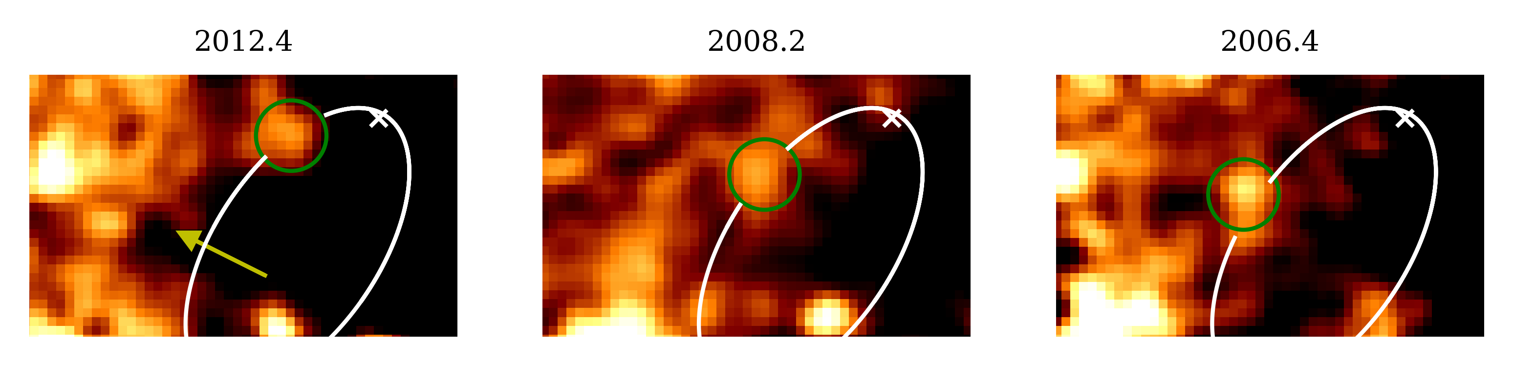
Figure 23: Disputed tail of the assumed cloud. This figure is inspired by Gillessen et al. (2013b) (see Fig. 9 in the related work). The yellow arrow marks the position of the possible tail emission. Sgr A* is located at the $\times$. The circle indicates the position of the G2/DSO. North is up, East is to the left. The size of every panel is $0.61"\,\times\,0.37"$.

In Fig. 23, we show the collapsed line maps where we adapt the settings given in Gillessen et al. (2013b). We select 25 channels between $2.1695\,\mu m\,-\,2.1815\,\mu m$. Furthermore, we subtract the averaged neighboring channels and smooth the resulting images with a 3 px Gaussian beam. Since the Br$\gamma$ emission, which is associated with the tail, can be found in 2006, 2008, and 2012, we conclude that the indicated feature in Gillessen et al. (2013b) is rather background related. We advice the reader to compare the orbit and the line emission position of the tail in Fig. 1 and Fig. 3 of Pfuhl et al. (2015). Please consider the mismatching emission of the tail and the position of the slit as presented in Fig. 10 and Fig. 12 in Plewa et al. (2017) that povides inconsistent information. While the tail seems to be on the same orbit as G2/DSO (Fig. 1 in Pfuhl et al., 2015; Gillessen et al., 2019), it is clearly misplaced as shown in the contour plot of Fig. 10 in Plewa et al. (2017).

Appendix D Brackett-$\gamma$ line-width as a function of time

Here we present a zoomed-in view of Figure 5 with about $15\%$ of the initial boundary range. As mentioned before, the black and orange line are related to the bow-shock model discussed in Zajaček et al. (2016). This bow-shock model shows a strong correlation to the observed line-width. Due to the OH lines Q1 and Q2 (see Table 3), the pollution of the line-width in 2015 is most probably higher than measured. Hence, the data point in 2015 is an upper limit. Averaging the two post-pericenter data point in 2014.6 and 2015.4 results in an line-width of $247.5\,km/s$ which is in agreement with the presented bow-shock model. The green dashed line in Fig. 25 agrees with the foreshortening factor discussed by Valencia-S. et al. (2015).

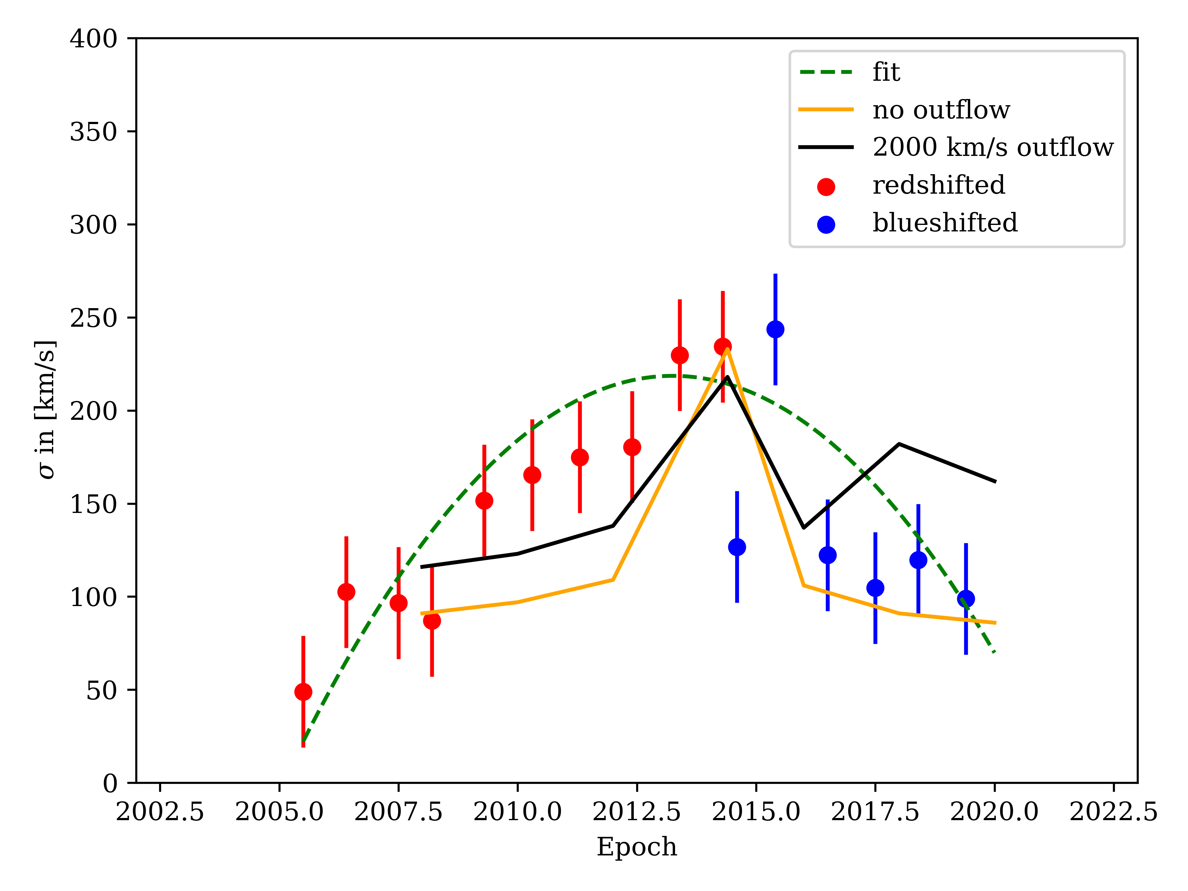
Figure 25: Zoomed-in view of Figure 5. We fit a second-degree polynomial function to the data (green dashed line). Based on accretion effects in combination of the foreshortening factor (see Sec. 4.5.1 for details), a variation of the line-width is expected. The prominent line-width that is related to a cloud-model (see Fig. 5) cannot be confirmed.

Appendix E Line of sight velocity of the OS sources

As for the G2/DSO, we use the Doppler-shifted Br$\gamma$ line to derive a LOS velocity v_z. The line evolution of OS1 and OS2 both are following a Keplerian approach (see Fig. 26 and Fig. 27). We use the same tools and techniques for the analysis of OS1 and OS2 as for the G2/DSO.

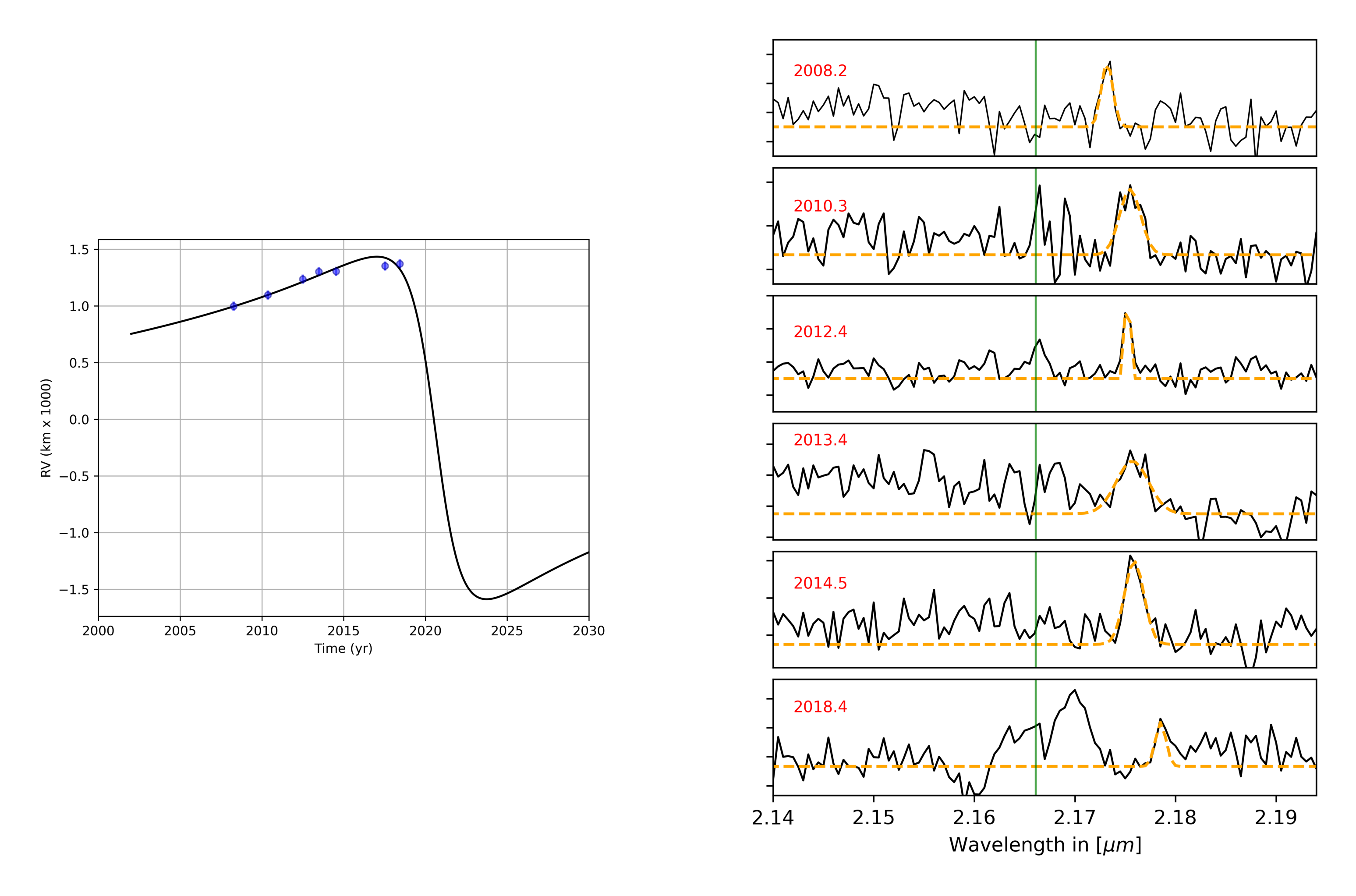
Figure 26: Evolution of the redshifted Br$\gamma$ line of OS1.

Figure 27: Evolution of the redshifted Br$\gamma$ line of OS2.

	OS1			OS2
Epoch	Wavelength	Velocity	Standard deviation $\sigma$	Wavelength	Velocity	Standard deviation $\sigma$ in [km/s]
	in [$\mu m$]	in [km/s]	in [km/s]	in [$\mu m$]	in [km/s]	in [km/s]
2007.5	-	-	-	2.1713	728.94	93.37
2008.2	2.1731	982.76	78.51	-	-	-
2010.3	2.1754	1300.48	145.25	2.1714	747.22	61.18
2012.4	2.1752	1266.56	17.93	2.1716	773.58	33.78
2013.4	2.1757	1332.03	223.71	2.1715	750.70	72.00
2014.5	2.1758	1356.56		2.1716	767.65	105.85
2015.4	-	-	-	2.1717	783.34	65.47
2017.5	-	-	-	2.1718	793.48	68.66
2018.4	2.1785	1721.30	72.12	2.1722	853.79	80.74

Table 14: Measured Doppler-shifted wavelengths and velocities for the OS sources. In some years, close-by or overlapping stellar sources hindered a confusion-free detection of the emission line. Epoch is given in decimal years.

Appendix F Positions of G2/DSO, OS1, and OS2

In this section, we list the used values for the Keplerian fit that are presented in this work for G2/DSO, OS1, and OS2. The fitted velocity information are listed in Table 4 and Table 14. We furthermore show the K-band continuum position of G2/DSO based on the high-pass filtered images presented in Fig. 10. We use a Gaussian to derive the K-band positions and combine them with the orbital solution (Table 5) of the source.

	G2/DSO				OS1				OS2
Epoch	Position in [mas]				Position in [mas]				Position in [mas]
	x	y	$\Delta$x	$\Delta$y	x	y	$\Delta$x	$\Delta$y	x	y	$\Delta$x	$\Delta$y
2005.5	-212.91	-116.55	5.61	2.23	-	-	-	-	-	-	-	-
2006.4	-205.05	-98.55	2.20	2.26	-	-	-	-	-	-	-	-
2007.5	-183.97	-87.08	4.59	4.69	-	-	-	-	-372.22	-188.87	3.56	3.62
2008.2	-170.58	-77.62	1.22	1.28	-313.43	-97.25	12.5	12.5	-388.52	-209.72	10.10	10.25
2009.3	-154.71	-69.36	2.41	2.10	-	-	-	-	-	-	-	-
2010.3	-141.01	-33.39	1.60	1.28	-304.86	-69.6	12.5	12.5	-399.42	-191.00	5.47	4.05
2011.3	-127.53	-28.15	1.59	1.74	-	-	-	-	-395.33	-196.80	4.43	9.96
2012.4	-101.59	-21.80	1.78	2.11	-240.65	-33.46	12.5	12.5	-387.88	-183.125	3.512	3.77
2013.4	-71.59	1.42	1.88	1.53	-205.47	-20.37	12.5	12.5	-377.67	-186.00	5.15	12.27
2014.3	-27.42	26.19	1.71	1.39	-	-	-	-	-	-	-	-
2014.5	44.52	-12.49	2.98	2.83	-189.51	-9.45	12.5	12.5	-351.13	-172.47	2.85	3.12
2015.4	51.87	-31.21	2.05	3.00	-	-	-	-	-348.02	-163.56	10.15	4.12
2016.5	41.30	-86.89	2.07	3.68	-	-	-	-	-323.35	-155.70	2.80	1.92
2017.5	37.48	-112.20	2.65	2.5	-177.72	-7.68	12.5	12.5	-331.28	-133.11	29.07	4.43
2018.4	39.13	-140.07	7.28	3.63	-110.58	12.91	12.5	12.5	-315.61	-134.58	3.05	3.85
2019.4	15.06	-161.88	1.62	2.07	-	-	-	-	-	-	-	-

Table 15: Positions of G2/DSO, OS1, and OS2. The values are in mas, the uncertainty is adapted from the Gaussian fit of the position. The epoch refers here to decimal years.

Appendix G MCMC results of the orbital elements of G2/DSO and the OS sources

Here we present the results of our MCMC simulations. As for the G2/DSO, the likelihood for the Keplerian fit is minimized. Hence, the MCMC simulations confirm our initial parameters to a satisfying degree (see Fig. 29, Fig. 30, and Fig. 31). The quality of the derived Keplerian parameters is underlined by the compactness of the possible randomized value distribution.

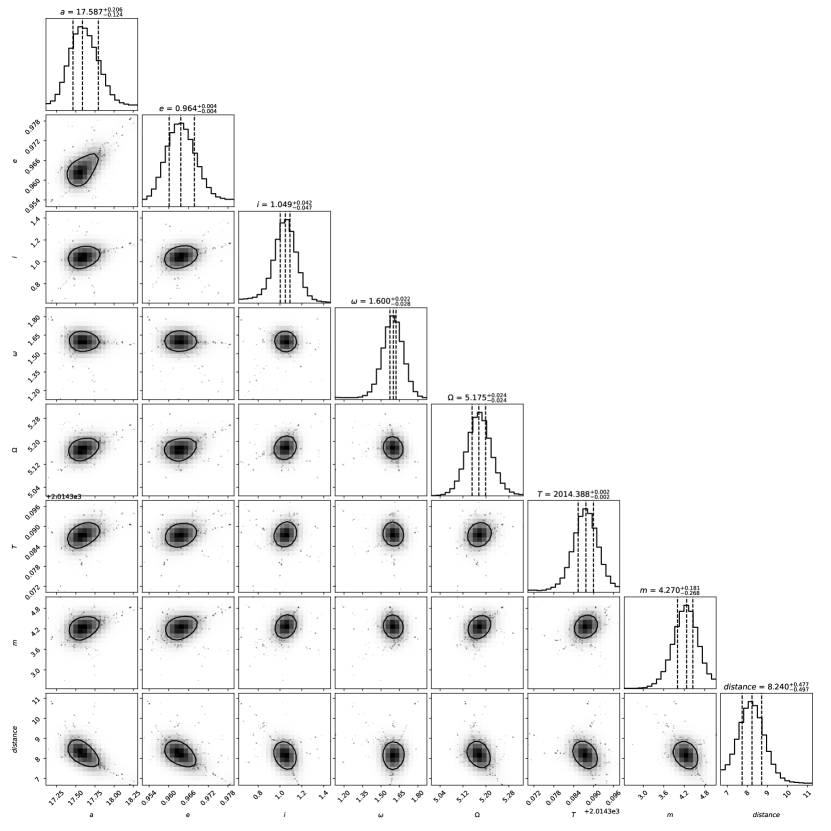
Figure 29: MCMC simulations of the Keplerian fit parameters of G2/DSO. The mean of the posterior distribution is in agreement with the input parameters which underlines the robustness of the Keplerian fit.

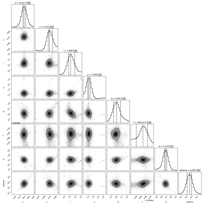
Figure 30: MCMC simulations for the orbital elements of OS1.

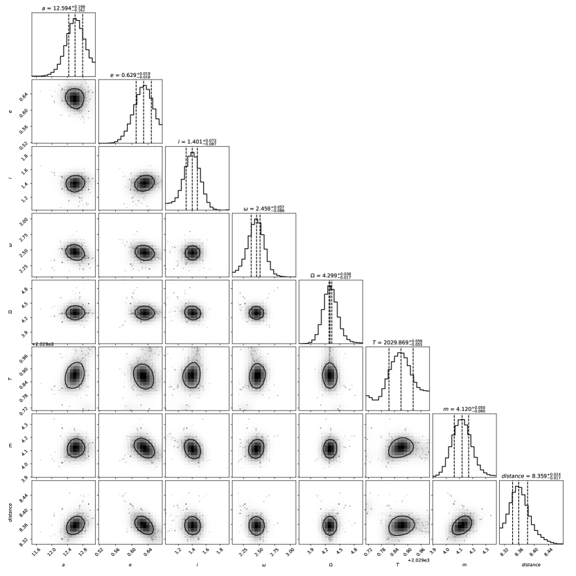
Figure 31: MCMC simulations for the orbital elements of OS1.

References

- Alexander (2017) Alexander, T. 2017, ARA&A, 55, 17, doi: 10.1146/annurev-astro-091916-055306
- Ali et al. (2020) Ali, B., Paul, D., Eckart, A., et al. 2020, ApJ, 896, 100, doi: 10.3847/1538-4357/ab93ae
- Ariew (1976) Ariew, R. 1976, Ockham’s Razor: A Historical and Philosophical Analysis of Ockham’s Principle of Parsimony (Champaign-Urbana: University of Illinois press)
- Bartko et al. (2009) Bartko, H., Martins, F., Fritz, T. K., et al. 2009, ApJ, 697, 1741, doi: 10.1088/0004-637X/697/2/1741
- Becerra-Vergara et al. (2020) Becerra-Vergara, E. A., Argüelles, C. R., Krut, A., Rueda, J. A., & Ruffini, R. 2020, A&A, 641, A34, doi: 10.1051/0004-6361/201935990
- Bonnet et al. (2004) Bonnet, H., Abuter, R., Baker, A., et al. 2004, The Messenger, 117, 17
- Bouchet et al. (2015) Bouchet, P., García-Marín, M., Lagage, P.-O., et al. 2015, Publications of the Astronomical Society of the Pacific, 127, 612, doi: 10.1086/682254
- Burkert et al. (2012) Burkert, A., Schartmann, M., Alig, C., et al. 2012, ApJ, 750, 58, doi: 10.1088/0004-637X/750/1/58
- Cheng et al. (2020) Cheng, Y., Andersen, M., & Tan, J. 2020, ApJ, 897, 51, doi: 10.3847/1538-4357/ab93bc
- Christopher et al. (2005) Christopher, M. H., Scoville, N. Z., Stolovy, S. R., & Yun, M. S. 2005, ApJ, 622, 346, doi: 10.1086/427911
- Ciurlo et al. (2020) Ciurlo, A., Campbell, R. D., Morris, M. R., et al. 2020, Nature, 577, 337, doi: 10.1038/s41586-019-1883-y
- Clénet et al. (2005) Clénet, Y., Rouan, D., Gratadour, D., Gendron, E., & Lacombe, F. 2005, in Science with Adaptive Optics, ed. W. Brandner & M. E. Kasper (Berlin, Heidelberg: Springer Berlin Heidelberg), 286–290
- Davies (2007) Davies, R. I. 2007, MNRAS, 375, 1099
- Dinh et al. (2021) Dinh, C. K., Salas, J. M., Morris, M. R., & Naoz, S. 2021, arXiv e-prints, arXiv:2102.09569. https://arxiv.org/abs/2102.09569
- Do et al. (2019a) Do, T., Hees, A., Ghez, A., et al. 2019a, Science, 365, 664, doi: 10.1126/science.aav8137
- Do et al. (2019b) Do, T., Witzel, G., Gautam, A. K., et al. 2019b, ApJ, 882, L27, doi: 10.3847/2041-8213/ab38c3
- Eckart et al. (2002) Eckart, A., Genzel, R., Ott, T., & Schödel, R. 2002, MNRAS, 331, 917, doi: 10.1046/j.1365-8711.2002.05237.x
- Eckart et al. (2004) Eckart, A., Moultaka, J., Viehmann, T., Straubmeier, C., & Mouawad, N. 2004, ApJ, 602, 760, doi: 10.1086/381178
- Eckart et al. (2013) Eckart, A., Mužić, K., Yazici, S., et al. 2013, aap, 551, A18, doi: 10.1051/0004-6361/201219994
- Eckart et al. (2017) Eckart, A., Hüttemann, A., Kiefer, C., et al. 2017, Foundations of Physics, 47, 553, doi: 10.1007/s10701-017-0079-2
- Eisenhauer et al. (2003) Eisenhauer, F., Abuter, R., Bickert, K., et al. 2003, in Proc. SPIE, Vol. 4841, Instrument Design and Performance for Optical/Infrared Ground-based Telescopes, ed. M. Iye & A. F. M. Moorwood, 1548–1561, doi: 10.1117/12.459468
- Fragione et al. (2017) Fragione, G., Capuzzo-Dolcetta, R., & Kroupa, P. 2017, MNRAS, 467, 451, doi: 10.1093/mnras/stx106
- Fragione & Loeb (2020) Fragione, G., & Loeb, A. 2020, ApJ, 901, L32, doi: 10.3847/2041-8213/abb9b4
- Ghez et al. (2003) Ghez, A. M., Duchêne, G., Matthews, K., et al. 2003, ApJ, 586, L127, doi: 10.1086/374804
- Gillessen et al. (2009) Gillessen, S., Eisenhauer, F., Trippe, S., et al. 2009, ApJ, 692, 1075, doi: 10.1088/0004-637X/692/2/1075
- Gillessen et al. (2012) Gillessen, S., Genzel, R., Fritz, T. K., et al. 2012, Nature, 481, 51, doi: 10.1038/nature10652
- Gillessen et al. (2013a) —. 2013a, ApJ, 774, 44, doi: 10.1088/0004-637X/774/1/44
- Gillessen et al. (2013b) —. 2013b, ApJ, 763, 78, doi: 10.1088/0004-637X/763/2/78
- Gillessen et al. (2017) Gillessen, S., Plewa, P. M., Eisenhauer, F., et al. 2017, ApJ, 837, 30, doi: 10.3847/1538-4357/aa5c41
- Gillessen et al. (2019) Gillessen, S., Plewa, P. M., Widmann, F., et al. 2019, ApJ, 871, 126, doi: 10.3847/1538-4357/aaf4f8
- Goicoechea et al. (2018) Goicoechea, J. R., Pety, J., Chapillon, E., et al. 2018, A&A, 618, A35, doi: 10.1051/0004-6361/201833558
- Gould & Quillen (2003) Gould, A., & Quillen, A. C. 2003, ApJ, 592, 935, doi: 10.1086/375840
- Gravity Collaboration et al. (2018) Gravity Collaboration, Abuter, R., Amorim, A., et al. 2018, A&A, 615, L15, doi: 10.1051/0004-6361/201833718
- Hills (1988) Hills, J. G. 1988, Nature, 331, 687, doi: 10.1038/331687a0
- Hobbs & Nayakshin (2009) Hobbs, A., & Nayakshin, S. 2009, MNRAS, 394, 191, doi: 10.1111/j.1365-2966.2008.14359.x
- Hopman & Alexander (2006) Hopman, C., & Alexander, T. 2006, ApJ, 645, 1152, doi: 10.1086/504400
- Hosseini et al. (2020) Hosseini, S. E., Zajaček, M., Eckart, A., Sabha, N. B., & Labadie, L. 2020, A&A, 644, A105, doi: 10.1051/0004-6361/202037724
- Hsieh et al. (2021) Hsieh, P.-Y., Koch, P. M., Kim, W.-T., et al. 2021, ApJ, 913, 94, doi: 10.3847/1538-4357/abf4cd
- Ishii et al. (1998) Ishii, M., Nagata, T., Sato, S., et al. 1998, AJ, 116, 868, doi: 10.1086/300467
- Jalali et al. (2014) Jalali, B., Pelupessy, F. I., Eckart, A., et al. 2014, MNRAS, 444, 1205, doi: 10.1093/mnras/stu1483
- Jia et al. (2019) Jia, S., Lu, J. R., Sakai, S., et al. 2019, ApJ, 873, 9, doi: 10.3847/1538-4357/ab01de
- Kohler (2017) Kohler, S. 2017, The Story of a Boring Encounter with a Black Hole, AAS Nova Highlights
- Kozai (1962) Kozai, Y. 1962, AJ, 67, 591, doi: 10.1086/108790
- Lada (1987) Lada, C. J. 1987, in IAU Symposium, Vol. 115, Star Forming Regions, ed. M. Peimbert & J. Jugaku, 1
- Lidov (1962) Lidov, M. L. 1962, Planet. Space Sci., 9, 719, doi: 10.1016/0032-0633(62)90129-0
- Löckmann et al. (2008) Löckmann, U., Baumgardt, H., & Kroupa, P. 2008, ApJ, 683, L151, doi: 10.1086/591734
- Lu et al. (2009) Lu, J. R., Ghez, A. M., Hornstein, S. D., et al. 2009, ApJ, 690, 1463, doi: 10.1088/0004-637X/690/2/1463
- Lucy (1974) Lucy, L. B. 1974, AJ, 79, 745, doi: 10.1086/111605
- Modigliani et al. (2007) Modigliani, A., Hummel, W., Abuter, R., et al. 2007, ArXiv Astrophysics e-prints
- Morris & Serabyn (1996) Morris, M., & Serabyn, E. 1996, ARA&A, 34, 645, doi: 10.1146/annurev.astro.34.1.645
- Moser et al. (2017) Moser, L., Sánchez-Monge, Á., Eckart, A., et al. 2017, A&A, 603, A68, doi: 10.1051/0004-6361/201628385
- Moultaka et al. (2015) Moultaka, J., Eckart, A., & Mužić, K. 2015, ApJ, 806, 202, doi: 10.1088/0004-637X/806/2/202
- Moultaka et al. (2005) Moultaka, J., Eckart, A., Schödel, R., Viehmann, T., & Najarro, F. 2005, A&A, 443, 163, doi: 10.1051/0004-6361:20052819
- Murray-Clay & Loeb (2012) Murray-Clay, R. A., & Loeb, A. 2012, Nature Communications, 3, 1049, doi: 10.1038/ncomms2044
- Mužić et al. (2008) Mužić, K., Schödel, R., Eckart, A., Meyer, L., & Zensus, A. 2008, A&A, 482, 173, doi: 10.1051/0004-6361:20078352
- Naoz (2016) Naoz, S. 2016, ARA&A, 54, 441, doi: 10.1146/annurev-astro-081915-023315
- Nayakshin (2005) Nayakshin, S. 2005, MNRAS, 359, 545, doi: 10.1111/j.1365-2966.2005.08913.x
- Nayakshin et al. (2007) Nayakshin, S., Cuadra, J., & Springel, V. 2007, MNRAS, 379, 21, doi: 10.1111/j.1365-2966.2007.11938.x
- Parsa et al. (2017) Parsa, M., Eckart, A., Shahzamanian, B., et al. 2017, ApJ, 845, 22, doi: 10.3847/1538-4357/aa7bf0
- Paumard et al. (2006) Paumard, T., Genzel, R., Martins, F., et al. 2006, The Astrophysical Journal, 643, 1011. http://stacks.iop.org/0004-637X/643/i=2/a=1011
- Peißker (2018) Peißker, F. 2018, PhD thesis, Universität zu Köln. https://kups.ub.uni-koeln.de/8510/
- Peißker et al. (2021b) Peißker, F., Eckart, A., & Ali, B. 2021b, The Astrophysical Journal, 918, 25, doi: 10.3847/1538-4357/ac0efc
- Peißker et al. (2020a) Peißker, F., Eckart, A., & Parsa, M. 2020a, ApJ, 889, 61, doi: 10.3847/1538-4357/ab5afd
- Peißker et al. (2020c) Peißker, F., Eckart, A., Sabha, N. B., Zajaček, M., & Bhat, H. 2020c, ApJ, 897, 28, doi: 10.3847/1538-4357/ab9826
- Peißker et al. (2020d) Peißker, F., Eckart, A., Zajaček, M., Ali, B., & Parsa, M. 2020d, The Astrophysical Journal, 899, 50, doi: 10.3847/1538-4357/ab9c1c
- Peißker et al. (2020b) Peißker, F., Hosseini, S. E., Zajaček, M., et al. 2020b, A&A, 634, A35, doi: 10.1051/0004-6361/201935953
- Peißker et al. (2019) Peißker, F., Zajaček, M., Eckart, A., et al. 2019, A&A, 624, A97, doi: 10.1051/0004-6361/201834947
- Peißker et al. (2021a) Peißker, F., Ali, B., Zajaček, M., et al. 2021a, ApJ, 909, 62, doi: 10.3847/1538-4357/abd9c6
- Perets et al. (2007) Perets, H. B., Hopman, C., & Alexander, T. 2007, ApJ, 656, 709, doi: 10.1086/510377
- Pfuhl et al. (2015) Pfuhl, O., Gillessen, S., Eisenhauer, F., et al. 2015, ApJ, 798, 111, doi: 10.1088/0004-637X/798/2/111
- Plewa et al. (2017) Plewa, P. M., Gillessen, S., Pfuhl, O., et al. 2017, ApJ, 840, 50, doi: 10.3847/1538-4357/aa6e00
- Prodan et al. (2015) Prodan, S., Antonini, F., & Perets, H. B. 2015, ApJ, 799, 118, doi: 10.1088/0004-637X/799/2/118
- Raghavan et al. (2010) Raghavan, D., McAlister, H. A., Henry, T. J., et al. 2010, ApJS, 190, 1, doi: 10.1088/0067-0049/190/1/1
- Ressler et al. (2015) Ressler, M. E., Sukhatme, K. G., Franklin, B. R., et al. 2015, Publications of the Astronomical Society of the Pacific, 127, 675, doi: 10.1086/682258
- Rieke et al. (2015) Rieke, G. H., Wright, G. S., Böker, T., et al. 2015, Publications of the Astronomical Society of the Pacific, 127, 584, doi: 10.1086/682252
- Rousselot et al. (2000) Rousselot, P., Lidman, C., Cuby, J. G., Moreels, G., & Monnet, G. 2000, A&A, 354, 1134
- Sabha et al. (2012) Sabha, N., Eckart, A., Merritt, D., et al. 2012, A&A, 545, A70, doi: 10.1051/0004-6361/201219203
- Salas et al. (2021) Salas, J. M., Morris, M. R., & Naoz, S. 2021, AJ, 161, 243, doi: 10.3847/1538-3881/abefd3
- Salas et al. (2020) Salas, J. M., Naoz, S., & Morris, M. R. 2020, arXiv e-prints, arXiv:2010.04170. https://arxiv.org/abs/2010.04170
- Schartmann et al. (2012) Schartmann, M., Burkert, A., Alig, C., et al. 2012, ApJ, 755, 155, doi: 10.1088/0004-637X/755/2/155
- Schödel et al. (2010) Schödel, R., Najarro, F., Muzic, K., & Eckart, A. 2010, A&A, 511, A18, doi: 10.1051/0004-6361/200913183
- Schödel et al. (2002) Schödel, R., Ott, T., Genzel, R., et al. 2002, Nature, 419, 694, doi: 10.1038/nature01121
- Scoville & Burkert (2013) Scoville, N., & Burkert, A. 2013, apj, 768, 108, doi: 10.1088/0004-637X/768/2/108
- Scoville et al. (1986) Scoville, N. Z., Sanders, D. B., & Clemens, D. P. 1986, ApJ, 310, L77, doi: 10.1086/184785
- Shahzamanian et al. (2017) Shahzamanian, B., Zajaček, M., Valencia-S., M., et al. 2017, in The Multi-Messenger Astrophysics of the Galactic Centre, ed. R. M. Crocker, S. N. Longmore, & G. V. Bicknell, Vol. 322, 233–234, doi: 10.1017/S1743921316011819
- Shahzamanian et al. (2016) Shahzamanian, B., Eckart, A., Zajaček, M., et al. 2016, A&A, 593, A131, doi: 10.1051/0004-6361/201628994
- Stephan et al. (2016) Stephan, A. P., Naoz, S., Ghez, A. M., et al. 2016, MNRAS, 460, 3494, doi: 10.1093/mnras/stw1220
- Stephan et al. (2019) —. 2019, ApJ, 878, 58, doi: 10.3847/1538-4357/ab1e4d
- Stock et al. (2020) Stock, C., Caratti o Garatti, A., McGinnis, P., et al. 2020, A&A, 643, A181, doi: 10.1051/0004-6361/202038897
- Suková et al. (2021) Suková, P., Zajaček, M., Witzany, V., & Karas, V. 2021, ApJ, 917, 43, doi: 10.3847/1538-4357/ac05c6
- Tan (2000) Tan, J. C. 2000, ApJ, 536, 173, doi: 10.1086/308905
- Tan & McKee (2004) Tan, J. C., & McKee, C. F. 2004, in Astronomical Society of the Pacific Conference Series, Vol. 322, The Formation and Evolution of Massive Young Star Clusters, ed. H. J. G. L. M. Lamers, L. J. Smith, & A. Nota, 263. https://arxiv.org/abs/astro-ph/0403498
- Tartėnas & Zubovas (2020) Tartėnas, M., & Zubovas, K. 2020, MNRAS, 492, 603, doi: 10.1093/mnras/stz3484
- Tokunaga & Vacca (2007) Tokunaga, A. T., & Vacca, W. D. 2007, in Astronomical Society of the Pacific Conference Series, Vol. 364, The Future of Photometric, Spectrophotometric and Polarimetric Standardization, ed. C. Sterken, 409
- Tress et al. (2020) Tress, R. G., Smith, R. J., Sormani, M. C., et al. 2020, MNRAS, 492, 2973, doi: 10.1093/mnras/stz3600
- Tsuboi et al. (2018) Tsuboi, M., Kitamura, Y., Uehara, K., et al. 2018, Publications of the Astronomical Society of Japan, 70, 85, doi: 10.1093/pasj/psy080
- Ulmer-Moll et al. (2019) Ulmer-Moll, S., Figueira, P., Neal, J. J., Santos, N. C., & Bonnefoy, M. 2019, A&A, 621, A79, doi: 10.1051/0004-6361/201833282
- Valencia-S. et al. (2015) Valencia-S., M., Eckart, A., Zajaček, M., et al. 2015, ApJ, 800, 125, doi: 10.1088/0004-637X/800/2/125
- Šubr & Karas (2005) Šubr, L., & Karas, V. 2005, A&A, 433, 405, doi: 10.1051/0004-6361:20042089
- Wardle & Yusef-Zadeh (2008) Wardle, M., & Yusef-Zadeh, F. 2008, ApJ, 683, L37, doi: 10.1086/591471
- Witzel et al. (2014) Witzel, G., Ghez, A. M., Morris, M. R., et al. 2014, ApJ, 796, L8, doi: 10.1088/2041-8205/796/1/L8
- Witzel et al. (2017) Witzel, G., Sitarski, B. N., Ghez, A. M., et al. 2017, ApJ, 847, 80, doi: 10.3847/1538-4357/aa80ea
- Yusef-Zadeh et al. (2013a) Yusef-Zadeh, F., Royster, M., Wardle, M., et al. 2013a, ApJ, 767, L32, doi: 10.1088/2041-8205/767/2/L32
- Yusef-Zadeh et al. (2013b) —. 2013b, ApJ, 767, L32, doi: 10.1088/2041-8205/767/2/L32
- Zajacek & Tursunov (2019) Zajacek, M., & Tursunov, A. 2019, The Observatory, 139, 231. https://arxiv.org/abs/1904.04654
- Zajaček et al. (2016) Zajaček, M., Eckart, A., Karas, V., et al. 2016, MNRAS, 455, 1257, doi: 10.1093/mnras/stv2357
- Zajaček et al. (2017) Zajaček, M., Britzen, S., Eckart, A., et al. 2017, A&A, 602, A121, doi: 10.1051/0004-6361/201730532
- Zajaček et al. (2020) Zajaček, M., Araudo, A., Karas, V., Czerny, B., & Eckart, A. 2020, ApJ, 903, 140, doi: 10.3847/1538-4357/abbd94
- Zajaček et al. (2014) Zajaček, M., Karas, V., & Eckart, A. 2014, A&A, 565, A17, doi: 10.1051/0004-6361/201322713