Methanol Mapping in Cold Cores: Testing Model Predictions

Abstract

Chemical models predict that in cold cores gas-phase methanol is expected to be abundant at the outer edge of the CO depletion zone, where CO is actively adsorbed. CO adsorption correlates with volume density in cold cores, and, in nearby molecular clouds, the catastrophic CO freeze-out happens at volume densities above 10⁴ cm^-3. The methanol production rate is maximized there and its freeze-out rate does not overcome its production rate, while the molecules are shielded from UV destruction by gas and dust. Thus, in cold cores, methanol abundance should generally correlate with visual extinction that depends both on volume and column density. In this work, we test the most basic model prediction that maximum methanol abundance is associated with a local $A_{V}\sim 4$ mag in dense cores and constrain the model parameters with the observational data. With the IRAM 30 m antenna, we mapped the CH₃OH (2–1) and (3–2) transitions toward seven dense cores in the L1495 filament in Taurus to measure the methanol abundance. We use the Herschel/SPIRE maps to estimate visual extinction, and the C¹⁸O(2–1) maps from Tafalla & Hacar (2015) to estimate CO depletion. We explored the observed and modeled correlations between the methanol abundances, CO depletion, and visual extinction varying the key model parameters. The modeling results show that hydrogen surface diffusion via tunneling is crucial to reproduce the observed methanol abundances, and the needed reactive desorption efficiency matches the one deduced from laboratory experiments.

1 Introduction

Methanol is a key precursor for many complex organic and pre-biotic molecules found in regions of star- and planet formation and thus it is very important for the growth of molecular complexity in the interstellar medium. It is observed at all stages of star formation, including the dense cold molecular gas within starless cores, characterized by temperatures of $T\simeq 10$ K, gas densities $n({\rm H_{2}})>10^{4}$ cm^-3, and subsonic turbulence (e.g., Benson & Myers, 1989; Bergin & Tafalla, 2007; Keto & Caselli, 2008). Geppert et al. (2006) showed that gas-phase synthesis cannot account for the observed amounts of methanol in the cold gas, that implies that chemical processes on interstellar dust grains must play the major role in the formation of this molecule. Indeed, the laboratory studies by Watanabe & Kouchi (2002) and Fuchs et al. (2009) confirmed that methanol can be formed efficiently during the hydrogenation of CO molecules on surfaces of interstellar dust analogs at temperatures of $\sim$10 K. Once formed, part of the solid methanol is delivered from cold grains to the gas phase where it is widely observed. The delivery mechanism is not well understood. In cold dark star-forming clouds, methanol is most likely delivered to the gas phase via the so-called reactive desorption mechanism (Garrod et al., 2007; Minissale et al., 2016; Chuang et al., 2018). During reactive desorption events, a fraction of the energy released in exothermic surface reactions is spent by the formed molecule to overcome the Van der Waals force which bind it to the surface; in this way, reactive desorption occurs. The efficiency of reactive desorption, i.e. the probability that a reaction product will be released to the gas, depends on a number of factors including the exothermicity of a reaction, the properties of the underlying surface etc. Existing studies report very different values of the efficiency of reactive desorption for species and surfaces, including methanol and other products of CO hydrogenation (see e.g., Garrod et al., 2007; Vasyunin & Herbst, 2013a; Minissale et al., 2016; Fredon et al., 2017; Vasyunin et al., 2017; Wakelam et al., 2017). Unlike water ice mantles, surfaces rich in CO and CH₃OH are needed to have efficient reactive desorption, as found by Minissale et al. (2016). Observations of cold dense cores show strong depletion of CO molecule from the gas phase (Willacy et al., 1998; Caselli et al., 1999; Crapsi et al., 2005; Pagani et al., 2007). CO molecules efficiently freeze-out on cold dust grains, thus making them efficient chemical reactors producing methanol and other products of hydrogenation of carbon monoxide. Given the dynamical quiescence and near-spherical geometry of pre-stellar cores, one can utilize them as natural laboratories to study the poorly known details of methanol formation and its link to carbon monoxide.

Methanol emission toward cold dense cores is observed in integrated intensity maps as ring-like structures (see, e. g., Tafalla et al., 2006; Bizzocchi et al., 2014; Punanova et al., 2018b; Harju et al., 2020; Spezzano et al., 2020) or a single peak toward the core center (Nagy et al., 2019) if the cores have not experienced substantial CO freeze-out, maybe because of their relative dynamical youth compared to other dense cores. Methanol distribution within the ring-like structures is often inhomogeneous (see e.g., Bizzocchi et al., 2014; Harju et al., 2020). Jiménez-Serra et al. (2016) showed that abundances of methanol and other complex organic molecules (COMs) in the L1544 pre-stellar core are higher in the core shell, that corresponds to $A_{V}\sim$ 7.5–8 mag (see also Vastel et al., 2014). The model, presented in Vasyunin et al. (2017), predicts that the maximal gas-phase abundance of the organic species is at $A_{V}\sim$ 8 mag. Scibelli & Shirley (2020) presented a methanol survey toward the L1495 filament and detected methanol down to the line-of-sight $A_{V}=3$ mag, with 70^′′ beam of the Arizona Radio Observatory ARO 12 m antenna. In this work, we first test the most basic model prediction that maximum methanol abundance is associated with $A_{V}\simeq 8$ mag on the line of sight in dense cores (i.e. a local $A_{V}$ within the core of $\sim$4 mag). Second, we attempt to put observational constraints on the parametrizations of reactive desorption used in chemical models of pre-stellar cores. The advantage of this study is the wealth of spatial data from high-resolution mapping of seven dense cores embedded within the same filament L1495. This allowed us to constrain model parameters on a multitude of data points, in contrast to a number of previous studies.

The targets of our study are the cold cores in the well studied filamentary structure L1495 in the Taurus molecular cloud (Lynds, 1962), which is a nearby (130–135 pc distant; Schlafly et al., 2014; Roccatagliata et al., 2020), quiescent low-mass star-forming region. The filament contains tens of dense cores (Marsh et al., 2014), and about fifty low-mass protostars in different evolutionary stages (Rebull et al., 2010). Hacar et al. (2013) and Seo et al. (2015) note that some parts of the filament are young (B211 and B216) and others (B213 and B7) are more evolved and actively star-forming, based on the amount of embedded protostars, their class and the level of gas turbulence. The dense cores embedded in the filament were detected in N₂H⁺ (Hacar et al., 2013), dust continuum emission (Marsh et al., 2014) and in ammonia (Seo et al., 2015). The dense cores show low gas temperature decreasing toward their centers (8–12 K; Seo et al., 2015), subthermal gas motions (Seo et al., 2015; Punanova et al., 2018a), coherent velocity structure, and slow rotation (Punanova et al., 2018a). The recent observations of the methanol lines at 96.7 GHz toward 31 starless cores detected by Seo et al. (2015) show weaker detections of methanol toward the more evolved regions, and the highest methanol gas abundance in the outskirts of dense gas in B211 (Scibelli & Shirley, 2020).

This paper presents maps of methanol lines at 2 and 3 mm toward seven dense cores in the L1495 filament to study the chemical connection between gas phase methanol, visual extinction and CO depletion in molecular clouds. We use the observational results to constrain free parameters of the chemical model by Vasyunin et al. (2017) and test the model predictions. In Section 2, we present the details of observations and data reduction. In Section 3, we present the results of methanol column density measurements, abundance estimations, CO depletion, molecular hydrogen and visual extinction estimations, and describe the chemical modeling. In Section 5 we discuss the results and correlations between methanol abundance and visual extinction and CO depletion, comparison with the chemical model results and constraining of the model parameters. The conclusions are given in Section 6.

2 Observations and Data Reduction

Table 1: The mapped cores. The numbers are given according to Hacar et al. (2013), H2013, and Seo et al. (2015), S2015. The given coordinates are the central positions of the maps. The only protostellar core is indicated with an asterisk (*). The region names are given according to Barnard (1927).

Core		$\alpha_{J2000}$	$\delta_{J2000}$	Region
H2013	S2015	(h m s)	(∘ ′ ′′)
1	12, 13, 14	04:17:42.347	28:07:30.88	B10
6	8, 9	04:18:06.379	28:05:34.87	B10
7	19	04:18:11.343	27:35:33.07	B211
10	22	04:19:36.768	27:15:32.00	B213
11*	23*	04:19:42.154	27:13:31.03	B213
16	33	04:21:20.595	27:00:13.63	B213
–	35	04:24:20.600	26:36:02.00	B216

Table 2: Methanol lines observed in this study.

Transition	Frequencya	$E_{\rm up}/k^{a}$	$A^{a}$	$n_{\rm crit}^{c}$	$F_{\rm eff}$	$B_{\rm eff}$	$\Delta v_{\rm res}$	rms in $T_{\rm mb}$	$T_{\rm sys}$
	(GHz)	(K)	($10^{-5}$ s-1)	(105 cm-3)			(km s-1)	(K)	(K)
(21,2–$1_{1,1}$)-$E_{2}$	96.739362	12.53b	0.2558	0.82	0.95	0.80	0.06	0.08–0.17	70–100
(20,2–$1_{0,1}$)-$A^{+}$	96.741375	6.96	0.3408	1.09	0.95	0.80	0.06	0.08–0.17	70–100
(31,3–$2_{1,2}$)-$E_{2}^{d}$	145.097370	19.51	1.0957	2.74	0.93	0.73	0.04	0.06–0.14	100–160
(30,3–$2_{0,2}$)-$A^{+}$	145.103152	13.93	1.2323	13.2	0.93	0.73	0.04	0.06–0.14	100–160
(20,2–$1_{0,1}$)-$E_{1}$	96.744550	20.08b	0.3407	1.09	0.95	0.80	0.06	0.08–0.17	70–100
(30,3–$2_{0,2}$)-$E_{1}$	145.093760	27.1	1.2314	103	0.93	0.73	0.04e	0.06–0.14	100–160

Notes. ^aThe methanol 3 mm and 2 mm frequencies, 3 mm energies and Einstein coefficients are taken from Bizzocchi et al. (2014) following Xu & Lovas (1997) and Lees & Baker (1968), also available at the Jet Propulsion Laboratory (JPL) database (Pickett et al., 1998). ^bEnergy relative to the ground 0_0,0, A rotational state. ^cThe critical densities are calculated for kinetic temperature of 10 K with an assumption of optically thin lines. ^dThe parameters for the 2 mm methanol lines are taken from the JPL database (frequencies and energies, Pickett et al., 1998) and Leiden Atomic and Molecular Database, LAMDA, (Einstein coefficients, Schöier et al., 2005). ^eThe 2 mm methanol lines for cores Hacar01, Hacar11, and Seo35 were observed with the Fast Fourier Transform Spectrometer FTS 50 backend with spectral resolution of 50 kHz or 0.10 km s^-1. The transitions with $E_{\rm up}/k>20$ K (below the horizontal line) were not detected in the majority of the cores and were not used in the analysis (see Sect. 3.2.2 for details).

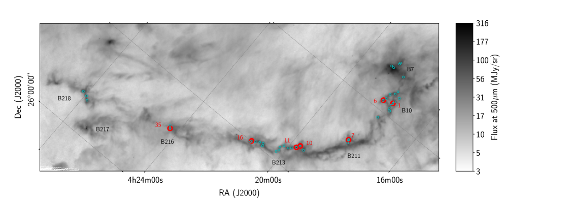
Figure 1: 500 $\mu$m dust continuum emission toward the L1495 filament of the Taurus molecular cloud mapped by Herschel/SPIRE (Palmeirim et al., 2013). The cyan circles show the 31 cores observed in methanol by Scibelli & Shirley (2020). Red numbered dots show the dense cores mapped in methanol in this work. We refer to the cores in this work according to these numbers (see Table 1).

We mapped six methanol lines at 96.7 GHz and 145.1 GHz toward seven dense cores of the L1495 filamentary structure (see Fig. 1 and Tables 1 and 2) with the IRAM 30 m telescope (IRAM projects 013-18, 125-18, and 031-19). The observations were performed on 2018 October 17–23, 2019 March 27–29 and September 16 under acceptable weather conditions, with precipitable water vapour $pwv$=1–10 mm. The on-the-fly maps were obtained with the Eight MIxer Receivers EMIR 090 (3 mm band) and EMIR 150 (2 mm band) heterodyne receivers in position switching mode, and the VESPA (VErsatile SPectrometer Assembly) backend. The spectral resolution was 20 kHz, the corresponding velocity resolutions were $\simeq$0.06 km s^-1 for the 3 mm band and $\simeq$0.04 km s^-1 for the 2 mm. The beam sizes were $\simeq$26^′′ for the 3 mm band and $\simeq$17^′′ for the 2 mm. The system temperatures were 90–627 K depending on the frequency.

The exact line frequencies, beam efficiencies, beam sizes, spectral resolutions and sensitivities are given in Table 2. Sky calibrations were obtained every 10–15 minutes. Reference positions were chosen individually for each core to make sure that the positions were free of any methanol emission. Pointing was checked by observing QSO B0316+413, QSO B0439+360, QSO B0605-085, Uranus, Mars or Venus every 2 hours and focus was checked by observing QSO B0439+360, Uranus, Mars or Venus every 6 hours.

The data reduction up to the stage of the convolved spectral data cubes was performed with the GILDAS/CLASS package. All data were convolved to the 26.8^′′ beam with the 8.7^′′ pixel, that is consistent with Nyquist sampling, for consistency of the data set. The following spectral analysis was performed with the Pyspeckit module of Python (Ginsburg & Mirocha, 2011).

Four out of six observed lines were detected with $S/N\!>\!5$ toward all seven cores. Two lines with the highest energy of the upper level ($E_{\rm up}\simeq 20$ K) were detected only toward the brightest areas of core 1. Therefore these two lines were not used for the analysis and only used to test our method of column density measurement (see Sect. 3.4 and Appendix A).

3 Results of observations

To test the model predictions, we apply the most widely used approaches to estimate $A_{V}$, CO depletion, and methanol abundance and use the most common data so our results would be easily compared to other works. We chose to use the Herschel dust continuum emission to measure the molecular hydrogen column density $N({\rm H_{2}})$ along with the conversion factor connecting $N({\rm H_{2}})$ and $A_{V}$, since the Herschel survey covered the majority of the selected molecular clouds. To measure the methanol column densities we chose the brightest 2 and 3 mm methanol lines. Based on the total nuclear spin of the hydrogen atoms in the methyl group, methanol can take $A$- and $E$-form. Once formed, $A$- and $E$-methanol molecules keep the hydrogen spines. The ratio of $A\!:\!E$ methanol depends on the temperature at which methanol was formed, with $A\!:\!E\!=\!1\!:\!1$ at 30–40 K, increasing at lower temperatures (see e.g., Wirström et al., 2011). At the temperatures of our cores, 10–12 K, the $A\!:\!E$ ratio should be $\simeq\!1.3$. In our observational set, we have only two lines of each methanol form, which is not enough to measure column densities via rotational diagrams robustly, so we combine them and assume the 1:1 $A\!:\!E$ methanol ratio. Besides that, Bizzocchi et al. (2014) found $A\!:\!E\!=\!1.03\!\pm\!0.26$ in another Taurus core, L1544. To measure the column densities of both methanol and CO we assumed the lines are consistent with local thermodynamic equilibrium (LTE) and optically thin emission (which is justified, see Sect. 3.2 and 3.4 for details). We also use a large homogeneous data set of typical dense cores in a low-mass star-forming region. To measure $T_{\rm dust}$ and $N({\rm H_{2}})$ we used the data from Herschel Spectral and Photometric Imaging Receiver, SPIRE, (Palmeirim et al., 2013). To trace CO depletion, we used the C¹⁸O(2–1) observations by Tafalla & Hacar (2015). We then used $N({\rm H_{2}})$ to measure the CO and methanol abundances. These steps are described in the following section.

3.1 H₂ column density and $A_{V}$

The Herschel space telescope carried out the most extensive coverage of dust continuum emission of the molecular clouds in our Galaxy, with PACS and SPIRE instruments. The Herschel science archive is the main source now for the dust continuum emission data in submillimeter range to estimate dust temperature and molecular hydrogen column densities in molecular clouds (see e.g., André et al., 2014; Friesen et al., 2017; Ladjelate et al., 2020).

We use the archive Herschel/SPIRE 250, 350, and 500 $\mu$m dust continuum emission map (Palmeirim et al., 2013) downloaded from the Herschel Science Archive (Observation ID 1342202254) to measure molecular hydrogen column density $N$(H₂), visual extinction $A_{V}$, and dust temperature $T_{\rm dust}$. We smooth the 250 and 350 $\mu$m maps to the largest beam (of 500 $\mu$m) of 38^′′ and fit a modified black body function. We use emissivity index $\beta=2.0$, typical for starless cores (Draine & Li, 2007; Schnee et al., 2010), close to the value $\beta=2.4$ previously found toward pre-stellar cores L1544 and Miz-2 in Taurus (Chacón-Tanarro et al., 2017; Bracco et al., 2017). We use dust opacity $\kappa_{250\mu m}$=0.144 cm² g^-1 based on $\kappa_{\nu}$=0.1($\nu$/10¹²[Hz])^β cm² g^-1 (Beckwith et al., 1990).

To measure visual extinction $A_{V}$, we scale H₂ column density following the conversion factor given in Güver & Özel (2009):

$$A_{V}=\frac{N{\rm(H_{2})[cm^{-2}]}}{1.105\times 10^{21}[{\rm cm^{-2}/mag}]}.$$ (1)

Our peak H₂ column density values agree within the errors or differ by 20% with those measured by Seo et al. (2015) using the 500 $\mu$m Herschel/SPIRE data only (see the comparison of the peak values in Table 3). To evaluate our H₂ column densities with an independent method, we scaled the $A_{V}$ map of L1495 by Schmalzl et al. (2010) to $N({\rm H_{2}})$ using the relation (1). In general, the column densities agree within 20% and differ by a factor of two in cores 11 and 35. The difference is not systematic (see the peak values in Table 3 and comparison of all available points in Fig. 12). The $A_{V}$ map by Schmalzl et al. (2010) was obtained by infrared photometric observations of background stars, so it suffers from gaps and interpolation effects, for example, there are two gaps covering a large area of core 35 and a gap toward core 11, those might have led to the factor of 2 difference in the estimated $N$(H₂). Thus we chose to use the Herschel data to measure both $N({\rm H_{2}})$ and $A_{V}$.

Table 3: Peak column and volume densities of H₂ toward the studied cores.

Core	$N({\rm H_{2}})$ (1022 cm-2)			$n({\rm H_{2}})$ (105 cm-3)
	SED	S10N	S15		*	S10n	M14	WT16
1	2.65	2.16	2.53${}^{+0.19}_{-0.07}$		1.50	–	26	0.69
6	2.57	3.21	2.64${}^{+0.17}_{-0.27}$		1.39	–	6.8	0.81
7	2.40	–	2.21${}^{+0.28}_{-0.28}$		0.78	–	1.9	0.40
10	2.07	2.26	1.71${}^{+0.15}_{-0.10}$		0.85	0.18	1.6	–
11	2.50	1.23	2.05${}^{+0.08}_{-0.07}$		1.83	0.18	–	–
16	2.80	2.80	2.38${}^{+0.21}_{-0.10}$		1.57	0.14	–	–
35	1.60	3.16	1.73${}^{+1.59}_{-0.36}$		0.51	0.17	–	–

Notes. Columns: SED – our $N({\rm H_{2}})$ based on modified black-body spectral energy distribution (SED); S10^N – $N({\rm H_{2}})$ based on conversion of $A_{V}$ from Schmalzl et al. (2010); S15 – $N({\rm H_{2}})$ from Seo et al. (2015); * – $n({\rm H_{2}})$ modeled in this work; S10ⁿ – $n({\rm H_{2}})$ from Schmalzl et al. (2010); M14 – $n({\rm H_{2}})$ from Marsh et al. (2014); WT16 – $n({\rm H_{2}})$ from Ward-Thompson et al. (2016).

3.2 CO depletion factor

In cold, dense, quiescent gas, CO freezes out onto dust grains and partly it is transformed into methanol. The level of CO freeze-out thus is one of the major factors affecting methanol formation (e.g., Whittet et al., 2011). It is commonly expressed as a CO depletion factor, $f_{d}$, that is defined as the ratio of the reference maximum abundance of CO ($X_{\rm ref}({\rm CO})$) in the cloud to the abundance of CO measured in the gas phase in the region of interest, $X$(CO). CO depletion is also often used as a chemical age indicator that helps to link the observed molecular abundances to the modeled ones (e.g., Jiménez-Serra et al., 2016; Lattanzi et al., 2020).

To measure the gas-phase CO abundance toward the cores, we use the C¹⁸O(2–1) maps obtained with the IRAM 30 m antenna, convolved to 23^′′ beam, by Tafalla & Hacar (2015), except for core 35 which belongs to the B216 region, there is no published C¹⁸O(2–1) map for B216. $X{\rm{}_{\rm ref}(CO)}$ is defined in Sect. 3.2.2.

3.2.1 C¹⁸O column densities

Tafalla & Hacar (2015) find more than one C¹⁸O line velocity components toward many positions in their map. Some of these components belong to the dense cores, the others belong to their envelopes or other material in the molecular cloud on the line of sight. Hacar et al. (2013) and Tafalla & Hacar (2015) resolve and analyze the material as small fibers composing the bigger filament. Since the molecular hydrogen column density measured both via $A_{V}$ and dust continuum emission do not contain kinematic information, we integrate all emission in the C¹⁸O(2–1) spectra to measure the integrated intensity $W$ and column density $N_{\rm tot}$.

To measure the C¹⁸O column densities, we assume that the C¹⁸O(2–1) lines are optically thin and consistent with LTE. Following Caselli et al. (2002), the column density then is:

$$N_{\rm tot}= \frac{8\pi W}{\lambda^{3}A_{ul}}\frac{g_{l}}{g_{u}}\frac{1}{J_{\nu}(T_{\rm ex})-J_{\nu}(T_{\rm bg})}\frac{1}{1-\exp{(-h\nu/kT_{\rm ex})}}$$ (2)

$$\times\frac{Q_{\rm rot}}{g_{l}\exp{(-E_{l}/kT_{\rm ex})}},$$

where $A_{ul}$ is the Einstein coefficient, $g_{l}$ and $g_{u}$ are the statistical weights of the upper and lower levels, $\lambda$ is the wavelength, $J_{\nu}(T)$ is the equivalent Rayleigh-Jeans temperature, $T_{\rm bg}$=2.7 K is the cosmic background temperature, $T_{\rm ex}$ is the excitation temperature, $E_{l}$ is the energy of the lower level. The partition function $Q_{\rm rot}$ of linear molecules (such as CO) is given by

$$Q_{\rm rot}=\sum_{J=0}^{\infty}(2J+1)\exp{(-E_{J}/kT)},$$ (3)

where $J$ is the rotational quantum number, $E_{J}=J(J+1)hB$, and $B$ is the rotational constant. We assume $T_{\rm ex}$=10 K which is consistent with the gas temperature measured by Seo et al. (2015). With $T_{\rm ex}$=10 K, equation 2 for the C¹⁸O(2–1) line can be simplified to $N_{\rm tot}\simeq$6.528$\times$10${}^{14}W$, where $W$ is in K km s^-1 and $N_{\rm tot}$ is in cm^-2.

The excitation conditions of C¹⁸O are close to those of the main isotopologue CO. The optically thin critical density of the C¹⁸O(2–1) transition is $2\times 10^{4}$ cm^-3, such that at lower densities it would deviate from LTE. With the statistical equilibrium radiative transfer code RADEX, we estimated that only toward the less dense outskirts of the cores ($n\sim 10^{3}$ cm^-3) $T_{\rm ex}\simeq 5$ K, which gives two times higher $N_{\rm tot}$ than that with LTE at 10 K.

3.2.2 CO depletion: choice of the reference CO abundance

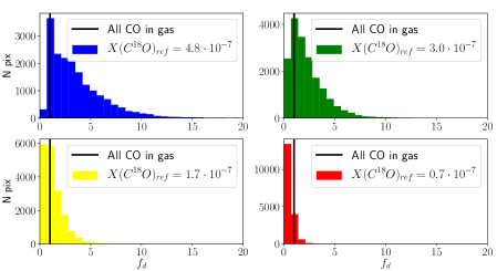
Figure 2: CO depletion $f_{d}$ measured across all B7, B10, B211, B213 and B218 regions, mapped by Tafalla & Hacar (2015), using various reference CO abundance. The black vertical line shows $f_{d}$=1, when all CO is in the gas phase.

The reference abundance of CO with respect to H₂ in the local interstellar medium (ISM) has been estimated in a number of studies with a spread between 0.4 and 2.7$\times 10^{-4}$ (Wannier, 1980; Frerking et al., 1982; Lacy et al., 1994; Tafalla & Santiago, 2004). The numbers given in literature are presented in Table 4.

Table 4: CO depletion with different $X{\rm(C^{18}O)}$.

$X$(CO)	$X{\rm(C^{18}O)}$	$f_{d}$			$N(f_{d}<1)$		citation	also used in
		min	median	max
0.39$\times$10-4*	$0.7\times 10^{-7}$	0.04	0.36	5.9	15954	70%	Tafalla & Santiago (2004)
0.85$\times$10-4	$1.7\times 10^{-7}$	0.09	0.87	14.4	8639	38%	Frerking et al. (1982)	Bacmann et al. (2002)
							Alonso-Albi et al. (2010)	Jørgensen et al. (2002)
								Crapsi et al. (2005)
1.7$\times$10-4	$3.0\times 10^{-7a}$	0.17	1.54	25.5	4675	20%	Lacy et al. (2017)
2.7${}^{+6.4}_{-1.2}\times 10^{-4}$	$4.8\times 10^{-7a}$	0.27	2.47	40.8	1625	7%	Lacy et al. (1994)	Lee et al. (2003)

^aAbundances found applying the fractional abundance ¹⁶O/¹⁸O=560 from Wilson & Rood (1994).

To choose the reference abundance of CO from the values given in Table 4, we calculated CO depletion factors for each data point of the entire C¹⁸O(2–1) map of L1495 filament provided in Tafalla & Hacar (2015) (B7, B10, B211, B213, B218). The area mapped by Tafalla & Hacar (2015) reaches the relatively diffuse outskirts of the filament, where CO should be undepleted. By definition, the depletion factor must be equal to unity there: $f_{d}=1$. Thus, our goal is to find the reference abundance of CO that provides the value of $f_{d}$ close to unity in the diffuse outskirts of the filament, and also ensures the minimum number of data points in the C¹⁸O(2–1) map of L1495 with nonphysical values of $f_{d}<1$. To estimate $f_{d}$, we use only well-defined column densities, with $N({\rm C^{18}O})/\Delta N({\rm C^{18}O})>5$. The resulting distributions of depletion factors across the entire L1495 map obtained for different reference abundances of CO are presented in Fig. 2. The chosen reference fractional abundances affect the CO depletion factor, with the highest $X_{\rm ref}$(CO) giving the largest $f_{d}$ and the widest range of $f_{d}$ (see Table 4). Taking into account the uncertainties of the calculated C¹⁸O column densities (including the LTE assumption, that results in underestimation of the column density), the first two reference abundances give median $f_{d}$ values in the cloud below 1, which is nonphysical. Toward the least depleted areas, we find $f_{d}\simeq 0.2$, 0.5, 0.9, and 1.5 with $X_{\rm ref}({\rm C^{18}O})=0.7\times 10^{-7}$, $1.7\times 10^{-7}$, $3.0\times 10^{-7}$, and $4.82\times 10^{-7}$, respectively. The choice of the reference value was based on the one which gave the lowest number of points (out of the total 22941) with $f_{d}<1$.

Thus we use the highest reference abundance of CO equal to 2.7$\times$10^-4 w.r.t. H₂ (which gives 4.8$\times$10^-7 of C¹⁸O w.r.t. H₂) that gives only 7% of nonphysical $f_{d}$ values across the maps, to measure CO depletion. These 7% may be caused by a large spread of this reference value (see Table 4 and Lacy et al., 1994). The number of the nonphysical values is small, and we do not aim at fitting the best reference CO abundance, we just use one of the well established reference values that fits better.

3.2.3 C¹⁸O abundance and CO-depletion factor

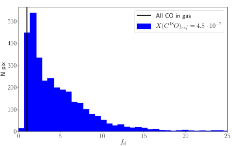
Figure 3: The distribution of CO depletion factor within the maps of all studied cores (except for core 35). The black vertical line represents $f_{d}$=1 (all CO in gas phase).

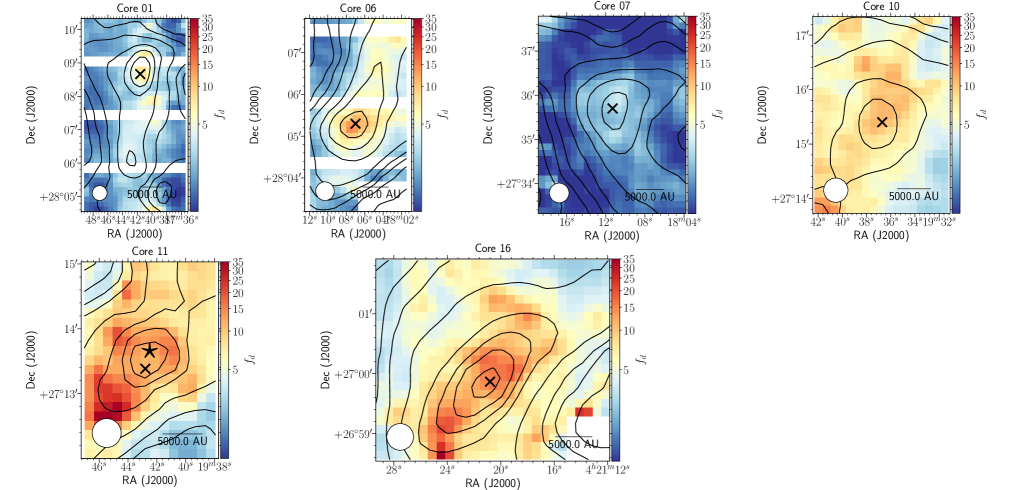
Figure 4: CO depletion factor (color scale) maps toward the observed cores based on C¹⁸O observations from Tafalla & Hacar (2015). Black contours show visual extinction at $A_{V}=$3, 4, 5, 6, 8, 12, 16, 20, 24 mag. The top $A_{V}$ contours are at $A_{V}$=24 mag for core 16 and at $A_{V}$=20 mag for the other cores. The black star shows the position of Class 0 protostar IRAS 04166+2706 (Santiago-García et al., 2009), crosses show the Herschel / SPIRE dust emission peaks. White circle on the bottom left of each map shows the 23^′′ beam. The white strips in the maps of cores 1 and 6 originate from the NaNs in the B10 map available at CDS.

The depletion factor of CO is generally moderate in L1495, ranging from 1 to 44 toward the studied cores (see Fig. 3 and 4; there are just a few pixels with high $f_{d}$, so we limit the histogram in Fig. 3 at $f_{d}$=25 to show the dynamic range better). Among them, core 7 shows the lowest depletion factor, $f_{d}$=1–4, as well as the entire B211 region with $f_{d}$=1–4. Cores 10, 11, and 16 (B213 region) show very similar depletion values, 2–44, the highest in our data set (that confirms B213 being more dynamically evolved than B211 and B10), with the median of $f_{d}$=6–8, high values both for starless and protostellar core. Cores 1 and 6 of the B10 region show intermediate values of $f_{d}$=1–14. Given the angular resolution of Herschel maps, these numbers could be lower limits of $f_{d}$. CO depletion toward core 35 was not measured since there are no available CO maps for this region.

3.3 Methanol distribution

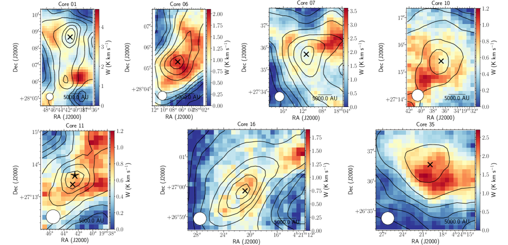
Figure 5: Integrated intensity of all observed methanol lines toward the observed cores (color scale) and visual extinction (black contours at $A_{V}=$3, 4, 5, 6, 8, 12, 16, 20, 24 mag). The top $A_{V}$ contours are at $A_{V}$=24 mag for core 16 and at $A_{V}$=20 mag for the other cores. Black star shows the position of Class 0 protostar IRAS 04166+2706 (Santiago-García et al., 2009), crosses show the Herschel / SPIRE dust emission peaks. White circle on the bottom left of each map shows the 26^′′ IRAM beam.

Figure 5 shows the distribution of integrated intensity over all observed methanol lines and contours of the dust continuum emission mapped with Herschel/SPIRE (Palmeirim et al., 2013) toward all seven observed cores. The gas phase methanol is expected to be most abundant in the areas where CO is actively freezing onto the dust grains, and the methanol production overcomes its freeze-out (see Vasyunin et al., 2017). We assume the lines are optically thin (see Sect. 3.4), so the methanol distribution can be traced by the intensity maps.

Toward three cores methanol appears in a shell around the densest area (cores 1, 7, and 10) where it is moderately (core 10) or significantly (cores 1 and 7) depleted. Toward two cores (6 and 16), methanol emission peaks are close to the dust emission peaks. Cores 11 and 35 show something in between: the methanol peaks are close to the dust emission peak, however the highest contour of methanol emission has an elongated arch-like shape and rather surrounds the highest dust emission contour. There are no CO observations for core 35.

The methanol emission in the methanol-rich shells around the cores 1, 7, 10, 11, and 35 is not uniform, with one or two spots of enhanced methanol toward each core. Such methanol distribution (in a shell around the dense parts with one or two emission peaks within the shell) was observed before toward other dense cores in Taurus (L1498, L1544, L1521E; Tafalla et al., 2006; Bizzocchi et al., 2014; Nagy et al., 2019) and Ophiuchus (Oph-H-MM1; Harju et al., 2020). We confirm that shell-like methanol distribution is also widespread in the dense cores of the L1495 filament.

3.4 Methanol column densities

We measure the methanol column densities via the rotational diagrams based on the four brightest lines detected across all cores. We use only the pixels with all four lines detected with signal-to-noise ratio $S/N\!>\!5$. We assume that the methanol lines are optically thin (as is shown in Scibelli & Shirley, 2020), consistent with LTE, and the fractional abundance of $A-$ and $E-$methanol is 1:1. We calculate the column density of the upper level population, $N_{\rm up}$, as

$$N_{\rm up}=\frac{8\pi kW\nu^{2}}{Ahc^{3}},$$ (4)

where $k$ is the Boltzmann constant, $W$ is the integrated intensity of the line, $\nu$ is the frequency, $A$ is the Einstein coefficient (given in Table 2), $h$ is the Planck constant, and $c$ is the speed of light (e.g., Goldsmith & Langer, 1999).

We fit a linear function $y=ax+b$ to the plot $\ln(N_{\rm up}/g_{\rm up})$ vs $E_{\rm up}/k$, where $g_{\rm up}$ is the statistical weight of the upper level ($g_{J}=2J+1$, with $J$ being the rotational quantum number), $E_{\rm up}$ is the energy of the upper level. Then the rotational temperature is $T_{\rm rot}=-1/a$, and the total column density is $N_{\rm tot}=e^{b}Q_{\rm rot}$, where $Q_{\rm rot}$ is the rotational partition function. For an asymmetric rotor (such as methanol) the partition function can be approximated as

$$Q_{\rm rot}=\frac{5.34\times 10^{6}}{\sigma}\sqrt{\frac{T_{\rm rot}^{3}}{ABC}},$$ (5)

where $\sigma=1$ is a symmetry number, $A$, $B$, and $C$ are the rotational constants (in MHz, taken from JPL; Pickett et al., 1998); for details see Gordy & Cook (1970). The uncertainty of the column density was calculated via propagation of errors of the $b$ coefficient. After measuring $T_{\rm rot}$ and $N_{\rm tot}$ we exclude all data points with relative uncertainties higher than 1/3 from our analysis.

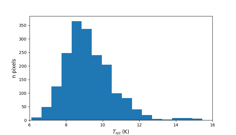
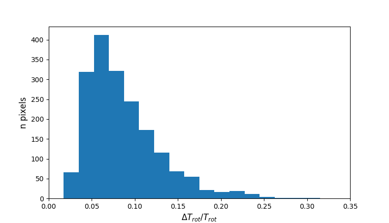
Figure 14: Distribution of $T_{\rm rot}$ based on the rotational diagrams (left) and the distribution of the relative uncertainties $\Delta T_{\rm rot}/T_{\rm rot}$ based on the rotational diagrams (right) of all available points with $S/N\!>\!5$ in the four lines used for the rotational diagrams.

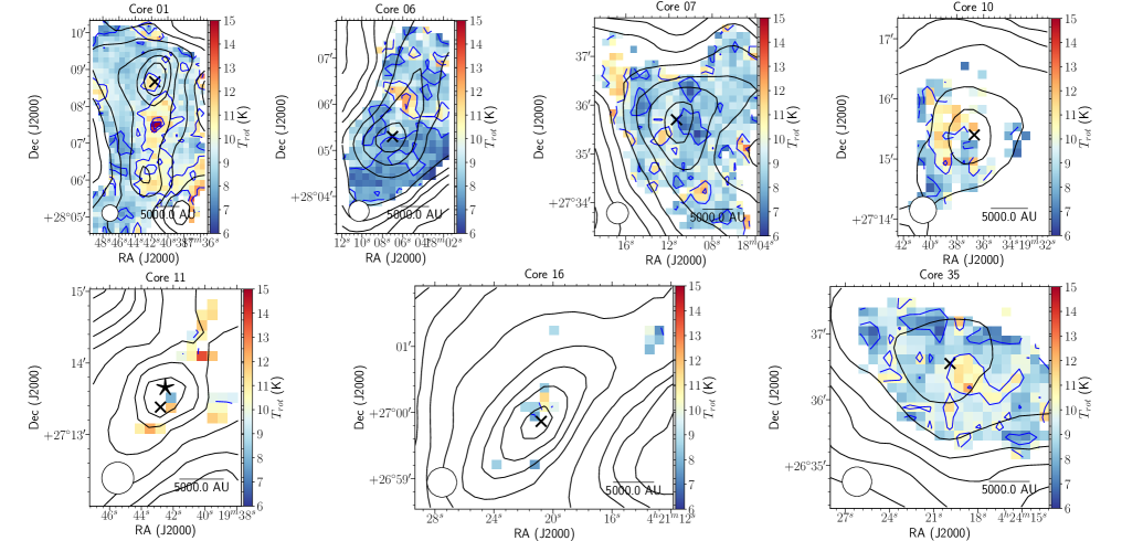
Figure 16: Rotational temperature line toward the observed cores (color scale and blue contours) and visual extinction (black contours at $A_{V}=$3, 4, 5, 6, 8, 12, 16, 20, 24 mag). The top $A_{V}$ contours are at $A_{V}$=24 mag for core 16 and at $A_{V}$=20 mag for the other cores. Black star shows the position of Class 0 protostar IRAS 04166+2706 (Santiago-García et al., 2009), crosses show the Herschel / SPIRE dust emission peaks. White circle on the bottom left of each map shows the 26^′′ IRAM beam.

The rotational temperature of methanol varies in the range of 6–16 K, with a typical uncertainty of 5–10% (see Fig. 14 for the $T_{\rm rot}$ and $\Delta T_{\rm rot}$ distributions and Fig. 16 for the $T_{\rm rot}$ maps). The median $T_{\rm rot}$=9.1 K is consistent with the gas temperatures of the cores (8–10 K) measured with ammonia by Seo et al. (2015), that also supports our assumption of LTE.

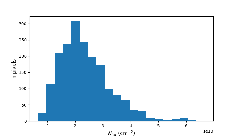
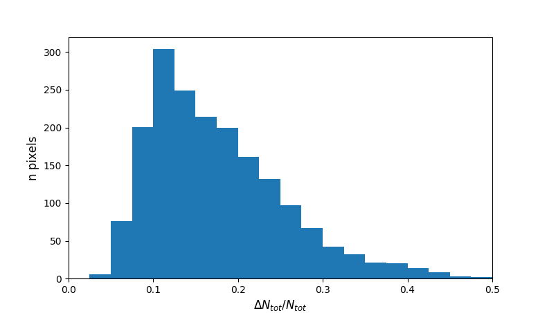
Figure 15: Distribution of $N_{\rm tot}$ based on the rotational diagrams (left) and the distribution of the relative uncertainties $\Delta N_{\rm tot}/N_{\rm tot}$ based on the rotational diagrams (right) of all available points with $S/N\!>\!5$ in the four lines used for the rotational diagrams.

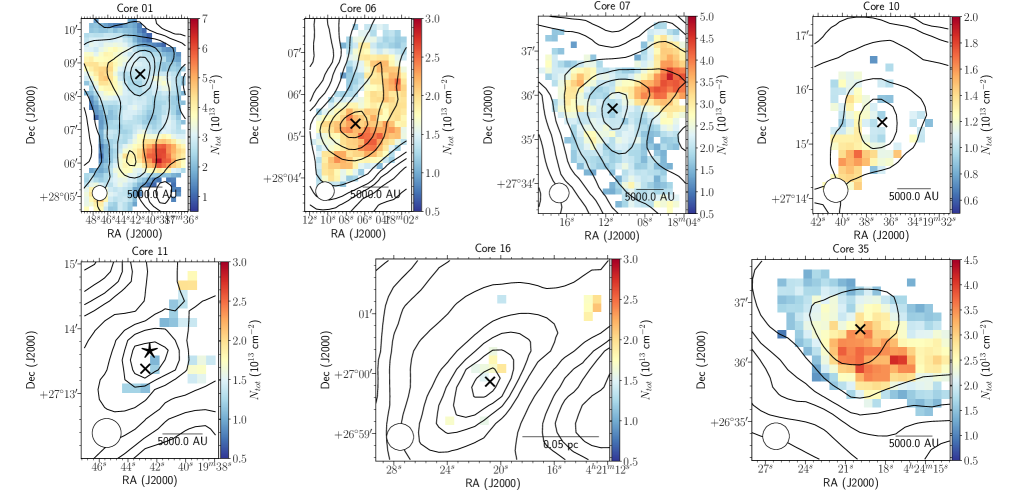
Figure 17: Methanol column densities toward the observed cores (color scale) and visual extinction (black contours at $A_{V}=$3, 4, 5, 6, 8, 12, 16, 20, 24 mag). The top $A_{V}$ contours are at $A_{V}$=24 mag for core 16 and at $A_{V}$=20 mag for the other cores. Black star shows the position of Class 0 protostar IRAS 04166+2706 (Santiago-García et al., 2009), crosses show the Herschel / SPIRE dust emission peaks. White circle on the bottom left of each map shows the 26^′′ IRAM beam.

The total methanol column density varies in the range of (0.5–7.0)$\times$10¹³ cm^-2 across all cores with typical uncertainty of 10–20% (see Fig. 15). Our column densities measured with the rotational diagrams are consistent with those measured with RADEX by Scibelli & Shirley (2020) toward the ammonia peaks. Figure 17 shows the column density maps. Since the brightest methanol emission avoids the dense core centers, we register higher column density values (up to 7$\times$10¹³ cm^-2) than Scibelli & Shirley (2020) did (up to 3.5$\times$10¹³ cm^-2), as they pointed only toward the ammonia peaks.

Since we assume the lines are optically thin, the column density distribution is similar to the distribution of the integrated intensity (see Fig. 17, although toward cores 11 and 16 we have only few points detected with $S/N\!>\!5$ in all four lines).

3.5 Methanol abundance

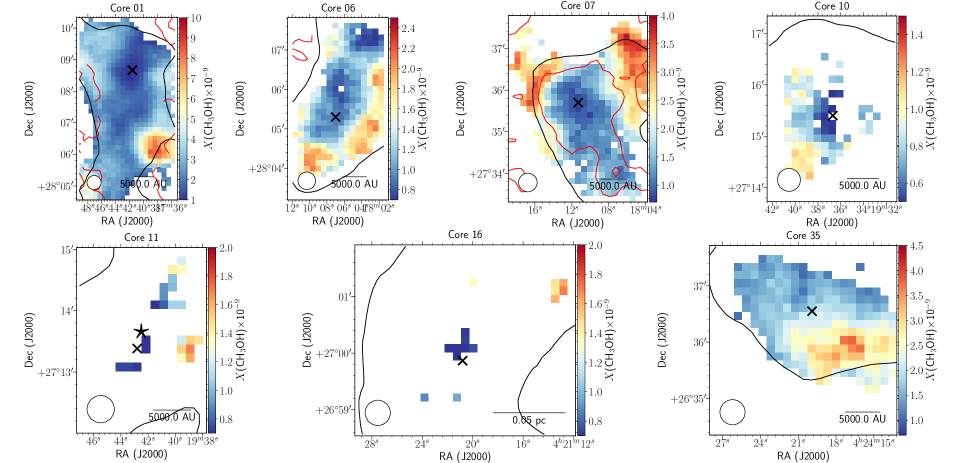
Figure 6: Methanol abundance maps. The red contours show $f_{d}$=1.6, the black contours show $A_{V}$=6 mag, the values of observed CO depletion and visual extinction, associated with the highest methanol abundance.

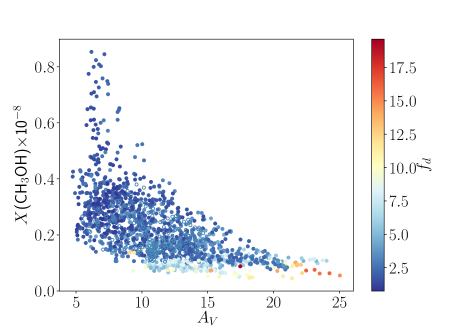
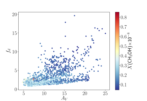
Figure 7: Left: the observed abundance of CH₃OH for all of the pixels in all of the maps combined as a function of line-of-sight visual extinction; the color scale represents the CO depletion factor. Right: the CO depletion factor as a function of line-of-sight visual extinction; the color scale represents the methanol abundance.

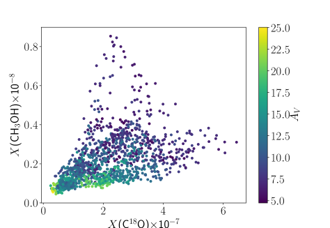
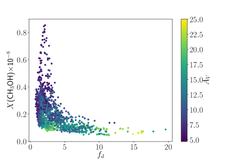
Figure 8: The observed abundance of CH₃OH for all of the pixels in all of the maps combined as a function of observed abundance of C¹⁸O (left) and CO-depletion factor (right). The color scale represents the line-of-sight visual extinction.

We use the $N$(H₂) obtained by fitting spectral energy distribution (SED) to the Herschel data to measure the methanol abundance. Methanol abundance maps are shown in Fig. 6. We obtain the methanol abundances of (0.5–8.5)$\times 10^{-9}$ with a median value of 1.9$\times 10^{-9}$ (see median column densities, rotational temperature and abundance of methanol toward individual cores in Table 5). Cores 1, 6, 7, 35, which belong to the less evolved regions B10, B211, and B216, show higher methanol abundance than cores 10, 11, 16 from the more evolved B213 region, by a factor of two. The highest methanol abundance (8.5$\times 10^{-9}$) is observed toward a local methanol peak in a shell around core 1. In all cores, the highest methanol abundance is observed in the shells around the cores, with $A_{V}\!=\!5-10$ mag (see the left panel of Fig. 7) and $f_{d}=1.5-2.0$ (see the right panel of Fig. 8), and correlates with gaseous CO abundance (see the left panel of Fig. 8). CO depletion factor increases with visual extinction (see the right panel of Fig. 7), however there is rather a general trend than a single correlation: $f_{d}$ always increases with $A_{V}$ within one core (see the plots of individual cores in Fig. 11). Sometimes the emission has a prominent peak of enhanced abundance (cores 1 and 35), on average associated with $A_{V}\simeq 6$ mag and $f_{d}\simeq 1.6$, which is well illustrated by the abundance maps of cores 1 and 7 in Fig. 6. For cores 10, 11, and 16 we do not have enough data points to test if the average rule applies to them. In all cores methanol is significantly depleted toward the dust peaks where the observed abundance is minimal (except for core 35 where minimal abundance is observed to the north of the dust peak).

In L1544 and Oph-H-MM1 the lopsided distribution of methanol in the shell was explained by the UV irradiation of one side and shielding of the other side of the cores (Spezzano et al., 2016; Harju et al., 2020) and the probable presence of a slow shock (Punanova et al., 2018b; Harju et al., 2020). In L1495, there are no preferred UV irradiation directions or areas shielded more than others (the background column density on either sides of the filament differs by a factor of 2; Palmeirim et al., 2013). Although locally illumination of the cores could be non-uniform: there are protostars of various classes in and around the filament. Besides that, from Hacar et al. (2013) we know that the cores reside in the dense “fertile” fibers next to less dense “sterile” fibers, those overlap along the line of sight and probably both shield methanol from UV destruction and contribute to the observed methanol abundance producing local abundance peaks like the ones toward cores 1 and 35. Yet there are no evidence of slow shocks in the L1495 cores: the local velocity gradients of the shells traced by the HCO⁺ emission show homogeneous patterns (Punanova et al., 2018a), except for the protostellar core 11.

4 Modeling chemical composition of the filament cores

4.1 Physical models of the cores

For the purpose of modeling, we assumed that the cores are spherically symmetric. Under this assumption, we derived temperature and density profiles of the cores. First, we used simple polynomial fits to the radial distributions of Herschel molecular column density ($N({\rm H_{2}})$). Then, we converted the molecular hydrogen column density to volume density. A similar approach was recently published in Hasenberger & Alves (2020). Two key assumptions in the performed procedure are (i) the cores are spherical and (ii) the cores can be divided into constant gas density “onion shells” of same thickness. We also assume that the model center coincides with the observed dust peak. The derived H₂ volume densities have been tested to provide the original H₂ column densities when using the reverse procedure of obtaining column densities from volume densities described in Jiménez-Serra et al. (2016). The physical models of the cores are shown in Fig. 9. Gas temperature in the cores was assumed equal to the dust temperature derived from Herschel data. This assumption is reasonable for our study, as we are focused on chemistry. The majority of chemical processes in the gas phase exhibit weak dependence on gas temperature. For example, rates of ion-molecule reactions that are believed to dominate low-temperature gas-phase chemistry, depend on temperature as $\sqrt{T_{\rm gas}}$. On the contrary, rates of chemical processes on surfaces of interstellar grains such as thermal desorption or thermal hopping of adsorbed species typically show exponential dependence on temperature. Moreover, at gas densities above 10⁴ cm^-3 gas and dust are close to thermal coupling (Goldsmith, 2001). Finally, the L1495 filament does not possess signs of violent processes such as shock waves that may heat the gas to very high temperatures (e.g., Tafalla & Hacar, 2015). Thus, we believe that our assumption on equality of gas and dust temperatures is justified.

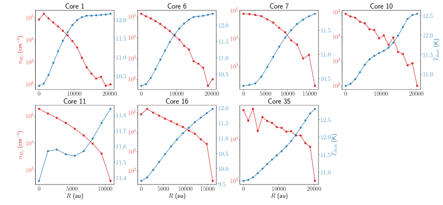
Figure 9: Physical models of the cores: molecular hydrogen number density (red) and dust temperature (blue).

4.2 Chemical model

Table 5: Median column densities, rotational temperatures and abundances of methanol for each core; the cores chemical ages, derived from the chemical model. The age estimates are based on the highest observed CO depletion factors.

Core	$N$(CH3OH)	$T_{\rm rot}$	$X$(CH3OH)	$f_{d}$	age
	(1013 cm-2)	(K)	$\times$10-9		(kyr)
1	2.81	9.3	2.68	8	118
6	1.83	8.2	1.28	14	226
7	2.23	8.9	1.76	4	89
10	1.18	9.0	0.84	12	433
11	1.39	10.9	1.07	44	1000
16	1.70	8.6	0.88	17	248
35	2.24	9.2	1.89	4a	187

Notes. ^aWe have no CO data for core 35, so we adapt the lowest $f_{d}$ observed toward our cores ($f_{d}$=4 for core 7), since the region B216 is supposed to be young (Hacar et al., 2013; Seo et al., 2015).

In this work, we utilize the MONACO chemical model previously described in Vasyunin et al. (2017) with several minor updates described in Nagy et al. (2019); Scibelli et al. (2021). This is a “three-phase” chemical model capable of simulating chemical evolution in the gas phase, on surfaces of icy mantles of interstellar dust grains, and in the bulk of icy mantles. MONACO is a 0D rate equations-based time-dependent chemical model. In order to simulate chemistry in pre-stellar cores, the chemical code is wrapped into a 1D static physical models that includes radial distributions of the most important physical parameters which control chemistry in a pre-stellar core: gas density, gas and dust temperatures, and visual extinction (see Sect. 4.1). With the model, time-dependent fractional abundances calculated with the MONACO code at each radial point of the 1D model, can be converted to column densities of species, thus allowing direct comparison with observational data.

Since dense cores considered in this work are located in a filament of molecular gas, we use a two-step approach to model their chemical evolution. On the first step, chemistry in a low-density translucent medium is simulated ($n_{\rm H}$ = 10² cm^-3, $T_{\rm gas}$ = $T_{\rm dust}$ = 20 K, $A_{V}$ = 2 mag) over a period of 10⁶ years. The initial chemical composition of the medium corresponds to elemental abundances 1 (EA1) from Table 1 in Wakelam & Herbst (2008). On the second step, chemical evolution in the core is simulated using the abundances of chemical species at the final moment of time of step one as initial chemical composition.

Other key parameters of the chemical model are the following. The cosmic-ray ionization rate is taken equal to the standard value of 1.3$\times$10^-17 s^-1. The dust grain radius in the model is 10^-5 cm. Four upper layers of multilayered grain mantle are considered as belonging to surface in accordance with Vasyunin & Herbst (2013b). The sticking probability for all species is unity (e.g., Fraser & van Dishoeck, 2004; Chaabouni et al., 2012, and references therein). Surface species can be delivered to the gas phase via thermal desorption, photodesorption, cosmic ray-induced desorption (Hasegawa & Herbst, 1993) and reactive desorption (RD).

Photodesorption yield for CO was measured in a number of laboratory experiments. It was found to be high, temperature- and wavelength-dependent, of the order of 10^-3–10^-1 molecules per incident photon (e.g., Öberg et al., 2009; Fayolle et al., 2011; Chen et al., 2014; Muñoz Caro et al., 2016; Paardekooper et al., 2016). We tested various CO photodesorption yields (0.001–0.1) applied to our four models and found that high CO photodesorption yield, 0.03 molecules per incident photon and higher, significantly affects process of CO depletion in the models of pre-stellar cores considered in this study. For two cores, observed CO depletion factors either never reached (core 11), or reached on timescales $>$10⁶ years (core 10). Such timescale is much longer than typical estimates of “chemical age” of pre-stellar cores, which is very uncertain, but in most studies is well below $10^{6}$ years: 1–3$\times\!10^{5}$ (e.g., Tafalla & Santiago, 2004; Walsh et al., 2009; Jiménez-Serra et al., 2016; Nagy et al., 2019; Lattanzi et al., 2020; Scibelli et al., 2021; Jiménez-Serra et al., 2021), sometimes up to 3–7$\times\!10^{5}$ years (e.g., Loison et al., 2020). Thus, with certain simplification, in this study we employed constant photodesorption yield for CO equal to 10^-2 molecules per incident photon, following Fayolle et al. (2011), where this value was obtained for UV field in pre-stellar cores in accurate experiments with tunable synchrotron radiation. For methanol, following Bertin et al. (2016) and Cruz-Diaz et al. (2016), we employed photodesorption yield equal to 10^-5 molecules per incident photon. This yield was also assumed for other species in the model.

The efficiency of reactive desorption, i.e., the probability of a product of an exothermic surface reaction to be ejected to the gas phase upon formation depends on the particular reaction, product and type of surface in a complex and still poorly studied (see e.g., Garrod et al., 2007; Vasyunin & Herbst, 2013a; Minissale et al., 2016; Chuang et al., 2018). Next, the rate of reactive desorption depends on the rate of related surface reaction. Rates of surface diffusive reactions of hydrogenation are mainly controlled by diffusion of atomic hydrogen. The rates of diffusion, in turn, are poorly known. Reactive desorption is believed to be the key process that delivers methanol, formed on cold grains during CO hydrogenation, to the gas phase (Garrod et al., 2006). Given that there are no known efficient gas-phase routes of methanol formation (Geppert et al., 2006), it is tempting to utilize the extensive observational data set on CO and CH₃OH presented in this study, to constrain model parameters related to the formation and desorption of methanol in the conditions of cold dense cores. Thus, we consider four parametrizations of reactive desorption and surface mobility of hydrogen atoms: (i) tunneling for hydrogen diffusion enabled, treatment of reactive desorption following Minissale et al. (2016) with parameters as in Vasyunin et al. (2017) (rdMD); (ii) no tunneling for hydrogen diffusion, only thermal hopping, diffusion/desorption energy ratio is 0.5, rdMD; (iii) tunneling for hydrogen diffusion, single reactive desorption probability of 1% (rd1); (iv) no tunneling for hydrogen diffusion, rd1. Those four particular models were chosen based on the fact that efficiency of quantum tunneling for atomic diffusion on grains is still debated (e.g., Rimola et al., 2014; Lamberts & Kästner, 2017). As of parametrizations of reactive desorption, we aim to check the feasibility of approaches utilized in our previous works (e.g., Vasyunin & Herbst, 2013a; Vasyunin et al., 2017), as well in a number of other studies (e.g., Garrod et al., 2007; Ruaud et al., 2016; Jin & Garrod, 2020).

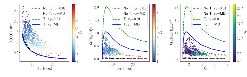
Figure 10: The comparison of the observed (colored dots) and modeled CO abundance profiles as a function of visual extinction (left); CH₃OH abundance profiles as a function of visual extinction (middle); and CO depletion factor (right) for core 1. The color scale represents CO depletion factor $f_{d}$ (left and middle) and visual extinction $A_{V}$ (right) in the individual pixels. The models include: no tunneling for diffusion of H and H₂ and 1% reactive desorption efficiency (dotted magenta line); no tunneling and reactive desorption efficiency from Minissale et al. (2016) (dashed-dotted black line); tunneling and 1% reactive desorption efficiency (dashed green line); tunneling and reactive desorption efficiency from Minissale et al. (2016) (solid blue line).

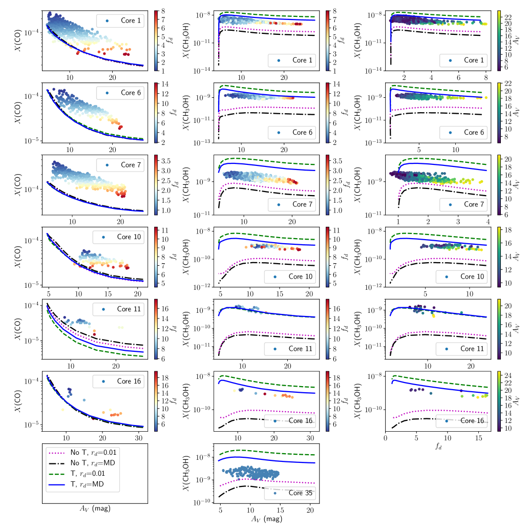
Figure 11: The comparison of the observed (colored dots) and modeled CO abundance profiles as a function of visual extinction (left); CH₃OH abundance profiles as a function of visual extinction (middle); and CO depletion factor (right) for all cores. The color scale represents CO depletion factor $f_{d}$ (left and middle) and visual extinction $A_{V}$ (right) in the individual pixels. The data points of core 35 are shown with plane color since there are no CO data for this core. The models include: no tunneling for diffusion of H and H₂ and 1% reactive desorption efficiency (dotted magenta line); no tunneling and reactive desorption efficiency from Minissale et al. (2016) (dashed-dotted black line); tunneling and 1% reactive desorption efficiency (dashed green line); tunneling and reactive desorption efficiency from Minissale et al. (2016) (solid blue line).

4.3 Observed and modeled abundances

Using the parameters described above, we performed 1D chemical modeling of all dense cores in the L1495 filament considered in this study. To estimate the chemical age of the cores, we used the highest depletion factor values reached in each core (see Table 5). Modeled radial profiles of CO and CH₃OH column densities and fractional abundances were then compared with the observed values. The four models produce almost the same CO abundance (see left panel of Fig. 10), while methanol abundance differ significantly from model to model (see central and right panels of Fig. 10). Although none of the models matches the observations perfectly, the model with quantum tunneling for diffusion of atomic hydrogen and treatment of reactive desorption according to parametrization by Minissale et al. (2016) produces results with the closest agreement to the observed data, as shown in Fig. 10 with an example of core 1. The left panels of Fig. 11 show the comparison of the observed CO abundances vs. visual extinction and the results of all four chemical models.

The best model reproduces the observed CO abundances very well with a slight (by a factor of a few) underestimation likely due to the fact that we see the CO emission from the cloud surrounding the cores. The other models (with higher reactive desorption and no tunneling) produce the same amount of CO (see left panel of Fig. 10 and 11). This result shows that the cores are close to spherical shape, and our assumption used to convert gas column density to volume density is applicable for our cores.

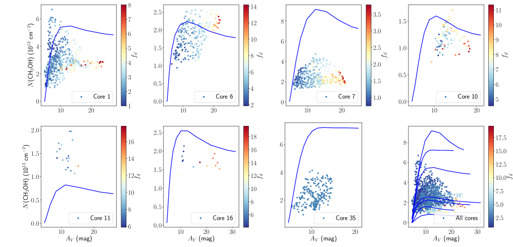
Figure 18: The comparison of the observed (colored dots) and modeled (solid blue line) CH₃OH column density profiles as a function of visual extinction. The color scale represents CO depletion factor $f_{d}$. The model includes tunneling for diffusion of H and H₂, and reactive desorption efficiency from Minissale et al. (2016).

In the middle panels of Fig. 11, observed and modeled abundances of methanol are presented. One can see that CH₃OH abundances obtained with the best fit model are overestimated by a factor of a few in all cores, similar to what was seen before in the models (like in L1521E in Scibelli et al., 2021), except core 11. In that core, the model matches the observed values well. However, the number of data points for core 11 is small. Another reason for the mismatch might be our assumption of the $A$:$E$ methanol ratio of 1:1. If we treat the two forms separately as is shown in Sect. 3.4, $E$-methanol shows higher column densities than $A-$, although with large uncertainties. On the other hand, Harju et al. (2020) present the ratio $A$:$E$=1.3. The complex correlation between methanol abundance and visual extinction is clearly seen both in the model and observations, as illustrated in Fig. 18: we detect the lowest methanol column densities at the outskirts of the cores, they rapidly increase with $A_{V}$ up to the line-of-sight $A_{V}\sim 8$, and then decrease with $A_{V}$.

In the right panels of Fig. 11, abundances of methanol vs. depletion factor $f_{d}$ are presented. Interestingly, the maximum abundances of CH₃OH correspond to moderate values of CO depletion factor, $f_{d}\!=\!1.5$–2, which is associated with volume densities of $\sim\!10^{4}$ cm^-3 and temperature of $\sim\!11.5$ K. This fact supports the scenario of formation of methanol during the onset of catastrophic CO freeze-out in pre-stellar cores (Bizzocchi et al., 2014; Vasyunin et al., 2017). The almost linear correlation between the CH₃OH and CO abundances shown in the left panel of Fig. 8 might be related to the efficiency of CO hydrogenation to methanol on grains, as was suggested by Harju et al. (2020).

Figures 10 and 11 show that models without tunneling for hydrogen diffusion severely underproduce methanol abundances, while model with tunneling and single 1% probability of reactive desorption overproduces the abundance of methanol by more than one order of magnitude in the majority of the cores. The only exception is core 7, where methanol abundance is better reproduced by the model without tunneling and 1% probability of reactive desorption. This is the core with the lowest CO depletion factor ($f_{d}$=4) in this study. Low $f_{d}$ value can be attributed to the very young chemical age of the core (e.g., L1521E, Nagy et al., 2019; Scibelli et al., 2021). For such a young core, our modeling approach based on static density profile and “low metals” elemental chemical composition is most likely less accurate than for other, more evolved cores considered in this study. To summarize, observational data on CO and CH₃OH in the dense cores of the L1495 filament can be fitted best with the MONACO code when tunneling for atomic hydrogen is enabled, and reactive desorption is treated following the approach by Minissale et al. (2016).

5 Discussion

In this work, we present an extensive observational study of methanol distribution in dense cores within the L1495 filament. The wealth of observational data is analyzed statistically, and studied with sophisticated numerical gas-grain model of chemical evolution in star-forming regions. Modeling results, especially the spatial distribution of species, agree surprisingly well with observational data given the simplicity of the physical models adopted to represent dense cores in this study. The cores are approximated as static spherical objects, with density and temperature gradients. While such approximation is often considered too simplistic, it appears to be sufficiently accurate for modeling of distribution of chemical species in dense cores. This fact may suggest that dense pre-stellar cores do not significantly deviate from spherical symmetry and evolve dynamically on timescales longer than timescales of chemical evolution. Characteristic timescales of chemical evolution in cores of average volume density of $10^{5}$ cm^-3 are of the order of 10⁵ years, close to free-fall times for starless cores with similar average volume densities (see, e. g., Kirk et al., 2005; Tafalla et al., 2006; André et al., 2014). However, even the most dynamically evolved pre-stellar core (L1544) has been found to contract at a much smaller rate than free-fall (Keto & Caselli, 2010), probably due to the retarding action of magnetic fields. Therefore, chemistry indeed proceeds faster than dynamical evolution at core scales.

The extensive set of observational data allowed us to put constraints on the treatment of reactive desorption, at least for the astrochemical model that includes only diffusive surface chemistry. The observed abundances of methanol in the gas phase of pre-stellar cores can be reproduced most accurately with the model that includes quantum tunneling for diffusion of atomic hydrogen on surfaces of grains and parametrization of probabilities of reactive desorption following Minissale et al. (2016). Model with those assumptions is presented in Jiménez-Serra et al. (2016) and Vasyunin et al. (2017). The model successfully reproduced the abundances of many molecules including COMs in L1544 and several other cores (e.g., Nagy et al., 2019; Lattanzi et al., 2020; Jiménez-Serra et al., 2021). On the other hand, in the case of a very young core L1521E the model overpredicted methanol abundance and underpredicted the abundances of COMs (Scibelli et al., 2021).

In Vasyunin et al. (2017), the maximum abundance of methanol in L1544 pre-stellar core is located near local $A_{V}$ = 4 mag (that is $A_{V}\sim 8$ on the line of sight). This value is similar for other cores. It corresponds to the location in spherical clouds where catastrophic freeze-out of CO molecules starts. The onset of such catastrophic CO freeze-out corresponds to the highest accretion rate of carbon monoxide onto grains, thus facilitating the most efficient methanol formation across the core. Analysis of observations presented in this study, confirm that methanol abundances reach their maxima in different cores at similar values of visual extinctions. Moreover, the locations of CH₃OH abundance maxima typically correspond to moderate values of CO depletion factor, $f_{d}\simeq 2$. Thus, earlier conclusions on methanol formation scenario based on limited observational data, are now confirmed on a more significant data set.

Although this study advocates for tunneling as a source of mobility of hydrogen atoms and molecules on grains, one has to bear in mind that the model utilized in this work includes only diffusive surface chemistry. Tunneling increases the pace of CO hydrogenation into formaldehyde and methanol. However, the conclusion may change if chemical models that include non-diffusive grain chemistry will be applied to the presented data. One can speculate about very fast non-diffusive mechanisms of formation of those two species which may render diffusive tunneling not so important (such as recombination of various CH_nO radicals produced in close proximity to each other on the icy grain surface, Fedoseev et al., 2015; Jin & Garrod, 2020). On the other hand, one shall bear in mind that CO hydrogenation sequence may include efficient H₂ abstraction reactions. Those reactions may reduce the rate of H₂CO and CH₃OH formation. In any case, statistical data on CO and CH₃OH abundances and their spatial distribution in cold cores of the L1495 filament is a unique tool to test current and future gas-grain chemical models.

Chemistry in dense cores and clumps is normally modeled with the so-called low-metal abundances (e.g., Hasegawa et al., 1992; Lee et al., 1998; Sipilä et al., 2020) summarized in Wakelam & Herbst (2008) following Graedel et al. (1982). While the low- and high-metal abundances are supposed to represent the abundances of such heavy elements as Fe, Mg, Si, S, etc., CNO elements also have different abundances in these two sets. Graedel et al. (1982) note that poorly constrained metal abundances correlate with (and influence) electron fraction; high-metal abundance corresponds to $x(e^{-})>$few$\times$10^-7 at $n\simeq 10^{4}-10^{5}$ cm^-3. They also note that the relative abundances change with age, in particular, between 10⁵ and 10⁷ yr (the typical chemical age of a pre-stellar core is 1–3$\times$10⁵) the abundances may change by an order of magnitude. Caselli et al. (1998) showed that the electron fraction depends on carbon and oxygen elemental depletion; they find $x(e^{-})\simeq 2.5\times 10^{-7}$ for L1495 (with assumption of high elemental depletion), which is similar to our estimation $x(e^{-})\sim 2\times 10^{-7}$ based on DCO⁺ and H¹³CO⁺ observations (Punanova et al. in prep.). Another argument against standard “low metals” elemental abundances appeared in the course of this study. The best-fit reference undepleted abundance of CO for L1495 confirmed by this work is 2.7$\times$10^-4 w.r.t. H₂. This implies elemental abundances of both carbon and oxygen available for gas phase chemistry to be at least as high as that value. At the same time, “low metals” values for C and O abundances are 1.46$\times$10^-4 and 3.52$\times$10^-4 w.r.t. H₂, correspondingly (Wakelam & Herbst, 2008), while “high metals” elemental abundances of C and O listed in that paper are 2.4$\times$10^-4 and 5.12$\times$10^-4 w.r.t. H₂. These considerations allow us at least to put in question the use of the low-metal abundances and suppose that probably high-metal abundances are more suitable for modeling dense cores in Taurus, as long as freeze-out is taken into account. Note however that direct application of “high metals” initial abundances leads to overestimation of abundances of sulfur-bearing species in models (Shalabiea, 2001), unless S is heavily depleted onto dust grains (Caselli et al., 1994). Besides, Scibelli et al. (2021) showed that elevated sulfur abundance, needed to reproduce the abundances of S-bearing species (like it was also done by Seo et al., 2019), leads to decrease in the abundances of COMs (e.g., CH₃OCH₃). On the other hand, the value of elemental sulfur abundance may deserve additional considerations, since understanding of sulfur chemistry is currently actively developing and still far from maturity (Nagy et al., 2019; Laas & Caselli, 2019; Shingledecker et al., 2020, Cazaux et al. sbmt.).

6 Conclusions

In this paper we study spatial distribution of methanol in cold dense cores. We explore correlations between the methanol abundance and visual extinction and CO depletion. We test the three-phase chemical model MONACO (Vasyunin et al., 2017) against a large and homogeneous data set of 3 and 2 mm maps of methanol emission toward seven cold dense cores embedded in the L1495 filament. We vary key chemical model parameters to find the best match between the model and observational results. Our main findings are presented below.

1. The highest methanol intensity is observed both toward shells around the dust peaks of the cores (1, 7, 10) and toward the dust peaks (cores 6, 11, 16, 35). The column densities vary from 0.5 to 7$\times 10^{13}$ cm^-2.

2. The highest methanol gas abundance is observed in the shells around the cores (this is also true for those cores that have the CH₃OH peak located at the dust peak), while toward the dust peaks methanol is depleted. We obtain the methanol abundances of (0.5–8.5)$\times$10^-9 with a median value of 1.9$\times$10^-9.

3. We analyze CO gas abundance in the entire filament based on the C¹⁸O data from Tafalla & Hacar (2015) and conclude that the most suitable total undepleted CO abundance for the L1495 filament is 2.7$\times$10^-4 (Lacy et al., 1994). We find CO depletion factor within the cores from 1 to 44, with highest depletion factor toward the dust peaks from 4 to 44.

4. As expected, methanol abundance increases with visual extinction at low $A_{V}$, and reaches maximum values around line-of-sight $A_{V}\!\simeq 5$–8 mag and decreases at higher $A_{V}$.

5. The highest methanol abundance is observed around moderate values of $f_{d}\!\simeq$1.5–2. This fact favors the scenario of methanol formation during the catastrophic freeze-out stage in starless cores.

6. Dense cores take various shapes; even in the plane of sky the cores are far from being circular. However, for simplicity, we use radial temperature and volume density gradients as base for the chemical model, and the modeled abundances reproduce well the observed ones, which implies that spherically symmetric models overall provide a good match to single-dish observations of dense cores.

7. We find that H and H₂ surface diffusion via tunneling is essential to reproduce the observed abundances of methanol. The model with disabled tunneling underproduces methanol abundance by 1.5 orders of magnitude.

8. We compared the models with flat 1% effectiveness of reactive desorption and the one calculated following the empiric formula yielded by Minissale et al. (2016). The model best reproduces methanol abundance with the Minissale et al. (2016) reactive desorption effectiveness, while flat 1% effectiveness tends to overproduce methanol abundance by a factor of a few.

9. Our observation results could serve as a benchmark for the forthcoming chemical models.

Appendix A Column density calculation

Figure 12: A comparison of $N({\rm H_{2}})$ measured via Herschel dust continuum emission and via $A_{V}$ measurements from infrared photometric observations (from Schmalzl et al., 2010). The solid blue line corresponds to 1:1 correlation.

We measure the methanol column densities via the rotational diagrams based on the four brightest lines detected across all cores (see Sect. 3.4). We use only the pixels with all four lines detected with signal-to-noise ratio $S/N\!>\!5$. We assume the methanol lines are optically thin (as is shown in Scibelli & Shirley, 2020), consistent with LTE, and the fractional abundance of $A-$ and $E-$methanol is $1\!:\!1$. We note that $A\!:\!E$ methanol ratio may differ from 1 (1.2–1.5 in the starless core H-MM1 in Ophiuchus and 1.3 in this filament, L1495, from RADEX modelling, Harju et al., 2017; Scibelli & Shirley, 2020), while we use two $E$-lines and two $A$-lines for our rotational diagrams. To test the 1:1 ratio assumption, we took the data from the brightest pixels, where all six methanol lines, observed in the project, were well detected.

Figure 13 shows the rotational diagrams plotted for one position with the brightest methanol emission in core 1, based on two $A$-methanol lines (blue), four $E$-methanol lines (red), four brightest methanol lines (used in the paper, black), and all six methanol lines (green). The resulting column densities and rotational temperatures are presented in Table 6. When we consider $A$- and $E$-methanol separately, the rotational diagrams give lower rotational temperature, similar for both forms, 5.5–5.8 K (steeper slope of the diagrams), than that from the common rotational diagrams (9.5–10.1 K).

The total column density of $A$-methanol is lower than that of $E$-methanol, although the difference is within their large uncertainties. Previous works present prevalence of $A$-methanol over $E$-methanol ($A\!:\!E$=1.3 in Harju et al., 2020; Scibelli & Shirley, 2020). The column densities based on the $A\!+\!E$ rotational diagrams are in agreement with those measured by Scibelli & Shirley (2020) with RADEX. The assumption of the $A\!:\!E$=1.3 ratio would give even higher total column densities than those presented in this work. Given the small number of the observed lines and the large uncertainties of the individual rotational diagrams, we decided to use both $A$- and $E$-methanol for the rotational diagrams. The difference between the results of the rotational diagrams based on four and six lines is negligible when error bars are taken into account, so we can rely on the four-points-based diagrams which we can plot in the majority of the pixels in our maps.

Table 6: The results of the rotational diagrams based on different sets of the methanol lines.

	CH3OH-$A$	CH3OH-$E$	$A$ + $E$ 4 lines	$A$ + $E$ 6 lines
$N_{\rm tot}$ (1013 cm-2)	4.6$\pm$1.5	12.5$\pm$6.3	6.6$\pm$1.5	6.4$\pm$1.3
$T_{\rm rot}$ (K)	5.8$\pm$0.9	5.5$\pm$0.9	10.1$\pm$1.4	9.5$\pm$1.2

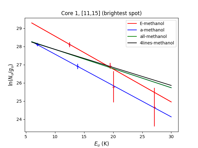
Figure 13: A comparison of methanol rotational diagrams toward the brightest pixel in core 1: based on E-methanol only (red line), based on A-methanol only (blue), based on all six A- and E-methanol lines including the weak higher energy lines (green), and based on the four A- and E-methanol lines (black, the one used to measure $N_{\rm tot}$). Red symbols show E-methanol, blue symbols show A-methanol.

Appendix B Additional figures

References

- Alonso-Albi et al. (2010) Alonso-Albi, T., Fuente, A., Crimier, N., et al. 2010, A&A, 518, A52, doi: 10.1051/0004-6361/201014317
- André et al. (2014) André, P., Di Francesco, J., Ward-Thompson, D., et al. 2014, Protostars and Planets VI, 27, doi: 10.2458/azu_uapress_9780816531240-ch002
- Astropy Collaboration et al. (2013) Astropy Collaboration, Robitaille, T. P., Tollerud, E. J., et al. 2013, A&A, 558, A33, doi: 10.1051/0004-6361/201322068
- Astropy Collaboration et al. (2018) Astropy Collaboration, Price-Whelan, A. M., Sipőcz, B. M., et al. 2018, AJ, 156, 123, doi: 10.3847/1538-3881/aabc4f
- Bacmann et al. (2002) Bacmann, A., Lefloch, B., Ceccarelli, C., et al. 2002, A&A, 389, L6, doi: 10.1051/0004-6361:20020652
- Barnard (1927) Barnard, E. E. 1927, Catalogue of 349 dark objects in the sky
- Beckwith et al. (1990) Beckwith, S. V. W., Sargent, A. I., Chini, R. S., & Guesten, R. 1990, AJ, 99, 924, doi: 10.1086/115385
- Benson & Myers (1989) Benson, P. J., & Myers, P. C. 1989, ApJS, 71, 89, doi: 10.1086/191365
- Bergin & Tafalla (2007) Bergin, E. A., & Tafalla, M. 2007, ARA&A, 45, 339, doi: 10.1146/annurev.astro.45.071206.100404
- Bertin et al. (2016) Bertin, M., Romanzin, C., Doronin, M., et al. 2016, ApJ, 817, L12, doi: 10.3847/2041-8205/817/2/L12
- Bizzocchi et al. (2014) Bizzocchi, L., Caselli, P., Spezzano, S., & Leonardo, E. 2014, A&A, 569, A27, doi: 10.1051/0004-6361/201423858
- Bracco et al. (2017) Bracco, A., Palmeirim, P., André, P., et al. 2017, A&A, 604, A52, doi: 10.1051/0004-6361/201731117
- Caselli et al. (1994) Caselli, P., Hasegawa, T. I., & Herbst, E. 1994, ApJ, 421, 206, doi: 10.1086/173637
- Caselli et al. (1999) Caselli, P., Walmsley, C. M., Tafalla, M., Dore, L., & Myers, P. C. 1999, ApJ, 523, L165, doi: 10.1086/312280
- Caselli et al. (1998) Caselli, P., Walmsley, C. M., Terzieva, R., & Herbst, E. 1998, ApJ, 499, 234, doi: 10.1086/305624
- Caselli et al. (2002) Caselli, P., Walmsley, C. M., Zucconi, A., et al. 2002, ApJ, 565, 344, doi: 10.1086/324302
- Chaabouni et al. (2012) Chaabouni, H., Bergeron, H., Baouche, S., et al. 2012, A&A, 538, A128, doi: 10.1051/0004-6361/201117409
- Chacón-Tanarro et al. (2017) Chacón-Tanarro, A., Caselli, P., Bizzocchi, L., et al. 2017, A&A, 606, A142, doi: 10.1051/0004-6361/201630265
- Chen et al. (2014) Chen, Y. J., Chuang, K. J., Muñoz Caro, G. M., et al. 2014, ApJ, 781, 15, doi: 10.1088/0004-637X/781/1/15
- Chuang et al. (2018) Chuang, K. J., Fedoseev, G., Qasim, D., et al. 2018, ApJ, 853, 102, doi: 10.3847/1538-4357/aaa24e
- Crapsi et al. (2005) Crapsi, A., Caselli, P., Walmsley, C. M., et al. 2005, ApJ, 619, 379, doi: 10.1086/426472
- Cruz-Diaz et al. (2016) Cruz-Diaz, G. A., Martín-Doménech, R., Muñoz Caro, G. M., & Chen, Y.-J. 2016, A&A, 592, A68, doi: 10.1051/0004-6361/201526761
- Draine & Li (2007) Draine, B. T., & Li, A. 2007, ApJ, 657, 810, doi: 10.1086/511055
- Fayolle et al. (2011) Fayolle, E. C., Bertin, M., Romanzin, C., et al. 2011, ApJ, 739, L36, doi: 10.1088/2041-8205/739/2/L36
- Fedoseev et al. (2015) Fedoseev, G., Cuppen, H. M., Ioppolo, S., Lamberts, T., & Linnartz, H. 2015, MNRAS, 448, 1288, doi: 10.1093/mnras/stu2603
- Fraser & van Dishoeck (2004) Fraser, H. J., & van Dishoeck, E. F. 2004, Advances in Space Research, 33, 14, doi: 10.1016/j.asr.2003.04.003
- Fredon et al. (2017) Fredon, A., Lamberts, T., & Cuppen, H. M. 2017, ApJ, 849, 125, doi: 10.3847/1538-4357/aa8c05
- Frerking et al. (1982) Frerking, M. A., Langer, W. D., & Wilson, R. W. 1982, ApJ, 262, 590, doi: 10.1086/160451
- Friesen et al. (2017) Friesen, R. K., Pineda, J. E., co-PIs, et al. 2017, ApJ, 843, 63, doi: 10.3847/1538-4357/aa6d58
- Fuchs et al. (2009) Fuchs, G. W., Cuppen, H. M., Ioppolo, S., et al. 2009, A&A, 505, 629, doi: 10.1051/0004-6361/200810784
- Garrod et al. (2006) Garrod, R., Park, I. H., Caselli, P., & Herbst, E. 2006, Faraday Discussions, 133, 51, doi: 10.1039/b516202e
- Garrod et al. (2007) Garrod, R. T., Wakelam, V., & Herbst, E. 2007, A&A, 467, 1103, doi: 10.1051/0004-6361:20066704
- Geppert et al. (2006) Geppert, W. D., Hamberg, M., Thomas, R. D., et al. 2006, Faraday Discussions, 133, 177, doi: 10.1039/B516010C
- Ginsburg & Mirocha (2011) Ginsburg, A., & Mirocha, J. 2011, PySpecKit: Python Spectroscopic Toolkit, Astrophysics Source Code Library. http://ascl.net/1109.001
- Goldsmith (2001) Goldsmith, P. F. 2001, ApJ, 557, 736, doi: 10.1086/322255
- Goldsmith & Langer (1999) Goldsmith, P. F., & Langer, W. D. 1999, ApJ, 517, 209, doi: 10.1086/307195
- Gordy & Cook (1970) Gordy, W., & Cook, R. L. 1970, Chemical applications of spectroscopy, Vol. 2, Microwave molecular spectra (New York u.a.: Interscience Publisher, 1970)
- Graedel et al. (1982) Graedel, T. E., Langer, W. D., & Frerking, M. A. 1982, ApJS, 48, 321, doi: 10.1086/190780
- Güver & Özel (2009) Güver, T., & Özel, F. 2009, MNRAS, 400, 2050, doi: 10.1111/j.1365-2966.2009.15598.x
- Hacar et al. (2013) Hacar, A., Tafalla, M., Kauffmann, J., & Kovács, A. 2013, A&A, 554, A55, doi: 10.1051/0004-6361/201220090
- Harju et al. (2017) Harju, J., Daniel, F., Sipilä, O., et al. 2017, A&A, 600, A61, doi: 10.1051/0004-6361/201628463
- Harju et al. (2020) Harju, J., Pineda, J. E., Vasyunin, A. I., et al. 2020, ApJ, 895, 101, doi: 10.3847/1538-4357/ab8f93
- Hasegawa & Herbst (1993) Hasegawa, T. I., & Herbst, E. 1993, MNRAS, 261, 83, doi: 10.1093/mnras/261.1.83
- Hasegawa et al. (1992) Hasegawa, T. I., Herbst, E., & Leung, C. M. 1992, ApJS, 82, 167, doi: 10.1086/191713
- Hasenberger & Alves (2020) Hasenberger, B., & Alves, J. 2020, A&A, 633, A132, doi: 10.1051/0004-6361/201936095
- Jiménez-Serra et al. (2021) Jiménez-Serra, I., Vasyunin, A. I., Spezzano, S., et al. 2021, ApJ, 917, 44, doi: 10.3847/1538-4357/ac024c
- Jiménez-Serra et al. (2016) Jiménez-Serra, I., Vasyunin, A. I., Caselli, P., et al. 2016, ApJ, 830, L6, doi: 10.3847/2041-8205/830/1/L6
- Jin & Garrod (2020) Jin, M., & Garrod, R. T. 2020, ApJS, 249, 26, doi: 10.3847/1538-4365/ab9ec8
- Jørgensen et al. (2002) Jørgensen, J. K., Schöier, F. L., & van Dishoeck, E. F. 2002, A&A, 389, 908, doi: 10.1051/0004-6361:20020681
- Keto & Caselli (2008) Keto, E., & Caselli, P. 2008, ApJ, 683, 238, doi: 10.1086/589147
- Keto & Caselli (2010) —. 2010, MNRAS, 402, 1625, doi: 10.1111/j.1365-2966.2009.16033.x
- Kirk et al. (2005) Kirk, J. M., Ward-Thompson, D., & André, P. 2005, MNRAS, 360, 1506, doi: 10.1111/j.1365-2966.2005.09145.x
- Laas & Caselli (2019) Laas, J. C., & Caselli, P. 2019, A&A, 624, A108, doi: 10.1051/0004-6361/201834446
- Lacy et al. (1994) Lacy, J. H., Knacke, R., Geballe, T. R., & Tokunaga, A. T. 1994, ApJ, 428, L69, doi: 10.1086/187395
- Lacy et al. (2017) Lacy, J. H., Sneden, C., Kim, H., & Jaffe, D. T. 2017, ApJ, 838, 66, doi: 10.3847/1538-4357/aa6247
- Ladjelate et al. (2020) Ladjelate, B., André, P., Könyves, V., et al. 2020, A&A, 638, A74, doi: 10.1051/0004-6361/201936442
- Lamberts & Kästner (2017) Lamberts, T., & Kästner, J. 2017, ApJ, 846, 43, doi: 10.3847/1538-4357/aa8311
- Lattanzi et al. (2020) Lattanzi, V., Bizzocchi, L., Vasyunin, A. I., et al. 2020, A&A, 633, A118, doi: 10.1051/0004-6361/201936884
- Lee et al. (1998) Lee, H. H., Roueff, E., Pineau des Forets, G., et al. 1998, A&A, 334, 1047
- Lee et al. (2003) Lee, J.-E., Evans, Neal J., I., Shirley, Y. L., & Tatematsu, K. 2003, ApJ, 583, 789, doi: 10.1086/345428
- Lees & Baker (1968) Lees, R. M., & Baker, J. G. 1968, The Journal of Chemical Physics, 48, 5299, doi: 10.1063/1.1668221
- Loison et al. (2020) Loison, J.-C., Wakelam, V., Gratier, P., & Hickson, K. M. 2020, MNRAS, 498, 4663, doi: 10.1093/mnras/staa2700
- Lynds (1962) Lynds, B. T. 1962, ApJS, 7, 1, doi: 10.1086/190072
- Marsh et al. (2014) Marsh, K. A., Griffin, M. J., Palmeirim, P., et al. 2014, MNRAS, 439, 3683, doi: 10.1093/mnras/stu219
- Minissale et al. (2016) Minissale, M., Moudens, A., Baouche, S., Chaabouni, H., & Dulieu, F. 2016, MNRAS, 458, 2953, doi: 10.1093/mnras/stw373
- Muñoz Caro et al. (2016) Muñoz Caro, G. M., Chen, Y. J., Aparicio, S., et al. 2016, A&A, 589, A19, doi: 10.1051/0004-6361/201628121
- Nagy et al. (2019) Nagy, Z., Spezzano, S., Caselli, P., et al. 2019, A&A, 630, A136, doi: 10.1051/0004-6361/201935568
- Öberg et al. (2009) Öberg, K. I., Garrod, R. T., van Dishoeck, E. F., & Linnartz, H. 2009, A&A, 504, 891, doi: 10.1051/0004-6361/200912559
- Paardekooper et al. (2016) Paardekooper, D. M., Fedoseev, G., Riedo, A., & Linnartz, H. 2016, A&A, 596, A72, doi: 10.1051/0004-6361/201629063
- Pagani et al. (2007) Pagani, L., Bacmann, A., Cabrit, S., & Vastel, C. 2007, A&A, 467, 179, doi: 10.1051/0004-6361:20066670
- Palmeirim et al. (2013) Palmeirim, P., André, P., Kirk, J., et al. 2013, A&A, 550, A38, doi: 10.1051/0004-6361/201220500
- Pickett et al. (1998) Pickett, H. M., Poynter, R. L., Cohen, E. A., et al. 1998, J. Quant. Spec. Radiat. Transf., 60, 883, doi: 10.1016/S0022-4073(98)00091-0
- Punanova et al. (2018a) Punanova, A., Caselli, P., Pineda, J. E., et al. 2018a, A&A, 617, A27, doi: 10.1051/0004-6361/201731159
- Punanova et al. (2018b) Punanova, A., Caselli, P., Feng, S., et al. 2018b, ApJ, 855, 112, doi: 10.3847/1538-4357/aaad09
- Rebull et al. (2010) Rebull, L. M., Padgett, D. L., McCabe, C.-E., et al. 2010, ApJS, 186, 259, doi: 10.1088/0067-0049/186/2/259
- Rimola et al. (2014) Rimola, A., Taquet, V., Ugliengo, P., Balucani, N., & Ceccarelli, C. 2014, A&A, 572, A70, doi: 10.1051/0004-6361/201424046
- Roccatagliata et al. (2020) Roccatagliata, V., Franciosini, E., Sacco, G. G., Rand ich, S., & Sicilia-Aguilar, A. 2020, A&A, 638, A85, doi: 10.1051/0004-6361/201936401
- Ruaud et al. (2016) Ruaud, M., Wakelam, V., & Hersant, F. 2016, MNRAS, 459, 3756, doi: 10.1093/mnras/stw887
- Santiago-García et al. (2009) Santiago-García, J., Tafalla, M., Johnstone, D., & Bachiller, R. 2009, A&A, 495, 169, doi: 10.1051/0004-6361:200810739
- Schlafly et al. (2014) Schlafly, E. F., Green, G., Finkbeiner, D. P., et al. 2014, ApJ, 786, 29, doi: 10.1088/0004-637X/786/1/29
- Schmalzl et al. (2010) Schmalzl, M., Kainulainen, J., Quanz, S. P., et al. 2010, ApJ, 725, 1327, doi: 10.1088/0004-637X/725/1/1327
- Schnee et al. (2010) Schnee, S., Enoch, M., Noriega-Crespo, A., et al. 2010, ApJ, 708, 127, doi: 10.1088/0004-637X/708/1/127
- Schöier et al. (2005) Schöier, F. L., van der Tak, F. F. S., van Dishoeck, E. F., & Black, J. H. 2005, A&A, 432, 369, doi: 10.1051/0004-6361:20041729
- Scibelli & Shirley (2020) Scibelli, S., & Shirley, Y. 2020, ApJ, 891, 73, doi: 10.3847/1538-4357/ab7375
- Scibelli et al. (2021) Scibelli, S., Shirley, Y., Vasyunin, A., & Launhardt, R. 2021, MNRAS, 504, 5754, doi: 10.1093/mnras/stab1151
- Seo et al. (2015) Seo, Y. M., Shirley, Y. L., Goldsmith, P., et al. 2015, ApJ, 805, 185, doi: 10.1088/0004-637X/805/2/185
- Seo et al. (2019) Seo, Y. M., Majumdar, L., Goldsmith, P. F., et al. 2019, ApJ, 871, 134, doi: 10.3847/1538-4357/aaf887
- Shalabiea (2001) Shalabiea, O. M. 2001, A&A, 370, 1044, doi: 10.1051/0004-6361:20010323
- Shingledecker et al. (2020) Shingledecker, C. N., Lamberts, T., Laas, J. C., et al. 2020, ApJ, 888, 52, doi: 10.3847/1538-4357/ab5360
- Sipilä et al. (2020) Sipilä, O., Zhao, B., & Caselli, P. 2020, A&A, 640, A94, doi: 10.1051/0004-6361/202038353
- Spezzano et al. (2016) Spezzano, S., Bizzocchi, L., Caselli, P., Harju, J., & Brünken, S. 2016, A&A, 592, L11, doi: 10.1051/0004-6361/201628652
- Spezzano et al. (2020) Spezzano, S., Caselli, P., Pineda, J. E., et al. 2020, A&A, 643, A60, doi: 10.1051/0004-6361/201936598
- Tafalla & Hacar (2015) Tafalla, M., & Hacar, A. 2015, A&A, 574, A104, doi: 10.1051/0004-6361/201424576
- Tafalla & Santiago (2004) Tafalla, M., & Santiago, J. 2004, A&A, 414, L53, doi: 10.1051/0004-6361:20031766
- Tafalla et al. (2006) Tafalla, M., Santiago-García, J., Myers, P. C., et al. 2006, A&A, 455, 577, doi: 10.1051/0004-6361:20065311
- Vastel et al. (2014) Vastel, C., Ceccarelli, C., Lefloch, B., & Bachiller, R. 2014, ApJ, 795, L2, doi: 10.1088/2041-8205/795/1/L2
- Vasyunin et al. (2017) Vasyunin, A. I., Caselli, P., Dulieu, F., & Jiménez-Serra, I. 2017, ApJ, 842, 33, doi: 10.3847/1538-4357/aa72ec
- Vasyunin & Herbst (2013a) Vasyunin, A. I., & Herbst, E. 2013a, ApJ, 769, 34, doi: 10.1088/0004-637X/769/1/34
- Vasyunin & Herbst (2013b) —. 2013b, ApJ, 762, 86, doi: 10.1088/0004-637X/762/2/86
- Wakelam & Herbst (2008) Wakelam, V., & Herbst, E. 2008, ApJ, 680, 371, doi: 10.1086/587734
- Wakelam et al. (2017) Wakelam, V., Loison, J. C., Mereau, R., & Ruaud, M. 2017, Molecular Astrophysics, 6, 22, doi: 10.1016/j.molap.2017.01.002
- Walsh et al. (2009) Walsh, C., Harada, N., Herbst, E., & Millar, T. J. 2009, ApJ, 700, 752, doi: 10.1088/0004-637X/700/1/752
- Wannier (1980) Wannier, P. G. 1980, ARA&A, 18, 399, doi: 10.1146/annurev.aa.18.090180.002151
- Ward-Thompson et al. (2016) Ward-Thompson, D., Pattle, K., Kirk, J. M., et al. 2016, MNRAS, 463, 1008, doi: 10.1093/mnras/stw1978
- Watanabe & Kouchi (2002) Watanabe, N., & Kouchi, A. 2002, ApJ, 571, L173, doi: 10.1086/341412
- Whittet et al. (2011) Whittet, D. C. B., Cook, A. M., Herbst, E., Chiar, J. E., & Shenoy, S. S. 2011, ApJ, 742, 28, doi: 10.1088/0004-637X/742/1/28
- Willacy et al. (1998) Willacy, K., Langer, W. D., & Velusamy, T. 1998, ApJ, 507, L171, doi: 10.1086/311695
- Wilson & Rood (1994) Wilson, T. L., & Rood, R. 1994, ARA&A, 32, 191, doi: 10.1146/annurev.aa.32.090194.001203
- Wirström et al. (2011) Wirström, E. S., Geppert, W. D., Hjalmarson, Å., et al. 2011, A&A, 533, A24, doi: 10.1051/0004-6361/201116525
- Xu & Lovas (1997) Xu, L.-H., & Lovas, F. J. 1997, Journal of Physical and Chemical Reference Data, 26, 17, doi: 10.1063/1.556005