Correlating confinement to topological fluctuations near the crossover transition in QCD

Abstract

We show the existence of strong (anti)correlations between the topological hot spots and the local values of the trace of the Polyakov loop in $2+1$ flavor QCD with physical quark mass, in the vicinity of the crossover transition corresponding to the simultaneous restoration of chiral symmetry and deconfinement. Using sophisticated lattice techniques, we have carefully identified the topological hot spots using quark zero modes and measured the short-distance fluctuations of the Polyakov loop about them, showing how the latter is repelled quite strongly around the peak of the zero modes. Though we could explain some aspects of these correlations within the instanton-dyon picture, our work sets the stage for a larger goal towards a systematic study of the role of different topological species that interact with the Polyakov loop, establishing the strong connection between topology and confinement.

I Introduction

The two most important nonperturbative phenomena in Quantum Chromodynamics (QCD) are chiral symmetry breaking and confinement  Ding:2015ona ; Schmidt:2017bjt ; Lombardo:2020bvn . The corresponding order parameters are (the nonzero value of) the quark condensate $\langle\bar{q}q\rangle\neq 0$ and the (vanishingly small) expectation value of the Polyakov loop $\langle\text{Tr}[P(\vec{x})]\rangle/3=0$. Many authors have debated whether and how precisely these two phenomena can be related, see for e.g.  Shuryak:1982hk ; Shuryak:2014gja ; Larsen:2015vaa ; Larsen:2015tso ; Bazavov:2016uvm ; Clarke:2020htu ; DeMartini:2021xkg . In this Letter, we address this fundamental question at the local level, using gauge configurations from lattice simulations of $2+1$ flavor QCD, by correlating the location of the maxima of zero modes of the Dirac operator with the local minima of the Polyakov loop.

Furthermore, it is now widely believed that both of these phenomena are driven by gauge topology Schafer:1996wv . In order to produce confinement, the topological objects need to interact with $P(\vec{x})$ locally and suppress it, in the confined phase at $T\lesssim T_{c}$, where $T_{c}$ is the chiral crossover-transition temperature Borsanyi:2010bp ; Bazavov:2011nk ; Bhattacharya:2014ara ; Burger:2018fvb ; Bazavov:2018mes . With increasing temperatures, the density of these topological objects gets small, but still to a certain extent suppress the local fluctuations of $P(\vec{x})$. In $3+1$ dimensions, instantons do not couple to the Polyakov loop, though it was historically introduced to explain confinement in $2+1$ dimensions Polyakov:1976fu . Several other candidates have been considered in literature which include vortices  Nielsen:1973cs ; Mandelstam:1974pi ; Engelhardt:2004pf ; Greensite:2016pfc , monopoles tHooft:1981bkw ; Polikarpov:1996wd ; DiGiacomo:1999yas ; Bonati:2011jv , and the constituents of instantons, the so-called instanton-dyons Kraan:1998sn ; Lee:1998bb ; Kraan:1998pm . Well separated isolated instanton-dyons are simply three-dimensional monopoles, for which the gauge potential $A_{4}(\vec{x})$ plays the role of the adjoint Higgs field. In Euclidean finite temperature formulation, it may have a nonzero average value, resulting in a nontrivial holonomy. A similar to magnetic monopoles, instanton-dyons repel the Higgs field at their centers. Therefore one expects to see a difference between the average value of the Polyakov loop and its local value at the center of an instanton-dyon. Similar picture exists in the core of the vortices. However, in order to really identify those and quantify the role which each of them plays, one can only rely on first principles lattice QCD calculations.

The main objective of this Letter is to unambiguously identify the correlations, if any, between the position of the topological zero modes of the QCD Dirac operator and the local value of the Polyakov loop. We focus on a temperature range just beyond the chiral crossover transition where the connection between the zeromodes to a semiclassical ensemble of instanton-dyons has been shown previously Gonzalez-Arroyo:1995isl ; Gonzalez-Arroyo:1995ynx ; GarciaPerez:1999hs ; Bornyakov:2013iva ; Larsen:2018crg ; Larsen:2019sdi . However the observables we suggest here and techniques which we have developed in order to reliably measure the correlations is very general and does not rely upon the existence of any specific topological ensemble. We discuss the numerical setup in the next section followed by our specific proposal of different observables in the subsequent section that helps one to reliably establish the sensitivity of the hot spots of topological fluctuations to the local minima of the Polyakov loop. We finally conclude with the deeper implications of our work, of how it impacts our understanding of the role of topology in explaining confinement in gauge theories.

II Methodology

For success of such a study it is crucial that we use lattice fermions with the best chiral properties on the lattice. This includes maintaining an exact index theorem on the lattice, by which one can identify the topological objects through the zero modes of the QCD Dirac operator. It is also important that the gauge ensembles generated using dynamical fermions also preserve the chiral properties of the latter, without which there could be artifacts of explicit chiral symmetry breaking. The gauge configurations used in this work are $2+1$ flavor QCD configurations generated by the HotQCD Collaboration Bhattacharya:2014ara using the Möbious domain wall discretization Kaplan:1992bt ; Brower:2012vk for fermions and Iwasaki gauge action. The residual chiral violation of the configurations generated using Möbius domain wall fermions is tiny, of the order of $\sim 2\times 10^{-3}$. We have used overlap fermions Narayanan:1994gw ; Neuberger:1998my as the probe to measure the topological content of the sea-gauge ensembles since the domain wall fermions do not satisfy an exact index theorem on the lattice. The zero modes of the valence overlap Dirac operator can be identified with the topological objects of the underlying gauge configurations Berruto:2000fx since it satisfies an exact index theorem, even at finite lattice spacings Hasenfratz:1998ri .

The overlap Dirac operator is defined as $D=1-\gamma_{5}sign(H_{W})$ where the kernel of the sign function is $H_{W}=\gamma_{5}(M-aD_{W})$, $D_{W}$ being the massless Wilson-Dirac operator Wilson:1974sk . $M$ is the domain wall height which is chosen to be in the interval $[0,2)$ to simulate one massless quark flavor on the lattice. The overlap operator satisfies the Ginsparg-Wilson relation Ginsparg:1981bj , $\gamma_{5}D^{-1}+D^{-1}\gamma_{5}=a\gamma_{5}$ which is numerically implemented to a precision of $10^{-10}$. Furthermore we studied the eigenspectrum of the overlap operator by varying the periodicity phase $\phi$ of the valence overlap Dirac fields along the temporal torus, defined as $\psi(\tau+1/T)=\rm{e}^{i\phi}\psi(\tau)$. We can then identify different species of instanton-dyons with the Dirac zero modes corresponding to the phases $\phi$, following the procedure outlined in Gattringer:2002wh ; Larsen:2019sdi .

We have also carefully chosen fairly large volume lattices for our study since the topological content of the gauge field ensembles are sensitive to finite volume effects. The Euclidean space-time lattice has $N_{s}=32$ sites along each of spatial direction and $N_{\tau}=8$ sites along the temporal direction. The spatial volume in physical units is $\sim(4~{}\text{fm})^{3}$, each spatial extent about four times the pion Compton wavelength. The quark masses are tuned to their physical values corresponding to a Goldstone pion and kaon mass of $135$ and $435$ MeV respectively. We have performed the study at two different temperatures $1.1~{}T_{c}$ and $1.2~{}T_{c}$, where the number of independent configurations with topological charge $|Q|=1$ are $5,12$ respectively. For this specific $Q$ sector the zero modes are particularly easier to locate precisely, which is important for finding its correlations with the gauge observables. We have not considered the other $|Q|>1$ sectors in this work since identifying the zero mode for different boundary angles is nontrivial, and we will address this topic separately. Moreover, the number of configurations with $|Q|>1$ was small for the higher temperature ensembles and we therefore do not expect the exclusion of these configurations to strongly impact our results.

The pseudocritical temperature $T_{c}=155(9)$ MeV for these ensembles Bhattacharya:2014ara . Moreover for these two temperatures the lattice spacings are fine enough in the range $\sim 0.13$-$0.14$ fm, to ensure that cutoff effects are under control.

III Observables

The aim of this work is to specifically look for correlations between topological zero modes and confinement, and our suggested techniques are very general, irrespective of the specific nature of the topological objects. However we will show some tantalizing connections to some of our earlier studies on instanton-dyons  Larsen:2018crg ; Larsen:2019sdi in the next section.

Instanton-dyons, also called instanton-monopoles are one of the attractive candidates which may explain confinement Diakonov:2009jq . For $SU(N_{c})$ gauge theory at finite temperature, instanton-dyons naturally arise as the substructures of instanton solutions in presence of a finite holonomy, also known as Kraan-van Baal-Lu-Liu calorons Kraan:1998sn ; Lee:1998bb ; Kraan:1998pm ; Gonzalez-Arroyo:2019wpu . Several lattice studies have reported the presence of dyons in pure gauge theories  GarciaPerez:1999ux ; Chernodub:1999wg ; Gattringer:2002wh ; Bornyakov:2014esa as well as in QCD Bornyakov:2015xao ; Bornyakov:2016ccq . Using sophisticated fits to lattice data, it is now possible to identify the different species of instanton-dyons and measure their typical separations as a function of temperature Larsen:2019sdi . Clusters of local topological fluctuations identified using a local definition of topological charge constructed out of the eigenvectors of the valence Dirac operator with generalized periodicity phases, have been observed to be correlated with the timelike monopole currents in $SU(3)$ gauge theory, defined in the maximal Abelian gauge Bornyakov:2014esa . Furthermore scatter plots of the real and imaginary parts of the Polyakov loop in the center of these clusters Bornyakov:2014esa further hinted at a deeper connection between these topological excitations and the Polyakov loop.

The local Polyakov loop or the holonomy is defined as the product over the temporal links as $P(\vec{x})=\Pi_{x_{4}=1}^{N_{\tau}}U_{4}(\vec{x},x_{4})$ whose $k$-th eigenvalue, $k\in[1,N_{c}]$ is simply $\rm{e}^{2i\pi\mu_{k}(\vec{x})}$. Measuring this observable at each spacetime point is quite a challenging task as it has large contributions from the ultraviolet fluctuations of the gauge fields. We use $10$ steps of hypercubic (HYP) smearing Hasenfratz:2001hp to remove these ultraviolet fluctuations. With this choice of smearing we improved the signal-to-noise ratio sufficiently to measure its local values. We introduce an observable which measures how well the local Polyakov loop operator on smeared gauge ensembles correlate with the fermion zero mode density which is defined as,

$$C(\Delta P,\rho)=\int d^{3}\vec{x}~{}\rho(\vec{x})~{}\frac{1}{3}\big{[}\text{Tr}[P(\vec{x})]-\langle\text{Tr}[P(\vec{x})]\rangle\big{]}~{}.$$ (1)

In our previous works Larsen:2018crg ; Larsen:2019sdi , we have shown that the fermionic zero modes are remarkably insensitive to the ultraviolet noise due to the higher momentum modes of the gauge fields. We take advantage of this fact through our choice of this observable.

IV Are topological fluctuations in QCD above $T_{c}$ correlated to confinement?

We first measure the local density of the fermion zero-mode wave functions and compare with the density profile of the trace of the Polyakov loop operator measured on smeared gauge ensembles. The results of such a comparison for a typical QCD configuration at $1.1$ and $1.2~{}T_{c}$, for the usual antiperiodic boundary phase along the temporal direction, are shown in Fig. 1. We have shown the two dimensional profiles of the quark zero modes along the $x,y$ coordinates (blue) superimposed over the local variation of the Polyakov loop shown in yellow. In all these plots the $z$ coordinate is fixed to its value at the maxima of the zero mode and the temporal direction is integrated out. We do indeed observe that the local Polyakov loop value drops strongly to negative values precisely at the location of the maxima of the zero modes which correspond to $L$-dyons i.e. for the boundary phase $\phi=\pi$. This nice visual correlation is quite robust, and exists for all temperatures above $T_{c}$ we have studied. We also see other minima of the local Polyakov loop; some of them might correspond to locations of other species of instanton- dyons, but some perhaps to other topological objects e.g. vortices connecting them. We have not systematically investigated their origin, leaving it for a future study.

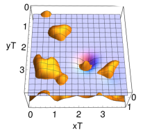
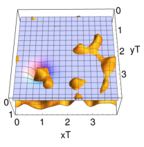
Figure 1: Typical snapshots of the inverted spatial density $\rho(\vec{x})$ of the fermion zero mode at $\phi=\pi$ (blue) superimposed on the spacetime profile of the inverted (real part of) Polyakov loop $\text{Tr}[P(\vec{x})]/3$ (yellow), measured after smearing the $2+1$ flavor QCD gauge configurations at $1.2~{}T_{c}$ (above) and $1.1~{}T_{c}$ (below) respectively. The flat blue sheet corresponds to the zero baseline and the only zero mode is visible as a crater on this surface. Each plot shows that the zero mode coincides with the most localized fluctuation of the Polyakov loop.

Though in Fig. 1 we have shown snapshots of correlations between the (real part of) Polyakov loop and topological zero modes for two configurations only, this strong correlation itself is very prevalent. It is present in all the configurations, at each temperature which we have studied so far and also for other quark periodicity phases $\phi=\pm\pi/3$. In order to bring out the cumulative information, we measure the observable $C(\Delta P,\rho)$ introduced in Eq. (1), which is averaged over all independent gauge ensembles we have examined. The typical values of the real and imaginary parts of $C(\Delta P,\rho)$ as a function of the fermion temporal phases are shown in Fig. 2. Whereas its imaginary part stays close to zero for all three values of temporal boundary phases as expected, the real part is distinctly finite and negative. This again establishes the fact that local Polyakov loop values drop strongly at the center of the topological hot spots, but now at a cumulative level for all gauge ensembles at $T\gtrsim T_{c}$.

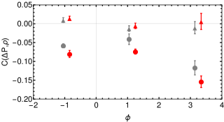
Figure 2: The real and imaginary parts of $C(\Delta P,\rho)$ defined in Eq. (1) shown as filled circles and triangles respectively for three different fermion boundary phases $\phi=\pi,\pm\pi/3$. The data points corresponding to temperatures $1.1~{}T_{c}$ and $1.2~{}T_{c}$ are shown in gray and red respectively and the points in red are shifted along the horizontal axis for the sake of clarity.

After demonstrating strong (anti)correlations between local hot spots of Polyakov loop with the topological fluctuations, we turn to some observations specific to the instanton-dyon formalism. This is motivated from the fact that the average values of the Polyakov loop at these temperatures have been shown previously to be quite accurately explained due to weakly interacting semiclassical gas of instanton-dyons Larsen:2019sdi .

Each constituent dyon has its own Higgsing through a certain color projection of the local Polyakov loop, and we study whether such a property can be seen in the gauge configurations. The Polyakov loop far away from the topological hot spots, also known as the holonomy, can be represented as a diagonal matrix $\rm{exp}[2i\pi\text{diag}(\mu_{0},\mu_{1},\mu_{2})]$. The constituent instanton-dyon actions are fractions of the total instanton action given as $8\pi^{2}\nu_{m}/g^{2}$, where $\nu_{m}=\mu_{m+1}-\mu_{m}$ represents the fractions of the circle on which the eigenvalues of the holonomy are located. For the gauge group $SU(3)$, there are three of them with $m=0$-$2$ and $\mu_{3}=1+\mu_{0}$.

Furthermore if instanton-dyons are well separated, the local holonomy at the position of the $i$-th dyon can be written as $P(\vec{x_{i}})=\text{diag}\left[\rm{e}^{i2\pi\mu_{i-1}},\rm{e}^{i\pi(\mu_{i}+\mu_{i+1})},\rm{e}^{i\pi(\mu_{i}+\mu_{i+1})}\right]$  Diakonov:2009jq . In the confined phase at $T\lesssim T_{c}$, where the average Polyakov loop is vanishingly small, the instanton action is split evenly between its constituent instanton-dyons, $\nu_{0}=\nu_{1}=\nu_{2}=1/3$, resulting in $\mu_{0}=0,\mu_{1}=1/3$ and $\mu_{2}=2/3$. The Polyakov loop operator near the fermion zero mode corresponding to the $L$-dyon with temporal periodicity phase $\phi=\pi$ (which normalized by $2\pi$ lies between $\mu_{1}$ and $\mu_{2}$), is $P(\vec{x}_{1})=\text{diag}[1,-1,-1]$. Taking a color trace and normalizing by the color factor, the imaginary part of the local Polyakov loop is zero, whereas its real part is $-1/3$. For the two M dyons which correspond to temporal boundary phases $\phi=\pm\pi/3$, the values of the local holonomy at its location are $1/6\pm i/\sqrt{12}$.

We next measure the real and the imaginary parts of the Polyakov loop $\text{Tr}[P(\vec{x})]/3$ as a function of the distance from the center of the fermion zero modes belonging to specific species of instanton-dyons, for each gauge configuration and subsequently performing a statistical average over all the configurations studied. The results for these observables at $T=1.2~{}T_{c}$ are shown in Fig. 3 for three different temporal phases for the valence fermions corresponding to the $L$ (top panel) and two different species of $M$ dyons (mid and lower panels) respectively. For $L$ dyons, we observe that the real part of the local Polyakov loop at its center (which is the origin of the plots) is negative, whereas its imaginary part is consistent with zero. At distances far away from the peak of the zero mode the real part of the local value of the Polyakov loop approaches its average value, while the imaginary part remains close to zero. These results are consistent with the expectations from a weakly interacting instanton-dyon model close to the confining phase. Contrasting this with the behavior of the local Polyakov loop for temporal boundary phases $\phi=\pm\pi/3$, we find that its real part shows an upward trend from negative towards zero, respectively. The central value of the imaginary part on the other hand, changes sign when changing between these two boundary phases, albeit large statistical errors. The data shows that the behavior of the local Polyakov loop deviates from the expectation of a weakly interacting gas more so for $M$ dyons as compared to $L$ dyons. This can be due to the fact that the average Polyakov loop is not negligibly small at $1.2~{}T_{c}$ and a semiclassical description of instanton-dyon gas may no longer be good. With increased statistics, the imaginary part of the local Polyakov loop might provide a better understanding of the interactions between the different species of instanton-dyons.

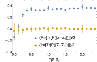
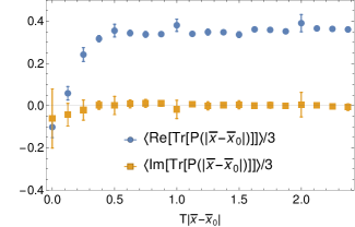
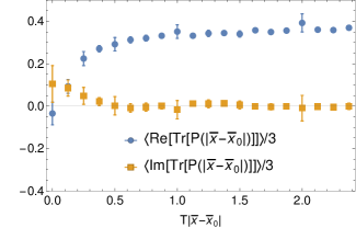
Figure 3: The variation of the real and imaginary parts of the Polyakov loop $\text{Tr}[P(\vec{x})]/3$ at $1.2~{}T_{c}$ for temporal boundary phases $\phi=\pi$ (top), $\phi=\pi/3$ (middle) and $\phi=-\pi/3$ (bottom) with the three-dimensional distance from the maximum of the fermionic zero modes.

V Summary & Outlook

In this Letter we have shown that there exists strong (anti)correlations between the topological hot spots (which can be identified as instanton-dyons ) and the confinement order parameter $\langle\text{Tr}[P(\vec{x})]/3\rangle$ at temperatures $T\gtrsim T_{c}$. Moreover, it is a local effect. Revealing such correlations at a local level was made possible due to a combination of two novel techniques we have used. First was the efficient identification of the topological zero modes of the noisy $2+1$ flavor QCD ensembles. Although they were generated using domain-wall fermion discretization for the quarks with a relatively good chiral property, we identified its zero modes with valence overlap Dirac operator to make use of the exact index theorem for the latter.

Secondly we have successfully isolated the localized fluctuations of the Polyakov loop from the noisy large-scale fluctuations via well-tuned smearing techniques. Our study provides a first glimpse of how topological fluctuations due to, for e.g., instanton-dyons can result in suppressing the Polyakov loop values. In order to understand how topology drives confinement at a more quantitative level, we would like to extend this work towards identifying the role of other topological objects and their interactions. Such a study will quantify from first principles, the origin of confinement, as driven by gauge topology in its various forms.

References

- (1) H. T. Ding, F. Karsch and S. Mukherjee, Int. J. Mod. Phys. E 24, no.10, 1530007 (2015) [arXiv:1504.05274 [hep-lat]].
- (2) C. Schmidt and S. Sharma, J. Phys. G 44, no. 10, 104002 (2017) [arXiv:1701.04707 [hep-lat]].
- (3) M. P. Lombardo and A. Trunin, Int. J. Mod. Phys. A 35, no.20, 2030010 (2020) [arXiv:2005.06547 [hep-lat]].
- (4) E. V. Shuryak, Nucl. Phys. B 203, 140-156 (1982)
- (5) E. Shuryak, Nucl. Phys. A 928, 138-143 (2014) [arXiv:1401.2032 [nucl-th]].
- (6) R. Larsen and E. Shuryak, Phys. Rev. D 92, no. 9, 094022 (2015). [arXiv:1504.03341 [hep-ph]].
- (7) R. Larsen and E. Shuryak, Phys. Rev. D 93, no. 5, 054029 (2016). [arXiv:1511.02237 [hep-ph]].
- (8) A. Bazavov, N. Brambilla, H.-T. Ding, P. Petreczky, H.-P. Schadler, A. Vairo and J. H. Weber, Phys. Rev. D 93, no. 11, 114502 (2016) [arXiv:1603.06637 [hep-lat]].
- (9) D. A. Clarke, O. Kaczmarek, F. Karsch, A. Lahiri and M. Sarkar, Phys. Rev. D 103, no.1, L011501 (2021) [arXiv:2008.11678 [hep-lat]].
- (10) D. DeMartini and E. Shuryak, Phys. Rev. D 104, no.9, 094031 (2021) [arXiv:2108.06353 [hep-ph]].
- (11) T. Schaefer and E. V. Shuryak, Rev. Mod. Phys. 70, 323 (1998). [hep-ph/9610451].
- (12) S. Borsanyi et al. [Wuppertal-Budapest], JHEP 09, 073 (2010) [arXiv:1005.3508 [hep-lat]].
- (13) A. Bazavov et al., Phys. Rev. D 85, 054503 (2012). [arXiv:1111.1710 [hep-lat]].
- (14) T. Bhattacharya et al., Phys. Rev. Lett. 113, no. 8, 082001 (2014). [arXiv:1402.5175 [hep-lat]].
- (15) F. Burger, E. M. Ilgenfritz, M. P. Lombardo and A. Trunin, Phys. Rev. D 98, no.9, 094501 (2018) [arXiv:1805.06001 [hep-lat]].
- (16) A. Bazavov et al. [HotQCD Collaboration], Phys. Lett. B 795, 15 (2019) [arXiv:1812.08235 [hep-lat]].
- (17) A. M. Polyakov, Nucl. Phys. B 120, 429 (1977).
- (18) H. B. Nielsen and P. Olesen, Nucl. Phys. B 61, 45-61 (1973)
- (19) S. Mandelstam, Phys. Rept. 23, 245-249 (1976)
- (20) M. Engelhardt, Nucl. Phys. B Proc. Suppl. 140, 92-105 (2005) [arXiv:hep-lat/0409023 [hep-lat]].
- (21) J. Greensite, EPJ Web Conf. 137, 01009 (2017) [arXiv:1610.06221 [hep-lat]].
- (22) G. ’t Hooft, Nucl. Phys. B 190, 455-478 (1981)
- (23) M. I. Polikarpov, Nucl. Phys. B Proc. Suppl. 53, 134-140 (1997) [arXiv:hep-lat/9609020 [hep-lat]].
- (24) A. Di Giacomo, B. Lucini, L. Montesi and G. Paffuti, Phys. Rev. D 61, 034503 (2000) [arXiv:hep-lat/9906024 [hep-lat]].
- (25) C. Bonati, G. Cossu, M. D’Elia and A. Di Giacomo, Phys. Rev. D 85, 065001 (2012) [arXiv:1111.1541 [hep-lat]].
- (26) T. C. Kraan and P. van Baal, Phys. Lett. B 435, 389 (1998). [hep-th/9806034].
- (27) K. M. Lee and C. h. Lu, Phys. Rev. D 58, 025011 (1998). [hep-th/9802108].
- (28) T. C. Kraan and P. van Baal, Nucl. Phys. B 533, 627 (1998). [hep-th/9805168].
- (29) A. Gonzalez-Arroyo, P. Martinez and A. Montero, Phys. Lett. B 359, 159-165 (1995) [arXiv:hep-lat/9507006 [hep-lat]].
- (30) A. Gonzalez-Arroyo and P. Martinez, Nucl. Phys. B 459, 337-354 (1996) [arXiv:hep-lat/9507001 [hep-lat]].
- (31) M. Garcia Perez, A. Gonzalez-Arroyo, A. Montero and P. van Baal, JHEP 9906, 001 (1999) [hep-lat/9903022].
- (32) V. G. Bornyakov, E.-M. Ilgenfritz, B. V. Martemyanov, V. K. Mitrjushkin and M. Mueller-Preussker, Phys. Rev. D 87, no. 11, 114508 (2013) [arXiv:1304.0935 [hep-lat]].
- (33) R. N. Larsen, S. Sharma and E. Shuryak, Phys. Lett. B 794, 14 (2019) [arXiv:1811.07914 [hep-lat]].
- (34) R. N. Larsen, S. Sharma and E. Shuryak, Phys. Rev. D 102 (2020) no.3, 034501 [arXiv:1912.09141 [hep-lat]].
- (35) D. B. Kaplan, Phys. Lett. B 288, 342 (1992).
- (36) R. C. Brower, H. Neff and K. Orginos, Comput. Phys. Commun. 220, 1 (2017).
- (37) R. Narayanan and H. Neuberger, Nucl. Phys. B 443, 305 (1995). [hep-th/9411108].
- (38) H. Neuberger, Phys. Rev. Lett. 81, 4060 (1998). [hep-lat/9806025].
- (39) F. Berruto, R. Narayanan and H. Neuberger, Phys. Lett. B 489, 243-250 (2000) [arXiv:hep-lat/0006030 [hep-lat]].
- (40) P. Hasenfratz, V. Laliena and F. Niedermayer, Phys. Lett. B 427, 125 (1998). [hep-lat/9801021].
- (41) K. G. Wilson, Phys. Rev. D 10, 2445-2459 (1974)
- (42) P. H. Ginsparg and K. G. Wilson, Phys. Rev. D 25, 2649 (1982).
- (43) C. Gattringer, Phys. Rev. D 67, 034507 (2003). [hep-lat/0210001].
- (44) D. Diakonov, Nucl. Phys. B Proc. Suppl. 195 (2009), 5-45 [arXiv:0906.2456 [hep-ph]].
- (45) A. González-Arroyo, JHEP 02, 137 (2020) [arXiv:1910.12565 [hep-th]].
- (46) M. Garcia Perez, A. Gonzalez-Arroyo, C. Pena and P. van Baal, Phys. Rev. D 60, 031901 (1999) [hep-th/9905016].
- (47) M. N. Chernodub, T. C. Kraan and P. van Baal, Nucl. Phys. Proc. Suppl. 83, 556 (2000) [hep-lat/9907001].
- (48) V. G. Bornyakov, E. M. Ilgenfritz, B. V. Martemyanov and M. Muller-Preussker, Phys. Rev. D 91, no.7, 074505 (2015) [arXiv:1410.4632 [hep-lat]].
- (49) V. G. Bornyakov, E.-M. Ilgenfritz, B. V. Martemyanov and M. Muller-Preussker Phys. Rev. D 93, no. 7, 074508 (2016). [arXiv:1512.03217 [hep-lat]].
- (50) V. G. Bornyakov et al., EPJ Web Conf. 137, 03002 (2017). [arXiv:1611.07789 [hep-lat]].
- (51) A. Hasenfratz and F. Knechtli, Phys. Rev. D 64, 034504 (2001) [hep-lat/0103029].
- (52) M. A. Clark, R. Babich, K. Barros, R. C. Brower and C. Rebbi, Comput. Phys. Commun. 181, 1517 (2010). [arXiv:0911.3191 [hep-lat]].