Canonical Representations for Direct Generation of Strategies in High-level Petri Games

Abstract

Petri games are a multi-player game model for the synthesis of distributed systems with multiple concurrent processes based on Petri nets. The processes are the players in the game represented by the token of the net. The players are divided into two teams: the controllable system and the uncontrollable environment. An individual controller is synthesized for each process based only on their locally available causality-based information. For one environment player and a bounded number of system players, the problem of solving Petri games can be reduced to that of solving Büchi games.

High-level Petri games are a concise representation of ordinary Petri games. Symmetries, derived from a high-level representation, can be exploited to significantly reduce the state space in the corresponding Büchi game. We present a new construction for solving high-level Petri games. It involves the definition of a unique, canonical representation of the reduced Büchi game. This allows us to translate a strategy in the Büchi game directly into a strategy in the Petri game. An implementation applied on six structurally different benchmark families shows in almost all cases a performance increase for larger state spaces.

Canon. Representations for Direct Gen. of Strategies in High-level Petri Games

1 Introduction

Whether telecommunication networks, electronic banking, or the world wide web, distributed systems are all around us and are becoming increasingly more widespread. Though an entire system may appear as one unit, the local controllers in a network often act autonomously on only incomplete information to avoid constant communication. These independent agents must behave correctly under all possible uncontrollable behavior of the environment. Synthesis [2] avoids the error-prone task of manually implementing such local controllers by automatically generating correct ones from a given specification (or stating the nonexistence of such controllers). In case of a single process in the underlying model, synthesis approaches have been successfully applied in nontrivial applications (e.g., [3], [4]). Due to the incomplete information in systems with multiple processes progressing on their individual rate, modeling asynchronous distributed systems is even more cumbersome and particularly benefits from a synthesis approach.

Petri games [5] (based on an underlying Petri net [6] where the tokens are the players in the game) are a well-suited multi-player game model for the synthesis of asynchronous distributed systems because of its subclasses with comparably low complexity results. For Petri games with a single environment (uncontrollable) player, a bounded number of system (controllable) players, and a safety objective, i.e., all players have to avoid designated bad places, deciding the existence of a winning strategy for the system players is exptime-complete [7]. This problem is called the realizability problem. The result is obtained via a reduction to a two-player Büchi game with enriched markings, so called decision sets, as states.

High-level Petri nets [8] can concisely model large distributed systems. Correspondingly, high-level Petri games [9] are a concise high-level representation of ordinary Petri games. For solving high-level Petri games, the symmetries [10] of the system can be exploited to build a symbolic Büchi game with a significantly smaller number of states [11]. The states are equivalence classes of decision sets and called symbolic decision sets. For generating a Petri game strategy in a high-level Petri game the approach proposed in [11] resorts to the original strategy construction in [7], i.e., the equivalence classes of a symbolic two-player strategy are dissolved and a strategy for the standard two-player game is generated. Figure 1 shows in the two bottom layers the relation of the elements just described.

Figure 1: An overview of the scope of this paper. The connections between the different elements describe their interplay and where these methods are introduced. The connections labeled with “solve” mean that a two-player (Büchi) game can be solved by standard algorithms in game theory (e.g., [12]). The bottom level corresponds to the original reduction in [7], the level above corresponds to the high-level counterparts described in [9, 11], and the top level contains the elements introduced in this paper. The new reduction is marked by thick edges.

In this paper, we propose a new construction for solving high-level Petri games to avoid this detour while generating the strategy. In [11] the symbolic Büchi game is generated by comparing each newly added state with all already added ones for equivalence, i.e., the orbit problem must be answered. The new approach calculates a canonical representation for each newly added state (the constructive orbit problem [13]), and only stores these representations. This generation of a symbolic Büchi game with canonical representations is based on the corresponding ideas for reachability graphs from [14]. As in [11], we consider safe Petri games with a high-level representation, and exclude Petri games where the system can proceed infinitely without the environment. For the decidability result we consider, as in [7], Petri games with only one environment player, i.e., in every reachable marking there is at most one token on an environment place.

One of the main advantages of the new approach is that the canonical representations allow to directly generate a Petri game strategy from a symbolic Büchi game strategy without explicitly resolving all symmetries (cp. thick edges and the top level in Fig. 1).

((a)) High-level Petri game $\mathit{G}$

((b)) The represented P/T Petri game $\mathsf{G}=\mathsf{L}(\mathit{G})$.

Figure 2: Client/Server: The environment decides on one out of three computers to host a server. The system players (computers) can win the game by getting informed on the decision of the environment and connecting correctly.

Another advantage is the complexity for constructing the symbolic Büchi game. Even though the calculation of the canonical representation comes with a fixed cost, less comparisons can be necessary, depending on the input system. We implemented the new algorithm and applied our tool on the benchmark families used in [11] and Example 1.1. The results show in general a performance increase with an increasing number of states for almost all benchmark families.

We now introduce the example on which we demonstrate the successive development stages of the presented techniques throughout the paper.

Example 1.1

The high-level Petri game $\mathit{G}$ depicted in Fig. 2(a) models a simplified scenario where one out of three computers must host a server for the others to connect to. The environment nondeterministically decides which computer must be the host. The places in the net are partitioned into system places (gray) and environment places (white). An object on a place is a player in the corresponding team. Bad places are double-bordered. The variables $x,y$ on arcs are bound only locally to the transitions, and an assignment of objects to these variables is called a mode of the transition.

The environment player $\bullet$, initially residing on place $\mathit{Env}$, decides via transition $d$ in mode $x=\tilde{c}$ on a computer $\tilde{c}$ that should host the server. The system players (computers $c_{1},c_{2},c_{3}\in C_{1}$), initially residing on place $\mathit{Sys}$, can either directly, individually connect themselves to another computer $c^{\prime}$ via transition $\mathit{a}$ in mode $[y=c_{i},x=\tilde{c}]$, or wait for transition $\mathit{inf}$ to be enabled. When they choose to connect themselves directly, after firing transition $\mathit{a}$ in different modes, the corresponding pairs of computers reside on place $\mathit{A}$. Since the players always have to give the possibility to proceed in the game, and transition $\mathit{h}$ cannot get enabled any more, they must take transition $\mathit{b}$ to the bad place $\mathit{B}$. So instead, all players should initially only allow transition $\mathit{inf}$ (in every possible mode). After the decision of the environment, transition $\mathit{inf}$ can be fired in mode $x=\tilde{c}$, placing $\tilde{c}$ on $\mathit{R}$. In this firing, the system players get informed on the environment’s decision. Back on place $\mathit{Sys}$ they can, equipped with this knowledge, each connect to the computer $\tilde{c}$ via transition $\mathit{a}$, putting the three objects $(c_{1},\tilde{c}),(c_{2},\tilde{c}),(c_{3},\tilde{c})$ on place $\mathit{A}$. Thus, transition $\mathit{h}$ can be fired in mode $x=\tilde{c}$, and the game terminates with $\tilde{c}$ in $\mathit{H}$. Since the system players avoided reaching the bad place $\mathit{B}$, they win the play. This scenario is highly symmetric, since it does not matter which computer is chosen to be the host, as long as the others connect themselves correctly.

The remainder of this paper is structured as follows: In Sec. 2 we recall the definitions of (high-level) Petri nets and (high-level) Petri games. In Sec. 3 we present the idea, formalization, and construction of canonical representations. In Sec. 4 we show the application of these canonical representations in the symbolic two-player Büchi game, and how to directly generate a Petri game strategy. In Sec. 5, experimental results of the presented techniques are shown. Section 6 presents the related work and Sec. 7 concludes the paper.

2 Petri Nets and Petri Games

This section recalls (high-level) Petri nets and (high-level) Petri games, and the associated concept of strategies established in [7, 9, 11]. To provide an easier and more intuitive approach to the subject, the full formal definition of the strategy in a Petri game can be found in App. A. Figure 2 serves as an illustration.

2.1 P/T Petri Nets

A (marked P/T) Petri net is a tuple $\mathsf{N}=(\mathsf{P},\mathsf{T},\mathsf{F},\mathsf{M}_{\mathsf{0}})$, with the disjoint sets of places $\mathsf{P}$ and transitions $\mathsf{T}$, a flow function $\mathsf{F}:(\mathsf{P}\times\mathsf{T})\cup(\mathsf{T}\times\mathsf{P})\to\mathbb{N}$, and an initial marking $\mathsf{M}_{\mathsf{0}}$, where a marking is a multi-set $\mathsf{M}:\mathsf{P}\to\mathbb{N}$ that indicates the number of tokens on each place. $\mathsf{F}(\mathsf{x},\mathsf{y})=n>0$ means there is an arc of weight $n$ from node $\mathsf{x}$ to $\mathsf{y}$ describing the flow of tokens in the net. A transition $\mathsf{t}\in\mathsf{T}$ is enabled in a marking $\mathsf{M}$ if $\forall\mathsf{p}\in\mathsf{P}:\mathsf{F}(\mathsf{p},\mathsf{t})\leq\mathsf{M}(\mathsf{p})$. If $\mathsf{t}$ is enabled then $\mathsf{t}$ can fire in $\mathsf{M}$, leading to a new marking $\mathsf{M}^{\prime}$ calculated by $\forall\mathsf{p}\in\mathsf{P}:\mathsf{M}^{\prime}(\mathsf{p})=\mathsf{M}(\mathsf{p})-\mathsf{F}(\mathsf{p},\mathsf{t})+\mathsf{F}(\mathsf{t},\mathsf{p})$. This is denoted by $\mathsf{M}[\mathsf{t}\rangle\mathsf{M}^{\prime}$. $\mathsf{N}$ is called safe if for all markings $\mathsf{M}$ that can be reached from $\mathsf{M}_{0}$ by firing a sequence of transitions we have $\forall\mathsf{p}\in\mathsf{P}:\mathsf{M}(\mathsf{p})\leq 1$. For each transition $\mathsf{t}\in\mathsf{T}$ we define the pre- and postset of $\mathsf{t}$ as the multi-sets $\mathit{pre}(\mathsf{t})=\mathsf{F}(\cdot,\mathsf{t})$ and $\mathit{post}(\mathsf{t})=\mathsf{F}(\mathsf{t},\cdot)$ over $\mathsf{P}$.

An example for a Petri net can be seen in Fig. 2(b). Ignoring the different shades and potential double borders for now, the net’s places are depicted as circles and its transitions as squares. Dots represent the number of tokens on each place in the initial marking of the net. The flow is depicted as weighted arcs between places and transitions. Missing weights are interpreted as arcs of weight $1$. In the initial marking of the Petri game depicted in Fig. 2(b), all transitions $\mathit{a}_{ij}$ and $\mathit{d}_{i}$ are enabled. Firing, e.g., $\mathit{d}_{1}$ results in the marking with one token on $\mathit{I}_{1}$, $\mathit{Sys}_{1}$, $\mathit{Sys}_{2}$, and $\mathit{Sys}_{3}$, each.

2.2 P/T Petri Games

Petri games are an extension of Petri nets to incomplete information games between two teams of players: the controllable system vs. the uncontrollable environment. The tokens on places in a Petri net represent the individual players. The place a player resides on determines their team membership. Particularly, a player can switch teams. For that, the places are divided into system places and environment places. A play of the game is a concurrent execution of transitions in the net. During a play, the knowledge of each player is represented by their causal history, i.e., all visited places and used transitions to reach to current place. Players enrich this local knowledge when synchronizing in a joint transition. There, the complete knowledge of all participating players are exchanged. Based on this, players allow or forbid transitions in their postset. A transition can only fire if every player in its preset allows the execution. The system players in a Petri game win a play if they satisfy a safety-condition, given by a designated set of bad places they must not reach.

Formally, a (P/T) Petri game is a tuple $\mathsf{G}=(\mathsf{P}_{\mathsf{S}},\mathsf{P}_{\mathsf{E}},\mathsf{T},\mathsf{F},\mathsf{M}_{\mathsf{0}},\mathsf{P}_{\mathsf{B}})$, with a set of system places $\mathsf{P}_{\mathsf{S}}$, a set of environment places $\mathsf{P}_{\mathsf{E}}$, and a set of bad places $\mathsf{P}_{\mathsf{B}}\subseteq\mathsf{P}_{\mathsf{S}}$. The set of all places is denoted by $\mathsf{P}=\mathsf{P}_{\mathsf{S}}\dot{\cup}\mathsf{P}_{\mathsf{E}}$, and $\mathsf{T},\mathsf{F},\mathsf{M}_{0}$ are the remaining components of a Petri net $\mathsf{N}=(\mathsf{P},\mathsf{T},\mathsf{F},\mathsf{M}_{\mathsf{0}})$, called the underlying net of $\mathsf{G}$. We consider only Petri games with finitely many places and transitions.

In Fig. 2(b), a Petri game is depicted. We just introduced the underlying net of the game. The system places are shaded gray, the environment places are white. Bad places are marked by a double border. This Petri game is the P/T-version of the high-level Petri game described in the introduction. The three tokens/system players residing on $\mathit{Sys}_{i}$ represent the computers. The environment player residing on $\mathit{Env}$ makes their decision which computer should host a server by taking a transition $\mathit{d}_{i}$. The system players can then get informed of the decision and react accordingly as described above.

A strategy for the system players in a Petri game $\mathsf{G}$ can be formally expressed as a subprocess of the unfolding [15]. Formal definitions of the concepts are presented in App. A. In the unfolding of a Petri net, every loop is unrolled and every backward branching place is expanded by duplicating the place, so that every transition represents the unique occurrence of a transition during an execution of the net. The causal dependencies in $\mathsf{G}$ (and thus, the knowledge of the players) are naturally represented in its unfolding, which is the unfolding of the underlying net with system-, environment-, and bad places marked correspondingly.

A strategy is obtained from an unfolding by deleting some of the branches that are under control of the system players. This subprocess has to meet three conditions: (i) The strategy must be deadlock-free, to avoid trivial solutions; it must allow the possibility to continue, whenever the system can proceed. Otherwise the system players could win with the respect to the safety objective (bad places) if they decide to do nothing. (ii) The system players must act in a deterministic way, i.e., in no reachable marking of the strategy two transitions involving the same system player are enabled. (iii) Justified refusal: if a transition is not in the strategy, then the reason is that a system player in its preset forbids all occurrences of this transition in the strategy. Thus, no pure environment decisions are restricted, and system players can only allow or forbid a transition of the original net, based on only their knowledge. In a winning strategy, the system players cannot reach bad places.

Figure 3: Part of a winning strategy for the system players in $\mathsf{G}$ (solid), obtained by deleting some of the branches of the unfolding (solid and greyed out).

In Fig. 3, we see the already informally described winning strategy for the system players in the Petri game $\mathsf{G}$. For clarity, we only show the case in which the environment chose the first computer to be the host completely. All computers, after getting informed of the environment’s decision, act correspondingly and connect to the first computer. The remaining branches in the unfolding are cut off in the strategy. The other two cases (after firing $\mathit{inf}_{2}$ or $\mathit{inf}_{3}$) are analogous. The formal definitions of unfoldings and strategies can be found in App. A.

2.3 High-Level Petri Nets

While in P/T Petri nets only tokens can reside on places, in high-level Petri nets each place is equipped with a type that describes the form of data (also called colors) the place can hold. Instead of weights, each arc between a place $p$ and a transition $t$ is equipped with an expression, indicating which of these colors are taken from or laid on $p$ when firing $t$. Additionally, each transition $t$ is equipped with a guard that restricts when $t$ can fire.

Formally, a high-level Petri net is a tuple $\mathit{N}=(\mathit{P},\mathit{T},\mathit{F},\mathit{ty},\mathit{e},\mathit{g},\mathit{M}_{0})$, with a set of places $\mathit{P}$, a set of transitions $\mathit{T}$ satisfying $\mathit{P}\cap\mathit{T}=\emptyset$, a flow relation $\mathit{F}\subseteq(\mathit{P}\times\mathit{T})\cup(\mathit{T}\times\mathit{P})$, a type function $\mathit{ty}$ from $\mathit{P}$ such that for each place $p$, $\mathit{ty}(p)$ is the set of colors that can lie on $p$, a mapping $\mathit{e}$ that, for every transition $t$, assigns to each arc $(p,t)$ (or $(t,p)$) in $\mathit{F}$ an expression $\mathit{e}(p,t)$ (or $\mathit{e}(t,p)$) indicating which colors are withdrawn from $p$ (or laid on $p$) when $t$ is fired, a guard function $\mathit{g}$ that equips each transition $t$ with a Boolean expression $\mathit{g}(t)$, an initial marking $\mathit{M}_{0}$, where a marking in $\mathit{N}$ is a function $\mathit{M}$ with domain $\mathit{P}$ indicating what colors reside on each place, i.e., $\forall p\in\mathit{P}:\mathit{M}(p)\in[\mathit{ty}(p)\to\mathbb{N}]$.

Fig. 2(a) a high-level Petri net is depicted. As in the P/T case, we ignore the different shadings and borders of places for now. The types of the places can be deducted from the surrounding arcs. For example, the place $\mathit{E}$ has the type $\mathit{ty}(\mathit{E})=C_{2}=\{\bullet\}$, and the place $\mathit{A}$ has the type $\mathit{ty}(\mathit{A})=C_{1}\times C_{1}$. Each arc is equipped with an expression, e.g., $\mathit{e}(\mathit{Sys},\mathit{a})=y$, and $\mathit{e}(\mathit{a},\mathit{A})=(y,x)$. In the given net, all guards of transitions are true and therefore not depicted.

Typically, expressions and guards will contain variables. A mode (or valuation) $v$ of a transition $t\in\mathit{T}$ assigns to each variable $x$ occurring in $\mathit{g}(t)$, or in any expression $\mathit{e}(p,t)$ or $\mathit{e}(t,p)$, a value $v(x)$. The set $\mathit{Val}(t)$ contains all modes of $t$. Each $v\in\mathit{Val}(t)$ assigns a Boolean value, denoted by $v(t)$, to $g(t)$, and to each arc expression $e(p,t)$ or $e(t,p)$ a multi-set over $\mathit{ty}(p)$, denoted by $v(p,t)$ or $v(t,p)$. A transition $t$ is enabled in a mode $v\in\mathit{Val}(t)$ in a marking $\mathit{M}$ if $v(t)=\mathit{true}$ and for each arc $(p,t)\in\mathit{F}$ and every $c\in\mathit{ty}(p)$ we have $v(p,t)(c)\leq\mathit{M}(p)(c)$. The marking $\mathit{M}^{\prime}$ reached by firing $t$ in mode $v$ from $\mathit{M}$ (denoted by $\mathit{M}[t.v\rangle\mathit{M}^{\prime}$) is calculated by $\forall p\in\mathsf{P}\ \forall c\in\mathit{ty}(p):\mathit{M}^{\prime}(p)(c)=\mathit{M}(p)(c)-v(p,t)(c)+v(t,p)(c)$.

A high-level Petri net $\mathit{N}$ can be transformed into a P/T Petri net $\mathsf{L}(\mathit{N})$ with $\mathsf{P}=\{p.c\,|\,p\in\mathit{P},c\in\mathit{ty}(p)\}$, $\mathsf{T}=\{t.v\,|\,t\in\mathit{T},v\in\mathit{Val}(t),v(t)=\mathit{true}\}$, the flow $\mathsf{F}$ defined by $\forall p.c\in\mathsf{P}\ \forall t.v\in\mathsf{T}:\mathsf{F}(p.c,t.v)=v(p,t)(c)\land\mathsf{F}(t.v,p.c)=v(t,p)(c)$, and initial marking $\mathsf{M}_{\mathsf{0}}$ defined by $\forall p.c\in\mathsf{P}:\mathsf{M}_{\mathsf{0}}(p.c)=\mathit{M}_{0}(p)(c)$. The two nets then have the same semantics: the number of tokens on a place $p.c$ in a marking in $\mathsf{L}(\mathit{N})$ indicates the number of colors $c$ on place $p$ in the corresponding marking in $\mathit{N}$. Firing a transition $t.v$ in $\mathsf{L}(\mathit{N})$ corresponds to firing transition $t$ in mode $v$ in $\mathit{N}$. We say a high-level Petri net $\mathit{N}$ represents the P/T Petri net $\mathsf{L}(\mathit{N})$.

2.4 High-Level Petri Games

Just as P/T Petri games are structurally based on P/T Petri nets, high-level Petri games are based on high-level Petri nets. Again, in a high-level Petri game $\mathit{G}=(\mathit{P}_{S},\mathit{P}_{E},\mathit{T},\mathit{F},\mathit{ty},\mathit{e},\mathit{g},\mathit{M}_{0},\mathit{P}_{B})$ with an underlying high-level net $\mathit{N}=(\mathit{P},\mathit{T},\mathit{F},\mathit{ty},\mathit{e},\mathit{g},\mathit{M}_{0})$, the places $\mathit{P}$ are divided into system places $\mathit{P}_{S}$ and environment places $\mathit{P}_{E}$. The set $\mathit{P}_{B}\subseteq\mathit{P}_{S}$ indicates the bad places. High-level Petri games represent P/T Petri games: a high-level Petri game $\mathit{G}$ (with underlying high-level net $\mathit{N}$) represents a P/T Petri game $\mathsf{L}(\mathit{G})$ with underlying P/T Petri net $\mathsf{L}(\mathit{N})$. The classification of places $p.c$ in $\mathsf{L}(\mathit{G})$ into system-, environment-, and bad places corresponds to the places $p$ in the high-level game.

In Fig. 2, a high-level Petri game $\mathit{G}$ and its represented Petri game $\mathsf{G}=\mathsf{L}(\mathit{G})$ are depicted. For the sake of clarity, we abbreviated the nodes in $\mathsf{L}(\mathit{G})$. Thus, e.g., the transition $\mathit{a}.[x=c_{1},y=c_{2}]$ is renamed to $\mathit{a}_{12}$. We often use notation from the represented P/T Petri game to express situations in a high-level game.

3 Canonical Representations of Symbolic Decision Sets

In this paper, we investigate for a given high-level Petri game $\mathit{G}$ with one environment player whether the system players in the corresponding P/T Petri game $\mathsf{L}(\mathit{G})$ have a winning strategy (and possibly generate one). This problem is solved via a reduction to a symbolic two-player Büchi game $\mathcal{G}(\mathit{G})^{c}$. The general idea of this reduction is, as in [7], to equip the markings of the Petri game with a set of transitions for each system player (called commitment sets) which allows the players to fix their next move. In the generated Büchi game, only a subset of all interleavings is taken into account. The selection arises from delaying the moves of the environment player until no system player can progress without interacting with the environment. By that, each system player gets informed about the environment’s last position during their next move. This means that in every state, every system player knows the current position of the environment or learns it in the next step, before determining their next move. Thus, the system players can be considered to be completely informed about the game. This is only possible due to the existence of only one environment player. For more environment players such interleavings would not ensure that each system player is informed (or gets informed in their next move) about all environment positions. The nodes of the game are called decision sets. In [11], symmetries in the Petri net are exploited to define equivalence classes of decision sets, called symbolic decision sets. These are used to create an equivalent, but significantly smaller, Büchi game.

In this section we introduce the new canonical representations of symbolic decision sets which serve as nodes for the new Büchi game. We transfer relations between and properties of (symbolic) decision sets to the established canonical representations. We start by recalling the definitions of symmetries in Petri nets [10] and of (symbolic) decision sets [11].

From now on we consider high-level Petri games $\mathit{G}$ representing a safe P/T Petri game $\mathsf{L}(\mathit{G})$ that has one environment player, a bounded number of system players with a safety objective, and where the system cannot proceed infinitely without the environment. We denote the class of all such high-level Petri games by $\mathcal{H}^{1,\mathbf{b}}_{\divideontimes}$.

3.1 Symmetric Nets

High-level representations are often created using symmetries [10] in a Petri net. Conversely, in some high-level nets, symmetries can be read directly from the given specification. A class of nets which allow this are the so called symmetric nets (SN) [16, 17]. In symmetric nets, the types of places are selected from given (finite) basic color classes $C_{1},\dots,C_{n}$. For every place $p\in\mathit{P}$, we have $\mathit{ty}(p)=C_{1}^{\iota_{p}(1)}\!\times\!\cdots\!\times\!C_{n}^{\iota_{p}(n)}$ for natural numbers $\iota_{p}(1),\dots,\iota_{p}(n)\in\mathbb{N}$, where $C_{i}^{x}$ denotes the $x$-fold Cartesian product of $C_{i}$. The possible values of variables contained in guards and arc expressions are also basic classes. Thus, the modes of each transition $t\in\mathit{T}$ are also given by a Cartesian product $\mathit{Val}(t)=C_{1}^{\iota_{t}(1)}\!\times\!\cdots\!\times\!C_{n}^{\iota_{t}(n)}$. A basic color class may be ordered, i.e., equipped with a successor function $\mathit{succ}$ satisfying $\forall c\in C_{i}:\mathit{succ}^{|C_{i}|}(c)=c\land\forall 1\leq k<|C_{i}|:\mathit{succ}^{k}(c)\neq c$, where $\mathit{succ}^{k}$ describes the $k$-fold successive execution of $\mathit{succ}$. Additionally, each basic color class $C_{i}$ is possibly partitioned into static subclasses $C_{i}=\bigcup_{q=1}^{n_{i}}C_{i,q}$. Guards and arc expressions treat all elements in a static subclass equally.

Example 3.1

The underlying high-level net $\mathit{N}$ in Fig. 2 is a symmetric net with basic color classes $C_{1}=\{c_{1},c_{2},c_{3}\}$ and $C_{2}=\{\bullet\}$. We have, e.g., $\mathit{ty}(A)=C_{1}\!\times C_{1}$ (i.e., $\iota_{A}(1)=2,\iota_{A}(2)=0$) and $\mathit{Val}(a)=C_{1}\!\times C_{1}$ (the two coordinates representing $y$ and $x$), and therefore, $\iota_{a}(1)=2,\iota_{a}(2)=0$. Both basic color classes $C_{1}$ and $C_{2}$ are not ordered and not further partitioned into static subclasses, i.e., $C_{1}=\bigcup_{q=1}^{1}C_{1,q}=C_{1,1}$ and $C_{2}=\bigcup_{q=1}^{1}C_{2,q}=C_{2,1}$, and therefore $n_{1}=n_{2}=1$.

Proposition 3.2 ([16])

Any high-level Petri net can be transformed into a SN with the same basic structure, same place types, and equivalent arc labeling.

The symmetries $\xi_{\mathit{N}}$ in a symmetric net $\mathit{N}$ are all tuples $s=(s_{1},\dots,s_{n})$ such that each $s_{i}$ is a permutation on $C_{i}$ satisfying $\forall q=1,\dots,n_{i}:s_{i}(C_{i,q})=C_{i,q}$, i.e., it respects the partition into static subclasses. In case of an ordered basic class we only consider rotations w.r.t. the successor function. This means that if $C_{i}$ is ordered and divided into two or more static subclasses then the only possibility for $s_{i}$ is the identity $\mathit{id}_{C_{i}}$. A symmetry $s$ can be applied to a single color $c\in C_{i}$ by $s(c)=s_{i}(c)$. The application to tuples, e.g., colors on places or transition modes, is defined by the application in each entry. The set $\xi_{\mathit{N}}$, together with the function composition $\circ$, forms a group with identity $(\mathit{id}_{C_{i}})_{i=1}^{n}$. In the represented P/T Petri net $\mathsf{L}(\mathit{N})$, symmetries can be applied to places $\mathsf{p}=p.c\in\mathsf{P}$ and transitions $\mathsf{t}=t.v\in\mathsf{T}$ by defining $s(p.c)=p.s(c)$ and $s(t.v)=t.s(v)$. The structure of symmetric nets ensures $\forall s\in\xi_{\mathit{N}}\ \forall\mathsf{t}\in\mathsf{T}:\mathit{pre}(s(\mathsf{t}))=s(\mathit{pre}(\mathsf{t}))\land\mathit{post}(s(\mathsf{t}))=s(\mathit{post}(\mathsf{t}))$, and that symmetries are compatible with the firing relation, i.e., $\forall s\in\xi_{\mathit{N}}:\mathsf{M}[\mathsf{t}\rangle\mathsf{M}^{\prime}\Leftrightarrow s(\mathsf{M})[s(\mathsf{t})\rangle s(\mathsf{M}^{\prime})$. In a symmetric net, we can w.l.o.g. assume the initial marking $\mathit{M}_{0}$ to be symmetric, i.e., $\forall s\in\xi_{\mathit{N}}:s(\mathit{M}_{0})=\mathit{M}_{0}$.

3.2 Symbolic Decision Sets

Consider a high-level Petri game $\mathit{G}$ with its corresponding P/T Petri game representation $\mathsf{L}(\mathit{G})=(\mathsf{P}_{\mathsf{S}},\mathsf{P}_{\mathsf{E}},\mathsf{T},\mathsf{F},\mathsf{M}_{\mathsf{0}},\mathsf{P}_{\mathsf{B}})$. A decision set is a set $D\subseteq\mathsf{P}\!\times\!(\mathbb{P}(\mathsf{T})\cup\top)$. An element $(\mathsf{p},\mathsf{C})\in D$ with $\mathsf{C}\subseteq\mathit{post}(\mathsf{p})$ indicates there is a player on place $\mathsf{p}$ who allows all transitions in $\mathsf{C}$ to fire. $\mathsf{C}$ is then called a commitment set. An element $(\mathsf{p},\top)\in D$ indicates the player on place $\mathsf{p}$ has to choose a commitment set in the next step. The step of this decision is called $\top$-resolution.

In a $\top$-resolution, each $\top$-symbol in a decision set $D$ is replaced with a suitable commitment set. This relation is denoted by $D[\top\rangle D^{\prime}$. If there are no $\top$-symbols in $D$, a transition $\mathsf{t}$ is enabled, if $\forall\mathsf{p}\in\mathit{pre}(\mathsf{t})\ \exists(\mathsf{p},\mathsf{C})\in D:\mathsf{t}\in\mathsf{C}$, i.e., there is a token on every place in $\mathit{pre}(\mathsf{t})$ (as for markings) and additionally, $\mathsf{t}$ is in every commitment set of such a token. In the process of firing an enabled transition, the tokens are moved according to the flow $\mathsf{F}$. The moved or generated tokens on system places are then equipped with a $\top$-symbol, while the tokens on environment places allow all transitions in their postset. This relation is denoted by $D[\mathsf{t}\rangle D^{\prime}$. The initial decision set of the game is given by $D_{0}=\{(\mathsf{p},\{\mathsf{t}\in\mathsf{T}\,|\,\mathsf{p}\in\mathit{pre}(\mathsf{t})\})\,|\,\mathsf{p}\in\mathsf{P}_{\mathsf{E}}\cap\mathsf{M}_{\mathsf{0}}\}\cup\{(\mathsf{p},\top)\,|\,\mathsf{p}\in\mathsf{P}_{\mathsf{S}}\cap\mathsf{M}_{\mathsf{0}}\}$, i.e., the environment in the initial marking allows all possible transitions, the system players have to choose a commitment set.

Example 3.3

Assume in the Petri game in Fig. 2(a) that the computers initially allow transition $\mathit{inf}$ in every mode. The environment player on $\mathit{Env}$ fires transition $\mathit{d}$ in mode $c_{1}$. After that, the system gets informed of the environment’s decision via transition $\mathit{inf}$ in mode $c_{1}$. The system players, now back on $\mathit{Sys}$, decide that they all want to assign themselves to $c_{1}$ via a $\top$-resolution. This corresponds to the following sequence of decision sets, where we abbreviate $\mathit{Sys}$ by $\mathit{S}$.

Each decision set describes a situation in the Petri game. In the two-player Büchi game used to solve the Petri game [7], the decision sets constitute the nodes. A high-level Petri game $\mathit{G}$ has the same symmetries $\xi_{\mathit{N}}$ as its underlying symmetric net $\mathit{N}$. They can be applied to decision sets by applying them to every occurring color $c$ or mode $v$. For a decision set $D$, an equivalence class $\{s(D)\,|\,s\in\xi_{\mathit{N}}\}$ is called the symbolic decision set of $D$, and contains symmetric situations in the Petri game. In [11], these equivalence classes replace individual decision sets in the two-player Büchi game to achieve a substantial state space reduction.

Example 3.4

Consider the second to last decision set in the sequence above. This situation is symmetric to the cases where the environment chose computer $c_{2}$ or $c_{3}$ as the host. In the example $\mathit{G}$, we have the two color classes $C_{1}$ and $C_{2}$. Since $|C_{2}|=1$, the only permutation on $C_{2}$ is $\mathit{id}_{C_{2}}$. Thus, the symmetries in $\mathit{G}$ are the permutations on $C_{1}$. Symmetries transform the elements in the symbolic decision set into each other. The corresponding symbolic decision set contains the following three elements $D$, $D^{\prime}$, and $D^{\prime\prime}$:

Each edge between two decision sets corresponds to the application of a symmetry. The abbreviated notation $c\mapsto c^{\prime}\mapsto c^{\prime\prime}\mapsto c$ means that each element is mapped to the next in line. Analogously, $c\leftrightarrow c^{\prime}$ means that $c$ and $c^{\prime}$ are switched.

3.3 Canonical Representations

In order to exploit symmetries to reduce the size of the state space, one aims to consider only one representative of each of the equivalence classes induced by the symmetries. This can be done either by checking whether a newly generated state is equivalent to any already generated one, or by transforming each newly generated state into an equivalent, canonical representative. In [11] we consider the former approach. The nodes of the symbolic Büchi game are symbolic decision sets. In the construction, an arbitrary representative $\overline{D}$ is chosen for each of these equivalence classes. This means, when reaching a new node $D^{\prime}$, we must apply every symmetry $s\in\xi_{\mathit{N}}$ to test whether there already is a representative $\overline{D^{\prime}}=s(D^{\prime})$, or whether $D^{\prime}$ is in a new symbolic decision set.

In this section, we now aim at the second approach and define the new canonical representations of symbolic decision sets. For that, we first define dynamic representations, and then show how to construct a canonical one. We use these instead of (arbitrary representatives of) symbolic decision sets in the construction of the symbolic Büchi game in Sec. 4.

3.3.1 Dynamic Representations

A dynamic representation is an abstract description of a symbolic decision set. It consists of dynamic subclasses of variables, a function linking these dynamic subclasses to static subclasses of the net, and a dynamic decision set where the dynamic subclasses replace explicit colors. Any (valid) assignment of values to the variables in the dynamic subclasses results in a decision set in the equivalence class.

Formally, a dynamic representation is a tuple $\mathscr{R}=(\mathcal{C},\mathit{stat},\mathcal{D})$, with the set of dynamic subclasses $\mathcal{C}=\{Z_{i}^{j}\,|\,1\leq i\leq n,1\leq j\leq m_{i}\}$ for natural numbers $m_{i}$, a function $\mathit{stat}:\mathcal{C}\to\mathbb{N}$, and a dynamic decision set $\mathcal{D}$. A dynamic subclass $Z_{i}^{j}$ contains a finite number $|Z_{i}^{j}|$ of variables with values in $C_{i,q}$ where $q=\mathit{stat}(Z_{i}^{j})\in\{1,\dots,n_{i}\}$, i.e., $\mathit{stat}$ describes from which dynamic subclass these variables are. The function satisfies $j<k\Rightarrow\mathit{stat}(Z_{i}^{j})<\mathit{stat}(Z_{i}^{k})$, i.e., the dynamic subclasses are grouped by assigned static subclass. In total, there are as many variables with values in $C_{i,q}$ as there are colors, i.e., $\sum_{\mathit{stat}(Z_{i}^{j})=q}|Z_{i}^{j}|=|C_{i,q}|$. A dynamic decision set is the same as a decision set, with dynamic subclasses replacing explicit colors.

The components $\mathcal{C}$ and $\mathit{stat}$ described above are schematically depicted in Fig. 4 for a generic example. We see two basic color classes $C_{1}$ (not divided into static subclasses, i.e., $C_{1}=C_{1,1}$) and $C_{2}$ (divided into the three static subclasses $C_{2,1},C_{2,2},C_{2,3}$). The dynamic subclasses in the top level are given by $\mathcal{C}=\{Z_{1}^{1},Z_{1}^{2},Z_{2}^{1},\dots,Z_{2}^{6}\}$. The function $\mathit{stat}$ is indicated by the wave arrows, e.g., $\mathit{stat}(Z_{2}^{1})=\mathit{stat}(Z_{2}^{2})=1$ or $\mathit{stat}(Z_{2}^{4})=2$.

An assignment $\mathit{va}:\bigcup_{i=1}^{n}C_{i}\to\mathcal{C}$ is valid if it respects the cardinality of dynamic subclasses, i.e., ${|\{c\in C_{i}\,|\,\mathit{va}(c)=Z_{i}^{j}\}|}=|Z_{i}^{j}|$, as well as the function $\mathit{stat}$, i.e., $\mathit{va}(c)=Z_{i}^{j}\land\mathit{stat}(Z_{i}^{j})=q\Rightarrow c\in C_{i,q}$. In case of an ordered static subclass $C_{i}$, consecutive elements (w.r.t. $\mathit{succ}$) must be mapped to consecutive dynamic subclasses, i.e., $\mathit{va}(c)=Z_{i}^{j}\Rightarrow\mathit{va}(\mathit{succ}(c))\in\{Z_{i}^{j},Z_{i}^{j+1}\}$. Every valid assignment of colors $c\in C_{i}$ to the $Z_{i}^{j}$, $1\leq j\leq m_{i}$, gives a partition of $C_{i}$.

For every decision set $D$ in a symbolic decision set with dynamic representation $\mathscr{R}=(\mathcal{C},\mathit{stat},\mathcal{D})$, there is a valid assignment $\mathit{va}_{D}$ such that $D=\mathit{va}_{D}^{-1}(\mathcal{D})$. In general, there are several dynamic representations of a symbolic decision set. On the other hand, every decision set reached from the dynamic decision set in such a way is in the same symbolic decision set.

Figure 4: A schematic depiction of dynamic subclasses $\mathcal{C}$ (top level) and the function $\mathit{stat}$ (illustrated by wave arrows) in a dynamic representation for a generic example. In the bottom level, basic color classes $C_{i}$ of a symmetric net, divided into static subclasses $C_{i,q}$, are depicted. The dots $\bullet$ are arbitrary colors belonging to the respective static subclass. For every dynamic subclass $Z_{i}^{j}$, the value $q=\mathit{stat}(Z_{i}^{j})$ is indicated by a wave arrow to $C_{i,q}$, meaning that it represents $|Z_{i}^{j}|$ variables with values in $C_{i,q}$. The cardinality of each static subclass is the sum of the cardinalities of the corresponding dynamic subclasses: $\sum_{\mathit{stat}(Z_{i}^{j})=q}|Z_{i}^{j}|=|C_{i,q}|$ for all $i$.

Example 3.5

Consider the symbolic decision set from the last example. We can naively build a dynamic representation by taking one of the decision sets, and replacing each color by a dynamic subclass of cardinality $1$. This results in as many dynamic subclasses as there are colors, i.e., $\mathcal{C}=\{Z_{1}^{1},Z_{1}^{2},Z_{1}^{3},Z_{2}^{1}\}$ with $|Z_{i}^{j}|=1$ for all $i,j$. Since we have no partition into static subclasses, i.e., $C_{1}=C_{1,1}$ and $C_{2}=C_{2,1}$, the function $\mathit{stat}$ is trivially defined by $\forall i,j:\mathit{stat}(Z_{i}^{j})=1$. Below, the resulting dynamic decision set $\mathcal{D}$ is depicted, with valid assignments that lead to elements $D$, $D^{\prime}$, and $D^{\prime\prime}$.

For example, the element $(\mathit{R}.Z_{1}^{1},\{g.Z_{1}^{1}\})$ represents one fixed arbitrary color $c\in C_{1}=C_{1,1}$ (since $|Z_{1}^{1}|=1$ and $\mathit{stat}(Z_{1}^{1})=1$) on place $\mathit{R}$ with $g.c$ in its commitment set. The same color $c$ resides on place $\mathit{S}$, equipped with a $\top$-symbol.

As already mentioned, there are possibly many dynamic representations of the same symbolic decision set. In the next two subsections, we define minimal and ordered representations to the aim of determine a unique (canonical) one.

3.3.2 Minimality

We notice in the example above that $Z_{1}^{2}$ and $Z_{1}^{3}$ appear in the same context in $\mathcal{D}$. The context $\mathit{con}_{\mathscr{R}}(Z_{i}^{j})$ of a dynamic subclass $Z_{i}^{j}$ is defined as the set of tuples in $\mathcal{D}$ where exactly one appearance of $Z_{i}^{j}$ is replaced by a symbol $\triangledown$. In our example, $\mathit{con}_{\mathscr{R}}(Z_{1}^{1})=\{(\mathit{S}.\triangledown,\top),(\mathit{R}.\triangledown,\mathit{g}.c_{1}),(\mathit{R}.c_{1},\mathit{g}.\triangledown)\}$ and $\mathit{con}_{\mathscr{R}}(Z_{1}^{2})=\{(\mathit{S}.\triangledown,\top)\}=\mathit{con}_{\mathscr{R}}(Z_{1}^{3})$. This means $Z_{1}^{2}$ and $Z_{1}^{3}$ can be merged into a new dynamic subclass of cardinality $2$. The resulting new dynamic representation is given by $\mathcal{C}_{\mathit{min}}=\{Z_{1}^{1},Z_{1}^{2},Z_{2}^{1}\}$ with $|Z_{1}^{1}|=|Z_{2}^{1}|=1$ and $|Z_{1}^{2}|=2$, and $\mathcal{D}_{\mathit{min}}=\left\{(\mathit{R}.Z_{1}^{1},\{g.Z_{1}^{1}\}),(\mathit{S}.Z_{1}^{1},\top),(\mathit{S}.Z_{1}^{2},\top)\right\}$. As before, we have $\mathit{stat}_{\mathit{min}}\equiv 1$.

Minimal representations $\mathscr{R}$ do not contain any two dynamic subclasses $Z_{i}^{j},Z_{i}^{k}$ satisfying both $\mathit{stat}(Z_{i}^{j})=\mathit{stat}(Z_{i}^{j})$ and $\mathit{con}_{\mathscr{R}}(Z_{i}^{j})=\mathit{con}_{\mathscr{R}}(Z_{i}^{k})$. Such two dynamic subclasses represent two sets of colors in the same static subclass that appear in exactly the same context, and can therefore be merged. For ordered classes $C_{i}$ we additionally require $k=\mathit{succ}(j)$. Given a dynamic representation, it is algorithmically simple to construct a minimal representation of the same symbolic decision set by iteratively merging all such pairs of dynamic subclasses. The dynamic representation above that resulted from merging the subclasses is therefore minimal. Still, minimality is not enough to obtain a unique canonical representation, since we can permute the indices $j$ of the dynamic subclasses $Z_{i}^{j}$.

A permutation of the dynamic subclasses is a tuple $\rho=(\rho_{1},\dots,\rho_{n})$ of permutations on $\{Z_{i}^{j}\,|\,1\leq j\leq m_{i}\}$ that respects the function $\mathit{stat}$, i.e., $\mathit{stat}(Z_{i}^{j})=\mathit{stat}(\rho_{i}(Z_{i}^{j}))$. In the case of an ordered class $C_{i}$ we again only consider rotations $\rho_{i}$. We can apply a permutation to a representation $\mathscr{R}=(\mathcal{C},\mathit{stat},\mathcal{D})$ by keeping $\mathcal{C}$ and replacing every occurrence of $Z_{i}^{j}$ in $\mathcal{D}$ by $\rho_{i}(Z_{i}^{j})$, and changing the cardinality $|Z_{i}^{j}|$ accordingly. The function $\mathit{stat}$ does not change. We denote the new representation by $\rho(\mathscr{R})$.

We now prove that minimal representations are unique up to a permutation. This result is obtained using the observation that every minimal representation can be reached from a dynamic representation that contains only dynamic subclasses of cardinality $1$ (as the one in Example 3.5) by merging.

Lemma 3.6

The minimal representations of a symbolic decision set are unique up to a permutation of the dynamic subclasses.

Proof 3.7

It follows directly from the definition that if $\mathscr{R}$ is minimal, so is $\rho(\mathscr{R})$ for any permutation $\rho$. Let now $\mathscr{R}$ and $\mathscr{R}^{\prime}$ be two minimal representations of the same symbolic decision set. We show there is a permutation between $\mathscr{R}$ and $\mathscr{R}^{\prime}$. There exist two corresponding representations $\mathscr{R}_{s}$ and $\mathscr{R}_{s}^{\prime}$, where all dynamic subclasses are split into dynamic subclasses of cardinality $1$. This means that $\mathscr{R}$ can be reached from $\mathscr{R}_{s}$ by merging all subclasses $Z_{i}^{j_{1}},\dots,Z_{i}^{j_{N}}$ such that each pair $Z_{i}^{j_{k}},Z_{i}^{j_{\ell}}$ satisfies $\mathit{stat}(Z_{i}^{j_{k}})=\mathit{stat}(Z_{i}^{j_{\ell}})\land\mathit{con}_{\mathscr{R}_{s}}(Z_{i}^{j_{k}})=\mathit{con}_{\mathscr{R}_{s}}(Z_{i}^{j_{\ell}})$, and analogously for $\mathscr{R}^{\prime}$ and $\mathscr{R}_{s}^{\prime}$. All representations of a fixed symbolic decision set that only contain dynamic subclasses of cardinality $1$ can trivially transformed into each other by a permutation. Furthermore, we can pick a permutation $\rho$ from $\mathscr{R}_{s}$ to $\mathscr{R}_{s}^{\prime}$ such that if $Z_{i}^{j_{k}}$ and $Z_{i}^{j_{\ell}}$ are merged in $\mathscr{R}_{s}$, then $\rho(Z_{i}^{j_{k}})$ and $\rho(Z_{i}^{j_{\ell}})$ are merged in $\mathscr{R}_{s}^{\prime}$. This implies a corresponding permutation between $\mathscr{R}$ and $\mathscr{R}^{\prime}$.

3.3.3 Ordering

We can choose one of the minimal representations by ordering the dynamic subclasses. In the following, we present one possible way to do so. We display the dynamic decision set $\mathcal{D}$ as a matrix, with rows and columns indicating (tuples of) dynamic subclasses $Z$. An element of the matrix at entry $(Z,Z^{\prime})$ returns all tuples $(p,t)$ satisfying $(p.Z,\mathsf{C})\in\mathcal{D}$ and $t.Z^{\prime}\in\mathsf{C}$ for a commitment set $\mathsf{C}$. Also, all tuples $(p,\top)$ satisfying ${(p.Z,\top)\in\mathcal{D}}$ and all tuples $(p,\emptyset)$ satisfying $(p.Z,\emptyset)\in\mathcal{D}$ are returned (in these cases, $Z^{\prime}$ is neglected).

The elements of the matrix therefore are in $\mathbb{P}(\mathsf{P}\!\times\!(\mathsf{T}\cup\{\top,\emptyset\}))$. Since this set is finite, we can give an arbitrary, but fixed, total order $<$ on it. This order can be extended to the matrices over the set (the lexicographic order by row-wise traversion through a matrix). Then we can determine a permutation such that, when applied to the dynamic subclasses, the matrix is minimal with respect to the lexicographic order. The corresponding dynamic representation is called ordered.

Example 3.8

On the left we see the matrix of the dynamic decision set $\mathcal{D}$ in the minimal representation given above. The first entry, at $(Z_{1}^{1},Z_{1}^{1})$, e.g., is $\{(\mathit{S},\top),(\mathit{R},\mathit{g})\}$ since $(\mathit{S}.Z_{1}^{1},\top)$ and $(\mathit{R}.Z_{1}^{1},\mathit{g}.Z_{1}^{1})$ are in $\mathcal{D}$. Assume $\{(\mathit{S},\top)\}<\{(S,\top),(\mathit{R},g)\}$. When the permutation switching $Z_{1}^{1}$ and $Z_{1}^{2}$ is applied, we get the right matrix, which is lexicographically smaller (the first entry is smaller).

	$Z_{1}^{1}$	$Z_{1}^{2}$
$Z_{1}^{1}$	$\{(\mathit{S},\top),(\mathit{R},\mathit{g})\}$	$\{(\mathit{S},\top)\}$
$Z_{1}^{2}$	$\{(\mathit{S},\top)\}$	$\{(\mathit{S},\top)\}$

$\overset{Z_{1}^{1}\leftrightarrow Z_{1}^{2}}{\quad\scalebox{1.5}{ \leavevmode\hbox to29.85pt{\vbox to3.2pt{\text{[drawing]}}}}\quad}$ $Z_{1}^{1}$ $Z_{1}^{2}$ $Z_{1}^{1}$ $\{(\mathit{S},\top)\}$ $\{(\mathit{S},\top)\}$ $Z_{1}^{2}$ $\{(\mathit{S},\top)\}$ $\{(\mathit{S},\top),(\mathit{R},\mathit{g})\}$

Thus, the minimal representation from above is transformed into a minimal and ordered representation $(\mathcal{C}_{\mathit{ord}},\mathit{stat}_{\mathit{ord}}\mathcal{D}_{\mathit{ord}})$ by the permutation $Z_{1}^{1}\leftrightarrow Z_{1}^{2}$.

We have defined what it means for a dynamic representation to be minimal and to be ordered. To the aim of showing that this leads to canonical representations of symbolic decision sets, we formulate the following lemma.

Lemma 3.9

Let $\mathscr{R}_{1}=(\mathcal{C}_{1},\mathit{stat}_{1},\mathcal{D}_{1})$ and $\mathscr{R}_{2}=(\mathcal{C}_{2},\mathit{stat}_{2},\mathcal{D}_{2})$ be two ordered representations of the same symbolic decision set, and $\rho$ be a permutation such that $\mathscr{R}_{2}=\rho(\mathscr{R}_{1})$. Then $\mathcal{D}_{1}=\mathcal{D}_{2}$.

Proof 3.10

We denote the matrix of a representation $\mathscr{R}_{i}$ by $\mathit{mat}_{i}$. Since $\mathscr{R}_{1}$ is ordered, $\rho$ cannot transform $\mathit{mat}_{1}$ into a (lexicographically) smaller matrix. Aiming a contradiction, assume that $\rho$ transforms $\mathit{mat}_{1}$ into a bigger matrix $\rho(\mathit{mat}_{1})$. Since $\rho(\mathit{mat}_{1})=\mathit{mat}_{2}$, this would mean that $\rho^{-1}$ transforms $\mathit{mat}_{2}$ into a smaller matrix, implying that $\mathscr{R}_{2}$ is not ordered. Contradiction. Therefore, $\mathit{mat}_{1}=\rho(\mathit{mat}_{1})=\mathit{mat}_{2}$. Since $\mathit{mat}_{i}$ is just another presentation of $\mathcal{D}_{i}$, we follow $\mathcal{D}_{1}=\mathcal{D}_{2}$.

Now we are equipped with all tools to prove that there is exactly one minimal and ordered representation for each symbolic decision set. We call this representation the canonical (dynamic) representation.

Theorem 3.11

For every symbolic decision set there is exactly one minimal and ordered dynamic representation.

Proof 3.12

Let $\mathscr{R}_{1}=(\mathcal{C}_{1},\mathcal{D}_{1})$ and $\mathscr{R}_{2}=(\mathcal{C}_{2},\mathcal{D}_{2})$ be two minimal and ordered representations of the same symbolic decision set. Lemma 3.6 gives us that there is a permutation $\rho$ such that $\mathscr{R}_{2}=\rho(\mathscr{R}_{1})$. Then we have by Lemma 3.9 that $\mathcal{D}_{1}=\mathcal{D}_{2}$. This means for all $Z_{i}^{j}$ that $\mathit{con}_{\mathscr{R}_{1}}(Z_{i}^{j})=\mathit{con}_{\mathscr{R}_{2}}(\rho_{i}(Z_{i}^{j}))$. $\rho$ is a permutation, so by definition $\mathit{stat}(\rho_{i}(Z_{i}^{j}))=\mathit{stat}(Z_{i}^{j})$. $\mathscr{R}_{1}$ is minimal, therefore it must hold that $\rho_{i}(Z_{i}^{j})=Z_{i}^{j}$, else we could merge the subclasses $\rho_{i}(Z_{i}^{j})$ and $Z_{i}^{j}$. This holds for all $i,j$, such that we finally have $\forall i:\rho_{i}=\mathit{id}_{\{Z_{i}^{j}\,|\,1\leq j\leq m_{i}\}}$ and therefore, $\mathscr{R}_{1}=\rho(\mathscr{R}_{1})=\mathscr{R}_{2}$.

We can algorithmically order a minimal representation by calculating all symmetric representations and by finding the one with the lexicographically smallest matrix. These are maximally $|\xi_{\mathit{N}}|$ comparisons of dynamic representations. So by first making a dynamic representation minimal, and then ordering it, we get the respective canonical representation.

Corollary 3.13

For a given symbolic decision set, we can construct the canonical representation in $O(|\xi_{\mathit{N}}|)$.

3.4 Relations between Canonical Representations

In the previous section, we introduced canonical representations of equivalence classes of decision sets. Decision sets describe situations in a Petri game and are employed as nodes in the two-player game used to solve said Petri game. The edges in the game are build from relations between the decision sets, which are demonstrated in Example 3.3. Since the goal is to replace (symbolic) decision sets by the canonical representations in the two-player game, we now define respective relations on this level.

Between decision sets, we have the two relations $D[t.v\rangle D^{\prime}$ (with $v\in\mathit{Val}(t)=C_{1}^{t_{1}}\!\times\!\cdots\!\times\!C_{n}^{t_{n}}$) and $D[\top\rangle D^{\prime}$. In canonical representations, we abstract from specific colors $c\in C_{i}$ and replace them by dynamic subclasses $Z_{i}^{j}$ of variables. However, in the process of $\top$-resolution or transition firing, two objects represented by the same dynamic subclass can act differently. This means we instantiate special objects in the classes that are relevant in the $\top$-resolution or transition firing.

For this, each dynamic subclass $Z_{i}^{j}$ in a canonical representation $\mathscr{R}$ is split into finitely many instantiated $Z_{i}^{j,k}$ of cardinality $|Z_{i}^{j,k}|=1$ with $k>0$, and a subclass $Z_{i}^{j,0}$, containing the possibly remaining, non-instantiated, variables. Then, a $\top$ is resolved, or a transition is fired, with the dynamic subclasses $Z_{i}^{j,k}$ replacing explicit data entries $c\in C_{i}$. Finally, the canonical representation $\mathscr{R}^{\prime}$ of the reached dynamic representation is found. These relations are denoted by $\mathscr{R}[\top\rangle\mathscr{R}^{\prime}$ and $\mathscr{R}[t.Z^{[\varphi,\psi]}\rangle\mathscr{R}^{\prime}$, where $Z^{[\varphi,\psi]}$ is a tuple of instantiated $Z_{i}^{j,k}$.

Below we see an example that corresponds to the last two steps in Example 3.3. We calculated the second canonical representation in the last section. It is reached from the first canonical representation by firing $\mathit{inf}\!.Z_{1}^{2,1}$. In this process one (the only) element in $Z_{1}^{2}$ is instantiated by a dynamic subclass $Z_{1}^{2,1}$ of cardinality $1$. After the actual firing, the reached representation is made canonical. Then, a $\top$ is resolved. Here, $Z_{1}^{1}$ is split into $Z_{1}^{1,1}$ and $Z_{1}^{1,2}$ with $|Z_{1}^{1,1}|=|Z_{1}^{1,2}|=1$. In the reached dynamic representation, no two subclasses have the same context, so it is already minimal. After ordering we get the canonical representation.

We now go into detail on the definitions of the symbolic versions of these symbolic relations. In the symbolic transition firing, we consider symbolic instances of a transition $t$, where the parameters are assigned elements in dynamic subclasses instead of specific colors in basic color classes. For a representation $\mathscr{R}$ we group the dynamic subclasses by $\forall 1\leq i\leq n:\mathcal{C}_{i}=\{Z_{i}^{j}\,|\,1\leq j\leq m_{i}\}$. For a transition $t\in\mathit{T}$ we then define $\mathit{Val}_{\mathscr{R}}(t)=\mathcal{C}_{1}^{t_{1}}\!\times\!\cdots\!\times\!\mathcal{C}_{n}^{t_{n}}$ (analogously to $\mathit{Val}(t)=C_{1}^{t_{1}}\!\times\!\cdots\!\times\!C_{n}^{t_{n}}$). The instance of the $x$-th parameter of type $\mathcal{C}_{i}$ in $\mathit{Val}_{\mathscr{R}}(t)$ (i.e., $1\leq x\leq t_{i}$) can be specified by a pair $(\varphi_{i}(x),\psi_{i}(x))=(j,k)$, meaning that the parameter represents the $k$-th (arbitrarily chosen) element of $Z_{i}^{j}$. Since we maximally have $|Z_{i}^{j}|$ different instances of $Z_{i}^{j}$, $k<|Z_{i}^{j}|$ must hold. Furthermore, $k$ must be less than the number of parameters instanced to $Z_{i}^{j}$. A symbolic mode $[\varphi,\psi]$ of $t$ is defined by two families of functions $\varphi=\{\varphi_{i}:\{1,\dots,t_{i}\}\to\mathbb{N}^{+}\}$ and $\psi=\{\psi_{i}:\{1,\dots,t_{i}\}\to\mathbb{N}^{+}\}$ satisfying the conditions above. We denote $Z^{[\varphi,\psi]}=((Z_{i}^{\varphi_{i}(x),\psi_{i}(x)})_{x=1}^{t_{i}})_{i=1}^{n}$, and $t.Z^{[\varphi,\psi]}$ is called a symbolic instance of $t$.

To fire a symbolic instance $t.Z^{[\varphi,\psi]}$ from a representation $\mathscr{R}=(\mathcal{C},\mathit{stat},\mathcal{D})$, we have to split the dynamic subclasses $Z_{i}^{j}$ such that the (by $\varphi_{i}$ and $\psi_{i}$) instantiated elements are represented by new subclasses $Z_{i}^{j,k}$ of cardinality $1$. The possibly remaining (non-instantiated) elements are collected in the additional subclass $Z_{i}^{j,0}$. The new dynamic subclasses $Z_{i}^{j,k}$ are assigned to the same static subclasses as $Z_{i}^{j}$ by $\mathit{stat}$. The new dynamic decision set can be naturally derived from $\mathcal{D}$: since the subclasses $Z_{i}^{j}$ are split into $\{Z_{i}^{j,k}\}_{k}$, every tuple $(p.Z,\mathsf{C})\in\mathcal{D}$ in which the original subclasses appeared is replaced by all possible tuples containing the new subclasses instead. In the case of an ordered class $C_{i}$, every $Z_{i}^{j}$ is split into $|Z_{i}^{j}|$ dynamic subclasses of cardinality $1.$ This split representation is denoted by $\mathscr{R}_{[\varphi,\psi]}$.

A symbolic instance $t.Z^{[\varphi,\psi]}$ can be fired from the representation $\mathscr{R}_{[\varphi,\psi]}=:\mathscr{R}_{s}=(\mathcal{C}_{s},\mathit{stat}_{s},\mathcal{D}_{s})$ analogously to the ordinary case $D[t.c\rangle$ with the dynamic subclasses $Z_{i}^{j,k}$, $k>0$ (i.e., $|Z_{i}^{j,k}|=1$) with $\mathit{stat}(Z_{i}^{j,k})=q$ replacing the explicit colors $c\in C_{i,q}$ in guards and arc expressions. This procedure is sound since we consider symmetric nets, where guards and arc expressions handle all colors in the same static subclass equally. We arrive at a new representation $\mathscr{R}_{s}^{\prime}$ with same dynamic subclasses $\mathcal{C}_{s}^{\prime}=\mathcal{C}_{s}$ and $\mathit{stat}_{s}^{\prime}=\mathit{stat}_{s}$, and the dynamic decision set $\mathcal{D}_{s}^{\prime}$ that results from firing $t.Z^{[\varphi,\psi]}$ from $\mathcal{D}_{s}$ (w.r.t. the flow function $\mathit{F}$). Finally, the canonical representation $\mathscr{R}^{\prime}$ of $\mathscr{R}_{s}^{\prime}$ is found. The symbolic firing is denoted by $\mathscr{R}[t.Z^{[\varphi,\psi]}\rangle\mathscr{R}^{\prime}$ and can be described by

$$\mathscr{R}\xrightarrow{\text{splitting w.r.t }[\varphi,\psi]}\mathscr{R}_{s}\xrightarrow{\text{firing }t.Z^{[\varphi,\psi]}}\mathscr{R}_{s}^{\prime}\xrightarrow{\text{canon. rep.}}\mathscr{R}^{\prime}.$$

The symbolic instances of a transition $t$ form a partition of the regular instances $t.c$, $c\in\mathit{Val}(t)$.

The idea of symbolic $\top$-resolution is similar to the symbolic firing. A canonical representation which contains a tuple $(p.Z,\top)$ is split into a finer representation. The symbol $\top$ gets resolved as before, and finally, the new canonical representation is built. While in $\mathscr{R}[\varphi,\psi]$, only some dynamic subclasses of cardinality $1$ are split off and the rest is collected in a subclass $Z_{i}^{j,0}$, in the symbolic $\top$-resolution every dynamic subclass $Z_{i}^{j}$ in $\mathscr{R}$ is split into $|Z_{i}^{j}|$ dynamic subclasses of cardinality $1$, just as in the case of an ordered class for the symbolic firing.

This gives, for a canonical representation $\mathscr{R}$, that $\mathscr{R}[\top\rangle$ iff $\exists(p.Z,\top)\in\mathcal{D}$, and $\mathscr{R}[\top\rangle\mathscr{R}^{\prime}$ iff from the splitted representation $\mathscr{R}_{s}$, a representation $\mathscr{R}_{s}^{\prime}$ can be reached by copying the dynamic subclasses and in $\mathcal{D}_{s}^{\prime}$ every $(p.Z,\top)\in\mathcal{D}_{s}$ chooses a new commitment set $\mathsf{C}$, and $\mathscr{R}^{\prime}$ is the canonical representation of $\mathscr{R}_{s}^{\prime}$. The symbolic $\top$-resolution $\mathscr{R}[\top\rangle\mathscr{R}^{\prime}$ is therefore described by

$$\mathscr{R}\xrightarrow{\text{splitting}}\mathscr{R}_{s}\xrightarrow{\top\text{-resolution}}\mathscr{R}_{s}^{\prime}\xrightarrow{\text{canon. rep.}}\mathscr{R}^{\prime}.$$

The next theorem states that each relation between two decision sets is represented by a relation between the corresponding canonical representations of the symbolic decision sets (and the other way round). The proof for the case $D[t.v\rangle D^{\prime}$ follows by applying a valid assignment $\widehat{\mathit{va}_{D}}$ to $v$ and splitting $\mathscr{R}$ correspondingly. The case $D[\top\rangle D^{\prime}$ works analogously.

Theorem 3.14

Let $D$ and $D^{\prime}$ be decision sets and let $\mathscr{R}$ and $\mathscr{R}^{\prime}$ be the canonical representations of the respective symbolic decision set.

1. 1. $D[t.v\rangle D^{\prime}\Rightarrow\exists\varphi,\psi:\mathscr{R}[t.Z^{[\varphi,\psi]}\rangle\mathscr{R}^{\prime}\land\exists\mathit{va}_{D}:\mathit{va}_{D}(D)=\mathscr{D}_{[\varphi,\psi]}\land\mathit{va}_{D}^{-1}(Z^{[\varphi,\psi]})=v$

   2. $\mathscr{R}[t.Z^{[\varphi,\psi]}\rangle\mathscr{R}^{\prime}\Rightarrow\exists\mathit{va}_{D}:\mathit{va}_{D}(D)=\mathscr{D}_{[\varphi,\psi]}\land\exists s\in\xi_{\mathit{N}}:D[t.\mathit{va}_{D}^{-1}(Z^{[\varphi,\psi]})\rangle s(D^{\prime})$

2. 1. $D[\top\rangle D^{\prime}\Rightarrow\mathscr{R}[\top\rangle\mathscr{R}^{\prime}$

   2. $\mathscr{R}[\top\rangle\mathscr{R}^{\prime}\Rightarrow\exists s\in\xi_{\mathit{N}}:D[\top\rangle s(D^{\prime})$

Proof 3.15

Case 1.i): For a relation $D[t.v\rangle D^{\prime}$ consider the valid assignment $\widehat{\mathit{va}_{D}}:\bigcup_{i=1}^{n}C_{i}\to\mathcal{C}$ with $\mathscr{R}=(\mathcal{C},\mathit{stat},\mathcal{D})$ and $\widehat{\mathit{va}_{D}}(D)=\mathcal{D}$. Applying $\widehat{\mathit{va}_{D}}$ to a valuation $v$ gives a tuple of dynamic subclasses in $\mathcal{C}$. Splitting the contained elements in this tuple into dynamic subclasses $Z_{i}^{j,k}$ of cardinality $1$ with respect to the different colors in $v$, gives a tuple $Z^{[\varphi,\psi]}$ of instantiated subclasses. This splitting is possible since $\mathit{va}_{D}$ is valid. This also implies $\mathit{va}_{D}(D)=\mathscr{D}_{[\varphi,\psi]}\land\mathit{va}_{D}^{-1}(Z^{[\varphi,\psi]})=v$ for the respectively “split” assignment $\mathit{va}_{D}$. In the firing of $t.Z^{[\varphi,\psi]}$, the dynamic subclasses replace colors, which means that the reached dynamic representation represents the symbolic decision set of $D^{\prime}$. Making it canonical therefore results in $\mathscr{R}^{\prime}$. Case 1.ii) follows directly from the construction. The proof for the $\top$-resolution works analogously.

3.5 Properties of Canonical Representations

The goal is to use canonical representations instead of individual decision sets or (arbitrary representatives of) symbolic decision sets as nodes in a two-player game. The edges $(\mathscr{R},\mathscr{R}^{\prime})$ in this game are built from relations $\mathscr{R}[t.Z\rangle\mathscr{R}^{\prime}$ and $\mathscr{R}[\top\rangle\mathscr{R}^{\prime}$, depending on the properties of $\mathscr{R}$. For example, if $\mathscr{R}$ describes nondeterministic situations in the Petri game, then the edges from $\mathscr{R}$ are built in such a way that player 0 (representing the system) cannot win the game from there. In this section, we define the relevant properties of canonical representations.

For a decision set $D$, let $\mathsf{M}(D)=\{\mathsf{p}\in\mathsf{P}\,|\,(\mathsf{p},\top)\in D\lor\exists\mathsf{C}\subseteq\mathsf{T}:(\mathsf{p},\mathsf{C})\in D\}$ be the underlying marking. Decision sets can have the following properties.

Definition 3.16 (Properties of Decision Sets [7])

Let $D$ be a decision set.

• $D$ is environment-dependent iff $\neg D[\top\rangle$, i.e., there is no $\top$ symbol in $D$, and $\forall\mathsf{t}\in\mathsf{T}:D[\mathsf{t}\rangle\Rightarrow\mathit{pre}(\mathsf{t})\cap\mathsf{P}_{\mathsf{E}}\neq\emptyset$, i.e., all enabled transitions have an environment place in their preset.

• $D$ contains a bad place iff $\mathsf{P}_{\mathsf{B}}\cap\mathsf{M}(D)\neq\emptyset$.

• $D$ is a deadlock iff $\neg D[\top\rangle$, and $\exists\mathsf{t}^{\prime}\in\mathsf{T}:\mathsf{M}(D)[\mathsf{t}^{\prime}\rangle\land\forall\mathsf{t}\in\mathsf{T}:\neg D[\mathsf{t}\rangle$, i.e., there is a transition that is enabled in the underlying marking, but the system forbids all enabled transitions.

• $D$ is terminating iff $\forall\mathsf{t}\in\mathsf{T}:\neg\mathsf{M}(D)[\mathsf{t}\rangle$.

• $D$ is nondeterministic iff $\exists\mathsf{t}_{1},\mathsf{t}_{2}:\mathsf{t}_{1}\neq\mathsf{t}_{2}\land\mathsf{P}_{\mathsf{S}}\cap\mathit{pre}(\mathsf{t}_{1})\cap\mathit{pre}(\mathsf{t}_{2})\neq\emptyset\land D[\mathsf{t}_{1}\rangle\land D[\mathsf{t}_{2}\rangle$, i.e., two separate transitions sharing a system place in their presets both are enabled.

In [11], we showed that all decision sets in one equivalence class share the same of the properties defined above. Thus, we say a symbolic decision set has one of the above properties iff its individual members have the respective property.

We now define these properties for canonical representations. Since we do not want to consider individual decision sets, we do that on the level of dynamic representations. The properties “environment-dependent” and “containing a bad place” are rather analogous to the respective property of decision sets. For termination and deadlocks we introduce for a given $\mathscr{R}$ the representation $\mathscr{R}_{\mathit{all}}$ with the same dynamic subclasses and assignment, and the dynamic decision set where every player has all possible transitions $t.Z$ in their commitment set. Since then all transitions that could fire in the underlying marking are enabled, $\mathscr{R}_{\mathit{all}}$ substitutes for $\mathsf{M}(D)$ in Def. 3.16. For nondeterminism we have to consider two cases. The first one ($\mathit{ndet}_{1}(\mathscr{R})$) is analogous to the property for individual decision sets. The second case ($\mathit{ndet}_{2}(\mathscr{R})$) considers the situation that two instances of one $t.Z$ can both fire with a shared system place in their preset.

Definition 3.17 (Properties of Canonical Representations of Symbolic Decision Sets)

Let $\mathscr{R}=(\mathcal{C},\mathit{stat},\mathcal{D})$ be a canonical representation.

• $\mathscr{R}$ is environment-dependent iff $\neg\mathscr{R}[\top\rangle$, i.e., there is no $\top$ symbol in any tuple in $\mathcal{D}$, and $\forall t.Z^{[\varphi,\psi]}:\mathscr{R}[t.Z^{[\varphi,\psi]}\rangle\Rightarrow\exists p\in\mathit{P}_{E}:(p,t)\in\mathit{F}$.

• $\mathscr{R}$ contains a bad place iff $\exists p\in\mathit{P}_{B}\,\exists X:(p.X,\top)\in\mathscr{R}\lor\exists\mathsf{C}:(p.X,\mathsf{C})\in\mathcal{D}$.

• $\mathscr{R}$ is a deadlock iff $\neg\mathscr{R}[\top\rangle$, and $\exists t^{\prime}.Z^{\prime}:\mathscr{R}_{\mathit{all}}[t^{\prime}.Z^{\prime}\rangle\land\forall t.Z:\lnot\mathscr{R}[t.Z\rangle$.

• $\mathscr{R}$ is terminating iff $\forall t.Z:\neg\mathscr{R}_{\mathit{all}}[t.Z\rangle$.

• $\mathscr{R}$ is nondeterministic iff $\mathit{ndet}_{1}(\mathscr{R})\lor\mathit{ndet}_{2}(\mathscr{R})$, where

  • $\mathit{ndet}_{1}(\mathscr{R})=\exists t.Z,t^{\prime}.Z^{\prime}:t.Z\neq t^{\prime}.Z^{\prime}\land\exists p\in\mathit{P}_{S}\,\exists X,\mathsf{C}:\\ (p.X,\mathsf{C})\in\mathcal{D}\land t.Z,t^{\prime}.Z^{\prime}\in\mathsf{C}\land\mathscr{R}[t,Z\rangle\land\mathscr{R}[t^{\prime}.Z^{\prime}\rangle$.

  • $\mathit{ndet}_{2}(\mathscr{R})=\exists t.Z\,\exists p\in\mathit{P}_{S}\,\exists X,\mathsf{C}:\\ (p.X,\mathsf{C})\in\mathcal{D}\land t.Z\in\mathsf{C}\land\exists Z_{i}^{j,k}\in Z:|Z_{i}^{j}|>1\land\mathscr{R}[t,Z\rangle$.

By applying Theorem 3.14 to the properties of individual decision sets we get the following result.

Corollary 3.18

The properties of a symbolic decision set and its canonical representation coincide.

4 Applying Canonical Representations

In this section, we define for a high-level Petri game $\mathit{G}$ the two-player Büchi game $\mathcal{G}(\mathit{G})^{c}$ with canonical representations $\mathscr{R}$ of symbolic decision sets, rather than arbitrary representative $\overline{D}$ as in [11]. The edges between nodes are directly implied by their properties and the relations $\mathscr{R}[t.Z^{[\varphi,\psi]}\rangle\mathscr{R}^{\prime}$ and $\mathscr{R}[\top\rangle\mathscr{R}^{\prime}$ between canonical representations. This allows to directly generate a winning strategy for the system players in $\mathsf{G}$ from a winning strategy for player 0 in $\mathcal{G}(\mathit{G})^{c}$ (cf. Fig. 1).

Recall that we consider high-level Petri games $\mathit{G}\in\mathcal{H}^{1,\mathbf{b}}_{\divideontimes}$, i.e., the represented safe P/T Petri game $\mathsf{L}(\mathit{G})$ has at most one environment player, a bounded number of system players with a safety objective, and the system cannot proceed infinitely without the environment.

4.1 The Symbolic Two-Player Game

We reduce a Petri game $\mathsf{G}$ with high-level representation $\mathit{G}$ to a two-player Büchi game $\mathcal{G}(\mathit{G})^{c}$. The goal is to directly create a strategy $\sigma$ for the system players in $\mathsf{G}$ from a strategy $f$ for player 0 in $\mathcal{G}(\mathit{G})^{c}$. Recall that a Petri game strategy must be deadlock-free, deterministic, and must satisfy the justified refusal condition. Additionally, to be winning, it must not contain bad places.

The nodes in $\mathcal{G}(\mathit{G})^{c}$ are canonical representations of symbolic decision sets, i.e., they represent equivalence classes of situations in the Petri game. The properties of canonical representations defined in Sec. 3.5 characterize these situations. These properties are used in the construction of the game. As in [7, 11], the environment in the game $\mathcal{G}(\mathit{G})^{c}$ only moves when the system players cannot continue alone. Thus, they get informed of the environment’s decisions in their next steps and the system can therefore be considered as completely informed. Bad situations (nondeterminism, deadlocks, tokens on bad places) result in player 0 not winning. If player 0 can avoid these situations and always win the game, this strategy can be translated into a winning strategy for the system players in the Petri game.

Definition 4.1 (Symbolic Two-Player Büchi Game with Canonical Representations)

For a high-level Petri game $\mathit{G}$, $\mathcal{G}(\mathit{G})^{c}=(\mathit{V}_{0},\mathit{V}_{1},\mathit{E},\mathit{V}_{\mathit{F}},\mathscr{R}_{0})$ has the following components.

• The nodes $\mathit{V}=\mathit{V}_{0}\dot{\cup}\mathit{V}_{1}$ are all possible canonical representations $\mathscr{R}$ of symbolic decision sets in $\mathit{G}$. The partition into player $0$’s nodes $\mathit{V}_{0}$ and player $1$’s nodes $\mathit{V}_{1}$ is given by $\mathit{V}_{1}=\{\mathscr{R}\,|\,\mathscr{R}$ is environment dependent$\}$ and $\mathit{V}_{0}=\mathit{V}\setminus\mathit{V}_{1}$.

• The edges $\mathit{E}$ are constructed as follows. If $\mathscr{R}\in\mathit{V}$ contains a bad place, is a deadlock, is terminating, or is nondeterministic, there is only a self-loop originating from $\mathscr{R}$. If $\mathscr{R}\in\mathit{V}_{0}$ then $(\mathscr{R},\mathscr{R}^{\prime})\in\mathit{E}$ if either $\mathscr{R}[\top\rangle\mathscr{R}^{\prime}$, or, if no $\top$ can be resolved, $\mathscr{R}[t.Z^{[\varphi,\psi]}\rangle\mathscr{R}^{\prime}$ with only system players participating in $t.Z^{[\varphi,\psi]}$. If $\mathscr{R}\in\mathit{V}_{1}$, then $(\mathscr{R},\mathscr{R}^{\prime})\in\mathit{E}$ for every $\mathscr{R}^{\prime}$ such that $\mathscr{R}[t.Z^{[\varphi,\psi]}\rangle\mathscr{R}^{\prime}$, i.e., transitions involving environment players can only fire if nothing else is possible.

• The set $\mathit{V}_{\mathit{F}}$ of accepting nodes contains all representations $\mathscr{R}$ that are terminating or environment-dependent, but are not a deadlock, nondeterministic, or contain a bad place.

• The initial state $\mathscr{R}_{0}$ is the canonical representation of the symbolic decision set containing $D_{0}$.

A function $f:{\mathit{V}}^{*}\mathit{V}_{0}\to\mathit{V}$ s.t. $\forall\mathscr{R}_{0}^{\prime}\cdots\mathscr{R}_{k}^{\prime}\in{\mathit{V}}^{*}\mathit{V}_{0}:(\mathscr{R}_{k}^{\prime},f(\mathscr{R}_{0}^{\prime}\cdots\mathscr{R}_{k}^{\prime}))\in\mathit{E}$ is called a strategy for player 0. A strategy $f$ is called winning iff every run $\rho=\mathscr{R}_{0}\mathscr{R}_{1}\mathscr{R}_{2}\cdots$ from $\mathscr{R}_{0}$ in $\mathcal{G}(\mathit{G})^{c}$ (i.e., $\forall k:(\mathscr{R}_{k},\mathscr{R}_{k+1})\in\mathit{E}$) that is consistent with $f$ (i.e., $\mathscr{R}_{k}\in\mathit{V}_{0}\Rightarrow\mathscr{R}_{k+1}=f(\mathscr{R}_{0}\cdots\mathscr{R}_{k})$) satisfies the Büchi condition w.r.t. $\mathit{V}_{\mathit{F}}$ (i.e., $\forall k\ \exists k^{\prime}\geq k:\mathscr{R}_{k^{\prime}}\in\mathit{V}_{\mathit{F}}$).

In the game $\mathcal{G}(\mathit{G})$ in [11], player 0 has a winning strategy if and only if the system players in $\mathsf{L}(\mathit{G})$ have a winning strategy. As described above, it is built from the relations $\overline{D}[t.c\rangle D^{\prime}$ and $\overline{D}[\top\rangle D^{\prime}$ from representatives $\overline{D}$ of symbolic decision sets. The introduced game $\mathcal{G}(\mathit{G})^{c}$ is built analogously, with the difference that the nodes are now canonical representations instead of arbitrary representatives of symbolic decision sets, and the edges are built from the relations $\mathscr{R}[t.Z^{[\varphi,\psi]}\rangle\mathscr{R}^{\prime}$ and $\mathscr{R}[\top\rangle\mathscr{R}^{\prime}$ (cf. Theorem 3.14 and Cor. 3.18). The two games are isomorphic, as depicted in Fig. 1. Thus, we get the following result.

Theorem 4.2

Given a high-level Petri game $\mathit{G}\in\mathcal{H}^{1,\mathbf{b}}_{\divideontimes}$, there is a winning strategy for the system players in the P/T Petri game $\mathsf{L}(\mathit{G})$ if and only if there is a winning strategy for player $0$ in $\mathcal{G}(\mathit{G})^{c}$.

The size of $\mathcal{G}(\mathit{G})^{c}$ is the same as of $\mathcal{G}(\mathit{G})$ (exponential in the size of $\mathsf{G}$). This means, using $\mathcal{G}(\mathit{G})^{c}$, the question whether a winning strategy in $\mathsf{G}$ exists can still be answered in single exponential time [7]. In $\mathcal{G}(\mathit{G})$ we must, for a newly reached node $D^{\prime}$, test if it is equivalent to another, already existing, representative. This means we check for all symmetries $s\in\xi$ if $s(D^{\prime})$ is already a node in the game. In the best case, if we directly find the node, this is $1$ comparison. In the worst case, at step $i$ with currently $|\mathit{V}^{i}|$ nodes, we must make $|\xi_{\mathit{N}}||\mathit{V}^{i}|$ comparisons (no symmetric node is in the game so far). To get on the other hand the canonical representation of a reached node in $\mathcal{G}(\mathit{G})^{c}$, we must make less than ${|\xi_{\mathit{N}}|}$ comparisons to order the dynamic representation (cf. Cor. 3.13), and then compare it to all existing nodes. Thus, $|\xi_{\mathit{N}}|+1$ comparisons in the best case vs. $|\xi_{\mathit{N}}|+|\mathit{V}^{i}|$ in the $i$-th step in the worst case. We further investigate experimentally on this in Sec. 5.

4.2 Direct Strategy Generation

The solving algorithm in [11] builds a strategy in the Petri game $\mathsf{G}=\mathsf{L}(\mathit{G})$ from a strategy in $\mathcal{G}(\mathit{G})$ by first generating a strategy in the low-level equivalent $\mathcal{G}(\mathsf{G})$. Constituting the canonical representations as nodes allows us to directly generate a winning strategy $\sigma$ for the system players in $\mathsf{G}$ from a winning strategy $f$ for player $0$ in $\mathcal{G}(\mathit{G})^{c}$ (cf. Fig. 1).

4.2.1 The Translation Algorithm

The key idea is the same as in [7]. The strategy $f$ is interpreted as a tree $T_{f}$ with labels in $\mathit{V}$, and root $r_{0}$ labeled with $\mathscr{R}_{0}$. The tree is traversed in breadth-first order, while the strategy $\sigma$ is extended with every reached node. To show that this procedure is correct, we must show that the generated strategy $\sigma$ is satisfying the conditions justified refusal, determinism, and deadlock freedom. Justified refusal is satisfied because of the delay of environment transitions. Assuming nondeterminism or deadlocks in the generated strategy $\sigma$ leads to the contradiction that there are respective decision sets in $T_{f}$. Finally, $\sigma$ is winning, since $f$ also does not reach representations that contain a bad place.

Figure 5: Parts of a winning strategy for player $0$ in $\mathcal{G}(\mathit{G})^{c}$ (a tree with gray nodes for player $0$), and the generated strategy for the system players in $\mathsf{L}(\mathit{G})$.

Now we describe the algorithm in detail. Initially, the strategy $\sigma$ contains places corresponding to the initial marking $\mathsf{M}_{0}$ in the Petri game, i.e., places labeled with $p.c$ for every $p.c\in\mathsf{M}_{0}$, each with a token on them. They constitute the initial marking of $\sigma$. Every node $r$ in $T_{f}$, labeled with $\mathscr{R}=(\mathcal{C},\mathcal{D})$, is now associated to a set $\mathit{K}_{r}$ of cuts – reachable markings in the strategy/unfolding. The set $\mathit{K}_{r_{0}}$, associated to the root $r_{0}$, contains only the cut $\kappa_{0}$ consisting of the places in the initial marking described above. Every cut $\kappa$ is equipped with a valid assignment $\mathit{va}_{\kappa}$ that maps $\kappa$ to places in the dynamic decision set $\mathcal{D}$. Every edge $(r,r^{\prime})$ in $T_{f}$ corresponds to an edge $(\mathscr{R},\mathscr{R}^{\prime})$ in $\mathcal{G}(\mathit{G})^{c}$, and the edges there again can correspond to either relations $\mathscr{R}[t.Z^{[\varphi,\psi]}\rangle\mathscr{R}^{\prime}$ or $\mathscr{R}[\top\rangle\mathscr{R}^{\prime}$.

Suppose in the breadth-first traversal of $T_{f}$ we reach a node $r$ with label $\mathscr{R}$ and set of associated cuts $\mathit{K}_{r}$. Further suppose there is an edge in $T_{f}$ from $r$ to a node $r^{\prime}$ labeled with $\mathscr{R}^{\prime}$. From there, we distinguish three cases:

1) The edge $(r,r^{\prime})$ in $T_{f}$ corresponds to a relation $\mathscr{R}[\top\rangle\mathscr{R}^{\prime}$ in $\mathit{G}$. As we know, this can be depicted as $\mathscr{R}\xrightarrow{\text{splitting}}\mathscr{R}_{s}\xrightarrow{\top\text{-resolution}}\mathscr{R}_{s}^{\prime}\xrightarrow{\text{canon. rep. }}\mathscr{R}^{\prime}$. We now describe how $\mathit{K}_{r}$ changes in these three steps. In the first step, the partition $\mathscr{R}_{s}$, there is a family $\phi$ of functions $\phi_{i}:({\mathcal{C}_{s}})_{i}\to\mathcal{C}_{i}$ describing the splitting. For every $(\kappa,\mathit{va}_{\kappa})\in\mathit{K}_{r}$, we change the assignment to a function $\mathit{va}_{\kappa}^{\prime}:\bigcup_{i}C_{i}\to\mathcal{C}_{s}$ such that $\mathit{va}_{\kappa}=\phi\circ\mathit{va}_{\kappa}^{\prime}$. In the second step, the resolution of $\top$, the set $\mathit{K}_{r}$ does not change (and we now denote $\mathit{va}_{\kappa}^{\prime}:\bigcup_{i}C_{i}\to\mathcal{C}_{s}^{\prime}$) . For the third step (the canonical representation) there again is a partition function $\phi^{\prime}:\mathcal{C}_{s}^{\prime}\to\mathcal{C}^{\prime}$. We again change the assignment for every cut $\kappa$ to $\mathit{va}_{\kappa}^{\prime\prime}=\phi^{\prime}\circ\mathit{va}_{\kappa}^{\prime}$. Finally we assign to node $r^{\prime}$ the set $\mathit{K}_{r^{\prime}}=\{(\kappa,\mathit{va}_{\kappa}^{\prime\prime})\,|\,(\kappa,\mathit{va}_{\kappa})\in\mathit{K}_{r}\}$.

2) The edge $(r,r^{\prime})$ in $T_{f}$ corresponds to a relation $\mathscr{R}[t.Z^{[\varphi,\psi]}\rangle\mathscr{R}^{\prime}$ in $\mathit{G}$ and $t$ is an system transition. The relation can be described by $\mathscr{R}\xrightarrow{\text{splitting w.r.t }[\varphi,\psi]}\mathscr{R}_{s}\xrightarrow{\text{firing }t.Z^{[\varphi,\psi]}}\mathscr{R}_{s}^{\prime}\xrightarrow{\text{canon. rep. }}\mathscr{R}^{\prime}$. Since the first step (splitting) is a special case of partition, we proceed as in the first case, and get the same cuts $\kappa$ with altered assignments $\mathit{va}_{\kappa}^{\prime}:\bigcup_{i}C_{i}\to\mathcal{C}_{s}$. Since after the process of splitting, the dynamic subclasses appearing in $Z^{[\varphi,\psi]}$ are all of cardinality $1$, there is for each cut $\kappa$ only one mode $v_{\kappa}=((c_{i,j})_{j=1}^{t_{i}})_{i=1}^{n}\in\mathit{Val}(t)$ such that $\mathit{va}_{\kappa}(v_{\kappa})=Z^{[\varphi,\psi]}$. For every cut $\kappa$ we add a transition with label $t.d$ to the strategy, the places labeled with $p.c$ from $\kappa$ in its preset such that $c\in v(p,t)$, and we add places labeled with $p^{\prime}.c^{\prime}$ to the strategy in the postset of the transition if $c^{\prime}\in v(t,p^{\prime})$. We then delete the places in the preset of the new transition from $\kappa$ and add the places in the postset, to get the cut $\kappa^{\prime}$ with the same assignment $\mathit{va}_{\kappa^{\prime}}=\mathit{va}_{\kappa}^{\prime}:\bigcup_{i}C_{i}\to\mathcal{C}_{s}^{\prime}$. In the third step (canonical representation) we can again proceed as in the first case, which results in $\mathit{K}_{r^{\prime}}=\{(\kappa^{\prime},\mathit{va}_{\kappa}^{\prime\prime})\,|\,(\kappa,\mathit{va}_{\kappa})\in\mathit{K}_{r}\}$.

3) The edge $(r,r^{\prime})$ in $T_{f}$ corresponds to a relation $\mathscr{R}[t.Z^{[\varphi,\psi]}\rangle\mathscr{R}^{\prime}$ in $\mathit{G}$ and $t$ is an environment transition. In this case, we proceed exactly as in the second case, but with one crucial change in the first step (splitting w.r.t $[\varphi,\psi]$): instead of choosing one function $\mathit{va}_{\kappa}^{\prime}:\bigcup_{i}C_{i}\to\bigcup_{i}\mathscr{R}_{p}.\hat{C}_{i}$ such that $\mathit{va}_{\kappa}=\phi\circ\mathit{va}_{\kappa}^{\prime}$, we add a pair $(\kappa,\mathit{va}_{\kappa}^{\prime})$ for all such assignments and all corresponding $t.Z^{[\varphi,\psi]}$. The rest of the procedure remains the same.

In Fig. 5, the strategy tree $T_{f}$ (consisting of only one branch) in $\mathcal{G}(\mathit{G})^{c}$ and the generated strategy $\sigma$ in (the unfolding of) $\mathsf{L}(\mathit{G})$ for the running example $\mathit{G}$ are depicted. The strategy $\sigma$ was already informally described in Sec. 1 and partly shown in Fig. 3. The initial canonical representation $\mathscr{R}_{0}$ is associated to the cut representing the initial marking in the Petri game. The $\top$-resolution does not change the associated cuts. Firing $\mathit{d}.Z_{1}^{2,1}$ corresponds to the three firings of $\mathit{d}_{1}$, $\mathit{d}_{2}$, and $\mathit{d}_{3}$ in the strategy. Thus, the third canonical representation is associated to the three cuts $\{\mathit{Sys}_{1},\mathit{Sys}_{2},\mathit{Sys}_{3},\mathit{I}_{j}\}$, $j=1,2,3$. The strategy $T_{f}$ terminates in the canonical representation at the bottom, which corresponds to the three situations where all computers connected to the correct host.

4.2.2 Correctness of the Algorithm

Finally, we prove that the algorithm is correct. This proof works analogous to [7], where Finkbeiner and Olderog consider the case of P/T Petri games. The crucial difference is that we associate multiple cuts in $\sigma$ to a node in the tree $T_{f}$. We have to prove that the generated strategy $\sigma$ is satisfying the conditions justified refusal, determinism and deadlock freedom defined above. Then, $\sigma$ is winning, since $f$ does not reach representations that contain a bad place.

Theorem 4.3

Given a high-level Petri game $\mathit{G}\in\mathcal{H}^{1,\mathbf{b}}_{\divideontimes}$, the algorithm presented in Sec. 4.2.1 translates a winning strategy for player 0 in $\mathcal{G}(\mathit{G})^{c}$ into a winning strategy for the system players in $\mathsf{L}(\mathit{G})$.

Proof 4.4

Justified refusal: Assume there is a transition $\mathsf{t}$ in the unfolding that is not in the strategy, but the preset of the transition is (so $\mathsf{t}$ would be enabled in the strategy). Let $t.c=\lambda(\mathsf{t})$. Then, the reason for $\mathsf{t}$’s absence is that there is a system place $\mathsf{p}$ in the preset of $\mathsf{t}$ such that on all traversals that reach a representation $\mathscr{R}=(\mathcal{C},\mathcal{D})$ and a cut with valid assignment $(\kappa,\mathit{va}_{\kappa})$ such that $\mathsf{t}$ is enabled in $\kappa$, $\mathcal{D}$ forbids $\mathit{va}_{\kappa}(\lambda(\mathsf{t}))=t.\mathit{va}_{\kappa}(c)$, and hence also no transition $\mathsf{\mathsf{t}^{\prime}}$ with $\lambda(\mathsf{t^{\prime}})=\lambda(\mathsf{t})$ (implying $\mathit{va}_{\kappa}(\lambda(\mathsf{t}))=\mathit{va}_{\kappa}(\lambda(\mathsf{\mathsf{t}^{\prime}}))$) is in the strategy.

Deadlock freedom: The generated strategy is deadlock free because in every branch in the tree $T_{f}$ either infinitely many transitions are fired, or at some point it loops in a terminating state. The strategy $f$ does not contain representations that are deadlocks.

Determinism: Aiming a contradiction, assume that there are two transitions $\mathsf{t_{1}}$ and $\mathsf{t_{2}}$ in the strategy that have a shared system place $\mathsf{p}$ in their preset. and are both enabled at the same cut $\kappa$ in the strategy.
Case 1. Suppose that during the construction of $\sigma$, $\kappa$ is encountered as a cut $(\kappa,\mathit{va}_{\kappa})\in\mathit{K}_{r}$ associated to node $r$ labeled with representation $\mathscr{R}=(\mathcal{C},\mathcal{D})$. Then $\mathscr{R}$ is nondeterministic. Contradiction (the strategy does not contain nondeterministic representations).
Case 2. Suppose there exist two cuts $(\kappa_{1},\mathit{va}_{\kappa_{1}})\in\mathit{K}_{r_{1}}$ and $(\kappa_{2},\mathit{va}_{\kappa_{2}})\in\mathit{K}_{r_{2}}$ such that during the construction of $\sigma$, first $\mathsf{t_{1}}$ was introduced at $\kappa_{1}$ and then $\mathsf{t_{2}}$ was introduced at $\kappa_{2}$, with $\mathit{pre}(\mathsf{t_{i}})\subseteq\kappa_{i}$ but $\mathit{pre}(\mathsf{t_{1}})\nsubseteq\kappa_{2}$ and $\mathit{pre}(\mathsf{t_{2}})\nsubseteq\kappa_{1}$. We again distinguish two cases.
Case 2a concerns the situation that $r_{2}$ is below $r_{1}$ in $T_{f}$. Suppose in the Büchi game the symbolic instances $t_{1}.Z^{[\varphi^{1},\psi^{1}]},\dots,t_{n}.Z^{[\varphi^{n},\psi^{n}]}$, with $n\geq 1$, are fired between $r_{1}$ and $r_{2}$, corresponding to a sequence $\kappa_{1}=\kappa_{0}^{\prime}[\mathsf{\mathsf{t}_{1}^{\prime}}\rangle\dots[\mathsf{\mathsf{t}_{n}^{\prime}}\rangle\kappa_{n}^{\prime}=\kappa_{2}$. If this sequence removes a token from a place $\mathsf{p}\in\mathit{pre}(\mathsf{\mathsf{t}_{1}})$ and puts it on $\mathit{pre}(\mathsf{\mathsf{t}_{2}})$ then place $\mathit{pre}(\mathsf{\mathsf{t}_{1}})$ and $\mathit{pre}(\mathsf{\mathsf{t}_{2}})$ are in conflict, therefore there cannot exist a cut $\kappa$ in which both $\mathsf{\mathsf{t}_{1}}$ and $\mathsf{\mathsf{t}_{2}}$ are enabled. Contradiction. Thus, a transition that takes a token from a place in $\mathit{pre}(\mathsf{\mathsf{t}_{1}})$ puts it outside of $\mathit{pre}(\mathsf{\mathsf{t}_{2}})$. Consider the first transition $\mathsf{\mathsf{t}_{j}}$ that removes a token from $\mathit{pre}(\mathsf{\mathsf{t}_{1}})$. Then the representation $\mathscr{R}=(\mathcal{C},\mathcal{D})$, label of the node $r$ that introduces $\kappa_{j-1}$ is nondeterministic, as two instances $t.Z^{[\varphi,\psi]}$ and $t_{j}.Z^{[\varphi^{i},\psi^{i}]}$, corresponding to $\mathsf{\mathsf{t}_{1}}$ and $\mathsf{\mathsf{t}_{j}}$ are enabled in $\mathcal{D}$. Then proceed as in Case 1.
Case 2b concerns the situation that $r_{1}$ and $r_{2}$ are on different branches in $T_{f}$. Let $r$ be their last common ancestor. Let $\mathsf{p}$ be the environment place contained in the cut $(\kappa,\mathit{va}_{\kappa})\in\mathit{K}_{r}$ that such that $\kappa\leq\kappa_{i}$. Let $\mathsf{\mathsf{t}_{i}^{\prime}}$ be the transition from $\mathsf{p}$ in the path from $r$ to $r_{i}$. Then all transitions added in branches after $\mathsf{t_{1}^{\prime}}$ are in conflict with all transitions added in branches after $\mathsf{t_{2}^{\prime}}$. In particular, $\mathsf{t_{1}}$ and $\mathsf{t_{2}}$ are in conflict, and therefore cannot be enabled at the same marking. Contradiction.

5 Experimental Results

In this section we investigate the impact of using canonical representations for solving the realizability problem of distributed systems modeled with high-level Petri games with one environment player, an arbitrary number of system players, a safety objective, and an underlying symmetric net.

A prototype [11] for generating the reduced state space of $\mathcal{G}(\mathit{G})$ for such a high-level Petri game $\mathit{G}$ shows a state space reduction by up to three orders of magnitude compared to $\mathcal{G}(\mathsf{L}(\mathit{G}))$ (cf. Fig. 1) for the considered benchmark families [11]. For this paper we extended this prototype and implemented algorithms to obtain the same state space reduction by using canonical representations in /$\mathcal{G}(\mathit{G})^{c}$. Furthermore, we implemented a solving algorithm to exploit the reduced state space for the realizability problem of high-level Petri games. As a reference, we implemented an explicit approach which does not exploit any symmetries of the system. We applied our algorithms on the benchmark families presented in [11] and added a benchmark family for the running example introduced in this paper. An extract of the results for three of these benchmark families are given in Table 1. The complete results are contained in the corresponding artifact [19].

Table 1: Comparison of the run times of the canonical (Canon.) and membership (Memb.) approach solving the realizability problem (✓/✗) for the 3 benchmark families CS, DW, CM with the number of states $|V|$ and number of symmetries $|\xi|$. A gray number of states $|\mathsf{V}|$ for the explicit reference approach indicates a timeout. Results are obtained on an AMD Ryzen™ 7 3700X CPU, 4.4 GHz, 64 GB RAM and a timeout (TO) of 30 minutes. The run times are in seconds.

CS	$|\mathsf{V}|$	$\models$	$|V|$	$|\xi|$	Memb.	Canon.
1	21	✓	21	1	.38	.36
2	639	✓	326	2	.63	.64
3	45042	✓	7738	6	5.20	6.05
4	7.225e6	✓	3.100e5	24	151.62	148.08
5	3.154e9	-	-	120	TO	TO
DW	$|\mathsf{V}|$	$\models$	$|V|$	$|\xi|$	Memb.	Canon.
1	57	✓	57	1	.40	.39
2	457	✓	241	2	.67	.62
	$\cdots$	$\cdots$	$\cdots$		$\cdots$
7	4.055e6	✓	5.793e5	7	100.67	75.24
8	2.097e7	✓	2.621e6	8	986.77	671.04
9	1.053e8	-	-	9	TO	TO

CM	$|\mathsf{V}|$	$\models$	$|V|$	$|\xi|$	Memb.	Canon.
2/1	155	✓	79	2	.49	.52
2/2	2883	✗	760	4	1.07	1.08
2/3	58501	✗	5548	12	4.38	5.94
2/4	1.437e6	✗	33250	48	15.12	14.40
2/5	3.419e7	✗	1.701e5	240	296.05	185.81
2/6	8.376e8	-	-	1440	TO	TO
2-7 3/1	702	✓	147	6	.71	.58
3/2	45071	✓	4048	12	4.46	4.99
3/3	3.431e6	✗	91817	36	89.35	49.90
3/4	2.622e8	-	-	144	TO	TO
2-7 4/1	2917	✓	239	24	1.24	1.42
4/2	6.587e5	✓	16012	48	25.42	14.09
4/3	1.546e8	-	-	144	TO	TO

The benchmark family Client/Server (CS) corresponds to the running example of the paper. With Document Workflow (DW) a cyclic document workflow between clerks is modeled. In this benchmark family the symmetries of the systems are only one rotation per clerk. In Concurrent Machines (CM) a hostile environment can destroy one of the machines processing the orders. Since each machine can only process one order, a positive realizability result is only obtained when the number of orders is smaller than the number of machines. In Table 1 we can see that for those benchmark families the extra effort of computing the canonical representations (Canon.) is worthwhile for most instances compared to the cost of checking the membership of a decision set in an equivalence class (Memb.). This is not the case for all benchmark families.

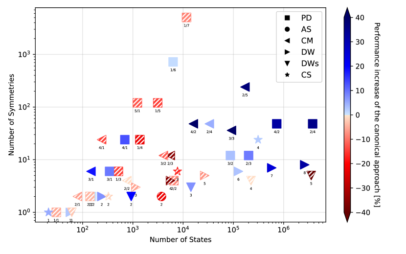
Figure 6: Comparing the percentage performance gain of the canonical and the membership approach with respect to the number of states and symmetries of the input problem for the benchmark families Package Delivery (PD), Alarm System (AS), CM, DW, DWs, CS. Labels are the parameters of the benchmark. A blue (unhatched) marker indicates a performance increase when using canonical representations.

In Fig. 6 we have plotted the instances of all benchmark families according to their number of symmetries and states. The color of the marker shows the percentaged in- or decrease in performance when using canonical representations while solving high-level Petri games. Blue (unhatched) indicates a performance gain when using the canonical approach. This shows that the benchmarks in general benefit from the canonical approach for an increasing number of states (the right blue (unhatched) area). However, the DWs benchmark (a simplified version of DW) exhibits the opposite behavior. This is most likely explained by the very simple structure, which favors a quick member check.

The algorithms are integrated in AdamSYNT [20, 21], open source, and available online. Additionally, we created an artifact with the current version running in a virtual machine for reproducing and checking all experimental data with provided scripts [19].

6 Related Work

For the synthesis of distributed systems other approaches are most prominently the Pnueli/Rosner model [22] and Zielonka’s asynchronous automata [23]. The synchronous setting of Pnueli/Rosner is in general undecidable [22], but some interesting architectures exist that have a decision procedure with nonelementary complexity [24, 25, 26]. For asynchronous automata, the decidability of the control problem is open in general, but again there are several interesting cases which have a decision procedure with nonelementary complexity [27, 28, 29].

Petri games based on P/T Petri nets are introduced in [5, 7]. Solving unbounded Petri games is in general undecidable. However, for Petri games with one environment player, a bounded number of system players, and a safety objective the problem is exptime-complete. The same complexity result holds for interchanged players [30]. High-level Petri games have been introduced in [9]. In [11], such Petri games are solved while exploiting symmetries. [31] gives outlooks towards high-level representations of strategies.

The symbolic Büchi game is inspired by the symbolic reachability graph for high-level nets from [14], and the calculation of canonical representatives [17] from [32]. There are several works on how to obtain symmetries of different subclasses of high-level Petri nets efficiently [33, 17, 32, 34] and for efficiency improvements for systems with different degrees of symmetrical behavior [35, 36, 37].

7 Conclusions and Outlook

We presented a new construction for the synthesis of distributed systems modeled by high-level Petri games with one environment player, an arbitrary number of system players, and a safety objective. The main idea is the reduction to a symbolic two-player Büchi game, in which the nodes are equivalence classes of symmetric situations in the Petri game. This leads to a significant reduction of the state space. The novelty of this construction is to obtain the reduction by introducing canonical representations. To this end, a theoretically cheaper construction of the Büchi game can be obtained depending on the input system. Additionally, the representations now allow to skip the inflated generation of an explicit Büchi game strategy and to directly generate a Petri game strategy from the symbolic Büchi game strategy. Our implementation, applied on six structurally different benchmark families, shows in general a performance gain in favor of the canonical representatives for larger state spaces.

In future work, we plan to integrate the algorithms in AdamWEB [38], a web interface for the synthesis of distributed systems, to allow for an easy insight in the symbolic games and strategies. Furthermore, we want to continue our investigation on the benefits of canonical representations, e.g., to directly generate high-level representations of Petri game strategies that match the given high-level Petri game.

Appendix

Appendix A Strategies in Petri Games – Formal Definition

We formally define strategies in Petri games as subprocesses of the unfolding.

First, we define concurrency and conflicts in Petri nets. Consider a Petri net $\mathsf{N}=(\mathsf{P},\mathsf{T},\mathsf{F},\mathsf{M}_{\mathsf{0}})$ and two nodes $\mathsf{x},\mathsf{y}\in\mathsf{P}\cup\mathsf{T}$. We write $\mathsf{x}<\mathsf{y}$, and call $\mathsf{x}$ causal predecessor of $\mathsf{y}$, if $\mathsf{x}\mathsf{F}^{+}\mathsf{y}$. Additionally, we write $\mathsf{x}\leq\mathsf{y}$ if $\mathsf{x}<\mathsf{y}$ or $\mathsf{x}=\mathsf{y}$, and call $\mathsf{x}$ and $\mathsf{y}$ causally related if $\mathsf{x}\leq\mathsf{y}$ or $\mathsf{y}\leq\mathsf{x}$. The nodes $\mathsf{x}$ and $\mathsf{y}$ are said to be in conflict, denoted by $\mathsf{x}\sharp\mathsf{y}$, if $\exists\mathsf{p}\in\mathsf{P}\,\exists\mathsf{t_{1}}\neq\mathsf{t_{2}}\in\mathit{post}(p):\mathsf{t_{1}}\leq\mathsf{x}\land\mathsf{t_{2}}\leq\mathsf{y}$. Two nodes are called concurrent, if they are neither in conflict, nor causally related. A set $\mathsf{X}\subseteq\mathsf{P}\cup\mathsf{T}$ is called concurrent, if each two elements in $\mathsf{X}$ are concurrent.

$\mathsf{N}$ is called an occurrence net if: i) every place has at most one transition in its preset, i.e., $\forall\mathsf{p}\in\mathsf{P}:|\mathit{pre}(\mathsf{p})|\leq 1$; ii) no transition is in self conflict, i.e., $\forall{\mathsf{t}\in\mathsf{T}:}\neg(\mathsf{t}\sharp\mathsf{t})$; iii) no node is its own causal predecessor, i.e., $\forall\mathsf{x}\in\mathsf{P}\cup\mathsf{T}:{\neg(\mathsf{x}<\mathsf{x})}$; iv) the initial marking contains exactly the places with no transition in their preset, i.e., $\mathsf{M}_{\mathsf{0}}=\{\mathsf{p}\in\mathsf{P}\,|\,\mathit{pre}(\mathsf{p})=\emptyset\}$. An occurrence net is called a causal net if additionally v) from every place there is at most one outgoing transition, i.e., $\forall\mathsf{p}\in\mathsf{P}:|\mathit{post}(\mathsf{p})|\leq 1$.

For a superscripted net $\mathsf{N}^{x}$, we implicitly also equip its components with the superscript, i.e., $\mathsf{N}^{x}=(\mathsf{P}^{x},\mathsf{T}^{x},\mathsf{F}^{x},\mathsf{M}_{\mathsf{0}}^{x})$, as well as the corresponding pre- and postset function $\mathit{pre}^{x},\mathit{post}^{x}$. Let $\mathsf{N}$ and $\mathsf{N}^{\prime}$ be two Petri nets. A function $h:\mathsf{P}\cup\mathsf{T}\to\mathsf{P}^{\prime}\cup\mathsf{T}^{\prime}$ is called a Petri net homomorphism, if: i) it maps places and transitions in $\mathsf{N}$ into the corresponding sets in $\mathsf{N}^{\prime}$, i.e., $\forall\mathsf{p}\in\mathsf{P}:{h(\mathsf{p})\in\mathsf{P}^{\prime}}\land\forall{\mathsf{t}\in\mathsf{T}}:h(\mathsf{t})\in\mathsf{T}^{\prime}$; ii) it maps the pre- and postset correspondingly, i.e., $\forall{\mathsf{t}\in\mathsf{T}}:\mathit{pre}^{\prime}(h(\mathsf{t}))=h(\mathit{pre}(\mathsf{t}))\land\mathit{post}^{\prime}(h(\mathsf{t}))=h(\mathit{post}(\mathsf{t}))$. The homomorphism is called initial if additionally iii) it maps the initial marking of $\mathsf{N}$ to the initial marking of $\mathsf{N}^{\prime}$, i.e., $h(\mathsf{M}_{\mathsf{0}})=\mathsf{M}_{\mathsf{0}}^{\prime}$.

A(n initial) branching process $\beta=(\mathsf{N}^{U},\lambda^{U})$ of $\mathsf{N}$ consists of an occurrence net $\mathsf{N}^{U}$ and a(n initial) homomorphism $\lambda^{U}:\mathsf{P}^{U}\cup\mathsf{T}^{U}\to\mathsf{P}\cup\mathsf{T}$ that is injective on transitions with same preset, i.e., $\forall\mathsf{\mathsf{t_{1}}},\mathsf{t_{2}}\in\mathsf{T}^{U}:(\mathit{pre}^{U}(\mathsf{t_{1}})=\mathit{pre}^{U}(\mathsf{t_{2}})\land\lambda^{U}(\mathsf{t_{1}})=\lambda^{U}(\mathsf{t_{2}}))\Rightarrow\mathsf{t_{1}}=\mathsf{t_{2}}$. If $\beta_{R}=(\mathsf{N}^{R},\rho)$ is an initial branching process of $\mathsf{N}$ with a causal net $\mathsf{N}^{R}$, $\beta_{R}$ is called an initial (concurrent) run of $\mathsf{N}$. A run formalizes a single concurrent execution of the net. For two branching processes $\beta=(\mathsf{N}^{U},\lambda^{U})$ and $\beta^{\prime}=({\mathsf{N}^{V}},{\lambda^{V}})$ we call $\beta$ a subprocess of $\beta^{\prime}$, if i) $\mathsf{N}^{U}$ is a subnet of ${\mathsf{N}^{V}}$, i.e., $\mathsf{P}^{U}\subseteq{\mathsf{P}^{V}},\mathsf{T}^{U}\subseteq{\mathsf{T}^{V}},\mathsf{F}^{U}\subseteq{\mathsf{F}^{V}},\mathsf{M}_{\mathsf{0}}^{U}={\mathsf{M}_{\mathsf{0}}^{V}}$; ii) ${\lambda^{V}}$ acts on $\mathsf{P}^{U}\cup\mathsf{T}^{U}$ as $\lambda^{U}$ does, i.e., ${\lambda^{V}}|_{\mathsf{P}^{U}\cup\mathsf{T}^{U}}=\lambda^{U}$.

A branching process $\beta=(\mathsf{N}^{U},\lambda^{U})$ is called an unfolding of $\mathsf{N}$, if for every transition that can occur in the net, there is a transition in the unfolding with corresponding label, i.e., $\forall\mathsf{t}\in\mathsf{T}\,\forall X\subseteq\mathsf{P}^{U}:X\text{ concurrent}\land\mathit{pre}(\mathsf{t})=\lambda^{U}(X)\Rightarrow\exists\mathsf{t}^{U}\in\mathsf{T}^{U}:\lambda^{U}(\mathsf{t}^{U})=\mathsf{t}\land\mathit{pre}^{U}(\mathsf{t}^{U})=X$. The unfolding of a net is unique up to isomorphism. The unfolding of a Petri game $\mathsf{G}=(\mathsf{P}_{\mathsf{S}},\mathsf{P}_{\mathsf{E}},\mathsf{T},\mathsf{F},\mathsf{M}_{0},\mathsf{P}_{\mathsf{B}})$ with underlying net $\mathsf{N}$ is the unfolding of $\mathsf{N}$, where the distinction of system-, environment-, and bad places is lifted to the branching process: $\mathsf{P}_{\mathsf{S}}^{U}=\{\mathsf{p}\in\mathsf{P}^{U}\,|\,\lambda^{U}(\mathsf{p})\in\mathsf{P}_{\mathsf{S}}\}$, $\mathsf{P}_{\mathsf{E}}^{U}=\{\mathsf{p}\in\mathsf{P}^{U}\,|\,\lambda^{U}(\mathsf{p})\in\mathsf{P}_{\mathsf{E}}\}$, and $\mathsf{P}_{\mathsf{B}}^{U}=\{\mathsf{p}\in\mathsf{P}^{U}\,|\,{\lambda^{U}(\mathsf{p})\in\mathsf{P}_{\mathsf{B}}}\}$.

A strategy for the system players in $\mathsf{G}$ is a subprocess $\sigma=(\mathsf{N}^{\sigma},\lambda^{\sigma})$ of the unfolding of $\mathsf{G}$ satisfying the following conditions:
Justified refusal: If a transition is forbidden in the strategy, then a system player in its preset uniformly forbids all occurrences in the strategy, i.e., $\forall\mathsf{t}\in\mathsf{T}^{U}:({\mathsf{t}\notin\mathsf{T}^{\sigma}}\land\mathit{pre}^{U}(t)\subseteq\mathsf{P}^{\sigma})\Rightarrow(\exists\mathsf{p}\in\mathit{pre}^{U}(\mathsf{t})\cap\mathsf{P}_{\mathsf{S}}^{\sigma}\,\forall\mathsf{t^{\prime}}\in\mathit{post}^{U}(\mathsf{p}):\lambda^{U}(\mathsf{t^{\prime}})=\lambda^{U}(\mathsf{t})\Rightarrow\mathsf{t^{\prime}}\notin\mathsf{T}^{\sigma})$. This also implies that no pure environment transition is forbidden.
Determinism: In no reachable marking (cut) in the strategy does a system player allow two transitions in his postset that are both enabled, i.e., $\forall\mathsf{p}\in\mathsf{P}_{\mathsf{S}}^{\sigma}\ \forall\mathsf{M}\in\mathcal{R}(\mathsf{N}^{\sigma}):\mathsf{p}\in\mathsf{M}\Rightarrow\exists^{\leq 1}\mathsf{t}\in\mathit{post}^{\sigma}(\mathsf{p}):\mathsf{M}[\mathsf{t}\rangle$. The set $\mathcal{R}(\mathsf{N}^{\sigma})$ are all reachable markings in the strategy.
Deadlock freedom: Whenever the system can proceed in $\mathsf{G}$, the strategy must also give the possibility to continue, i.e., $\forall\mathsf{M}\in\mathcal{R}(\mathsf{N}^{\sigma}):(\exists\mathsf{t}\in\mathsf{T}^{U}:\mathsf{M}[\mathsf{t}\rangle)\Rightarrow{\exists\mathsf{t^{\prime}}\in\mathsf{T}^{\sigma}:\mathsf{M}[\mathsf{t^{\prime}}\rangle}$.

An initial concurrent run $\pi=(\mathsf{N}^{R},\rho)$ of the underlying net $\mathsf{N}$ of a Petri game $\mathsf{G}$ is called a play in $\mathsf{G}$. The play $\pi$ conforms to $\sigma$ if it is a subprocess of $\sigma$. The system players win $\pi$ if $\mathsf{P}_{\mathsf{B}}^{R}=\emptyset$, otherwise the environment players win $\pi$. The strategy $\sigma$ is called winning, if all plays that conform to $\sigma$ are won by the system players. This is equivalent to $\mathsf{P}_{\mathsf{B}}^{\sigma}=\emptyset$.

References

• [1] Gieseking M, Würdemann N. Canonical Representations for Direct Generation of Strategies in High-Level Petri Games. In: Proc. Petri Nets (ICATPN) 2021, LNCS12734. 2021 pp. 95–117. URL https://doi.org/10.1007/978-3-030-76983-3_6.
• [2] Church A. Applications of recursive arithmetic to the problem of circuit synthesis. In: Summaries of the Summer Institute of Symbolic Logic, volume 1. Cornell Univ., Ithaca, NY, 1957 pp. 3–50.
• [3] Bloem R, Galler SJ, Jobstmann B, Piterman N, Pnueli A, Weiglhofer M. Interactive presentation: Automatic hardware synthesis from specifications: a case study. In: Proc. DATE 2007. 2007 pp. 1188–1193. URL https://dl.acm.org/citation.cfm?id=1266622.
• [4] Kress-Gazit H, Fainekos GE, Pappas GJ. Temporal-Logic-Based Reactive Mission and Motion Planning. IEEE Trans. Robotics, 2009. 25(6):1370–1381. URL https://doi.org/10.1109/TRO.2009.2030225.
• [5] Finkbeiner B, Olderog E. Petri Games: Synthesis of Distributed Systems with Causal Memory. In: Proc. GandALF 2014, EPTCS161. 2014 pp. 217–230. URL https://doi.org/10.4204/EPTCS.161.19.
• [6] Reisig W. Petri Nets: An Introduction, volume 4 of EATCS Monographs on Theoretical Computer Science. Springer, 1985. ISBN 3-540-13723-8. URL https://doi.org/10.1007/978-3-642-69968-9.
• [7] Finkbeiner B, Olderog E. Petri games: Synthesis of distributed systems with causal memory. Inf. Comput., 2017. 253:181–203. URL https://doi.org/10.1016/j.ic.2016.07.006.
• [8] Jensen K. Coloured Petri Nets - Basic Concepts, Analysis Methods and Practical Use - Volume 1. EATCS Monographs on Theoretical Computer Science. Springer, 1992. ISBN 978-3-662-06291-3. URL https://doi.org/10.1007/978-3-662-06289-0.
• [9] Gieseking M, Olderog E. High-Level Representation of Benchmark Families for Petri Games. CoRR, 2019. URL http://arxiv.org/abs/1904.05621.
• [10] Starke PH. Reachability Analysis of Petri Nets Using Symmetries. Syst. Anal. Model. Simul., 1991. 8(4–5):293–303.
• [11] Gieseking M, Olderog E, Würdemann N. Solving high-level Petri games. Acta Inf., 2020. 57(3-5):591–626. URL https://doi.org/10.1007/s00236-020-00368-5.
• [12] Grädel E, Thomas W, Wilke T (eds.). Automata, Logics, and Infinite Games, LNCS2500. Springer, 2002. URL https://doi.org/10.1007/3-540-36387-4.
• [13] Clarke EM, Emerson EA, Jha S, Sistla AP. Symmetry Reductions in Model Checking. In: Proc. CAV 1998, LNCS1427. 1998 pp. 147–158. URL https://doi.org/10.1007/BFb0028741.
• [14] Chiola G, Dutheillet C, Franceschinis G, Haddad S. A Symbolic Reachability Graph for Coloured Petri Nets. Theor. Comput. Sci., 1997. 176(1-2):39–65. URL https://doi.org/10.1016/S0304-3975(96)00010-2.
• [15] Esparza J, Heljanko K. Unfoldings - A Partial-Order Approach to Model Checking. EATCS Monographs in Theoretical Computer Science. Springer, 2008. ISBN 978-3-540-77425-9. URL https://doi.org/10.1007/978-3-540-77426-6.
• [16] Chiola G, Dutheillet C, Franceschinis G, Haddad S. Stochastic well-formed colored nets and symmetric modeling applications. IEEE Transactions on Computers, 1993. 42(11):1343–1360. URL https://doi.org/10.1109/12.247838.
• [17] Chiola G, Dutheillet C, Franceschinis G, Haddad S. On Well-Formed Coloured Nets and Their Symbolic Reachability Graph. In: Jensen K, Rozenberg G (eds.), High-level Petri Nets: Theory and Application, pp. 373–396. Springer. ISBN 978-3-642-84524-6, 1991. URL https://doi.org/10.1007/978-3-642-84524-6_13.
• [18] Hillah L, Kordon F, Petrucci-Dauchy L, Trèves N. PN Standardisation: A Survey. In: Proc. FORTE 2006,, LNCS4229. 2006 pp. 307–322. URL https://doi.org/10.1007/11888116_23.
• [19] Gieseking M, Würdemann N. Artifact: Canonical Representations for Direct Generation of Strategies in High-level Petri Games. 2021. URL https://doi.org/10.6084/m9.figshare.13697845.
• [20] Finkbeiner B, Gieseking M, Olderog E. Adam: Causality-Based Synthesis of Distributed Systems. In: Proc. CAV 2015, Part I, LNCS9206. 2015 pp. 433–439. URL https://doi.org/10.1007/978-3-319-21690-4_25.
• [21] Finkbeiner B, Gieseking M, Hecking-Harbusch J, Olderog E. Symbolic vs. Bounded Synthesis for Petri Games. In: Proc. SYNT@CAV 2017. 2017 pp. 23–43. URL https://doi.org/10.4204/EPTCS.260.5.
• [22] Pnueli A, Rosner R. Distributed Reactive Systems Are Hard to Synthesize. In: Proc. FOCS. IEEE Computer Society Press, 1990 pp. 746–757. URL https://doi.org/10.1109/FSCS.1990.89597.
• [23] Zielonka W. Asynchronous Automata. In: Diekert V, Rozenberg G (eds.), The Book of Traces, pp. 205–247. World Scientific, 1995. URL https://doi.org/10.1142/9789814261456_0007.
• [24] Rosner R. Modular Synthesis of Reactive Systems. Ph.D. thesis, Weizmann Institute of Science, Rehovot, Israel, 1992.
• [25] Kupferman O, Vardi MY. Synthesizing Distributed Systems. In: Proc. LICS 2001. 2001 pp. 389–398. URL https://doi.org/10.1109/LICS.2001.932514.
• [26] Finkbeiner B, Schewe S. Uniform Distributed Synthesis. In: Proc. LICS 2005. 2005 pp. 321–330. URL https://doi.org/10.1109/LICS.2005.53.
• [27] Genest B, Gimbert H, Muscholl A, Walukiewicz I. Asynchronous Games over Tree Architectures. In: Proc. ICALP 2013, Part II, LNCS7966. 2013 pp. 275–286. URL https://doi.org/10.1007/978-3-642-39212-2_26.
• [28] Muscholl A, Walukiewicz I. Distributed Synthesis for Acyclic Architectures. In: Raman V, Suresh SP (eds.), Proc. FSTTCS 2014, LIPIcs29. 2014 pp. 639–651. URL https://doi.org/10.4230/LIPIcs.FSTTCS.2014.639.
• [29] Madhusudan P, Thiagarajan PS, Yang S. The MSO Theory of Connectedly Communicating Processes. In: Proc. FSTTCS 2005, LNCS3821. 2005 pp. 201–212. URL https://doi.org/10.1007/11590156_16.
• [30] Finkbeiner B, Gölz P. Synthesis in Distributed Environments. In: Proc. FSTTCS 2017. 2017 pp. 28:1–28:14. URL https://doi.org/10.4230/LIPIcs.FSTTCS.2017.28.
• [31] Würdemann N. Exploiting symmetries of high-level Petri games in distributed synthesis. it Inf. Technol., 2021. 63(5-6):321–331. URL https://doi.org/10.1515/itit-2021-0012.
• [32] Chiola G, Dutheillet C, Franceschinis G, Haddad S. Stochastic Well-Formed Colored Nets and Symmetric Modeling Applications. IEEE Trans. Computers, 1993. 42(11):1343–1360. URL https://doi.org/10.1109/12.247838.
• [33] Dutheillet C, Haddad S. Regular stochastic Petri nets. In: Proc. Petri Nets (ICATPN) 1990. 1989 pp. 186–209. URL https://doi.org/10.1007/3-540-53863-1_26.
• [34] Lindquist M. Parameterized Reachability Trees for Predicate/Transition Nets. In: Proc. Petri Nets (ICATPN) 1991. 1991 pp. 301–324. URL https://doi.org/10.1007/3-540-56689-9_49.
• [35] Haddad S, Ilié J, Taghelit M, Zouari B. Symbolic Reachability Graph and Partial Symmetries. In: Proc. Petri Nets (ICATPN) 1995. 1995 pp. 238–257. URL https://doi.org/10.1007/3-540-60029-9_43.
• [36] Baarir S, Haddad S, Ilié J. Exploiting partial symmetries in well-formed nets for the reachability and the linear time model checking problems. In: Proc. WODES 2004. 2004 pp. 219–224. URL https://doi.org/10.1016/S1474-6670(17)30749-8.
• [37] Bellettini C, Capra L. A Quotient Graph for Asymmetric Distributed Systems. In: Proc. MASCOTS 2004. 2004 pp. 560–568. URL https://doi.org/10.1109/MASCOT.2004.1348313.
• [38] Gieseking M, Hecking-Harbusch J, Yanich A. A Web Interface for Petri Nets with Transits and Petri Games. In: Proc. TACAS 2021, Part II, LNCS12652. 2021 pp. 381–388. URL https://doi.org/10.1007/978-3-030-72013-1_22.