Reliable Simulation of Quantum Channels

Abstract

The Quantum Reverse Shannon Theorem has been a milestone in quantum information theory. It states that asymptotically reliable simulation of a quantum channel, assisted by unlimited shared entanglement, requires a rate of classical communication equal to the channel’s entanglement-assisted classical capacity. Here, we study the optimal speed at which the performance of channel simulation can exponentially approach the perfect, when the blocklength increases. This is known as the reliability function. We have determined the exact formula of the reliability function when the classical communication cost is not too high—below a critical value. This enables us to obtain, for the first time, an operational interpretation to the channel’s sandwiched Rényi mutual information of order from 1 to 2, since our formula of the reliability function is expressed as a transform of this quantity. In the derivation, we have also obtained an achievability bound for the simulation of finite many copies of the channel, which is of realistic significance.

Introduction.—Any dynamical process in nature can be modeled as a quantum channel. The simulation of quantum channels is not only a fundamental problem in quantum communication Bennett et al. (2014); Berta et al. (2011); Bennett et al. (2002); Devetak (2006); Berta et al. (2013); Fang et al. (2020); Takagi et al. (2020); Cubitt et al. (2011); Duan and Winter (2015), but has also attracted broad interest in the topics of quantum thermodynamics Faist et al. (2019, 2021) as well as general quantum resource theory Gour and Scandolo (2020); Regula and Takagi (2021); Chitambar and Gour (2019). Dual to the ordinary scenario of distilling perfect resources from noisy channels, channel simulation is the problem of generating a noisy channel by making use of noiseless resources.

The celebrated Quantum Reverse Shannon Theorem Bennett et al. (2014) concerns the optimal simulation of a noisy quantum channel by using classical communication, when an unlimited amount of free shared entanglement is available. It states that for the asymptotically reliable simulation of a quantum channel $\mathcal{N}_{A\rightarrow B}$ from system $A$ to system $B$, an amount of classical communication equal to the channel’s entanglement-assisted classical capacity $C_{E}(\mathcal{N})$, is necessary and sufficient Bennett et al. (2014); Berta et al. (2011). The entanglement-assisted classical capacity, in turn, is given by the channel’s mutual information Bennett et al. (1999, 2002)

$$C_{E}(\mathcal{N})=I(\mathcal{N}):=\max_{\varphi_{RA}}I(R:B)_{{\operatorname{id}}_{R}\otimes\mathcal{N}_{A\rightarrow B}(\varphi_{RA})},$$

where the maximization is over all pure state $\varphi_{RA}$ on system $A$ and a reference system $R$, and $I(R:B)_{{\operatorname{id}}\otimes\mathcal{N}(\varphi_{RA})}=S(\varphi_{R})-S(N(\varphi_{RA}))+S(N(\varphi_{A}))$ is the mutual information of the bipartite state $N(\varphi_{RA})$ note1 . Here, $S(\rho)=-\operatorname{Tr}(\rho\log\rho)$ is the von Neumann entropy. Being one of the foundational components of quantum Shannon theory, the Quantum Reverse Shannon Theorem establishes that $C_{E}$ is the unique quantity to characterize reversible conversion of one channel to another assisted by free entanglement, and it has found applications in proving strong converse theorems Bennett et al. (2014), rate-distortion theorems Datta et al. (2012); Wilde et al. (2013), as well as results in network information theory Hsieh and Watanabe (2016).

While the Quantum Reverse Shannon Theorem proves that $I(\mathcal{N})$ is the sharp threshold above which asymptotically reliable simulation of $\mathcal{N}_{A\rightarrow B}$ is possible, it does not answer the question regarding how fast perfect simulation can be approached as the copy of channels grows. This is the goal pursued by the study of the reliability function, which characterizes the best rate of exponential convergence of the performance of an information processing task towards the perfect Gallager (1968). The study of the reliability functions in quantum information dates back to more than two decades ago Burnashev and Holevo (1998); Winter (1999); Holevo (2000), and progresses have been made ever since Dalai (2013); Hayashi (2015); Dalai and Winter (2017); Cheng et al. (2019, 2020); Dupuis (2021), accompanied by fruitful results on the strong converse exponents characterizing the speed at which quantum information tasks become the useless Koenig and Wehner (2009); Sharma and Warsi (2013); Wilde et al. (2014); Gupta and Wilde (2015); Cooney et al. (2016); Mosonyi and Ogawa (2017); Cheng et al. (2020). However, full characterization of the reliability functions of quantum information processing tasks is rare until quite recently Li et al. (2021); Li and Yao (2021).

In this letter, we answer the question of how fast reliable reverse Shannon simulation of a quantum channel $\mathcal{N}_{A\rightarrow B}$ can be achieved, when the rate of classical communication is above the channel’s mutual information $I(\mathcal{N})$. Our main result is an in-depth characterization of the reliability function. By deriving tight upper and lower bounds, we have determined the exact formula for the reliability function, when the classical communication cost is not too high—below a critical value $R_{\textrm{critical}}$. In particular, we have obtained an explicit achievability bound for the performance of simulating $\mathcal{N}_{A\rightarrow B}^{\otimes n}$ for a finite blocklength $n$, which is of realistic significance. These results are given in terms of the sandwiched Rényi divergence Müller-Lennert et al. (2013); Wilde et al. (2014)

$$D_{\alpha}(\rho\|\sigma):=\frac{1}{\alpha-1}\log\operatorname{Tr}\left(\sigma^{\frac{1-\alpha}{2\alpha}}\rho\sigma^{\frac{1-\alpha}{2\alpha}}\right)^{\alpha},$$

defined for quantum states $\rho$, $\sigma$ and a real number $\alpha>0$. More specifically, the channel’s sandwiched Rényi mutual information Gupta and Wilde (2015) defined as follows, will play a crucial role:

$$I_{\alpha}(\mathcal{N}):=\max_{\varphi_{RA}}I_{\alpha}(R:B)_{{\operatorname{id}}_{R}\otimes\mathcal{N}_{A\rightarrow B}(\varphi_{RA})},$$

where the maximization is over all pure state $\varphi_{RA}$, and $I_{\alpha}(R:B)_{\rho_{RB}}:=\min\limits_{\sigma_{B}}D_{\alpha}(\rho_{AB}\|\rho_{A}\otimes\sigma_{B})$ is the sandwiched Rényi mutual information of a bipartite state.

Reverse Shannon simulation of quantum channels.—A quantum channel $\mathcal{N}_{A\rightarrow B}$ is a completely positive and trace-preserving (CPTP) map that sends states on the input Hilbert space $\mathcal{H}_{A}$ to states on the output Hilbert space $\mathcal{H}_{B}$. It is convenient to use the Stinespring dilation, which tells that there is an environment system $E$ and an isometric map $U_{\mathcal{N}}^{A\rightarrow BE}:\mathcal{H}_{A}\rightarrow\mathcal{H}_{B}\otimes\mathcal{H}_{E}$ such that $\mathcal{N}(\rho)=\operatorname{Tr}_{E}U_{\mathcal{N}}(\rho)\equiv\operatorname{Tr}_{E}U_{\mathcal{N}}\rho U_{\mathcal{N}}^{*}$ for any input state $\rho_{A}$. We say that a CPTP map $\mathcal{M}_{A\rightarrow B}$ is a reverse Shannon simulation for $\mathcal{N}_{A\rightarrow B}$, if it consists of using a shared bipartite entangled state between the sender Alice and the receiver Bob, applying local operation at Alice’s side, sending $c$ classical bits from Alice to Bob, and at last applying local operation at Bob’s side. The performance of the simulation is measured by the purified distance $P(\mathcal{M},\mathcal{N}):=\max_{\varphi_{RA}}P({\operatorname{id}}_{R}\otimes\mathcal{M}(\varphi_{RA}),{\operatorname{id}}_{R}\otimes\mathcal{N}(\varphi_{RA}))$, where for any two states $\rho$ and $\sigma$, $P(\rho,\sigma):=\sqrt{1-F^{2}(\rho,\sigma)}$ with $F(\rho,\sigma)=\|\sqrt{\rho}\sqrt{\sigma}\|_{1}$ being the fidelity. We define the optimal performance of reverse Shannon simulation for $\mathcal{N}_{A\rightarrow B}$, under the constraint that the classical communication cost is upper bounded by $c$ bits, as

$$P^{\rm{sim}}(\mathcal{N},c):=\min_{\mathcal{M}\in\mathfrak{S}_{c}}P\left(\mathcal{M}_{A\rightarrow B},\mathcal{N}_{A\rightarrow B}\right),$$ (1)

where $\mathfrak{S}_{c}$ is the set of all simulation maps with at most $c$ bits of classical communication.

For $n$ copies of the channel $\mathcal{N}_{A\rightarrow B}$, the optimal performance $P^{\rm{sim}}(\mathcal{N}^{\otimes n},nr)$ is expected to decrease exponentially with $n$. The reliability function of the reverse Shannon simulation of $\mathcal{N}_{A\rightarrow B}$ is defined as the rate of such exponential decreasing:

$$E^{\rm{sim}}(\mathcal{N},r):=\liminf_{n\rightarrow\infty}\frac{-1}{n}\log P^{\rm{sim}}\left(\mathcal{N}^{\otimes n},nr\right).$$ (2)

Symmetrization and de Finetti reduction.—Naturally, a simulation channel for $\mathcal{N}_{A\rightarrow B}^{\otimes n}$ has input system $A^{n}\equiv A_{1}A_{2}...A_{n}$ and output system $B^{n}\equiv B_{1}B_{2}...B_{n}$. We say that a channel $\mathcal{M}_{A^{n}\rightarrow B^{n}}$ is symmetric if

$$\mathcal{M}_{A^{n}\rightarrow B^{n}}=W_{B^{n}}^{\pi^{-1}}\circ\mathcal{M}_{A^{n}\rightarrow B^{n}}\circ W_{A^{n}}^{\pi}$$

holds for any permutation $\pi$ from the symmetric group over a set of $n$ elements. Here $W_{A^{n}}^{\pi}$ ($W_{B^{n}}^{\pi}$) is the natural representation of $\pi$ on $\mathcal{H}_{A^{n}}$ ($\mathcal{H}_{B^{n}}$). To achieve the best performance, we can always symmetrize the simulation channel $\mathcal{M}_{A^{n}\rightarrow B^{n}}$ by randomly applying a permutation and its inverse, respectively before and after the action of $\mathcal{M}$. This does not cause any loss of performance, as the target channel $\mathcal{N}^{\otimes n}$ itself is symmetric (see Supplemental Material sm ). The common randomness needed in the symmetrization can be obtained by making measurements at both sides of some shared maximally entangled states.

Now, once the simulation process is restricted to be symmetric, the technique of de Finetti reduction Christandl et al. (2009) applies. It states that the simulation will be good for any input states as long as it is good for the particular input state $\zeta_{R_{n}A^{n}}$, which is the purification of

$$\zeta_{A^{n}}:=\int\rho_{A}^{\otimes n}\mathrm{d}\,\mu(\rho)$$

with $\mu(\cdot)$ the probability measure on the space of density operators on $\mathcal{H}_{A}$ induced by the Hilbert-Schmidt metric. An alternative understanding for $\mu(\cdot)$ is by introducing a purification system $\bar{R}\cong A$. Then $\mu(\rho)=\nu(\phi_{\bar{R}A}(\rho))$, where $\phi_{\bar{R}A}(\rho)$ is the purification of $\rho_{A}$ and $\nu(\cdot)$ is the uniform spherical probability measure satisfying $\nu(\phi)=\nu(u\phi u^{*})$ for any unitary operator $u$ on $\mathcal{H}_{\bar{R}A}$. Specifically, the de Finetti reduction Christandl et al. (2009), reformulated in terms of the purified distance in the Supplemental Material sm , states that for any two symmetric channels $\mathcal{M}_{A^{n}\rightarrow B^{n}}$ and $\mathcal{E}_{A^{n}\rightarrow B^{n}}$,

$$P\left(\mathcal{M},\mathcal{E}\right)\leq\sqrt{g_{n,|A|}}P\left(\mathcal{M}(\zeta_{R_{n}A^{n}}),\mathcal{E}(\zeta_{R_{n}A^{n}})\right),$$ (3)

where $g_{n,|A|}:=\tbinom{n+|A|^{2}-1}{n}\leq(n+1)^{|A|^{2}-1}$ and $|A|$ is the dimension of $A$.

Channel simulation with a fixed input.—In light of the above observations, we now consider the problem of channel simulation with a fixed input state. For this case, the quantum state splitting protocol provides us an explicit simulation scheme Abeyesinghe et al. (2009); Bennett et al. (2014); Berta et al. (2011). This is the reverse procedure of quantum state merging, which in turn is related to quantum information decoupling Abeyesinghe et al. (2009); Anshu et al. (2017); Majenz et al. (2017). Employing the catalytic version of quantum information decoupling and its induced state merging strategy of Anshu et al. (2017); Majenz et al. (2017), we derive the following bound based on the analysis of Li and Yao (2021).

Proposition 1

Let $\mathcal{N}_{A\rightarrow B}$ be a quantum channel. Fix the input state $\varphi_{RA}$ and let $\varphi_{RB}=\mathcal{N}(\varphi_{RA})$. For arbitrary $c>0$ and state $\sigma_{B}$, there is a reverse Shannon simulation $\mathcal{M}_{A\rightarrow B}$ for $\mathcal{N}_{A\rightarrow B}$ with $c$ bits of classical communication, such that for any $s\in(0,1]$,

$$P\big{(}\mathcal{M}(\varphi_{RA}),\mathcal{N}(\varphi_{RA})\big{)}$$

$$\leq \sqrt{\frac{v^{s}}{s}}\exp\Big{\{}-\frac{\ln 2}{2}s\big{(}c-D_{1+s}(\varphi_{RB}\|\varphi_{R}\otimes\sigma_{B})\big{)}\Big{\}},$$ (4)

where $v$ is the number of distinct eigenvalues of $\varphi_{R}\otimes\sigma_{B}$.

We describe briefly the construction of the simulation map that achieves the bound of Eq. (4). Suppose that a referee, Alice, and Bob share the state $\varphi_{R:E:B}={\operatorname{id}}_{R}\otimes U_{\mathcal{N}}^{A\rightarrow BE}(\varphi_{RA})$, where $U_{\mathcal{N}}$ is the Stinespring dilation of the channel $\mathcal{N}$. Here and in what follows the subscript separated by colons indicates that the systems from left to right are respectively held by the referee, Alice and Bob. As shown in Li and Yao (2021), there is a merging strategy that consists of Alice and Bob sharing a pair of entangled pure state $\gamma_{A^{\prime}B^{\prime}}$, Bob applying a unitary map $V_{BB^{\prime}\rightarrow B_{1}B_{2}}$ where $\log|B_{2}|=\frac{c}{2}$, Bob sending the $B_{2}$ system to Alice through a noiseless channel ${\operatorname{id}}_{B_{2}\rightarrow\bar{B}_{2}}$ with $B_{2}\cong\bar{B}_{2}$, and at last Alice applying another unitary map $W_{EA^{\prime}\bar{B}_{2}\rightarrow BEA_{1}}$, such that the resulting state $\Psi_{R:BEA_{1}:B_{1}}=W\circ{\operatorname{id}}_{B_{2}\rightarrow\bar{B}_{2}}\circ V(\varphi_{R:E:B}\otimes\gamma_{\emptyset:A^{\prime}:B^{\prime}})$ satisfies

$$P(\Psi_{R:BEA_{1}:B_{1}},\varphi_{R:BE:\emptyset}\otimes\omega_{\emptyset:A_{1}:B_{1}})$$

$$\leq \sqrt{\frac{v^{s}}{s}}\exp\Big{\{}-\frac{\ln 2}{2}s\big{(}c-D_{1+s}(\varphi_{RB}\|\varphi_{R}\otimes\sigma_{B})\big{)}\Big{\}}.$$

Here $\emptyset$ represents an empty set of systems and $\omega_{A_{1}B_{1}}$ is a pure entangled state shared between Alice and Bob. Now, for the input state $\varphi_{RA}$, the simulation of $\mathcal{N}_{A\rightarrow B}$ consists of: (a) Alice and Bob sharing the entangled state $\omega_{A_{1}B_{1}}$ for assistance, (b) Alice applying the Stinespring dilation $U_{\mathcal{N}}^{A\rightarrow BE}$ locally, (c) Alice applying $W^{-1}$, (d) Alice implementing the noiseless transmission ${\operatorname{id}}_{{\bar{B}}_{2}\rightarrow B_{2}}$ to Bob via quantum teleportation Bennett et al. (1993), which consumes $c$ bits of classical communication, (e) Bob applying $V^{-1}$. The resulting state is denoted as $\Phi_{R:EA^{\prime}:BB^{\prime}}$. Because these simulation steps unitarily reverse the merging procedure, we have

$$\begin{split}&P(\Phi_{R:EA^{\prime}:BB^{\prime}},\varphi_{R:E:B}\otimes\gamma_{\emptyset:A^{\prime}:B^{\prime}})\\ =&P(\Psi_{R:BEA_{1}:B_{1}},\varphi_{R:BE:\emptyset}\otimes\omega_{\emptyset:A_{1}:B_{1}}).\end{split}$$

At last, discarding the systems $E$, $A^{\prime}$ and $B^{\prime}$, we obtain the simulation which achieves the claimed bound.

Achievability.—Our first main result is the following achievability bound for the simulation of $\mathcal{N}_{A\rightarrow B}^{\otimes n}$ for any finite $n$.

Theorem 2

Let $\mathcal{N}_{A\rightarrow B}$ be a quantum channel. For the reverse Shannon simulation of $\mathcal{N}_{A\rightarrow B}^{\otimes n}$ with bounded classical communication rate $r>0$, we have

$$P^{\rm{sim}}\left(\mathcal{N}^{\otimes n},nr\right)\leq f(n,s)\exp{\Big{\{}\!-n\frac{\ln 2}{2}s\big{(}r-I_{1+s}(\mathcal{N})\big{)}\Big{\}}},$$

where $s\in(0,1]$ is arbitrary, and we set $f(n,s)=\sqrt{s^{-1}(n+1)^{(1+s)(d+1)^{2}}}$ with $d:=\max\{|A|,|B|\}$.

We sketch the argument for Theorem 2. At first, we apply Proposition 1 to the channel $\mathcal{N}_{A\rightarrow B}^{\otimes n}$ with input state $\zeta_{R_{n}A^{n}}$. Let $\zeta_{R_{n}B^{n}}=\mathcal{N}^{\otimes n}(\zeta_{R_{n}A^{n}})$. We fix an $s\in(0,1]$ and pick $\sigma^{*}_{B^{n}}$ to be the state that is symmetric and minimizes $D_{1+s}(\zeta_{R_{n}B^{n}}\|\zeta_{R_{n}}\otimes\sigma_{B^{n}})$. Then Proposition 1 tells us that there is a reverse Shannon simulation ${\mathcal{M}}_{A^{n}\rightarrow B^{n}}$ with $nr$ bits of classical communication, such that

$$P\left({\mathcal{M}}(\zeta_{R_{n}A^{n}}),\mathcal{N}^{\otimes n}(\zeta_{R_{n}A^{n}})\right)$$

$$\leq \sqrt{\frac{v_{n}^{s}}{s}}\exp\Big{\{}-\frac{\ln 2}{2}s\big{(}nr-I_{1+s}(R_{n}:B^{n})_{\zeta_{R_{n}B^{n}}}\big{)}\Big{\}},$$ (5)

where $v_{n}\leq(n+1)^{(d+2)(d-1)}$ is the number of distinct eigenvalues of $\zeta_{R_{n}}\otimes\sigma^{*}_{B^{n}}$. The map $\mathcal{M}_{A^{n}\rightarrow B^{n}}$ can be assumed to be symmetric. Otherwise, a symmetrization makes it so and this is without loss of performance, as both $\zeta_{A^{n}}$ and $\mathcal{N}_{A\rightarrow B}^{\otimes n}$ are symmetric. At this stage, the de Finetti reduction of Eq. (3) applies, letting us obtain

$$P^{\rm{sim}}\left(\mathcal{N}^{\otimes n},nr\right)\leq P\left(\mathcal{M},\mathcal{N}^{\otimes n}\right)$$

$$\leq \sqrt{g_{n,d}}\ P\left({\mathcal{M}}(\zeta_{R_{n}A^{n}}),\mathcal{N}^{\otimes n}(\zeta_{R_{n}A^{n}})\right).$$ (6)

The last step is to employ the additivity property established in Gupta and Wilde (2015): $I_{\alpha}(\mathcal{E}_{1}\otimes\mathcal{E}_{2})=I_{\alpha}(\mathcal{E}_{1})+I_{\alpha}(\mathcal{E}_{2})$ for any channels $\mathcal{E}_{1}$, $\mathcal{E}_{2}$ and $\alpha\geq 1$. This leads to

$$I_{1+s}(R_{n}:B^{n})_{\zeta_{R_{n}B^{n}}}\leq I_{1+s}(\mathcal{N}^{\otimes n})=nI_{1+s}(\mathcal{N}).$$ (7)

The combination of Eqs. (5)–(7) completes the argument.

Converse.—For $\lambda>0$, the smoothing quantity for the max-information of a bipartite quantum state $\rho_{RB}$, denoted by $\delta_{R:B}(\rho_{RB},\lambda)$, is defined Li and Yao (2021) as

$$\min\left\{P(\tilde{\rho}_{RB},\rho_{RB}):\tilde{\rho}_{RB}\leq 2^{\lambda}\rho_{R}\otimes\sigma_{B}\right\},$$ (8)

where $\tilde{\rho}_{RB}$ and $\sigma_{B}$ run over all quantum states. Employing this quantity, we derive the following one-shot converse bound.

Theorem 3

Let $\mathcal{N}_{A\rightarrow B}$ be a quantum channel and $c>0$. For any bipartite pure state $\varphi_{RA}$ we have

$$P^{\rm{sim}}(\mathcal{N},c)\geq\delta_{R:B}\big{(}\mathcal{N}(\varphi_{RA}),c\big{)}.$$ (9)

A short proof is as follows. Since the optimal simulation performance is evaluated for the worst case over all the input states, we can lower bound it using an arbitrary input state $\varphi_{RA}$. That is,

$$P^{\rm{sim}}(\mathcal{N},c)\geq\min_{\mathcal{M}\in\mathfrak{S}_{c}}P\big{(}\mathcal{M}(\varphi_{RA}),\mathcal{N}(\varphi_{RA})\big{)},$$ (10)

where $\mathfrak{S}_{c}$ is the set of all the simulation maps for $\mathcal{N}_{A\rightarrow B}$ whose classical communication cost does not exceed $c$ bits. Fix $\mathcal{M}_{A\rightarrow B}\in\mathfrak{S}_{c}$. It consists of (a) using a shared bipartite entangled state $\omega_{A_{1}B_{1}}$ for assistance, (b) applying local operation $\mathcal{E}_{AA_{1}\rightarrow X}$ with $\log|X|\leq c$ at Alice’s side, (c) sending $X$ from Alice to Bob via a noiseless classical channel $\overline{{\operatorname{id}}}_{X\rightarrow X}:\ \rho_{X}\mapsto\sum_{x}\langle x|\rho_{X}|x\rangle|x\rangle\!\langle x|_{X}$ with $\{|x\rangle\}_{x}$ a standard basis of $\mathcal{H}_{X}$, (d) applying local operation $\mathcal{D}_{XB_{1}\rightarrow B}$ at Bob’s side. The crucial idea is to consider the state

$$\Phi_{RXB_{1}}:=\overline{{\operatorname{id}}}_{X\rightarrow X}\circ\mathcal{E}_{AA_{1}\rightarrow X}(\varphi_{RA}\otimes\omega_{A_{1}B_{1}})$$

shared by the referee ($R$) and Bob ($XB_{1}$), after the simulation steps (a), (b) and (c) being performed. The fact that $\Phi_{RXB_{1}}$ is classical in $X$ ensures that

$$\Phi_{RXB_{1}}\leq 2^{c}\varphi_{R}\otimes\big{(}\frac{{\openone}_{X}}{|X|}\otimes\omega_{B_{1}}\big{)}.$$

Then applying the CPTP map $\mathcal{D}_{XB_{1}\rightarrow B}$ at both sides, we get

$$\mathcal{M}_{A\rightarrow B}(\varphi_{RA})\leq 2^{c}\varphi_{R}\otimes\mathcal{D}_{XB_{1}\rightarrow B}\big{(}\frac{{\openone}_{X}}{|X|}\otimes\omega_{B_{1}}\big{)},$$

which, according to Eq. (8), implies

$$P\big{(}\mathcal{M}(\varphi_{RA}),\mathcal{N}(\varphi_{RA})\big{)}\geq\delta_{R:B}\big{(}\mathcal{N}(\varphi_{RA}),c\big{)}.$$ (11)

Combining Eq. (10) and Eq. (11) finishes the proof.

Reliability function.—Now we study the reliability function. As defined in Eq. (2), this is the optimal exponent under which the simulation of $\mathcal{N}_{A\rightarrow B}^{\otimes n}$ approaches the perfect, as $n\rightarrow\infty$. Building on Theorem 2 and Theorem 3, we derive the following in-depth characterization of the reliability function.

Theorem 4

Let $\mathcal{N}_{A\rightarrow B}$ be a quantum channel and $r\geq 0$. The reliability function $E^{\rm{sim}}(\mathcal{N},r)$ for the reverse Shannon simulation of $\mathcal{N}_{A\rightarrow B}$ satisfies

$$E^{\rm{sim}}(\mathcal{N},r) \geq\frac{1}{2}\max_{0\leq s\leq 1}\big{\{}s\big{(}r-I_{1+s}(\mathcal{N})\big{)}\big{\}},$$ (12)

$$E^{\rm{sim}}(\mathcal{N},r) \leq\frac{1}{2}\sup_{s\geq 0}\big{\{}s\big{(}r-I_{1+s}(\mathcal{N})\big{)}\big{\}}.$$ (13)

In particular, when $r\leq R_{\rm{critical}}:=\frac{\mathrm{d}}{\mathrm{d}s}sI_{1+s}(\mathcal{N})\big{|}_{s=1}$,

$$E^{\rm{sim}}(\mathcal{N},r)=\frac{1}{2}\max_{0\leq s\leq 1}\big{\{}s\big{(}r-I_{1+s}(\mathcal{N})\big{)}\big{\}}.$$ (14)

Eq. (12) is a result of Theorem 2, and Eq. (13) follows from Theorem 3 by an application of the exact exponent for smoothing the max-information of Ref. Li and Yao (2021). Eq. (14) holds because when $r\leq R_{\textrm{critical}}$, the lower bound of Eq. (12) and the upper bound of Eq. (13) coincide. See the Supplemental Material sm for the proof.

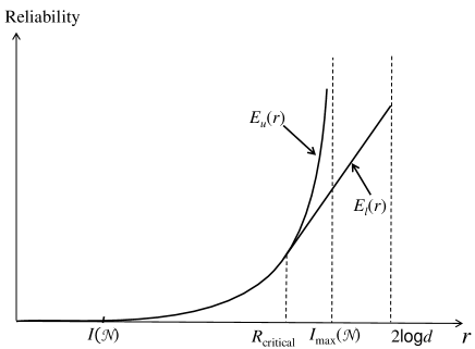
Figure 1: Reliability function of quantum channel simulation. $E_{l}(r):=\frac{1}{2}\max_{0\leq s\leq 1}\big{\{}s\big{(}r-I_{1+s}(\mathcal{N})\big{)}\big{\}}$ is the lower bound of Eq. (12). $E_{u}(r):=\frac{1}{2}\sup_{s\geq 0}\big{\{}s\big{(}r-I_{1+s}(\mathcal{N})\big{)}\big{\}}$ is the upper bound of Eq. (13). The two bounds are equal in the interval $[0,R_{\text{critical}}]$, giving the exact reliability function. Above the critical value $R_{\text{critical}}$, the upper bound $E_{u}(r)$ increases faster and it diverges to infinity when $r>I_{\text{max}}(\mathcal{N}):=\lim\limits_{\alpha\rightarrow\infty}I_{\alpha}(\mathcal{N})$, while the lower bound $E_{l}(r)$ becomes linear and reaches $\log d-\frac{1}{2}I_{2}(\mathcal{N})$ at $r=2\log d$ with $d:=\min\{|A|,|B|\}$.

The results of Theorem 4 are depicted in Fig. 1. As long as the classical communication rate $r$ is below the critical value $R_{\text{critical}}$, we have determined the explicit formula for the reliability function. When the classical communication rate $r$ is above the critical value, the two fundamental bounds diverge from each other more and more. It is worth pointing out that when $r\geq 2\log\min\{|A|,|B|\}$, perfect simulation can be achieved by teleportation Bennett et al. (1993), even in the one-shot setting. So in this situation the reliability function is infinity.

The case around the channel’s mutual information $I(\mathcal{N})$ is of particular interest. We will see that the Quantum Reverse Shannon Theorem follows as an immediate corollary of Theorem 4.

Corollary 5

Quantum Reverse Shannon Theorem Bennett et al. (2014); Berta et al. (2011): for a quantum channel $\mathcal{N}_{A\rightarrow B}$, the minimum classical communication rate $C_{\rm{QRST}}$ needed for the asymptotically reliable simulation of $\mathcal{N}_{A\rightarrow B}$ is given by the channel’s mutual information $I(\mathcal{N})$.

Proof. It is shown in Cooney et al. (2016) that $I_{1+s}(\mathcal{N})$ is an increasing function of $s$ and $I_{1+s}(\mathcal{N})$ converges to $I(\mathcal{N})$ as $s$ goes to $0$. With this we get from Theorem 4 that $E^{\rm{sim}}(\mathcal{N},r)=0$ when $r\leq I(\mathcal{N})$, and $E^{\rm{sim}}(\mathcal{N},r)>0$ when $r>I(\mathcal{N})$. The latter implies that any rate $r$ above $I(\mathcal{N})$ is sufficient for asymptotically reliable simulation. So, $C_{\rm{QRST}}\leq I(\mathcal{N})$. On the other hand, $C_{\rm{QRST}}\geq I(\mathcal{N})$ is obvious Bennett et al. (2014); Berta et al. (2011), because the rate of classical communication necessary for reliable simulation of $\mathcal{N}_{A\rightarrow B}$ has to be at least equal to the channel’s entanglement-assisted classical capacity, which is $I(\mathcal{N})$ Bennett et al. (2002).     $\sqcap$$\sqcup$

Conclusion.—We have derived fundamental achievability and converse bounds for the performance of reverse Shannon simulation of a quantum channel. These bounds translate to the corresponding lower and upper bounds for the reliability function. By showing that the lower bound and upper bound coincide when the classical communication rate $r$ is such that $r\leq R_{\textrm{critical}}$, we have obtained the exact formula of the reliability function for $r$ falling in this range. Remarkably, our result has provided, for the first time, an operational interpretation to the channel’s sandwiched Rényi mutual information of order from 1 to 2.

It is well known that with the assistance of free entanglement, two bits of classical communication is equivalent to one qubit of quantum communication, as the consequence of quantum teleportation Bennett et al. (1993) and dense coding Bennett and Wiesner (1992). Thus our solution applies as well to the problem of channel simulation with quantum communication assisted by unlimited free entanglement.

When the classical communication rate is above the critical point, we are unable to obtain the reliability function. In fact, the existence of a critical point, of which at one side the problem remains unsolved, is a common phenomenon in the study of reliability functions Gallager (1968); Dalai (2013); Li et al. (2021). Works in literature (e.g., Shannon (1956); Gallager (1968); Lovász (1979)) suggest that combinatorics may come into play. We leave it as an open problem. We note that an independent work RTB2021moderate has obtained the moderate deviation expansion for reverse Shannon simulation of quantum channels. The second-order asymptotics of this task remains a major open problem. Yet another interesting problem related to our work, is to find the reliability function for entanglement-assisted communication over quantum channels.

Acknowledgements.—The research of KL was supported by NSFC (No. 61871156, No. 12031004), and the research of YY was supported by NSFC (No. 61871156, No. 12071099).

Supplemental Material

In this Supplemental Material, we include all the proofs in full detail.

1. Notation and preliminaries

Let $\mathcal{H}$ be a Hilbert space. $\mathcal{P}(\mathcal{H})$ denotes the set of positive semidefinite operators on $\mathcal{H}$. The set of density operators is denoted as $\mathcal{S}(\mathcal{H})$, and the set of subnormalized density operators is denoted as $\mathcal{S}_{\leq}(\mathcal{H})$. When $\mathcal{H}$ is associated with a system $X$, the notations $\mathcal{P}(X)$, $\mathcal{S}(X)$ and $\mathcal{S}_{\leq}(X)$ are used for $\mathcal{P}(\mathcal{H})$, $\mathcal{S}(\mathcal{H})$ and $\mathcal{S}_{\leq}(\mathcal{H})$, respectively. For a pure state $|\varphi\rangle$, the corresponding density operator $|\varphi\rangle\!\langle\varphi|$ is abbreviated as $\varphi$. The purified distance between two channels $\mathcal{M}_{A\rightarrow B}$ and $\mathcal{N}_{A\rightarrow B}$ is defined as

$$P\left(\mathcal{M}_{A\rightarrow B},\mathcal{N}_{A\rightarrow B}\right):=\max_{\varphi_{RA}}P\left({\operatorname{id}}_{R}\otimes\mathcal{M}(\varphi_{RA}),{\operatorname{id}}_{R}\otimes\mathcal{N}(\varphi_{RA})\right),$$

where for two states $\rho$ and $\sigma$, the purified distance is given by $P(\rho,\sigma)=\sqrt{1-F^{2}(\rho,\sigma)}$ with $F(\rho,\sigma)=\|\sqrt{\rho}\sqrt{\sigma}\|_{1}$ being the fidelity. For a unitary operation $U$, $U(\rho)$ is the abbreviation of $U\rho U^{*}$. For every $n\in\mathbb{N}$, let $S_{n}$ denote the symmetric group over the set $\{1,2,\ldots,n\}$. For a Hilbert space $\mathcal{H}_{A}$ and a permutation $\pi\in S_{n}$, the natural representation of $\pi$ is the unitary operator $W^{\pi}_{A^{n}}$ on $\mathcal{H}_{A}^{\otimes n}$, given by

$$W^{\pi}_{A^{n}}:|\psi_{1}\rangle\otimes\cdots\otimes|\psi_{n}\rangle\mapsto|\psi_{\pi^{-1}(1)}\rangle\otimes\cdots\otimes|\psi_{\pi^{-1}(n)}\rangle,\quad\forall\ |\psi_{i}\rangle\in\mathcal{H}_{A}.$$

The symmetric subspace of $\mathcal{H}_{A}^{\otimes n}$ is denoted as $\mathrm{Sym}(\mathcal{H}_{A}^{\otimes n})$, which is the linear space consists of all vectors $|v\rangle\in\mathcal{H}_{A}^{\otimes n}$ satisfying the permutation-invariant property

$$|v\rangle=W^{\pi}_{A^{n}}|v\rangle,\quad\forall\ \pi\in S_{n}.$$

2. Formulation of the problem

The quantum reverse Shannon simulation concerns how to use classical communication and unlimited entanglement to simulate any quantum channel $\mathcal{N}_{A\rightarrow B}$.

Definition 6

Let $\mathcal{N}_{A\rightarrow B}$ be a quantum channel from Alice to Bob. A CPTP map $\mathcal{M}_{A\rightarrow B}$ is a reverse Shannon simulation for $\mathcal{N}_{A\rightarrow B}$ if it consists of using a shared bipartite entangled state, applying local operation at Alice’s side, sending $c$ classical bits from Alice to Bob, and at last applying local operation at Bob’s side. The performance of the simulation is measured by the purified distance between the two channels $P(\mathcal{M}_{A\rightarrow B},\mathcal{N}_{A\rightarrow B})$.

We define the optimal performance of reverse Shannon simulation under the constraint that the classical communication cost is limited.

Definition 7

Let $\mathcal{N}_{A\rightarrow B}$ be a quantum channel. For given $c\geq 0$, the optimal performance of reverse Shannon simulation for $\mathcal{N}_{A\rightarrow B}$, given that the classical communication cost is upper bounded by $c$ bits, is defined as

$$P^{\rm{sim}}(\mathcal{N}_{A\rightarrow B},c):=\min_{\mathcal{M}_{A\rightarrow B}\in\mathfrak{S}_{c}}P(\mathcal{M}_{A\rightarrow B},\mathcal{N}_{A\rightarrow B}),$$ (15)

where $\mathfrak{S}_{c}$ is the set of all the reverse Shannon simulations for $\mathcal{N}_{A\rightarrow B}$ whose classical communication cost does not exceed $c$ bits.

Now, we are ready to introduce the reliability function.

Definition 8

Let $\mathcal{N}_{A\rightarrow B}$ be a quantum channel. For given $r\geq 0$, the reliability function $E^{\rm{sim}}(\mathcal{N}_{A\rightarrow B},r)$ of the reverse Shannon simulation of $\mathcal{N}_{A\rightarrow B}$ is defined as

$$E^{\rm{sim}}(\mathcal{N}_{A\rightarrow B},r):=\liminf_{n\rightarrow\infty}\frac{-1}{n}\log P^{\rm{sim}}\big{(}\mathcal{N}^{\otimes n}_{A\rightarrow B},nr\big{)}.$$ (16)

In fact, we can also use quantum communication and unlimited entanglement to simulate the channel $\mathcal{N}_{A\rightarrow B}$. This is called reverse Shannon simulation via quantum communication.

Definition 9

Let $\mathcal{N}_{A\rightarrow B}$ be a quantum channel from Alice to Bob. A reverse Shannon simulation via quantum communication for $\mathcal{N}_{A\rightarrow B}$ consists of using a shared bipartite entangled state $\phi_{A^{\prime}B^{\prime}}$, applying unitary transformation $U_{AA^{\prime}\rightarrow M\tilde{A}}$ at Alice’s side, sending the system $M$ from Alice to Bob, and at last applying unitary transformation $V_{B^{\prime}M\rightarrow B\tilde{B}}$ at Bob’s side. The simulation map is given by

$$\mathcal{M}_{A\rightarrow B}(\cdot):=\operatorname{Tr}_{\tilde{A}\tilde{B}}\Big{[}V_{B^{\prime}M\rightarrow B\tilde{B}}U_{AA^{\prime}\rightarrow M\tilde{A}}\big{(}(\cdot)\otimes\phi_{A^{\prime}B^{\prime}}\big{)}\Big{]}.$$ (17)

The performance of the simulation is measured by the purified distance between the two channels $P(\mathcal{M}_{A\rightarrow B},\mathcal{N}_{A\rightarrow B})$.

Similarly, we define the optimal performance under the constraint that the quantum communication cost is bounded.

Definition 10

Let $\mathcal{N}_{A\rightarrow B}$ be a quantum channel. For given $c\geq 0$, the optimal performance of reverse Shannon simulation via quantum communication for $\mathcal{N}_{A\rightarrow B}$, given that the quantum communication cost is upper bounded by $c$ qubits, is defined as

$$P_{q}^{\rm{sim}}(\mathcal{N}_{A\rightarrow B},c):=\min_{\mathcal{M}_{A\rightarrow B}\in\mathfrak{Q}_{c}}P(\mathcal{M}_{A\rightarrow B},\mathcal{N}_{A\rightarrow B}),$$ (18)

where $\mathfrak{Q}_{c}$ is the set of all the reverse Shannon simulations for $\mathcal{N}_{A\rightarrow B}$ with quantum communication not more than $c$ qubits.

The following relation is a direct result of the teleportation and dense coding protocols Bennett et al. (1993); Bennett and Wiesner (1992).

Lemma 11

Let $\mathcal{N}_{A\rightarrow B}$ be a quantum channel. For any $c\geq 0$ we have

$$P^{\rm{sim}}(\mathcal{N}_{A\rightarrow B},2c)=P_{q}^{\rm{sim}}(\mathcal{N}_{A\rightarrow B},c).$$

3. Symmetrizing the simulation channel

We show that to optimize the performance, the simulation channel can always be chosen to be symmetric.

Lemma 12

Given the channel $\mathcal{N}_{A\rightarrow B}$ and a simulation channel $\mathcal{M}_{A^{n}\rightarrow B^{n}}$ for $\mathcal{N}_{A\rightarrow B}^{\otimes n}$, we let

$$\widetilde{\mathcal{M}}_{A^{n}\rightarrow B^{n}}=\sum_{\pi\in S_{n}}\frac{1}{|S_{n}|}W_{B^{n}}^{\pi^{-1}}\circ\mathcal{M}_{A^{n}\rightarrow B^{n}}\circ W_{A^{n}}^{\pi}$$ (19)

be the symmetrization of $\mathcal{M}_{A^{n}\rightarrow B^{n}}$. Then

$$P\big{(}\widetilde{\mathcal{M}}_{A^{n}\rightarrow B^{n}},\mathcal{N}_{A\rightarrow B}^{\otimes n}\big{)}\leq P\big{(}\mathcal{M}_{A^{n}\rightarrow B^{n}},\mathcal{N}_{A\rightarrow B}^{\otimes n}\big{)}.$$

Proof. For any pure state $\varphi_{RA^{n}}$, we have

$$F\big{(}\widetilde{\mathcal{M}}(\varphi_{RA^{n}}),\mathcal{N}^{\otimes n}(\varphi_{RA^{n}})\big{)}$$

$$= F\Big{(}\sum_{\pi\in S_{n}}\frac{1}{|S_{n}|}W_{B^{n}}^{\pi^{-1}}\circ\mathcal{M}\circ W_{A^{n}}^{\pi}(\varphi_{RA^{n}}),\sum_{\pi\in S_{n}}\frac{1}{|S_{n}|}W_{B^{n}}^{\pi^{-1}}\circ\mathcal{N}^{\otimes n}\circ W_{A^{n}}^{\pi}(\varphi_{RA^{n}})\Big{)}$$

$$\geq \sum_{\pi\in S_{n}}\frac{1}{|S_{n}|}F\big{(}W_{B^{n}}^{\pi^{-1}}\circ\mathcal{M}\circ W_{A^{n}}^{\pi}(\varphi_{RA^{n}}),W_{B^{n}}^{\pi^{-1}}\circ\mathcal{N}^{\otimes n}\circ W_{A^{n}}^{\pi}(\varphi_{RA^{n}})\big{)}$$

$$= \sum_{\pi\in S_{n}}\frac{1}{|S_{n}|}F\big{(}\mathcal{M}(W_{A^{n}}^{\pi}(\varphi_{RA^{n}})),\mathcal{N}^{\otimes n}(W_{A^{n}}^{\pi}(\varphi_{RA^{n}}))\big{)}$$

$$\geq \sum_{\pi\in S_{n}}\frac{1}{|S_{n}|}\min_{\varphi^{\prime}_{RA^{n}}}F\big{(}\mathcal{M}(\varphi^{\prime}_{RA^{n}}),\mathcal{N}^{\otimes n}(\varphi^{\prime}_{RA^{n}})\big{)}$$

$$= \min_{\varphi^{\prime}_{RA^{n}}}F\big{(}\mathcal{M}(\varphi^{\prime}_{RA^{n}}),\mathcal{N}^{\otimes n}(\varphi^{\prime}_{RA^{n}})\big{)},$$

where the second line is due to the fact that $\mathcal{N}_{A\rightarrow B}^{\otimes n}$ is symmetric, and the third line follows from the joint concavity of the fidelity Watrous (2018). This is equivalent to

$$\begin{split}P\big{(}\widetilde{\mathcal{M}}(\varphi_{RA^{n}}),\mathcal{N}^{\otimes n}(\varphi_{RA^{n}})\big{)}\leq&\max_{\varphi^{\prime}_{RA^{n}}}P\big{(}\mathcal{M}(\varphi^{\prime}_{RA^{n}}),\mathcal{N}^{\otimes n}(\varphi^{\prime}_{RA^{n}})\big{)}\\ =&P\big{(}\mathcal{M}_{A^{n}\rightarrow B^{n}},\mathcal{N}_{A\rightarrow B}^{\otimes n}\big{)}.\end{split}$$

As $\varphi_{RA^{n}}$ is chosen arbitrarily, the statement follows.      $\sqcap$$\sqcup$

4. de Finetti reduction

The de Finetti reduction, also known as post-selection technique, was proved in Christandl et al. (2009) using the completely bounded trace norm as the measure for distance between quantum channels. Here we reformulate this result by employing the purified distance. For completeness, we give a proof, which follows the same idea as the original proof of Christandl et al. (2009), though. We point out that this reformulation based on the purified distance is made independently in RTB2021moderate as well.

Lemma 13

Let $\mathcal{M}_{A^{n}\rightarrow B^{n}}$ and $\mathcal{E}_{A^{n}\rightarrow B^{n}}$ be symmetric channels such that $\mathcal{M}=W_{B^{n}}^{\pi^{-1}}\circ\mathcal{M}\circ W_{A^{n}}^{\pi}$ and $\mathcal{E}=W_{B^{n}}^{\pi^{-1}}\circ\mathcal{E}\circ W_{A^{n}}^{\pi}$ for any permutation $\pi\in S_{n}$. Let $\zeta_{\tilde{R}\bar{R}^{n}A^{n}}$ be the purification of the maximally mixed state supported on the symmetric subspace of $\mathcal{H}_{\bar{R}A}^{\otimes n}$, where $\bar{R}\cong A$. That is,

$$\zeta_{\bar{R}^{n}A^{n}}=\int\phi_{\bar{R}A}^{\otimes n}\mathrm{d}\nu(\phi_{\bar{R}A}),$$

where the integration is over all pure states on $\mathcal{H}_{\bar{R}A}$ and $\nu(\cdot)$ is the unique uniform spherical measure satisfying $\nu(\phi)=\nu(u\phi u^{*})$ for any unitary transformation $u$ on $\mathcal{H}_{\bar{R}A}$. Set $g_{n,|A|}:=\tbinom{n+|A|^{2}-1}{n}\leq(n+1)^{|A|^{2}-1}$. We have

$$P(\mathcal{M}_{A^{n}\rightarrow B^{n}},\mathcal{E}_{A^{n}\rightarrow B^{n}})\leq\sqrt{g_{n,|A|}}\ P\big{(}\mathcal{M}(\zeta_{\tilde{R}\bar{R}^{n}A^{n}}),\mathcal{E}(\zeta_{\tilde{R}\bar{R}^{n}A^{n}})\big{)}.$$

Note that the state $\zeta_{R_{n}A^{n}}$ in the main paper is identical to $\zeta_{\tilde{R}\bar{R}^{n}A^{n}}$ by setting $R_{n}\equiv\tilde{R}\bar{R}^{n}$.

Proof. We start with an arbitrary state $\varphi_{TA^{n}}$ in which $T$ is any reference system. Set

$$\tilde{\varphi}_{GTA^{n}}:=\frac{1}{|S_{n}|}\sum_{\pi\in S_{n}}|\pi\rangle\!\langle\pi|_{G}\otimes({\operatorname{id}}_{T}\otimes W^{\pi}_{A^{n}})(\varphi_{TA^{n}}).$$

Then $\tilde{\varphi}_{A^{n}}$ is invariant under permutations. So it has a symmetric purification $\tilde{\varphi}_{\bar{R}^{n}A^{n}}$, which can be written in the vector form as

$$|\tilde{\varphi}\rangle_{\bar{R}^{n}A^{n}}=\sqrt{(|A|)^{n}}\big{(}{\openone}_{\bar{R}^{n}}\otimes\sqrt{\tilde{\varphi}_{A^{n}}}\big{)}(|\Phi\rangle_{\bar{R}A})^{\otimes n}\in\mathrm{Sym}(\mathcal{H}_{\bar{R}A}^{\otimes n}),$$

where $|\Phi\rangle_{\bar{R}A}=\frac{1}{\sqrt{|A|}}\sum_{i=1}^{|A|}|i\rangle_{\bar{R}}|i\rangle_{A}$ is the maximally entangled state. We have

$$1-F\big{(}\mathcal{M}(\varphi_{TA^{n}}),\mathcal{E}(\varphi_{TA^{n}})\big{)}$$

$$= 1-\sum_{\pi\in S_{n}}\frac{1}{|S_{n}|}F\big{(}\mathcal{M}(W^{\pi}_{A^{n}}(\varphi_{TA^{n}})),\mathcal{E}(W^{\pi}_{A^{n}}(\varphi_{TA^{n}}))\big{)}$$

$$= 1-F\big{(}\mathcal{M}(\tilde{\varphi}_{GTA^{n}}),\mathcal{E}(\tilde{\varphi}_{GTA^{n}})\big{)}$$

$$\leq 1-F\big{(}\mathcal{M}(\tilde{\varphi}_{\bar{R}^{n}A^{n}}),\mathcal{E}(\tilde{\varphi}_{\bar{R}^{n}A^{n}})\big{)},$$ (20)

where the second line is due to the symmetry of $\mathcal{M}_{A^{n}\rightarrow B^{n}}$ and $\mathcal{E}_{A^{n}\rightarrow B^{n}}$ as well as the fact that the fidelity function is invariant under the action of unitary operations, the third line is by direct calculation, and the last line follows from the monotonicity of the fidelity function under CPTP maps.

Let $\{|\tilde{\varphi}^{(a)}\rangle_{\bar{R}^{n}A^{n}}\}_{a=1}^{g_{n,|A|}}$ be an orthonormal basis of $\mathrm{Sym}(\mathcal{H}_{\bar{R}A}^{\otimes n})$, with the identification $|\tilde{\varphi}^{(1)}\rangle_{\bar{R}^{n}A^{n}}\equiv|\tilde{\varphi}\rangle_{\bar{R}^{n}A^{n}}$. Note that the dimension of $\mathrm{Sym}(\mathcal{H}_{\bar{R}A}^{\otimes n})$ is exactly $g_{n,|A|}$. Then $\zeta_{\bar{R}^{n}A^{n}}=\frac{1}{g_{n,|A|}}\sum_{a=1}^{g_{n,|A|}}\tilde{\varphi}^{(a)}_{\bar{R}^{n}A^{n}}$ and we can write

$$|\zeta\rangle_{\tilde{R}\bar{R}^{n}A^{n}}=\frac{1}{\sqrt{g_{n,|A|}}}\sum_{a=1}^{g_{n,|A|}}|a\rangle_{\tilde{R}}|\tilde{\varphi}^{(a)}\rangle_{\bar{R}^{n}A^{n}},$$

where $\{|a\rangle_{\tilde{R}}\}$ is an orthonormal basis of $\tilde{R}$. We now have

$$F\big{(}\mathcal{M}(\zeta_{\tilde{R}\bar{R}^{n}A^{n}}),\mathcal{E}(\zeta_{\tilde{R}\bar{R}^{n}A^{n}})\big{)}$$

$$\leq F\Big{(}\mathcal{M}\big{(}\frac{1}{{g_{n,|A|}}}\sum_{a}|a\rangle\!\langle a|_{\tilde{R}}\otimes\tilde{\varphi}^{(a)}_{\bar{R}^{n}A^{n}}\big{)},\mathcal{E}\big{(}\frac{1}{{g_{n,|A|}}}\sum_{a}|a\rangle\!\langle a|_{\tilde{R}}\otimes\tilde{\varphi}^{(a)}_{\bar{R}^{n}A^{n}}\big{)}\Big{)}$$

$$= \frac{1}{{g_{n,|A|}}}F\big{(}\mathcal{M}(\tilde{\varphi}_{\bar{R}^{n}A^{n}}),\mathcal{E}(\tilde{\varphi}_{\bar{R}^{n}A^{n}})\big{)}+\frac{1}{{g_{n,|A|}}}\sum_{a=2}^{g_{n,|A|}}F\big{(}\mathcal{M}(\tilde{\varphi}_{\bar{R}^{n}A^{n}}^{(a)}),\mathcal{E}(\tilde{\varphi}_{\bar{R}^{n}A^{n}}^{(a)})\big{)}$$

$$\leq \frac{1}{{g_{n,|A|}}}F\big{(}\mathcal{M}(\tilde{\varphi}_{\bar{R}^{n}A^{n}}),\mathcal{E}(\tilde{\varphi}_{\bar{R}^{n}A^{n}})\big{)}+\frac{g_{n,|A|}-1}{g_{n,|A|}},$$ (21)

where the first inequality comes from the monotonicity of the fidelity function under CPTP maps.

From Eq. (20) and Eq. (21) we get that

$$g_{n,|A|}\Big{(}1-F\big{(}\mathcal{M}(\zeta_{\tilde{R}\bar{R}^{n}A^{n}}),\mathcal{E}(\zeta_{\tilde{R}\bar{R}^{n}A^{n}})\big{)}\Big{)}$$

$$\geq 1-F\big{(}\mathcal{M}(\tilde{\varphi}_{\bar{R}^{n}A^{n}}),\mathcal{E}(\tilde{\varphi}_{\bar{R}^{n}A^{n}})\big{)}$$

$$\geq 1-F\big{(}\mathcal{M}(\varphi_{TA^{n}}),\mathcal{E}(\varphi_{TA^{n}})\big{)}.$$

Since the state $\varphi_{TA^{n}}$ was chosen arbitrarily, the above relation lets us obtain

$$P(\mathcal{M}_{A^{n}\rightarrow B^{n}},\mathcal{E}_{A^{n}\rightarrow B^{n}})$$

$$= \sqrt{1-\min_{\varphi_{TA^{n}}}F\big{(}\mathcal{M}(\varphi_{TA^{n}}),\mathcal{E}(\varphi_{TA^{n}})\big{)}^{2}}$$

$$\leq \sqrt{\Big{(}1-\min_{\varphi_{TA^{n}}}F\big{(}\mathcal{M}(\varphi_{TA^{n}}),\mathcal{E}(\varphi_{TA^{n}})\big{)}\Big{)}\Big{(}1+F\big{(}\mathcal{M}(\zeta_{\tilde{R}\bar{R}^{n}A^{n}}),\mathcal{E}(\zeta_{\tilde{R}\bar{R}^{n}A^{n}})\big{)}\Big{)}}$$

$$\leq \sqrt{g_{n,|A|}\Big{(}1-F\big{(}\mathcal{M}(\zeta_{\tilde{R}\bar{R}^{n}A^{n}}),\mathcal{E}(\zeta_{\tilde{R}\bar{R}^{n}A^{n}})\big{)}\Big{)}\Big{(}1+F\big{(}\mathcal{M}(\zeta_{\tilde{R}\bar{R}^{n}A^{n}}),\mathcal{E}(\zeta_{\tilde{R}\bar{R}^{n}A^{n}})\big{)}\Big{)}}$$

$$= \sqrt{g_{n,|A|}}\ P\big{(}\mathcal{M}(\zeta_{\tilde{R}\bar{R}^{n}A^{n}}),\mathcal{E}(\zeta_{\tilde{R}\bar{R}^{n}A^{n}})\big{)},$$

completing the proof.      $\sqcap$$\sqcup$

5. Channel simulation with a fixed input state

This section contains a detailed proof of Proposition 1.

Proof of Proposition 1. Let $U_{\mathcal{N}}^{A\rightarrow BE}$ be the Stinespring dilation of the channel $\mathcal{N}_{A\rightarrow B}$. We start with an introduction of quantum state merging with respect to the state $\varphi_{REB}={\operatorname{id}}_{R}\otimes U_{\mathcal{N}}^{A\rightarrow BE}(\varphi_{RA})$. Suppose that $\varphi_{REB}$ is held by a referee ($R$), Alice ($E$), and Bob ($B$). This is compactly represented by $\varphi_{R:E:B}$. That is, when multiple systems are separated by two colons, it means that the three parts from left to right are respectively held by the referee, Alice and Bob. Based on the protocol introduced in Majenz et al. (2017); Anshu et al. (2017), a tight achievability bound has been derived in Li and Yao (2021), for merging the $B$ part of $\varphi_{R:E:B}$ to Alice. The merging scheme consists of the following steps:

1. Alice and Bob share a pair of entangled pure state $\gamma_{A^{\prime}B^{\prime}}$ (here $\gamma_{A^{\prime}B^{\prime}}$ depends on $\sigma_{B}$, and it can be denoted as $\gamma_{\emptyset:A^{\prime}:B^{\prime}}$, where $\emptyset$ stands for an empty set of systems);

2. Bob applies a local unitary transformation $V_{BB^{\prime}\rightarrow B_{1}B_{2}}$, where the size of the the $B_{2}$ system is $\log|B_{2}|=\frac{c}{2}$;

3. Bob sends the $B_{2}$ system to Alice via the noiseless channel ${\operatorname{id}}_{B_{2}\rightarrow\bar{B}_{2}}$ with $B_{2}\cong\bar{B}_{2}$;

4. Alice applies a local unitary transformation $W_{EA^{\prime}\bar{B}_{2}\rightarrow BEA_{1}}$.

Write the resulting state as $\Psi_{R:BEA_{1}:B_{1}}=W\circ{\operatorname{id}}_{B_{2}\rightarrow\bar{B}_{2}}\circ V(\varphi_{R:E:B}\otimes\gamma_{\emptyset:A^{\prime}:B^{\prime}})$. Then there exists a pure entangled state $\omega_{A_{1}B_{1}}$ shared between Alice and Bob, such that (Li and Yao, 2021, Theorem 7 and Proposition 11)

$$P(\Psi_{R:BEA_{1}:B_{1}},\varphi_{R:BE:\emptyset}\otimes\omega_{\emptyset:A_{1}:B_{1}})\leq\sqrt{\frac{v^{s}}{s}}\exp\Big{\{}-\frac{\ln 2}{2}s\big{(}c-D_{1+s}(\varphi_{RB}\|\varphi_{R}\otimes\sigma_{B})\big{)}\Big{\}},$$ (22)

where $s$ and $v$ are as specified in the statement of the proposition.

Now, for the input state $\varphi_{RA}$, the reverse Shannon simulation for $\mathcal{N}_{A\rightarrow B}$ is constructed essentially by reversing the above steps (this is called state splitting):

1. Alice and Bob share the entangled state $\omega_{A_{1}B_{1}}$ for assistance;

2. Alice applies the Stinespring dilation $U_{\mathcal{N}}^{A\rightarrow BE}$ locally (now the whole state is $\varphi_{R:BE:\emptyset}\otimes\omega_{\emptyset:A_{1}:B_{1}}$);

3. Alice applies the unitary transformation $W^{-1}$;

4. Alice implements the noiseless transmission ${\operatorname{id}}_{{\bar{B}}_{2}\rightarrow B_{2}}$ to Bob via quantum teleportation, which consumes $c$ bits of classical communication;

5. Bob applies the unitary transformation $V^{-1}$.

We denote the resulting state as $\Phi_{R:EA^{\prime}:BB^{\prime}}$. Then

$$\Phi_{R:EA^{\prime}:BB^{\prime}}=V^{-1}\circ{\operatorname{id}}_{\bar{B}_{2}\rightarrow B_{2}}\circ W^{-1}(\varphi_{R:BE:\emptyset}\otimes\omega_{\emptyset:A_{1}:B_{1}}),$$

and we have

$$P\big{(}\Phi_{R:EA^{\prime}:BB^{\prime}},\varphi_{R:E:B}\otimes\gamma_{\emptyset:A^{\prime}:B^{\prime}}\big{)}$$

$$= P\big{(}V^{-1}\circ{\operatorname{id}}_{\bar{B}_{2}\rightarrow B_{2}}\circ W^{-1}(\varphi_{R:BE:\emptyset}\otimes\omega_{\emptyset:A_{1}:B_{1}}),\varphi_{R:E:B}\otimes\gamma_{\emptyset:A^{\prime}:B^{\prime}}\big{)}$$

$$= P\big{(}\varphi_{R:BE:\emptyset}\otimes\omega_{\emptyset:A_{1}:B_{1}},W\circ{\operatorname{id}}_{B_{2}\rightarrow\bar{B}_{2}}\circ V(\varphi_{R:E:B}\otimes\gamma_{\emptyset:A^{\prime}:B^{\prime}}\big{)}$$

$$= P\big{(}\Psi_{R:BEA_{1}:B_{1}},\varphi_{R:BE:\emptyset}\otimes\omega_{\emptyset:A_{1}:B_{1}}\big{)},$$ (23)

where for the third line we apply the unitary operation $W\circ{\operatorname{id}}_{B_{2}\rightarrow\bar{B}_{2}}\circ V$ to both states, and for the fourth line we exchange the position of the two states. At last, the simulation map $\mathcal{M}_{A\rightarrow B}$ is obtained by discarding the systems $E$, $A^{\prime}$ and $B^{\prime}$ after the above steps (a)-(e). Thus,

$$\mathcal{M}_{A\rightarrow B}(\varphi_{RA})=\operatorname{Tr}_{EA^{\prime}B^{\prime}}[\Phi_{R:EA^{\prime}:BB^{\prime}}].$$

So, we have

$$P\big{(}\mathcal{M}(\varphi_{RA}),\mathcal{N}(\varphi_{RA})\big{)}$$

$$= P\big{(}\operatorname{Tr}_{EA^{\prime}B^{\prime}}[\Phi_{R:EA^{\prime}:BB^{\prime}}],\varphi_{R:\emptyset:B}\big{)}$$

$$\leq P\big{(}\Phi_{R:EA^{\prime}:BB^{\prime}},\varphi_{R:E:B}\otimes\gamma_{\emptyset:A^{\prime}:B^{\prime}}\big{)}$$

$$\leq \sqrt{\frac{v^{s}}{s}}\exp\Big{\{}-\frac{\ln 2}{2}s\big{(}c-D_{1+s}(\varphi_{RB}\|\varphi_{R}\otimes\sigma_{B})\big{)}\Big{\}},$$

where the third line is by the monotonicity of purified distance under partial trace, and the last line comes from the combination of Eq. (22) and Eq. (23).      $\sqcap$$\sqcup$

6. Achievability bound

This section contains a detailed proof of Theorem 2.

Proof of Theorem 2. Since we can always symmetrize the simulation channel, according to the de Finetti reduction (Lemma 13), it suffices to consider the special input state $\zeta_{R_{n}A^{n}}$. Let $\zeta_{R_{n}B^{n}}=\mathcal{N}_{A\rightarrow B}^{\otimes n}(\zeta_{R_{n}A^{n}})$. From now on, we fix an $s\in(0,1]$. As shown in Lemma 14, we can choose a symmetric (permutation-invariant) state $\sigma^{*}_{B^{n}}$ to minimize $D_{1+s}(\zeta_{R_{n}B^{n}}\|\zeta_{R_{n}}\otimes\sigma_{B^{n}})$, such that

$$D_{1+s}(\zeta_{R_{n}B^{n}}\|\zeta_{R_{n}}\otimes\sigma^{*}_{B^{n}})=I_{1+s}(R_{n}:B^{n})_{\mathcal{N}_{A\rightarrow B}^{\otimes n}(\zeta_{R_{n}A^{n}})}.$$ (24)

Denote the number of distinct eigenvalues of a quantum state $\rho$ as $|\operatorname{spec}(\rho)|$, where $\operatorname{spec}(\cdot)$ stands for the spectral set. For a symmetric state $\rho_{X^{n}}$, $|\operatorname{spec}(\rho_{X^{n}})|$ is polynomial in $n$, upper bounded by the sum of the dimensions of all the irreducible decompositions of the representation $u\mapsto u^{\otimes n}$ of the unitary group on $\mathcal{H}_{X}^{\otimes n}$. An explicit bound of $(n+1)^{\frac{(|X|+2)(|X|-1)}{2}}$ can be found in, e.g., Hayashi2010universal . So, we have

$$|\operatorname{spec}(\zeta_{R_{n}}\otimes\sigma^{*}_{B^{n}})|\leq|\operatorname{spec}(\zeta_{A^{n}})|\cdot|\operatorname{spec}(\sigma^{*}_{B^{n}})|\leq(n+1)^{(d+2)(d-1)},$$ (25)

where $d:=\max\{|A|,|B|\}$, and for the first inequality we have used $|\operatorname{spec}(\zeta_{R_{n}})|=|\operatorname{spec}(\zeta_{A^{n}})|$ since $\zeta_{R_{n}A^{n}}$ is a pure state.

Now, we apply Proposition 1 to the channel $\mathcal{N}_{A\rightarrow B}^{\otimes n}$ with the fixed input state $\zeta_{R_{n}A^{n}}$. Set $c=nr$ and $\sigma_{B^{n}}=\sigma^{*}_{B^{n}}$. According to Proposition 1, there is a reverse Shannon simulation ${\mathcal{M}^{\prime}}_{A^{n}\rightarrow B^{n}}$ with $c=nr$ bits of classical communication, such that for $s$ fixed earlier,

$$P\left({\mathcal{M}^{\prime}}_{A^{n}\rightarrow B^{n}}(\zeta_{R_{n}A^{n}}),\mathcal{N}_{A\rightarrow B}^{\otimes n}(\zeta_{R_{n}A^{n}})\right)$$

$$\leq \sqrt{\frac{(n+1)^{(d+2)(d-1)s}}{s}}\exp\Big{\{}-\frac{\ln 2}{2}s\big{(}nr-D_{1+s}(\zeta_{R_{n}B^{n}}\|\zeta_{R_{n}}\otimes\sigma^{*}_{B^{n}})\big{)}\Big{\}}$$

$$= \sqrt{\frac{(n+1)^{(d+2)(d-1)s}}{s}}\exp\Big{\{}-\frac{\ln 2}{2}s\big{(}nr-I_{1+s}(R_{n}:B^{n})_{\mathcal{N}_{A\rightarrow B}^{\otimes n}(\zeta_{R_{n}A^{n}})}\big{)}\Big{\}},$$ (26)

where the equality is by Eq. (24). Next, we symmetrize ${\mathcal{M}^{\prime}}_{A^{n}\rightarrow B^{n}}$ to obtain a symmetric simulation $\mathcal{M}_{A^{n}\rightarrow B^{n}}$. This is the final simulation scheme that we need. The symmetrization consumes some classical randomness which can be obtained by making measurements on the shared entanglement. Meanwhile, it does not cause loss of performance, because

$$P\left({\mathcal{M}}_{A^{n}\rightarrow B^{n}}(\zeta_{R_{n}A^{n}}),\mathcal{N}_{A\rightarrow B}^{\otimes n}(\zeta_{R_{n}A^{n}})\right)$$

$$= P\Big{(}\sum_{\pi\in S_{n}}\frac{1}{|S_{n}|}W_{B^{n}}^{\pi^{-1}}\circ{\mathcal{M}^{\prime}}_{A^{n}\rightarrow B^{n}}\circ W_{A^{n}}^{\pi}(\zeta_{R_{n}A^{n}}),\mathcal{N}_{A\rightarrow B}^{\otimes n}(\zeta_{R_{n}A^{n}})\Big{)}$$

$$\leq \max_{\pi\in S_{n}}P\left(W_{B^{n}}^{\pi^{-1}}\circ{\mathcal{M}^{\prime}}_{A^{n}\rightarrow B^{n}}\circ W_{A^{n}}^{\pi}(\zeta_{R_{n}A^{n}}),\mathcal{N}_{A\rightarrow B}^{\otimes n}(\zeta_{R_{n}A^{n}})\right)$$

$$= P\left({\mathcal{M}^{\prime}}_{A^{n}\rightarrow B^{n}}(\zeta_{R_{n}A^{n}}),\mathcal{N}_{A\rightarrow B}^{\otimes n}(\zeta_{R_{n}A^{n}})\right),$$ (27)

where the third line follows from the concavity of the fidelity together with the definition of purified distance, and the last line is because both $\zeta_{A^{n}}$ and $\mathcal{N}_{A\rightarrow B}^{\otimes n}$ are invariant under permutation and we also use a trick of Eq. (32). At this stage, we are ready to apply the de Finetti reduction (Lemma 13) to get

$$P^{\rm{sim}}\left(\mathcal{N}^{\otimes n},nr\right)\leq P\left({\mathcal{M}}_{A^{n}\rightarrow B^{n}},\mathcal{N}_{A\rightarrow B}^{\otimes n}\right)$$

$$\leq \sqrt{g_{n,|A|}}P\left({\mathcal{M}}_{A^{n}\rightarrow B^{n}}(\zeta_{R_{n}A^{n}}),\mathcal{N}_{A\rightarrow B}^{\otimes n}(\zeta_{R_{n}A^{n}})\right).$$ (28)

Combining Eqs. (26)–(28), we arrive at

$$P^{\rm{sim}}\left(\mathcal{N}^{\otimes n},nr\right)\leq\sqrt{\frac{(n+1)^{(1+s)(d+1)^{2}}}{s}}\exp\Big{\{}-\frac{\ln 2}{2}s\big{(}nr-I_{1+s}(R_{n}:B^{n})_{\mathcal{N}_{A\rightarrow B}^{\otimes n}(\zeta_{R_{n}A^{n}})}\big{)}\Big{\}}.$$ (29)

Eq. (29) holds for any $s\in(0,1]$, because it was chosen arbitrarily at the beginning of the proof.

The last step is to employ the additivity property of the channel’s sandwiched Rényi mutual information established in Gupta and Wilde (2015): for $\alpha\geq 1$ and any two channels $\mathcal{E}_{1}$ and $\mathcal{E}_{2}$, $I_{\alpha}(\mathcal{E}_{1}\otimes\mathcal{E}_{2})=I_{\alpha}(\mathcal{E}_{1})+I_{\alpha}(\mathcal{E}_{2})$. This yields

$$I_{1+s}(R_{n}:B^{n})_{\mathcal{N}_{A\rightarrow B}^{\otimes n}(\zeta_{R_{n}A^{n}})}\leq I_{1+s}(\mathcal{N}_{A\rightarrow B}^{\otimes n})=nI_{1+s}(\mathcal{N}_{A\rightarrow B}).$$ (30)

Inserting Eq. (30) into Eq. (29) lets us complete the proof.      $\sqcap$$\sqcup$

Lemma 14

For the quantum state $\zeta_{R_{n}B^{n}}=\mathcal{N}_{A\rightarrow B}^{\otimes n}(\zeta_{R_{n}A^{n}})$ and for $s\geq-\frac{1}{2}$, let $\sigma^{*}_{B^{n}}$ be a minimizer of

$$\min_{\sigma_{B^{n}}}D_{1+s}(\zeta_{R_{n}B^{n}}\|\zeta_{R_{n}}\otimes\sigma_{B^{n}})=I_{1+s}(R_{n}:B^{n})_{\mathcal{N}_{A\rightarrow B}^{\otimes n}(\zeta_{R_{n}A^{n}})}.$$

Then $\sigma^{*}_{B^{n}}$ can be chosen to be symmetric, i.e., $\sigma^{*}_{B^{n}}=W^{\pi}_{B^{n}}(\sigma^{*}_{B^{n}})$ for all $\pi\in S_{n}$.

Proof. For any state $\sigma_{B^{n}}$, we have

$$D_{1+s}\left(\zeta_{R_{n}B^{n}}\|\zeta_{R_{n}}\otimes\sigma_{B^{n}}\right)$$

$$= D_{1+s}\left(W^{\pi}_{B^{n}}\circ\mathcal{N}_{A\rightarrow B}^{\otimes n}(\zeta_{R_{n}A^{n}})\|\zeta_{R_{n}}\otimes W^{\pi}_{B^{n}}(\sigma_{B^{n}})\right)$$

$$= D_{1+s}\left(\mathcal{N}_{A\rightarrow B}^{\otimes n}\circ W^{\pi}_{A^{n}}(\zeta_{R_{n}A^{n}})\|\zeta_{R_{n}}\otimes W^{\pi}_{B^{n}}(\sigma_{B^{n}})\right),$$ (31)

where the second line is because the sandwiched Rényi divergence is invariant under unitary operations, and the third line is due to the fact that $\mathcal{N}_{A\rightarrow B}^{\otimes n}=W^{-\pi}_{B^{n}}\circ\mathcal{N}_{A\rightarrow B}^{\otimes n}\circ W^{\pi}_{A^{n}}$. Because $\zeta_{A^{n}}$ is semmetric, the pure states $W^{\pi}_{A^{n}}(\zeta_{R_{n}A^{n}})$ and $\zeta_{R_{n}A^{n}}$ are identical on the $A^{n}$ system. So, by Uhlmann’s theorem Uhlmann1976transition , there is a unitary operation $V_{R_{n}}$ such that

$$W^{\pi}_{A^{n}}(\zeta_{R_{n}A^{n}})=V_{R_{n}}(\zeta_{R_{n}A^{n}}).$$ (32)

Eq. (32) ensures that we also have $\zeta_{R_{n}}=V_{R_{n}}(\zeta_{R_{n}})$. Inserting these two relations into Eq. (31), we obtain

$$D_{1+s}\left(\zeta_{R_{n}B^{n}}\|\zeta_{R_{n}}\otimes\sigma_{B^{n}}\right)$$

$$= D_{1+s}\big{(}V_{R_{n}}(\zeta_{R_{n}B^{n}})\|V_{R_{n}}(\zeta_{R_{n}})\otimes W^{\pi}_{B^{n}}(\sigma_{B^{n}})\big{)}$$

$$= D_{1+s}\big{(}\zeta_{R_{n}B^{n}}\|\zeta_{R_{n}}\otimes W^{\pi}_{B^{n}}(\sigma_{B^{n}})\big{)}.$$ (33)

Let $\tilde{\sigma}_{B^{n}}=\sum_{\pi\in S_{n}}\frac{1}{|S_{n}|}W^{\pi}_{B^{n}}(\sigma_{B^{n}})$ be the symmetrization of $\sigma_{B^{n}}$. Then

$$D_{1+s}\left(\zeta_{R_{n}B^{n}}\|\zeta_{R_{n}}\otimes\tilde{\sigma}_{B^{n}}\right)$$

$$\leq \sum_{\pi\in S_{n}}\frac{1}{|S_{n}|}D_{1+s}\big{(}\zeta_{R_{n}B^{n}}\|\zeta_{R_{n}}\otimes W^{\pi}_{B^{n}}(\sigma_{B^{n}})\big{)}$$

$$= \sum_{\pi\in S_{n}}\frac{1}{|S_{n}|}D_{1+s}\left(\zeta_{R_{n}B^{n}}\|\zeta_{R_{n}}\otimes\sigma_{B^{n}}\right)$$

$$= D_{1+s}\left(\zeta_{R_{n}B^{n}}\|\zeta_{R_{n}}\otimes\sigma_{B^{n}}\right),$$ (34)

where the second line is by the convexity of the function $\omega\mapsto D_{1+s}(\rho\|\omega)$ for $s\geq-\frac{1}{2}$ and $\rho,\omega\in\mathcal{S}(\mathcal{H})$ Mosonyi and Ogawa (2017), the third line is by Eq. (33). Eventually, Eq. (34) implies the statement and we are done.      $\sqcap$$\sqcup$

7. Converse bound

In this section, we prove the one-shot converse bound of Theorem 3. Let $\rho_{RB}\in\mathcal{S}(RB)$ be a bipartite quantum state. Recall that for any real number $\lambda$ the smoothing quantity for the max-information of $\rho_{RB}$ is defined in Li and Yao (2021) as

$$\delta_{R:B}(\rho_{RB},\lambda):=\min_{\sigma_{B}\in\mathcal{S}(B)}\delta(\rho_{RB}\|\rho_{R}\otimes\sigma_{B},\lambda),$$ (35)

where for $\varrho\in\mathcal{S}(\mathcal{H})$, $\omega\in\mathcal{P}(\mathcal{H})$,

$$\delta(\varrho\|\omega,\lambda):=\min\left\{P(\tilde{\varrho},\varrho):\tilde{\varrho}\in\mathcal{S}_{\leq}(\mathcal{H}),\,\tilde{\varrho}\leq 2^{\lambda}\omega\right\}$$ (36)

is the smoothing quantity for the max-relative entropy.

It is easy to see that in Eq. (36), if $\omega$ is a normalized state and $\lambda\geq 0$, then $\tilde{\varrho}$ can be restricted to be a normalized state. So for $\lambda\geq 0$ we have

$$\delta_{R:B}(\rho_{RB},\lambda)=\min\left\{P(\tilde{\rho}_{RB},\rho_{RB}):\tilde{\rho}_{RB}\in\mathcal{S}(RB),\sigma_{B}\in\mathcal{S}(B),\tilde{\rho}_{RB}\leq 2^{\lambda}\rho_{R}\otimes\sigma_{B}\right\}.$$ (37)

Proof of Theorem 3. The proof is done by a combination of Lemma 15 and Lemma 16.      $\sqcap$$\sqcup$

Lemma 15

Let $\mathcal{N}_{A\rightarrow B}$ be a quantum channel and $c>0$ be a real number. For any bipartite state $\varphi_{RA}$ we have

$$P^{\rm{sim}}(\mathcal{N}_{A\rightarrow B},c)\geq\min_{\mathcal{M}\in\mathfrak{S}_{c}}P(\mathcal{M}(\varphi_{RA}),\mathcal{N}(\varphi_{RA})),$$ (38)

where $\mathfrak{S}_{c}$ is the set of all the reverse Shannon simulations for $\mathcal{N}_{A\rightarrow B}$ whose classical communication cost does not exceed $c$ bits.

Proof. It is straightforward to check that

$$P^{\rm{sim}}(\mathcal{N}_{A\rightarrow B},c)= \min_{\mathcal{M}\in\mathfrak{S}_{c}}P(\mathcal{M}_{A\rightarrow B},\mathcal{N}_{A\rightarrow B})$$

$$= \min_{\mathcal{M}\in\mathfrak{S}_{c}}\max_{\varphi^{\prime}_{RA}}P(\mathcal{M}(\varphi^{\prime}_{RA}),\mathcal{N}(\varphi^{\prime}_{RA}))$$

$$\geq \max_{\varphi^{\prime}_{RA}}\min_{\mathcal{M}\in\mathfrak{S}_{c}}P(\mathcal{M}(\varphi^{\prime}_{RA}),\mathcal{N}(\varphi^{\prime}_{RA}))$$

$$\geq \min_{\mathcal{M}\in\mathfrak{S}_{c}}P(\mathcal{M}(\varphi_{RA}),\mathcal{N}(\varphi_{RA})),$$

where the first two lines are by definitions.      $\sqcap$$\sqcup$

Lemma 16

Let $\mathcal{N}_{A\rightarrow B}$ be a quantum channel and $c>0$ be a real number. For any reverse Shannon simulation $\mathcal{M}_{A\rightarrow B}$ for $\mathcal{N}_{A\rightarrow B}$ with classical communication not more than $c$ bits, and any bipartite state $\varphi_{RA}$ we have

$$P(\mathcal{M}(\varphi_{RA}),\mathcal{N}(\varphi_{RA}))\geq\delta_{R:B}(\mathcal{N}(\varphi_{RA}),c).$$ (39)

Proof. Let $\mathcal{M}_{A\rightarrow B}$ be a general reverse Shannon simulation with not more than $c$ bits of classical communication. It consists of (a) using a shared bipartite entangled state $\omega_{A_{1}B_{1}}$ for assistance, (b) applying local operation $\mathcal{E}_{AA_{1}\rightarrow X}$ with $\log|X|\leq c$ at Alice’s side, (c) sending $X$ from Alice to Bob via a noiseless classical channel $\overline{{\operatorname{id}}}_{X\rightarrow X}:\ \rho_{X}\mapsto\sum_{x}\langle x|\rho_{X}|x\rangle|x\rangle\!\langle x|_{X}$ with $\{|x\rangle\}_{x}$ a standard basis of $\mathcal{H}_{X}$, (d) applying local operation $\mathcal{D}_{XB_{1}\rightarrow B}$ at Bob’s side.

Given the input state $\varphi_{RA}$, we set

$$\Phi_{RXB_{1}}:=\overline{{\operatorname{id}}}_{X\rightarrow X}\circ\mathcal{E}_{AA_{1}\rightarrow X}(\varphi_{RA}\otimes\omega_{A_{1}B_{1}}),$$

which is the state after the implementing of steps (a), (b) and (c). Here the systems $X$ and $B_{1}$ are held by Bob. The state $\Phi_{RXB_{1}}$ is classical in $X$, i.e., it can be written in the following form:

$$\Phi_{RXB_{1}}=\sum_{x}|x\rangle\!\langle x|_{X}\otimes p_{x}\Phi_{RB_{1}}^{x}.$$

Therefore,

$$\Phi_{RXB_{1}}\leq\sum_{x}|x\rangle\!\langle x|_{X}\otimes\big{(}\sum_{x}p_{x}\Phi_{RB_{1}}^{x}\big{)}={\openone}_{X}\otimes\Phi_{RB_{1}}.$$

Moreover, it is obvious that $\Phi_{RB_{1}}=\varphi_{R}\otimes\omega_{B_{1}}$. So, we have

$$\Phi_{RXB_{1}}\leq 2^{c}\varphi_{R}\otimes\big{(}\frac{{\openone}_{X}}{|X|}\otimes\omega_{B_{1}}\big{)}.$$

The above inequality then ensures that the resulting state of the simulation satisfies

$$\mathcal{M}_{A\rightarrow B}(\varphi_{RA})= \mathcal{D}_{XB_{1}\rightarrow B}(\Phi_{RXB_{1}})$$

$$\leq 2^{c}\varphi_{R}\otimes\mathcal{D}_{XB_{1}\rightarrow B}\big{(}\frac{{\openone}_{X}}{|X|}\otimes\omega_{B_{1}}\big{)}.$$ (40)

Since $\mathcal{D}_{XB_{1}\rightarrow B}$ is a CPTP map, $\mathcal{D}_{XB_{1}\rightarrow B}\big{(}\frac{{\openone}_{X}}{|X|}\otimes\omega_{B_{1}}\big{)}$ is a normalized state on system $B$. At last, by the definition of $\delta_{R:B}(\mathcal{N}(\varphi_{RA}),c)$ (cf. Eq. (37)), we easily see that Eq. (40) implies

$$P(\mathcal{M}(\varphi_{RA}),\mathcal{N}(\varphi_{RA}))\geq\delta_{R:B}\left(\mathcal{N}(\varphi_{RA}),c\right),$$

concluding the proof.      $\sqcap$$\sqcup$

8. Reliability function

Here we give an explicit proof to Theorem 4.

Proof of Theorem 4. It is a straightforward consequence of Theorem 2 that

$$\liminf_{n\rightarrow\infty}\frac{-1}{n}\log P^{\rm{sim}}\big{(}\mathcal{N}_{A\rightarrow B}^{\otimes n},nr\big{)}\geq\frac{1}{2}\big{\{}s\big{(}r-I_{1+s}(N_{A\rightarrow B})\big{)}\big{\}}$$

holds for any $s\in[0,1]$. Maximizing the right hand side over $s\in[0,1]$ yields

$$E^{\rm{sim}}(\mathcal{N}_{A\rightarrow B},r)\geq\frac{1}{2}\max_{0\leq s\leq 1}\big{\{}s\big{(}r-I_{1+s}(\mathcal{N}_{A\rightarrow B})\big{)}\big{\}},$$

which is Eq. (12).

To prove Eq. (13), we employ Theorem 3. In Ref. Li and Yao (2021), the rate of exponential decreasing of $\delta_{R^{n}:B^{n}}(\rho_{RB}^{\otimes n},nr)$ for any bipartite state $\rho_{RB}$ is derived:

$$\lim_{n\rightarrow\infty}\frac{-1}{n}\log\delta_{R^{n}:B^{n}}\big{(}\rho_{RB}^{\otimes n},nr\big{)}=\frac{1}{2}\sup_{s\geq 0}\big{\{}s\big{(}r-I_{1+s}(R:B)_{\rho_{RB}}\big{)}\big{\}}.$$ (41)

So Theorem 3 and Eq. (41) let us obtain that for any bipartite pure state $\varphi_{RA}$,

$$\limsup_{n\rightarrow\infty}\frac{-1}{n}\log P^{\rm{sim}}\big{(}\mathcal{N}_{A\rightarrow B}^{\otimes n},nr\big{)}\leq \lim_{n\rightarrow\infty}\frac{-1}{n}\log\delta_{R^{n}:B^{n}}\big{(}\mathcal{N}(\varphi_{RA})^{\otimes n},nr\big{)}$$

$$= \frac{1}{2}\sup_{s\geq 0}\big{\{}s\big{(}r-I_{1+s}(R:B)_{\mathcal{N}(\varphi_{RA})}\big{)}\big{\}}.$$ (42)

For convenience, we define for any density matrix $\psi_{A}\in\mathcal{S}(A)$,

$$I_{\alpha}(\mathcal{N}_{A\rightarrow B},\psi_{A}):=I_{\alpha}(R:B)_{\mathcal{N}(\psi_{RA})},$$

where $\psi_{RA}$ is any purification of $\psi_{A}$. This definition is reasonable because any purification of $\psi_{A}$ gives the same value for $I_{1+s}(R:B)_{\mathcal{N}(\psi_{RA})}$. With this notation, the estimation is proceeded as

$$E^{\rm{sim}}(\mathcal{N}_{A\rightarrow B},r)= \limsup_{n\rightarrow\infty}\frac{-1}{n}\log P^{\rm{sim}}\big{(}\mathcal{N}_{A\rightarrow B}^{\otimes n},nr\big{)}$$

$$\leq \frac{1}{2}\min_{\varphi_{RA}}\ \sup_{s\geq 0}\big{\{}s\big{(}r-I_{1+s}(R:B)_{\mathcal{N}(\varphi_{RA})}\big{)}\big{\}}$$

$$= \frac{1}{2}\min_{\varphi_{A}\in\mathcal{S}(A)}\sup_{s\geq 0}\big{\{}s\big{(}r-I_{1+s}(\mathcal{N}_{A\rightarrow B},\varphi_{A})\big{)}\big{\}}$$

$$= \frac{1}{2}\sup_{s\geq 0}\min_{\varphi_{A}\in\mathcal{S}(A)}\big{\{}s\big{(}r-I_{1+s}(\mathcal{N}_{A\rightarrow B},\varphi_{A})\big{)}\big{\}}$$

$$= \frac{1}{2}\sup_{s\geq 0}\big{\{}s\big{(}r-I_{1+s}(\mathcal{N}_{A\rightarrow B})\big{)}\big{\}},$$ (43)

where the second line follows from Eq. (42) by minimizing its right hand side over all pure states $\varphi_{RA}$, and the fourth line is by an application of Sion’s minimax theorem Sion (1958). To see that Sion’s minimax theorem is applicable here, we have (a) the function $s\mapsto s\big{(}r-I_{1+s}(\mathcal{N}_{A\rightarrow B},\varphi_{A})\big{)}$ is continuous and concave on the convex set $[0,\infty)$ because $s\mapsto sI_{1+s}(\mathcal{N}_{A\rightarrow B},\varphi_{A})$ is continuous and convex Hayashi and Tomamichel (2016), and (b) for any $s\geq 0$ the function $\varphi_{A}\mapsto s\big{(}r-I_{1+s}(\mathcal{N}_{A\rightarrow B},\varphi_{A})\big{)}$ is lower semi-continuous and by Lemma 17 convex on the compact convex set $\mathcal{S}(A)$. The reason that the function in (b) is lower semi-continuous can be easily seen. This is because

$$\varphi_{A}\mapsto I_{1+s}(\mathcal{N}_{A\rightarrow B},\varphi_{A})=\inf_{\sigma_{B}\in{\mathcal{S}}_{+}(B)}D_{1+s}\big{(}\mathcal{N}(\varphi_{RA})\big{\|}\varphi_{R}\otimes\sigma_{B}\big{)}$$

is the infimum of continuous functions and hence is upper semi-continuous. Here $\mathcal{S}_{+}(B)$ denotes the set of positive states on $B$, and $\varphi_{RA}$ is a purification of $\varphi_{A}$.

At last, Eq. (14) holds because when $r\leq R_{\rm{critical}}=\frac{\mathrm{d}}{\mathrm{d}s}sI_{1+s}(\mathcal{N}_{A\rightarrow B})\big{|}_{s=1}$, the lower bound of Eq. (12) and the upper bound of Eq. (13) coincide. To see this, consider the function

$$f(s)=s\big{(}r-I_{1+s}(\mathcal{N}_{A\rightarrow B})\big{)}$$

for $s\in[0,\infty)$. The convexity of $s\mapsto sI_{1+s}(\mathcal{N}_{A\rightarrow B})$ shown in Lemma 18 implies that $f(s)$ is concave. So, $\sup\limits_{s\geq 0}f(s)=\max\limits_{0\leq s\leq 1}f(s)$ holds if and only if $f^{\prime}(1)\leq 0$. This condition is equivalent to $r\leq R_{\rm{critical}}$.      $\sqcap$$\sqcup$

Lemma 17

Let $\mathcal{N}_{A\rightarrow B}$ be a quantum channel. For any $\alpha>1$, the function $\rho_{A}\mapsto I_{\alpha}(\mathcal{N}_{A\rightarrow B},\rho_{A})$ is concave on the set $\mathcal{S}(A)$ of density matrices on $\mathcal{H}_{A}$.

Proof. Let $\rho_{A},\sigma_{A}\in\mathcal{S}(A)$ be density matrices, and let $\psi_{RA}$ and $\phi_{RA}$ be the purifications of $\rho_{A}$ and $\sigma_{A}$, respectively. For any $0\leq\lambda\leq 1$, consider the convex combination $\lambda\rho_{A}+(1-\lambda)\sigma_{A}$. By introducing another system $F$, its purification can be written as

$$|\varphi\rangle_{FRA}=\sqrt{\lambda}|0\rangle_{F}|\psi\rangle_{RA}+\sqrt{1-\lambda}|1\rangle_{F}|\phi\rangle_{RA}.$$

Let $\mathcal{E}_{F}:X\mapsto\langle 0|X|0\rangle|0\rangle\!\langle 0|_{F}+\langle 1|X|1\rangle|1\rangle\!\langle 1|_{F}$ be the measurement map acting on the system $F$. Then

$$\mathcal{E}_{F}(\varphi_{FRA})=\lambda|0\rangle\!\langle 0|_{F}\otimes\psi_{RA}+(1-\lambda)|1\rangle\!\langle 1|_{F}\otimes\phi_{RA}.$$

We have

$$I_{\alpha}(\mathcal{N}_{A\rightarrow B},\lambda\rho_{A}+(1-\lambda)\sigma_{A})$$

$$= I_{\alpha}(FR:B)_{\mathcal{N}_{A\rightarrow B}(\varphi_{FRA})}$$

$$= \min_{\omega_{B}}D_{\alpha}\big{(}\mathcal{N}_{A\rightarrow B}(\varphi_{FRA})\|\varphi_{FR}\otimes\omega_{B}\big{)}$$

$$\geq \min_{\omega_{B}}D_{\alpha}\big{(}\mathcal{E}_{F}\otimes\mathcal{N}_{A\rightarrow B}(\varphi_{FRA})\|\mathcal{E}_{F}(\varphi_{FR})\otimes\omega_{B}\big{)}$$

$$= \min_{\omega_{B}}D_{\alpha}\big{(}\lambda|0\rangle\!\langle 0|_{F}\otimes\mathcal{N}(\psi_{RA})+(1-\lambda)|1\rangle\!\langle 1|_{F}\otimes\mathcal{N}(\phi_{RA})\|$$

$$\qquad\quad\ \ \lambda|0\rangle\!\langle 0|_{F}\otimes\psi_{R}\otimes\omega_{B}+(1-\lambda)|1\rangle\!\langle 1|_{F}\otimes\phi_{R}\otimes\omega_{B}\big{)}$$

$$= \min_{\omega_{B}}\frac{1}{\alpha-1}\log\big{(}\lambda Q_{\alpha}(\mathcal{N}(\psi_{RA})\|\psi_{R}\otimes\omega_{B})+(1-\lambda)Q_{\alpha}(\mathcal{N}(\phi_{RA})\|\phi_{R}\otimes\omega_{B})\big{)}$$

$$\geq \min_{\omega_{B}}\frac{1}{\alpha-1}\big{\{}\lambda\log Q_{\alpha}(\mathcal{N}(\psi_{RA})\|\psi_{R}\otimes\omega_{B})+(1-\lambda)\log Q_{\alpha}(\mathcal{N}(\phi_{RA})\|\phi_{R}\otimes\omega_{B})\big{\}}$$

$$= \min_{\omega_{B}}\big{\{}\lambda D_{\alpha}\big{(}\mathcal{N}(\psi_{RA})\|\psi_{R}\otimes\omega_{B}\big{)}+(1-\lambda)D_{\alpha}\big{(}\mathcal{N}(\phi_{RA})\|\phi_{R}\otimes\omega_{B}\big{)}\big{\}}$$

$$\geq \lambda\min_{\omega_{B}}D_{\alpha}\big{(}\mathcal{N}(\psi_{RA})\|\psi_{R}\otimes\omega_{B}\big{)}+(1-\lambda)\min_{\omega_{B}}D_{\alpha}\big{(}\mathcal{N}(\phi_{RA})\|\phi_{R}\otimes\omega_{B}\big{)}$$

$$= \lambda I_{\alpha}(\mathcal{N}_{A\rightarrow B},\rho_{A})+(1-\lambda)I_{\alpha}(\mathcal{N}_{A\rightarrow B},\sigma_{A}),$$

where the fourth line is by the data processing inequality of the sandwiched Rényi divergence Beigi2013sandwiched ; Frank and Lieb (2013), and $Q_{\alpha}$ in the seventh and eighth lines is defined as $Q_{\alpha}(X\|Y):=\operatorname{Tr}\big{(}Y^{\frac{1-\alpha}{2\alpha}}XY^{\frac{1-\alpha}{2\alpha}}\big{)}^{\alpha}$ for $X,Y\geq 0$.      $\sqcap$$\sqcup$

Lemma 18

Let $\mathcal{N}_{A\rightarrow B}$ be a quantum channel. The function $s\mapsto sI_{1+s}(\mathcal{N}_{A\rightarrow B})$ is monotonically increasing and convex on $[0,\infty)$.

Proof. It is shown in Cooney et al. (2016) that $s\mapsto I_{1+s}(\mathcal{N}_{A\rightarrow B})$ is monotonically increasing. This implies that $s\mapsto sI_{1+s}(\mathcal{N}_{A\rightarrow B})$ is monotonically increasing too. To see that $s\mapsto sI_{1+s}(\mathcal{N}_{A\rightarrow B})$ is convex, we write $sI_{1+s}(\mathcal{N}_{A\rightarrow B})=\max\limits_{\rho_{A}}\{sI_{1+s}(\mathcal{N}_{A\rightarrow B},\rho_{A})\}$ and then note that $s\mapsto sI_{1+s}(\mathcal{N}_{A\rightarrow B},\rho_{A})$ is convex by Ref. Hayashi and Tomamichel (2016).      $\sqcap$$\sqcup$

The following proposition is about properties of the lower and upper bounds of the reliability function.

Proposition 19

For the quantum channel $\mathcal{N}_{A\rightarrow B}$, we have

1. when $r>R_{\rm{critical}}$, the bound $E_{l}(r):=\!\frac{1}{2}\max\limits_{0\leq s\leq 1}\{s(r-I_{1+s}(\mathcal{N}))\}$ becomes linear: $E_{l}(r)=\frac{1}{2}(r-I_{2}(\mathcal{N}))$;

2. when $r>I_{\text{max}}(\mathcal{N}):=\lim\limits_{s\rightarrow\infty}I_{1+s}(\mathcal{N})$, the upper bound $E_{u}(r):=\frac{1}{2}\sup\limits_{s\geq 0}\{s(r-I_{1+s}(\mathcal{N}))\}$ is infinity.

Proof. (1) Since $s\mapsto sI_{1+s}(\mathcal{N})$ is convex on $[0,\infty)$ by Lemma 18, the function $f(s)=s(r-I_{1+s}(\mathcal{N}))$ is concave. When $f^{\prime}(1)>0$, which is equivalent to $r>R_{\rm{critical}}$, we have $E_{l}(r)=\frac{1}{2}f(1)=\frac{1}{2}(r-I_{2}(\mathcal{N}))$. (2) The function $s\mapsto I_{1+s}(\mathcal{N})$ is monotonically increasing Cooney et al. (2016) and obviously bounded for $s\in[0,\infty)$. So, the limit $\lim\limits_{s\rightarrow\infty}I_{1+s}(\mathcal{N})$ exists and the statement follows.      $\sqcap$$\sqcup$

References

• Bennett et al. (2014) C. H. Bennett, I. Devetak, A. W. Harrow, P. W. Shor,  and A. Winter, IEEE Trans. Inf. Theory  60, 2926 (2014).
• Berta et al. (2011) M. Berta, M. Christandl,  and R. Renner, Commun. Math. Phys. 306, 579 (2011).
• Bennett et al. (2002) C. H. Bennett, P. W. Shor, J. A. Smolin,  and A. V. Thapliyal, IEEE Trans. Inf. Theory  48, 2637 (2002).
• Devetak (2006) I. Devetak, Phys. Rev. Lett. 97, 140503 (2006).
• Berta et al. (2013) M. Berta, F. G. Brandao, M. Christandl,  and S. Wehner, IEEE Trans. Inf. Theory  59, 6779 (2013).
• Fang et al. (2020) K. Fang, X. Wang, M. Tomamichel,  and M. Berta, IEEE Trans. Inf. Theory  66, 2129 (2020).
• Takagi et al. (2020) R. Takagi, K. Wang,  and M. Hayashi, Phys. Rev. Lett. 124, 120502 (2020).
• Cubitt et al. (2011) T. S. Cubitt, D. Leung, W. Matthews,  and A. Winter, IEEE Trans. Inf. Theory  57, 5509 (2011).
• Duan and Winter (2015) R. Duan and A. Winter, IEEE Trans. Inf. Theory  62, 891 (2015).
• Faist et al. (2019) P. Faist, M. Berta,  and F. Brandão, Phys. Rev. Lett. 122, 200601 (2019).
• Faist et al. (2021) P. Faist, M. Berta,  and F. G. Brandao, Commun. Math. Phys.  384, 1709 (2021).
• Gour and Scandolo (2020) G. Gour and C. M. Scandolo, Phys. Rev. Lett. 125, 180505 (2020).
• Regula and Takagi (2021) B. Regula and R. Takagi, Phys. Rev. Lett. 127, 060402 (2021).
• Chitambar and Gour (2019) E. Chitambar and G. Gour, Rev. Mod. Phys.  91, 025001 (2019).
• Bennett et al. (1999) C. H. Bennett, P. W. Shor, J. A. Smolin,  and A. V. Thapliyal, Phys. Rev. Lett. 83, 3081 (1999).
• (16) We use ${\operatorname{id}}_{R}$ to denote the identity channel that acts on system $R$. For simplicity, sometimes we omit the subscript indicating which system the channel acts on, and we even do not write “${\operatorname{id}}$” explicitly. For example, $N(\varphi_{RA})$ means ${\operatorname{id}}_{R}\otimes\mathcal{N}_{A\rightarrow B}(\varphi_{RA})$.
• Datta et al. (2012) N. Datta, M.-H. Hsieh,  and M. M. Wilde, IEEE Trans. Inf. Theory  59, 615 (2012).
• Wilde et al. (2013) M. M. Wilde, N. Datta, M.-H. Hsieh,  and A. Winter, IEEE Trans. Inf. Theory  59, 6755 (2013).
• Hsieh and Watanabe (2016) M.-H. Hsieh and S. Watanabe, IEEE Trans. Inf. Theory 62, 6609 (2016).
• Gallager (1968) R. Gallager, Information Theory and Reliable Communication (John Wiley & Sons, 1968).
• Burnashev and Holevo (1998) M. Burnashev and A. S. Holevo, Probl. Inf. Transm. 34, 97 (1998).
• Winter (1999) A. Winter, PhD Thesis, Universität Bielefeld  (1999).
• Holevo (2000) A. S. Holevo, IEEE Trans. Inf. Theory 46, 2256 (2000).
• Dalai (2013) M. Dalai, IEEE Trans. Inf. Theory 59, 8027 (2013).
• Hayashi (2015) M. Hayashi, Commun. Math. Phys. 333, 335 (2015).
• Dalai and Winter (2017) M. Dalai and A. Winter, IEEE Trans. Inf. Theory  63, 5603 (2017).
• Cheng et al. (2019) H.-C. Cheng, M.-H. Hsieh,  and M. Tomamichel, IEEE Trans. Inf. Theory  65, 2872 (2019).
• Cheng et al. (2020) H.-C. Cheng, E. P. Hanson, N. Datta,  and M.-H. Hsieh, IEEE Trans. Inf. Theory  67, 902 (2020).
• Dupuis (2021) F. Dupuis, arXiv:2105.05342  (2021).
• Koenig and Wehner (2009) R. Koenig and S. Wehner, Phys. Rev. Lett. 103, 070504 (2009).
• Sharma and Warsi (2013) N. Sharma and N. A. Warsi, Phys. Rev. Lett. 110, 080501 (2013).
• Wilde et al. (2014) M. M. Wilde, A. Winter,  and D. Yang, Commun. Math. Phys.  331, 593 (2014).
• Gupta and Wilde (2015) M. K. Gupta and M. M. Wilde, Commun. Math. Phys. 334, 867 (2015).
• Cooney et al. (2016) T. Cooney, M. Mosonyi,  and M. M. Wilde, Commun. Math. Phys.  344, 797 (2016).
• Mosonyi and Ogawa (2017) M. Mosonyi and T. Ogawa, Commun. Math. Phys. 355, 373 (2017).
• Li et al. (2021) K. Li, Y. Yao,  and M. Hayashi, arXiv:2111.01075  (2021).
• Li and Yao (2021) K. Li and Y. Yao,  arXiv:2111.06343  (2021).
• Müller-Lennert et al. (2013) M. Müller-Lennert, F. Dupuis, O. Szehr, S. Fehr,  and M. Tomamichel, J. Math. Phys. 54, 122203 (2013).
• Christandl et al. (2009) M. Christandl, R. König,  and R. Renner, Phys. Rev. Lett. 102, 020504 (2009).
• Anshu et al. (2017) A. Anshu, V. K. Devabathini,  and R. Jain, Phys. Rev. Lett. 119, 120506 (2017).
• Watrous (2018) J. Watrous, The Theory of Quantum Information  (Cambridge University Press, 2018).
• (42) See Supplemental Material at [url] for proofs and technical details.
• Abeyesinghe et al. (2009) A. Abeyesinghe, I. Devetak, P. Hayden,  and A. Winter, Proc. R. Soc. A  465, 2537 (2009).
• Majenz et al. (2017) C. Majenz, M. Berta, F. Dupuis, R. Renner,  and M. Christandl, Phys. Rev. Lett. 118, 080503 (2017).
• Bennett et al. (1993) C. H. Bennett, G. Brassard, C. Crépeau, R. Jozsa, A. Peres,  and W. K. Wootters, Phys. Rev. Lett. 70, 1895 (1993).
• Bennett and Wiesner (1992) C. H. Bennett and S. J. Wiesner, Phys. Rev. Lett. 69, 2881 (1992).
• Shannon (1956) C. E. Shannon, IRE Trans. Inf. Theory 2, 8 (1956).
• Lovász (1979) L. Lovász, IEEE Trans. Inf. Theory 25, 1 (1979).
• Sion (1958) M. Sion, Pac. J. Math. 8, 171 (1958).
• Hayashi and Tomamichel (2016) M. Hayashi and M. Tomamichel, J. Math. Phys. 57, 102201 (2016).
• (51) S. Beigi, J. Math. Phys. 54, 122202 (2013).
• Frank and Lieb (2013) R. L. Frank and E. H. Lieb, J. Math. Phys.  54, 122201 (2013).
• (53) N. Ramakrishnan, M. Tomamichel,  and M. Berta, arXiv:2112.07167  (2021).
• (54) A. Uhlmann, Rep. Math. Phys. 9, 273 (1976).
• (55) M. Hayashi, Commun. Math. Phys. 293, 171 (2010).