Edge spin transport in the disordered two-dimensional topological insulator WTe₂

Abstract

The spin conductance of two-dimensional topological insulators (2D TIs) is not expected to be quantized in the presence of perturbations that break the spin-rotational symmetry. However, the deviation from the pristine-limit quantization has yet to be studied in detail. In this paper, we define the spin current operator for the helical edge modes of a 2D TI and introduce a four-terminal setup to measure spin conductances. Using the developed formalism, we consider the effects of disorder terms that break spin-rotational symmetry or give rise to edge-to-edge coupling. We identify a key role played by spin torque in an out-of-equilibrium edge. We then utilize a tight-binding model of topological monolayer WTe₂ and scattering matrix formalism to numerically study spin transport in a four-terminal 2D TI device. In particular, we calculate the spin conductances and characteristic spin decay length in the presence of magnetic disorder. In addition, we study the effects of inter-edge scattering in a quantum point contact geometry. We find that the spin Hall conductance is surprisingly robust to spin symmetry-breaking perturbations, as long as time-reversal symmetry is preserved and inter-edge scattering is weak.

Electrical control of spins is one of the central objectives in the field of spintronics Žutić et al. (2004). Topological insulators (TIs) are materials with strong spin-orbit coupling and host spin-momentum locked gapless modes confined to the boundary of an insulating bulk Hasan and Kane (2010); Qi and Zhang (2011). These helical boundary modes offer new possibilities to generate spin polarization and spin currents with electrical means Pesin and MacDonald (2012); He et al. (2019); Culcer et al. (2020). So far, most studies of topological insulators from a spintronics point of view have focused on 3D TIs Fan et al. (2014); Mellnik et al. (2014); Tang et al. (2014); Tian et al. (2015), whose 2D surface hosts a massless helical Dirac fermion. (This surface is somewhat similar to graphene, which hosts two Dirac cones and has also been subject to extensive spintronics research Han et al. (2014); Roche et al. (2015).)

However, impurity scattering limits the potential of using the 3D TI surface states for spintronics. Even though direct backscattering $\mathbf{k}\to-\mathbf{k}$ of the Dirac electrons is forbidden by time-reversal symmetry (since $\mathbf{k}$ and $-\mathbf{k}$ are oppositely spin-polarized), scattering by any other angle is allowed, which leads to the loss of momentum and spin conservation at a scale set by the elastic mean free path Pesin and MacDonald (2012). By the same token, current-induced spin accumulation is similarly limited by the mean free path Culcer et al. (2010).

Impurity scattering is much more restricted in 2D TIs whose boundary modes are confined to 1D. These helical modes have only 2 momentum directions, left and right, and time-reversal symmetry (TRS) forbids elastic backscattering between the two. The modes therefore remain ballistic (and retain their spin) at distances below the inelastic mean free path Wu et al. (2006); Xu and Moore (2006); Schmidt et al. (2012); Budich et al. (2012); Väyrynen et al. (2014); Kainaris et al. (2014); Väyrynen et al. (2018); McGinley and Cooper (2020). Likewise, current-induced out-of-equilibrium spin polarization of a 2D TI edge is not limited by elastic non-magnetic impurity scattering. Indeed, a bias voltage $V$ (or charge current $e^{2}V/h$) leads to a spin accumulation per density $\langle S_{z}\rangle/n=eV/(4E_{F})$ on a 2D TI edge, independent of scalar disorder (the opposite edge would have the opposite spin polarization). Here we denote $\mathbf{z}$ the spin quantization axis at the Fermi level, assuming it does not vary on the scale $eV$.

Spin transport on the one-dimensional edge states of a 2D TI was first considered in Refs. Kane and Mele (2005a); Bernevig and Zhang (2006) where the spin Hall conductance was calculated in the ideal case with the conservation of spin-$z$ projection. In this case, the spin Hall conductance is found to be quantized to $e/(4\pi)$. Upon breaking the spin conservation, the spin Hall conductance is generally finite but not expected to be quantized Kane and Mele (2005b); Sheng et al. (2005); Qi et al. (2006).

Various spin-rotation symmetry breaking mechanisms on the 2D TI edge have been considered in the context of charge transport Wu et al. (2006); Xu and Moore (2006); Tanaka et al. (2011); Budich et al. (2012); Lezmy et al. (2012); Schmidt et al. (2012); Altshuler et al. (2013); Väyrynen et al. (2014); Kainaris et al. (2014); Novelli et al. (2019). On a clean, translationally invariant edge, the spin rotational symmetry may be broken due to bulk or structural inversion asymmetry which can lead to a momentum space spin rotation of the helical edge modes Schmidt et al. (2012); Rod et al. (2015), without breaking time-reversal symmetry. Similarly, the spin quantization axis may rotate in real space in the presence of a random Rashba spin-orbit term Xie et al. (2016); Ström et al. (2010); Adak et al. (2020). These TRS mechanisms do not lead to elastic backscattering but can modify the charge conductance at non-zero temperatures inelastically Wu et al. (2006); Xu and Moore (2006); Schmidt et al. (2012); Lezmy et al. (2012). Elastic backscattering becomes possible when TRS is broken Wu et al. (2006); Xu and Moore (2006); Novelli et al. (2019). This can be achieved for example by applying an external magnetic field Ma et al. (2015); Fei et al. (2017); Wu et al. (2018); Arora et al. (2020); Shumiya et al. (2021) or by doping the sample with polarized magnetic impurities Jäck et al. (2020); Shamim et al. (2021) which both suppress edge conduction. While spin-non-conserving perturbations have received considerable attention in charge transport, relatively few quantitative studies Sheng et al. (2005); Ronetti et al. (2016); Canonico et al. (2019); Wu and Guo (2020); Garcia et al. (2020) have focused on spin transport in 2D TIs.

In this paper we formulate the low-energy scattering theory of spin transport in 2D TI edge states and use numerical simulations to go beyond the effective model. Focusing on the recently discovered monolayer WTe₂ topological insulator Qian et al. (2014); Fei et al. (2017); Wu et al. (2018); Tang et al. (2017); Jia et al. (2017); Peng et al. (2017); Lau et al. (2019) as an example, we carry out an extensive numerical study of disorder effects on spin transport. We consider both spin-conserving and explicitly spin-symmetry-breaking terms such as random scalar on-site disorder, spin-non-conserving disorder in the spin-orbit coupling strength, TRS breaking magnetic impurities, as well as inter-edge scattering in a quantum point contact geometry.

Our analytical theory clarifies how the spin conductance quantization gets broken by spin non-conserving perturbations. We identify a crucial role played by local equilibrium or non-equilibrium on the TI edge. Namely, the non-conservation of edge spin current (and a resulting non-quantized spin conductance) arises from a spin torque generated by the spin non-conserving disorder. As we will show, the spin torque vanishes if the edge is in local equilibrium, and is generally non-zero when the edge is out of equilibrium (and can have a non-zero $\langle S_{z}\rangle$). As a result, when using a 4-terminal measurement of the spin conductances, the bias configuration is of key importance: when the edge has no voltage drop, it can carry a conserved spin current, see Figs. 1–2 and Table 1.

The outline of our paper is as follows. We first introduce an effective 1D model for the helical edge modes (Sec. I). We derive the spin current operator and discuss how intra- and inter-edge backscattering perturbations modify the average spin current. In Sec. II, we introduce the spin-resolved Landauer-Büttiker formula to define the spin conductances for a multiterminal setup. In Sec. III, we present our numerical simulations for spin transport in disordered multiterminal systems and in Sec. IV we draw our conclusions.

I Effective description of edge spin transport

In this section we develop a low-energy effective Hamiltonian which describes the propagation of the helical edge states in a 2D TI. We then utilize this model to study the effects of localized magnetic disorder and inter-edge scattering on the spin transport properties of the material.

The characteristic feature of a 2D TI is the presence of a pair of helical edge modes and a gapped bulk. On a given edge and at a fixed energy, the helical modes have opposite spin-polarizations and velocities. At low energies, we can approximate the edge spectrum by a linear dispersion and ignore any momentum space spin rotation Rod et al. (2015). Denoting $\mathbf{z}$ the spin quantization axis of the TI, we obtain the 1D effective Hamiltonian of a single edge,

$$H_{0}=\int dx\,\Psi^{\dagger}(-i\hbar v\partial_{x}\sigma_{z}-\mu)\Psi\,,$$ (1)

where $v$ is the velocity of the edge modes, $\mu$ is the chemical potential, $\sigma_{i}$ denotes the spin Pauli matrices, and $\Psi(x)=\left(\psi_{\uparrow},\psi_{\downarrow}\right)^{T}$ is the electron field operator.

While the effective Hamiltonian (1) does not have full spin-rotational symmetry, it does have a $U(1)$ spin-rotational symmetry about the $\mathbf{z}$-axis; we can therefore define a conserved spin current along this axis. Starting from the spin density $S_{z}(x)=\frac{\hbar}{2}\Psi^{\dagger}(x)\sigma_{z}\Psi(x)$, we obtain the spin-$z$ current operator by using the continuity equation Shi et al. (2006); Marcelli et al. (2020):

$$\partial_{t}S_{z}+\partial_{x}I^{s}_{z}=0\,.$$ (2)

The time derivative in Eq. (2) can be evaluated using the Heisenberg equation of motion: $\partial_{t}S_{z}=\frac{i}{\hbar}\commutator{H_{0}}{S_{z}}$. The commutator can then be expressed in terms of the gradient of the density operator $\rho(x)=\Psi^{\dagger}(x)\Psi(x)$. Remarkably, the spin current along the conserved axis is thus tied to the local density:

$$I^{s}_{z}=\frac{\hbar v}{2}\rho\,.$$ (3)

This simple result is a direct consequence of spin-momentum locking: left and right moving electrons carry equal spin currents since they have opposite velocities and spin projections . This is in contrast to conduction by spin degenerate states that are not spin-momentum locked and carry no net spin current.

Importantly, we note that any local perturbation which does not break the $U(1)$ spin symmetry of Eq. (1) will not modify the spin current. We will see below that the spin current is indeed robust against such perturbations. One might expect even greater robustness of the spin current since $I^{s}_{z}$, Eq. (3), commutes with any particle number conserving operator. This robustness is manifest in the quantization of the spin Hall conductance of a two-edge system, as long as inter-edge scattering (which breaks the conservation of particle number on a given edge) is absent and each edge is at a local equilibrium, see Fig. 1a. However, random spin-orbit coupling or magnetic disorder terms $\delta H$ in the Hamiltonian can break the $S_{z}$ conservation, leading to a spin-torque term on the right-hand-side of Eq. (2),

$$\mathcal{T}=-\frac{i}{\hbar}\commutator{\delta H}{S_{z}}\,.$$ (4)

In general, this spin torque breaks the conservation of the spin current defined by Eq. (3) . We will see that in an out-of-equilibrium situation the spin torque can be on average non-zero and lead to a deviation of the spin conductance from the quantized value, see Fig. 1b.

To study the effect of $S_{z}$-non-conserving magnetic perturbations, we begin by adding a spatially-dependent disorder term to Eq. (1):

$$\delta H=\int dx\,m(x)\Psi^{\dagger}\sigma_{x}\Psi\,.$$ (5)

The $\sigma_{x}$ operator in Eq. (5) breaks time-reversal (TR) symmetry and the $U(1)$ spin-symmetry, coupling right- and left-movers and resulting in spin-flipping reflections. We will assume that $m(x)$ is non-zero only in the region between $0$ and $x_{0}$ so that we may treat the system as a scattering problem.

Figure 1: Schematic diagrams demonstrating the voltage setups considered in this paper. Each diagram corresponds to a particular voltage arrangement indicated by the corner values. The edge states along with their propagation directions and spin orientations are depicted by the solid lines; the Dirac cones indicate the filling of these states. The relation between the left and right currents in the presence of $S_{z}$ non-conserving disorder can be deduced using the transmission and reflection coefficients from Eqs. (7)–(8) and is shown in the center of each diagram. a) Voltage setup of a 2D TI nanoribbon with a quantized spin Hall conductance $G^{s}_{H}=I^{s}_{z,L}/V=I^{s}_{z,R}/V$. Only perturbations which cause bulk conduction or couple the top and bottom edges will cause a deviation from the quantized conductance value. In the absence of such perturbations, the spin current is conserved since each edge is at a local equilibrium and spin torque vanishes. b) Voltage setup producing non-quantized spin conductances when $S_{z}$ non-conserving disorder is present. Due to the non-equilibrium distribution on each edge, there is a non-zero spin torque which breaks the conservation of spin current, $I^{s}_{z,L}\neq I^{s}_{z,R}$. The lack of spin current conservation requires the definition of separate incident and transmitted spin conductances given by $G^{s}_{I}=I^{s}_{z,L}/V$ and $G^{s}_{T}=I^{s}_{z,R}/V$, respectively. c) Standard setup used to define the two-terminal charge conductance $G^{c}_{2T}=I^{c}_{L}/V=I^{c}_{R}/V$. Here, voltage distribution of each edge is the same, resulting in no net horizontal spin current.

In the presence of the magnetic disorder, the spin torque term, Eq. (4), is non-zero. Thus, the spin current as defined in Eq. (3) is no longer conserved in the disordered region. This leads to a discontinuity in the current due to the perturbation:

$$I^{s}_{z}(x_{0})-I^{s}_{z}(0)=\int_{0}^{x_{0}}dx\,\mathcal{T}=-\int_{0}^{x_{0}}dx\,m(x)\Psi^{\dagger}\sigma_{y}\Psi\,.$$ (6)

This discontinuity can be evaluated explicitly by using the scattering matrix to calculate the spin current in the left and right regions due to, say, an incident right-mover with unit amplitude. The transmission and reflection coefficients $t$ and $r$ corresponding to Eq. (5) are given by (see Appendix A)

$$t =\sech{\eta_{m}}\,,$$ (7)

$$r =-i\tanh{\eta_{m}}\,,$$ (8)

where $\eta_{m}=\int^{x_{0}}_{0}m(x)\,dx/(\hbar v)$ and we neglect the energy-dependence of the scattering amplitudes (assuming scattering states near the Dirac point). We can then use the scattering matrix $\mathbb{S}$ to relate the coefficients of the incoming modes $\Psi_{in}$ to the outgoing modes $\Psi_{out}$ by $\Psi_{out}=\mathbb{S}\Psi_{in}$, where

$$\mathbb{S}=\begin{pmatrix}r&t\\ t&r\end{pmatrix}\,.$$ (9)

For our incident right-mover of unit amplitude, the spin current in the left ($x<0$) and right ($x>x_{0}$) regions are related to the transmission and reflection coefficients by

$$I^{s}_{z}(0)=\frac{\hbar v}{2}\left(1+\absolutevalue{r}^{2}\right)=\frac{\hbar v}{2}\left(1+\tanh^{2}{\eta_{m}}\right)\,,$$ (10)

$$I^{s}_{z}(x_{0})=\frac{\hbar v}{2}\absolutevalue{t}^{2}=\frac{\hbar v}{2}\left(1-\tanh^{2}{\eta_{m}}\right)\,.$$ (11)

We see that the jump, or loss, in the spin current is then $I^{s}_{z}(x_{0})-I^{s}_{z}(0)=-\hbar v\tanh^{2}{\eta_{m}}$.

We note that for large $\eta_{m}$, the “transmitted” spin current $I^{s}_{z}(x_{0})$ becomes exponentially small, i.e.

$$I^{s}_{z}(x_{0})\approx 2\hbar ve^{-x_{0}/l_{0}}\,,$$ (12)

where $l_{0}=x_{0}/(2\eta_{m})$ is a characteristic spin decay length. The transmitted spin current therefore decreases in the same way that transmitted charge current (and conductance) would.

The analysis leading to Eqs. (10)–(11) applied to an incident left-mover from the right shows spin currents with the values of $I^{s}_{z}(0)$ and $I^{s}_{z}(x_{0})$ interchanged, i.e., a spin current $I^{s}_{z}(0)$, Eq. (10), on the right of the barrier. Hence, in general spin-flipping reflections lead to an increase in the spin current on the incident side and a decrease of equal magnitude on the transmitted side. In particular, when edge modes are incident with the same amplitude from both sides, the spin current per unit momentum is equal on both sides of the barrier, $I^{s}_{z}(0)=I^{s}_{z}(x_{0})=\hbar v$, independent of the strength of spin-flip scattering. In this case the spin torque, Eq. (6), vanishes; the magnetic impurities experience no spin torque in equilibrium Väyrynen et al. (2016). This is a key observation that leads to the robustness of the spin Hall conductance in a four-terminal system when the edge is in local equilibrium, as will be discussed below.

Above, we evaluated the spin current carried by a single scattering state on a helical edge. The thermally averaged spin current for a single edge [obtained by averaging Eq. (3)] is not mathematically well-defined (without a UV cutoff) nor physical. In an actual two-terminal device, there are two edges carrying opposite spin currents, which ensures that the total spin current vanishes at equilibrium. The single-edge Hamiltonian of Eq. (1) can be extended to include both edges of a 2D TI ribbon by introducing another set of Pauli matrices $\tau_{i}$ that act on the edge degree of freedom. The effective Hamiltonian of two uncoupled edges at the same chemical potential $\mu$ is given by

$$H_{0}=\int dx\,\tilde{\Psi}^{\dagger}(-i\hbar v\partial_{x}\sigma_{z}\tau_{z}-\mu)\tilde{\Psi}\,,$$ (13)

where $\tilde{\Psi}=(\Psi_{1},\Psi_{2})^{T}$ denotes the two-edge field operator and $\Psi_{i}=(\psi_{i,\uparrow},\psi_{i,\downarrow})$. The matrix $\tau_{z}$ in the kinetic energy term ensures that the two edges carry edge modes with opposite helicities. Generalizing Eq. (3) to the two-edge system, we obtain the spin current operator

$$I^{s}_{z}=\frac{\hbar v}{2}(\rho_{1}-\rho_{2})\,.$$ (14)

which consists of counter-propagating spin currents on the two edges 1 and 2.

A spin Hall current can be driven if the two edges of the ribbon are held at different, constant chemical potentials. This can be modeled by setting $\mu\to\mu+\tau_{z}eV/2$ in Eq. (13). Such an inter-edge bias can be achieved, for example, by using four terminals (see Fig. 1a and Sec. II). Since each edge is at a constant potential, each edge carries a spin current $\pm\hbar v$ per momentum, as detailed above. Taking the thermal average of the total spin current in the low-temperature limit gives

$$\begin{split}\expectationvalue{I^{s}_{z}}&=\int^{\infty}_{-\infty}dE\,\frac{\nu_{0}}{2}\hbar v\left[f\left(E-\frac{eV}{2}\right)-f\left(E+\frac{eV}{2}\right)\right]\\ &=\frac{e}{2\pi}V\,,\end{split}$$ (15)

where $f$ is the Fermi function and $\nu_{0}=1/(\pi\hbar v)$ is the edge density of states per length. In this setup with a transverse voltage, we define the spin Hall conductance as $G^{s}_{H}=\expectationvalue{I^{s}_{z}}/V$. Since each edge is at a constant potential (Fig. 1a), the spin Hall conductance is quantized, $G^{s}_{H}=e/(2\pi)$, even in the presence of spin-non-conserving perturbations. This quantization can be traced back to the fact that the spin current operator is determined by the local electron density, which does not change upon intra-edge backscattering at equilibrium.

While the spin Hall conductance is robust against intra-edge backscattering, perturbations that couple modes on separate edges (inter-edge scattering) may result in reflections without a corresponding spin flip. The transfer of charge between the two edges changes the spin current, Eq. (14). Hence, such perturbations will lead to a decrease in the spin Hall conductance. To demonstrate this, we add an inter-edge scattering term to the two-edge Hamiltonian,

$$\delta H=\int dx\,\gamma(x)\tilde{\Psi}^{\dagger}\tau_{x}\tilde{\Psi}\,.$$ (16)

This perturbation conserves $S_{z}$ and therefore does not give rise to spin-torque. Nevertheless, since it does not conserve the number of particles on a given edge, it will lead to a non-quantized spin conductance.

As before, in order to define a scattering problem, we will assume that $\gamma(x)$ is non-zero only in the interval $0<x<x_{0}$. Since there are four edge modes in the two-edge system, we can promote $r$ and $t$ in the scattering matrix $\mathbb{S}$ in Eq. (9) to $2\times 2$ matrices. In this case, $r_{ij}$ ($t_{ij}$) denote the amplitude of an incoming state from edge $j$ reflecting (transmitting) into an outgoing state on edge $i$. The nonzero components of $r$ and $t$ are

$$r_{12} =r_{21}=-i\tanh{\eta_{\gamma}}\,,$$ (17)

$$t_{11} =t_{22}=\sech{\eta_{\gamma}}\,,$$ (18)

where $\eta_{\gamma}=\int_{0}^{x_{0}}\gamma(x)\,dx/(\hbar v)$. The other components, meanwhile, vanish due to the lack of a term coupling states of opposite spin. Noting that the reflected edge modes now carry an opposing spin current to the incident and transmitted modes, we find that

$$I^{s}_{z}(0)=\frac{\hbar v}{2}\left(1-\absolutevalue{r_{12}}^{2}\right)=\frac{\hbar v}{2}\left(1-\tanh^{2}{\eta_{\gamma}}\right)\,,$$ (19)

$$I^{s}_{z}(x_{0})=\frac{\hbar v}{2}\absolutevalue{t_{11}}^{2}=\frac{\hbar v}{2}\left(1-\tanh^{2}{\eta_{\gamma}}\right)\,.$$ (20)

Hence, unlike intra-edge spin-flip perturbations, inter-edge tunneling without a spin flip conserves the spin current but results in a decrease of its value. As a result, in the spin-Hall setup, Fig. 1a, the spin Hall conductance $G^{s}_{H}$ is not robust against inter-edge scattering. As was mentioned above, this result could be expected from the fact that the spin current couples to the difference of the density operators between the two edges, Eq. (14), and the inter-edge scattering does not conserve this difference.

When an edge is not at constant potential but has a potential drop $V$ along it (left-right bias), the spin current can have a jump in the presence of spin-flip perturbations, as is illustrated by Eqs. (10)–(11). This jump can be thought of as resulting from a non-zero spin torque, Eq. (6), in the non-equilibrium setup. Due to this jump, one must define separate spin conductances, which we call incident ($G^{s}_{I}=\langle I^{s}_{z}(0)\rangle/V$) and transmitted ($G^{s}_{T}=\langle I^{s}_{z}(x_{0})\rangle/V$), for current flowing on either side of the disordered region (see Fig. 1b). Even without inter-edge scattering, these conductances are not quantized in the presence of magnetic disorder (unlike $G^{s}_{H}$); their sum, however, is robust since $G^{s}_{I}+G^{s}_{T}=G^{s}_{H}$, see Eq. (30) below. Finally, we note that when there is a voltage drop $V$ across both edges and no top-bottom voltage, we expect no net spin current (see Fig. 1c). This case is the conventional two-terminal charge transport setup, and we define the corresponding two-terminal charge conductance $G^{c}_{2T}$ as a reference.

The above results that were derived for the simple models of Eq. (5) and Eq. (16) illustrate the generic behavior of the spin conductances. We corroborate the findings by our numerical transport simulation discussed in Sec. III, where we simulate magnetic disorder as well as a quantum point contact (QPC) system to couple the edges (see Fig. 9). Before that, we introduce spin conductances defined in a four-terminal setup, Sec. II.

II Multiterminal transport

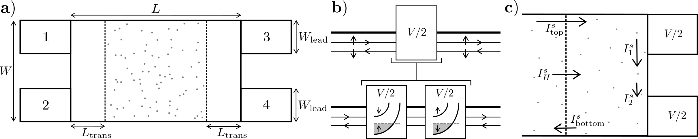
Figure 2: a) Schematic depiction of a four-terminal TI device of length $L$, width $W$, and lead width $W_{\text{lead}}$. The dotted region denotes disorder localized between two clean transition regions of length $L_{\text{trans}}$, where $L_{\text{trans}}=0$ indicates a fully disordered sample. We evaluate the spin conductances from the spin currents entering the terminals, see Eq. (26). b) In order to measure the spin current entering each terminal, we consider the terminals to be composed of two closely spaced ferromagnetic leads with magnetization axes parallel and anti-parallel to the quantized axis of the TI, see Eq. (24). c) Depiction of spin currents in the spin Hall setup, Fig. 1a, with spin-non-conserving disorder between leads 3 and 4. The spin Hall current $I^{s}_{H}$ passing through a cross section of the TI sample is conserved and equal to the sum of the currents along the top and bottom edges, $I^{s}_{H}=I^{s}_{\text{top}}+I^{s}_{\text{bottom}}$. However, spin-non-conserving disorder and a non-equilibrium distribution lead to a spin torque on the edge connecting terminals 3 and 4, see also Fig. 1b. Due to the spin torque, an additional current $\delta I^{s}_{H}=I^{s}_{1}-I^{s}_{2}$ is generated and flows to leads 3 and 4, resulting in a total spin current $I^{s}_{H}+\delta I^{s}_{H}$ entering the terminals and a non-quantized $G_{H}^{s}$.

We now move from the two-terminal case to a multiterminal system. While a two-terminal TI system requires the use of a proximitizing ferromagnetic heterostructure to drive a net spin current Götte et al. (2016), a spin Hall current can be driven purely electrically in a multiterminal setup. In this section we therefore give the relevant expressions for the currents and conductances necessary to study multiterminal charge and spin transport.

Consider a general $n$-terminal system with metallic leads attached. The full scattering matrix $\mathbb{S}$ of such a system relates the coefficients of the incoming modes $\Psi_{in}$ to the outgoing modes $\Psi_{out}$ by $\Psi_{out}=\mathbb{S}\Psi_{in}$. In particular, the $ij$-th block $\mathbb{S}_{ij}$ is the scattering matrix for modes scattering from terminal $j$ to $i$. Furthermore, in the case that the leads share a spin-rotational symmetry along a given axis, we may choose a new eigenbasis which conserves this symmetry. In this basis, the scattering matrix takes the form $\mathbb{S}_{i\sigma,j\sigma^{\prime}}$, where the $\sigma$ indices denote the spins of the incoming and outgoing modes.

The Landauer-Büttiker formula provides the charge current passing through a lead in the low temperature limit in terms of the voltages applied to the leads and the transmission coefficients $T_{ij}$ (from terminal $i$ to $j$):

$$I^{c}_{i}=\frac{e^{2}}{2\pi\hbar}\sum_{j\neq i}\left(T_{ji}V_{j}-T_{ij}V_{i}\right)\,.$$ (21)

In the case of spin-rotational symmetric leads, Eq. (21) may easily be generalized to give the spin-resolved current in a lead by considering each lead spin channel as a separate terminal:

$$I^{r}_{i\sigma}=\frac{e}{2\pi\hbar}\sum_{j\sigma^{\prime}\neq i\sigma}\left(T_{j\sigma^{\prime},i\sigma}V_{j}-T_{i\sigma,j\sigma^{\prime}}V_{i}\right)\,,$$ (22)

where the spin-resolved current $I^{r}_{i\sigma}$ is the outgoing current in lead $i$ due to electrons of spin $\sigma$. The charge and spin currents in each lead can then be related to these spin-resolved currents by

$$I^{c}_{i} =e\left(I^{r}_{i\uparrow}+I^{r}_{i\downarrow}\right)\,,$$ (23)

$$I^{s}_{i} =\frac{\hbar}{2}\left(I^{r}_{i\uparrow}-I^{r}_{i\downarrow}\right)\,.$$ (24)

The above equations also suggest that spin current can be measured by using two ferromagnetic terminals fully polarized along the $z$ and $-z$ axes. The net current into each terminal will be effectively spin resolved and their difference gives the net spin current. In Fig. 2b, we envision using this technique to measure the spin current into each terminal .

2-Terminal	$G^{c}_{2T}=G^{c}_{31}+G^{c}_{32}+G^{c}_{41}+G^{c}_{42}$
Incident	$G^{s}_{I}=-\frac{1}{2}\left(G^{s}_{11}-G^{s}_{12}+G^{s}_{21}-G^{s}_{22}\right)$
Transmitted	$G^{s}_{T}=\frac{1}{2}\left(G^{s}_{31}-G^{s}_{32}+G^{s}_{41}-G^{s}_{42}\right)$
Hall	$G^{s}_{H}=\frac{1}{2}\left(G^{s}_{31}-G^{s}_{32}+G^{s}_{33}-G^{s}_{34}\right.$
	$\left.+G^{s}_{41}-G^{s}_{42}+G^{s}_{43}-G^{s}_{44}\right)$
Diagonal Hall Kane and Mele (2005a)	$G^{s}_{D}=\frac{1}{2}\left(G^{s}_{31}-G^{s}_{34}\right)$

Table 1: Conductance definitions for various voltage setups in a four-terminal device. The terminal indexing matches Fig. 2; see Eqs. (25)–(26) for the matrix elements. The additional negative sign for the incident conductance ensures that positive current is defined to move to the right. Fig. 1 depicts the biasing setups (except for $G_{D}^{s}$).

In the scattering formalism, the conductance $\mathbf{G}$ of an $n$-terminal system is the $n\times n$ matrix relating the currents in the leads to the applied voltages. Assuming the leads share the same spin-rotational symmetry as the TI in the pristine limit, we define the $2n\times n$ spin-resolved conductance matrix $\mathbf{G}^{r}$ by the spin-resolved current response $I^{r}_{i\sigma}$ to a small voltage $V_{j}$ (setting all other voltages to zero): $G^{r}_{i\sigma,j}=I^{r}_{i\sigma}/V_{j}$. From this we then define the $n\times n$ charge and spin conductance matrices $\mathbf{G}^{c/s}$ by

$$G^{c}_{i,j} =e\left(G^{r}_{i\uparrow,j}+G^{r}_{i\downarrow,j}\right)=I^{c}_{i}/V_{j}\,,$$ (25)

$$G^{s}_{i,j} =\frac{\hbar}{2}\left(G^{r}_{i\uparrow,j}-G^{r}_{i\downarrow,j}\right)=I^{s}_{i}/V_{j}\,.$$ (26)

By inverting the conductance matrices, one could also quantify the inverse Hall effect and the inverse spin Hall effect, where a voltage is generated by a charge or spin current, respectively.

While the conductance matrices in Eqs. (25)–(26) provide the current response resulting from any voltage configuration, it is more illuminating to define conductance values for specific voltage setups such as those depicted in Fig. 1. In Table 1 we define several such conductance values for the four-terminal device depicted in Fig. 2a: the standard two-terminal charge conductance $G^{c}_{2T}$ due a horizontal potential bias, the incident and transmitted spin conductances $G^{s}_{I/T}$ due to a vertical bias on a single side, the spin Hall conductance $G^{s}_{H}$ due to a vertical bias on both sides, and the diagonal spin Hall conductance $G^{s}_{D}$ due to a diagonal bias (this was considered in Ref. Kane and Mele (2005a)). We note that in the case of $G^{s}_{D}$ there is a potential drop on every edge. This leads to $G^{s}_{D}$ being less robustly quantized than $G_{H}^{s}$, see Sec. III.3.

It is important to recognize that the spin conductances defined in Table 1 are defined with regards to the spin currents passing through the leads. In a multiterminal system with spin-non-conserving disorder this is not the same as spin currents passing through a cross section of the TI sample. In Fig. 2c we demonstrate this difference in the case of the spin Hall current and conductance. The net spin current into leads 3 and 4 on the right has two components: the spin Hall current from the left leads, $I^{s}_{H}$, and the extra spin current between leads 3 and 4, $\delta I^{s}_{H}$, generated by the spin torque from spin-non-conserving disorder, see Eq. (6). In terms of these, the spin Hall conductance is $G^{s}_{H}=\left(I^{s}_{H}+\delta I^{s}_{H}\right)/V$. In general, $G^{s}_{H}$ is not equal to the conductance corresponding to just the spin Hall current passing through the sample, $G^{s}_{H^{\prime}}=I^{s}_{H}/V$, especially when the connection between leads 3 and 4 is disordered (see Sec. III.3). Importantly, only $G^{s}_{H^{\prime}}$ is quantized as predicted in Sec. I when the entire sample is disordered; $G^{s}_{H}$ is only quantized when the connection between leads 3 and 4 has no spin-symmetry breaking disorder . This picture is confirmed by our numerical study where we compare clean and disordered connection between leads 3 and 4, see Fig. 7.

Using the definitions provided by Table 1, we can derive several relations between the four-terminal conductances. In particular, we consider two special cases which will be relevant to the results in Secs. III.1 and III.3. When the disorder does not break the spin-rotational symmetry of the TI, transmission between opposite spins is impossible: $T_{i\sigma,j\sigma^{\prime}}\propto\delta_{\sigma\sigma^{\prime}}$. This restriction results in the following relations between the conductances,

$$G^{s}_{H} =\frac{\hbar}{2e}G^{c}_{2T}\,,$$ (27)

$$G^{s}_{I} =G^{s}_{T}=\frac{1}{2}G^{s}_{H}\,.$$ (28)

The relations in Eqs. (27)–(28) are valid so long as every conducting state is spin-polarized and the spin-rotational symmetry remains unbroken. Meanwhile, if there is no inter-edge scattering then only spin-preserving transmission and spin-flipping reflections are allowed: $T_{i\sigma,j\sigma^{\prime}}\propto\absolutevalue{\delta_{ij}-\delta_{\sigma\sigma^{\prime}}}$. The resulting conductance relations are,

$$G^{s}_{T} =\frac{\hbar}{4e}G^{c}_{2T}\,,$$ (29)

$$G^{s}_{H} =G^{s}_{I}+G^{s}_{T}\,.$$ (30)

Unlike Eqs. (27)–(28), the relations in Eqs. (29)–(30) rely on the localization of the edge states and are not true in the presence of conducting bulk states.

III Numerical studies of disordered multiterminal systems

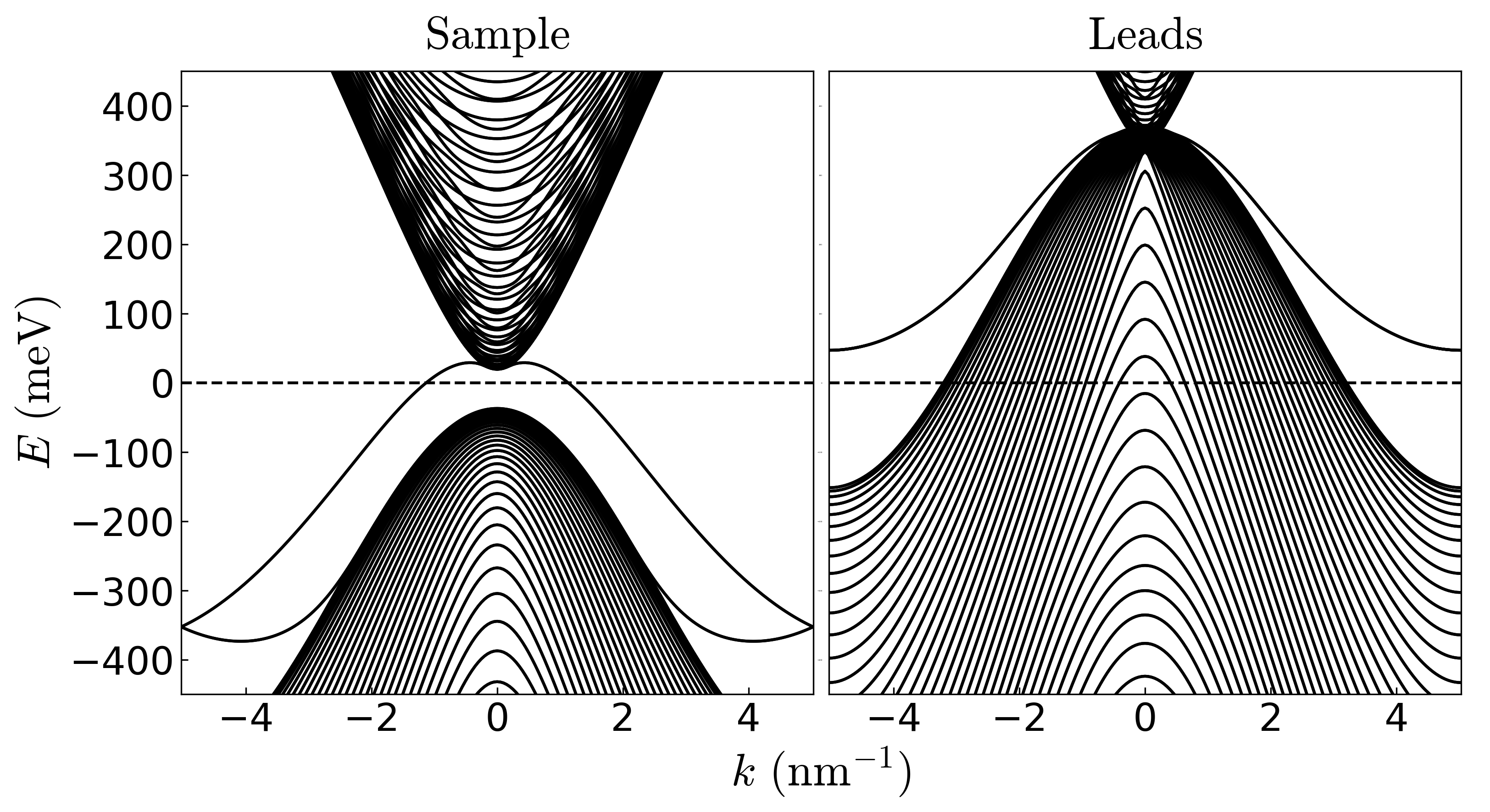
Figure 3: Straight-edge terminated WTe₂ band structure in a pristine sample (left) and leads (right), corresponding to the TI and metallic phases, respectively. The dashed line shows the chemical potential; the lead bands are shifted by $400$ meV relative to the sample.

To numerically study the transport properties of WTe₂, we utilized the Kwant package Groth et al. (2014) for Python to implement the tight-binding model introduced in Ref. Lau et al. (2019). Four-terminal systems were created to study the conductances in Table 1. Each system is comprised of a sample in the topological phase with four leads of width $W_{\text{lead}}=12$ nm attached at the corners, as depicted in Fig. 2. We model the leads with the same WTe₂ tight-binding model as the sample, except with spin-orbit coupling set to zero. The Fermi level of the leads is placed within the valence band ($\mu=-400$ meV) to allow for an abundance of conducting bulk modes; the sample Fermi level, meanwhile, is placed near the center of the 56 meV wide bulk gap ($E=0$ in Fig. 3) to ensure only edge modes are relevant in the pristine, zero-temperature limit. All plots shown utilize a horizontal straight-edge termination  that has a Dirac point buried within the valence band (see Fig. 3); however, we find similar results for the zigzag termination which has a Dirac point in the bulk gap. We then use Kwant to construct the scattering matrix for the system, which is used with Eqs. (22)–(26) to determine the charge and spin conductances in the zero-temperature limit .

Unless otherwise stated, each plot represents the average of $N=300$ disordered samples, which we find to be enough to limit most fluctuations (see Appendix C). We also attach the standard error bars for each plot (i.e. $\pm\sigma_{G}/\sqrt{N}$). For each plot we measure the conductances in terms of the charge and spin conductance quanta, $G^{c}_{0}=e^{2}/h$ and $G^{s}_{0}=e/(4\pi)$, respectively.

In the pristine limit we find the standard Kane and Mele (2005a) quantized values for the two-terminal charge conductance ($G^{c}_{2T}=2e^{2}/h$) and spin Hall conductance ($G^{s}_{H}=e/(2\pi)$). We also find that $G^{s}_{I}=G^{s}_{T}=e/(4\pi)$ and $G^{s}_{D}=e/(4\pi)$ Kane and Mele (2005a) in the pristine limit. In the following subsections we discuss the effects of on-site scalar and magnetic disorder on these results, in addition to disorder in the spin-orbit coupling parameters. We also study inter-edge scattering using a QPC system and calculate the characteristic spin decay length in the presence of magnetic disorder.

III.1 $S_{z}$ conserving disorder

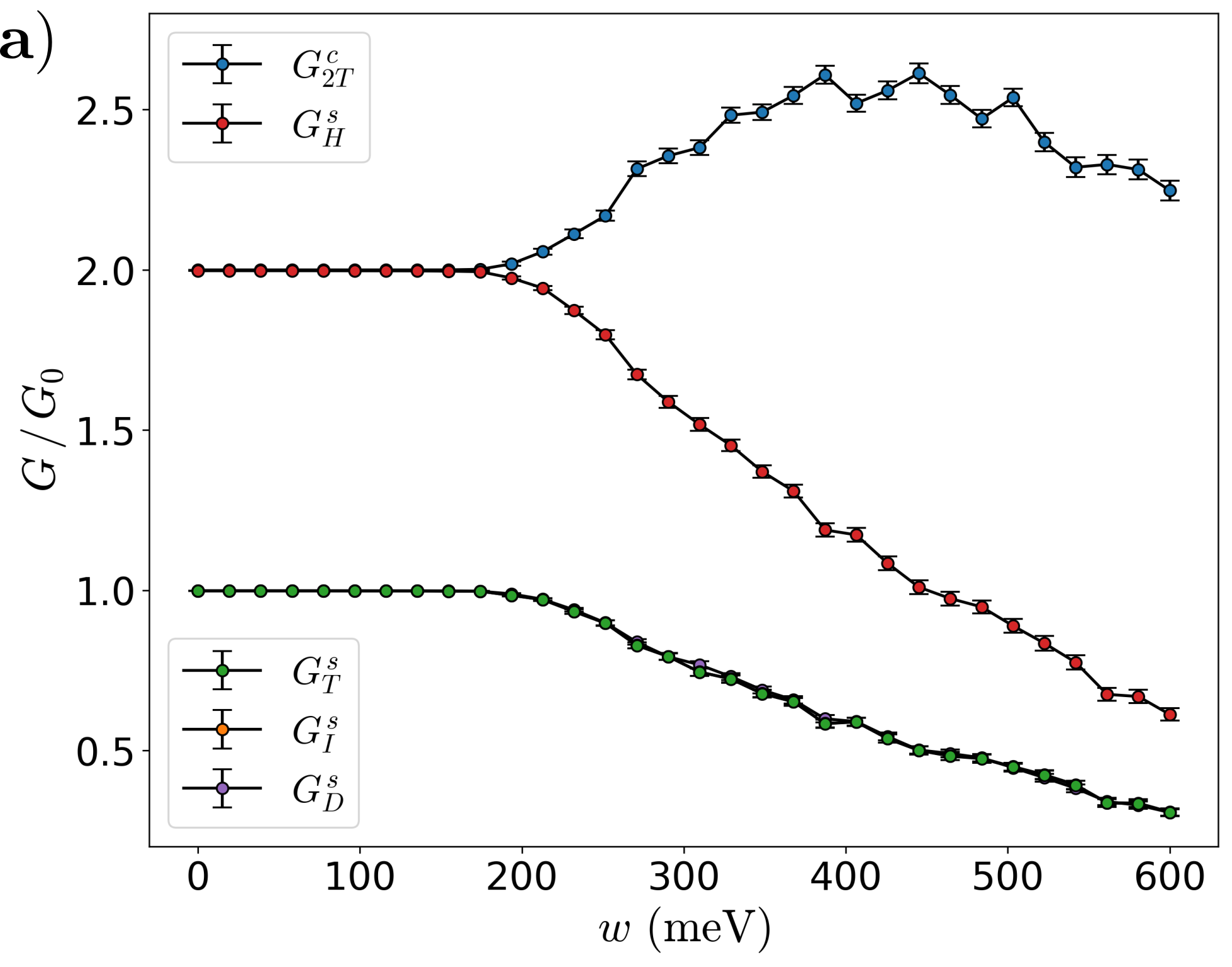
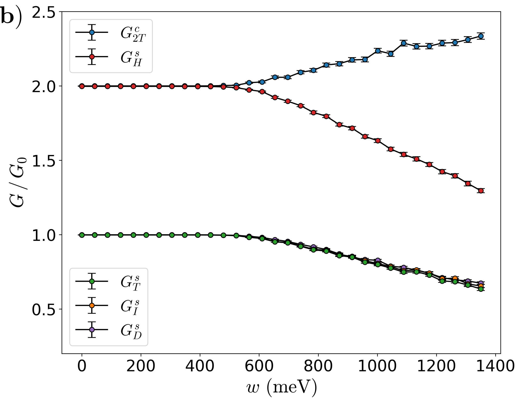
Figure 4: Conductances versus disorder strength $w$ for spin-conserving TR-symmetric perturbations. The system dimensions are $L=20$ nm, $W=30$ nm, $L_{\text{trans}}=0$, and $W_{\text{lead}}=12$ nm (see Fig. 2). Conductances are measured in units of the charge and spin conductance quanta. Note that the lowest 3 curves, $G^{s}_{T}$, $G^{s}_{I}$, and $G^{s}_{D}$, are overlapping over the full range of $w$ in both figures. a) On-site scalar disorder. b) Spin-conserving SOC disorder.

Due to the spin-momentum locking of the edge states in a 2D TI, it is expected that any perturbation which neither breaks the spin-symmetry nor couples the edges will not affect current propagation, as long as the perturbation strength is smaller than the gap to bulk excitations. Previous studies Lau et al. (2019); Li et al. (2009) have demonstrated this in the context of scalar disorder and charge conductance. Here, we demonstrate that weak spin-symmetric disorder does not affect the charge and spin conductance values of our four-terminal system. We study the effects of both on-site scalar disorder as well as disorder in the SOC strength.

In Fig. 4a we add a spatially-dependent on-site potential $u(\mathbf{x})$ drawn from a Gaussian of mean 0 and standard deviation $w$; we then plot the dependence of the conductances defined in Table 1 on $w$. For small enough values of $w$ ($<200$ meV), we find that the charge and spin conductances remain quantized at their expected values. This is due to the fact that scalar on-site disorder does not break the TR and spin-rotational symmetries of the TI, nor does it couple the two edges; the transmission amplitudes thus remain unaffected when the disorder is weak. At larger $w$, however, we see a decrease in the spin conductances and an increase in the charge conductance. The increasing charge conductance is attributable to the onset of bulk conduction within the disordered sample, whose size is smaller than the Anderson localization length. For weak disorder, the Fermi level of the sample remains within the bulk gap, ensuring that only the spin-momentum locked edge states effect the low-temperature conductances. Stronger disorder, meanwhile, can shift the bands sufficiently so that they cross the Fermi level, leading to bulk conduction.

The effect of disorder in the SOC strength is similar to spin-symmetric on-site disorder. In Fig. 4b we multiply the SOC strength by a spatially dependent factor $\lambda(\mathbf{x})$ drawn from a Gaussian of mean 1 and standard deviation $\delta\lambda$; we then plot the conductances versus $w=\lambda_{SOC}\delta\lambda$, where $\lambda_{SOC}=225$ meV is the sum of the SOC parameter magnitudes in the WTe₂ tight-binding model Lau et al. (2019) (see Appendix B for details on the WTe₂ tight-binding model). Importantly, this “isotropic” modification of the SOC strength does not change the spin quantization axis; this is unlike with anisotropic SOC disorder, see Sec. III.2 below. Just as with spin-symmetric on-site disorder, the conductances are robust against weak spin-symmetric SOC disorder; however, this regime appears to be smaller for SOC disorder, with the conductances deviating from their quantized values for $w>60$ meV.

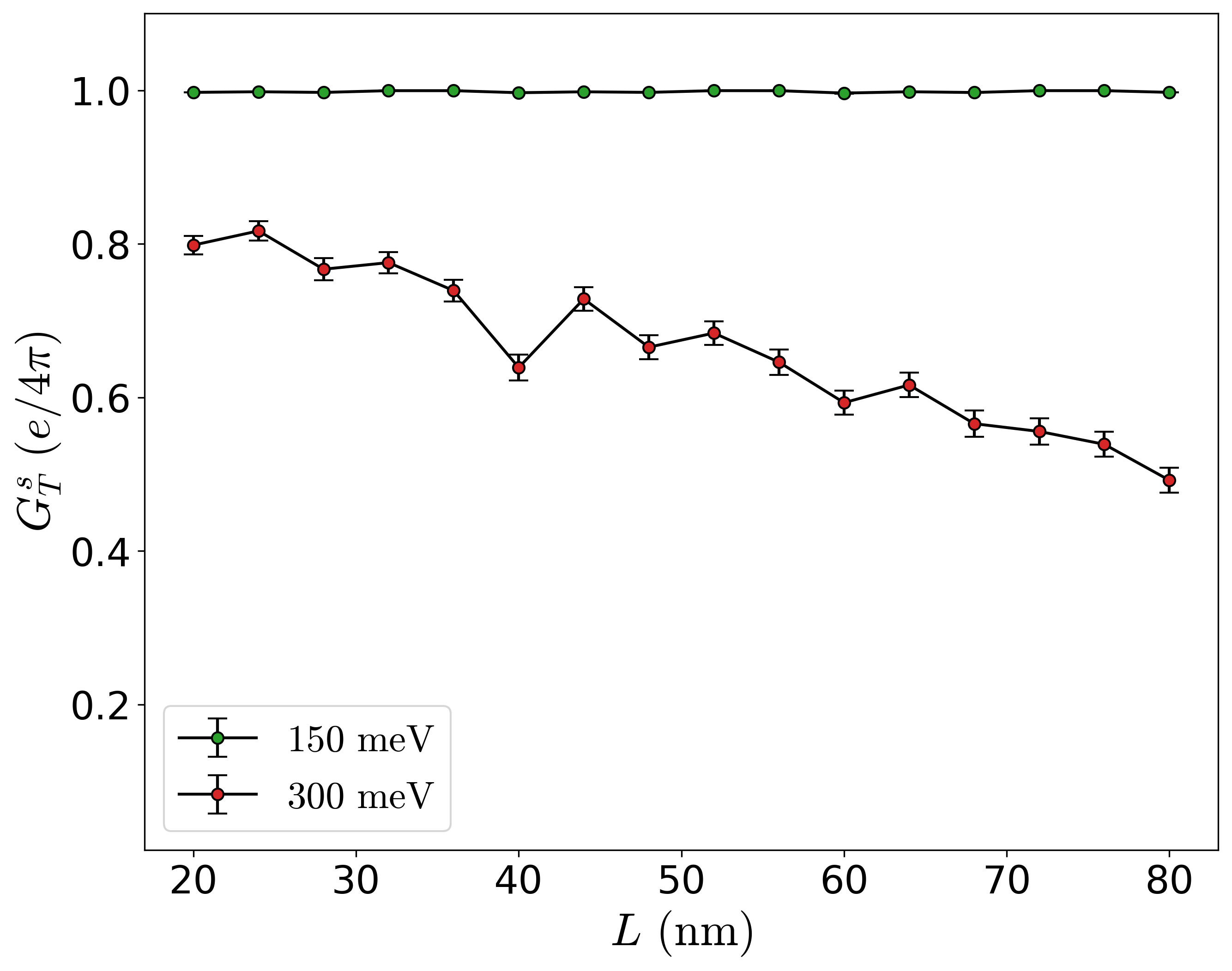
Figure 5: Transmitted spin conductance $G^{s}_{T}$ with on-site scalar disorder of width $w=150$ meV or $w=300$ meV versus sample length $L$. The other sample dimensions are $W=30$ nm, $L_{\text{trans}}=3$ nm, and $W_{\text{lead}}=12$ nm (see Fig. 2).

The conductances are remarkably robust against weak spin-symmetric disorder. In Fig. 5 we plot the transmitted spin conductance $G_{T}^{s}$ versus sample length for $w=150$ meV and $w=300$ meV on-site scalar disorder. In the weak disorder regime, the conductance remains quantized and does not appear to depend on the length up to $L=100$ nm (not shown). Weak length-dependence appears in the very strong disorder regime ($w>200$ meV for on-site scalar disorder). These findings are to be contrasted with a diffusive conductor where the conductance is inversely proportional to the length.

III.2 Time-reversal symmetric, $S_{z}$ non-conserving disorder

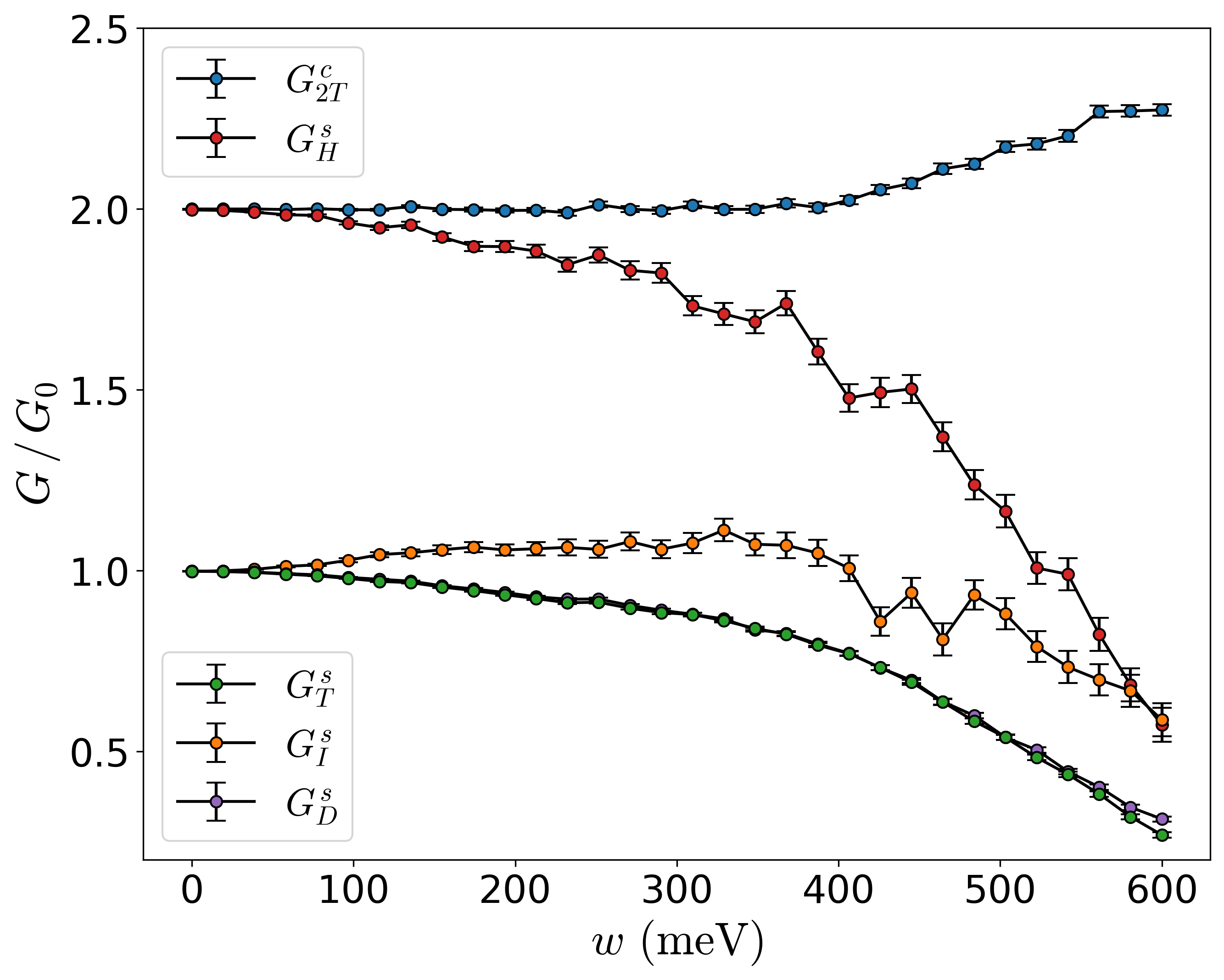
Figure 6: Conductances versus spin-non-conserving SOC disorder width $w$. The system dimensions are $L=20$ nm, $W=30$ nm, $L_{\text{trans}}=0$ nm, and $W_{\text{lead}}=12$ nm (see Fig. 2). Each data point represents the average of 500 samples. Conductances are measured in units of the charge and spin conductance quanta. Note that the $G^{s}_{T}$ and $G^{s}_{D}$ curves are overlapping over almost the full range of $w$.

In Sec. III.1 we saw that the charge and spin conductances remained quantized in the presence of weak on-site and SOC perturbations that do not break the spin-rotational symmetry of the TI. Here, we demonstrate that the conductances are not protected against SOC perturbations that break the spin-rotational symmetry, even when TR symmetry remains intact. In particular, we implement a TR-symmetric, $S_{z}$ non-conserving disorder term by adding a spatially-dependent $i\lambda^{\prime}_{0,x}(\mathbf{x})\sigma_{x}$ term to the $\lambda^{\prime}_{0}$ hopping amplitude, where $\lambda^{\prime}_{0,x}(\mathbf{x})$ is drawn from a Gaussian of mean 0 and standard deviation $w$ (see Appendix B). We demonstrate the effects of this term on the conductances in Fig. 6. As expected, SOC disorder that breaks $S_{z}$ conservation (Fig. 6) will lead to a stronger suppression of edge spin conductances as opposed to $S_{z}$ conserving SOC disorder (Fig. 4b).

For disorder terms weaker than $w<300$ meV, the conductances slowly deviate from their quantized values. This result suggests that TR symmetry alone is not enough to ensure quantization of the spin conductances when disorder is added to the SOC hopping amplitudes; rather, it is the combination of TR symmetry and spin-rotational symmetry that leads to this quantization. Of course, this distinction is not relevant when one only considers on-site disorder terms, as in that case spin-rotational symmetry is implied by TR symmetry. At larger $w$ we see a qualitatively different dependence of conductance on disorder strength, corresponding to the onset of bulk conduction in the disordered sample. While the conductances do not remain quantized in the presence of TR-symmetric, spin-non-conserving disorder, their deviations from their quantized values appears to be much weaker than for disorder that breaks TR symmetry, see Fig. 7b in Sec. III.3.

III.3 Magnetic disorder breaking time-reversal symmetry and $S_{z}$ conservation

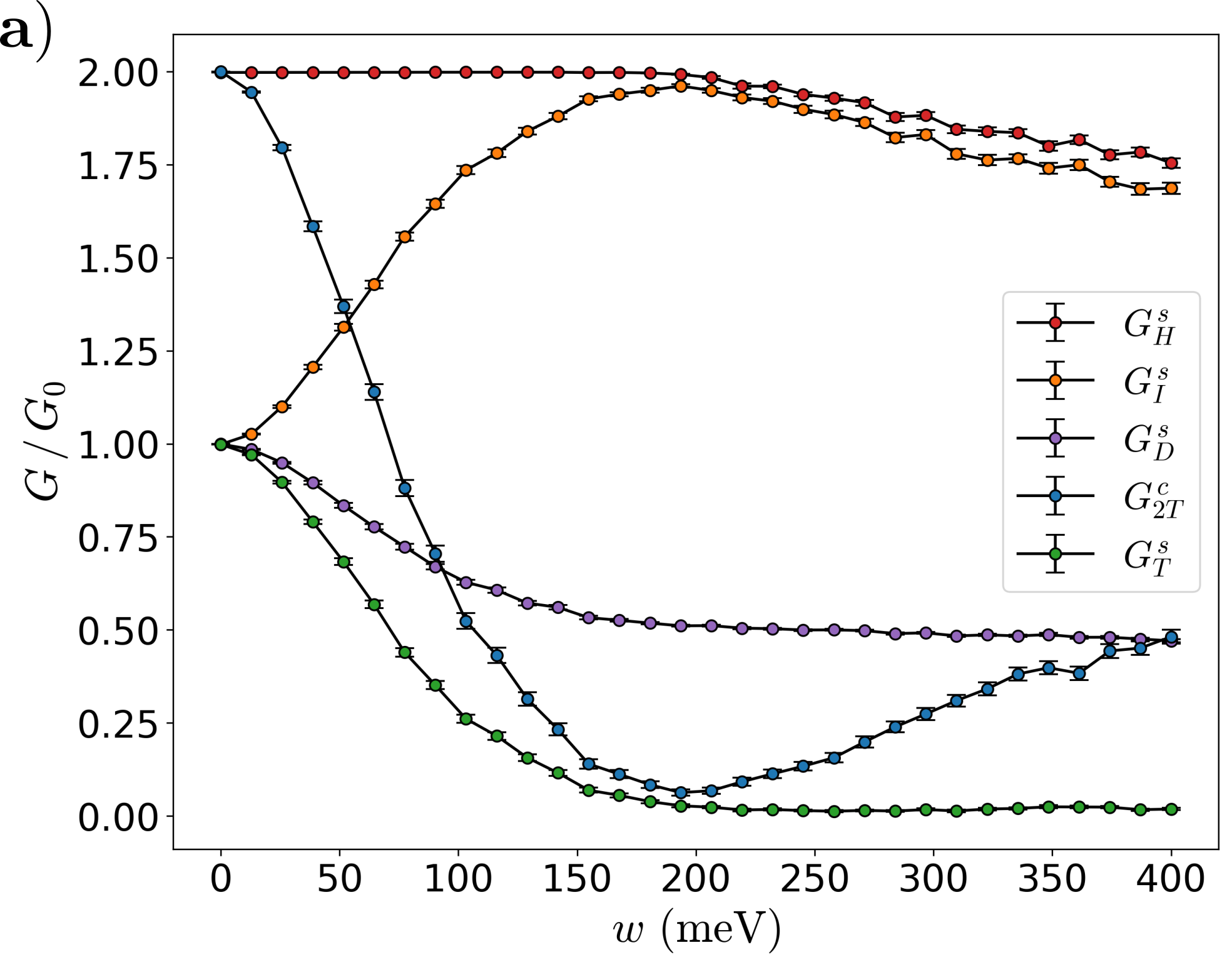
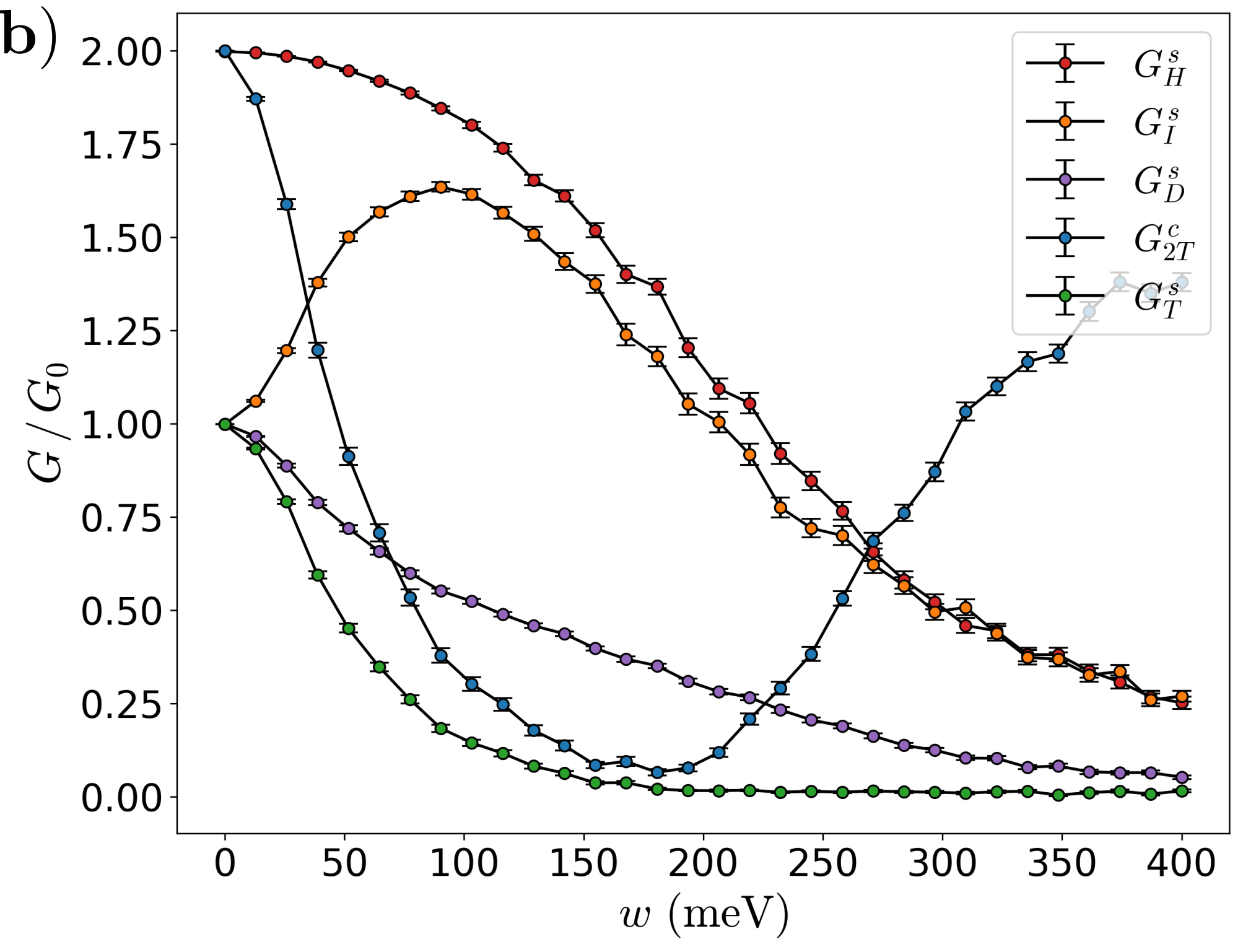
Figure 7: Conductances versus on-site magnetic disorder width $w$. For both plots $L=20$ nm, $W=30$ nm, and $W_{\text{lead}}=12$ nm (see Fig. 2). Conductances are measured in units of the charge and spin conductance quanta. a) A $L_{\text{trans}}=2.5$ nm wide clean transition region is added to the ends of the TI to ensure no disorder at the lead-TI interfaces. In this case the spin current entering the terminals is approximately conserved and $G^{s}_{H}$ stays quantized up to large $w\lesssim 200$ meV. b) No such transition region is added, $L_{\text{trans}}=0$. In this case there is a spin torque that prevents the quantization of $G^{s}_{H}$, see Fig. 2c.

Unlike spin-symmetric on-site disorder and SOC disorder, unaligned magnetic disorder breaks both the TR symmetry and the spin-rotational symmetry of the TI, leading to a large deviation of the conductance from the pristine-limit quantization even before the onset of bulk conduction. To demonstrate this, we add a $m(\mathbf{x})\sigma_{x}$ on-site disorder term, where $m(\mathbf{x})$ is once again drawn from a Gaussian of mean 0 and standard deviation $w$. We also show how the conductances defined in the leads depend drastically on whether or not there is disorder along the left and right edges.

In Fig. 7a we demonstrate the case of magnetic disorder localized such that there is no disorder between leads of the same side ($L_{\text{trans}}=2.5$ nm in Fig. 2). We see that the spin Hall conductance $G^{s}_{H}$ maintains its quantized value until the onset of bulk conduction at about $w=200$ meV, demonstrating the robustness predicted by Eq. (15). Meanwhile, the charge conductance $G^{c}_{2T}$ and transmitted spin conductance $G^{s}_{T}$ immediately begin to decrease with $w$ while the incident spin conductance $G^{s}_{I}$ increases. These deviations are in qualitative agreement with Eqs. (10)–(11) if we make the identification $\eta_{m}=w^{2}x_{0}r_{0}/(\hbar^{2}v^{2})$, where $x_{0}=L-2L_{\text{trans}}$ is the length of the disordered region and $r_{0}$ is the correlation length of the disorder. The conductances also obey the relations predicted by Eqs. (29)–(30). Similarly, the diagonal spin Hall conductance $G^{s}_{D}$ deviates from its quantized value at a much lower strength of disorder than $G^{s}_{H}$. We attribute this difference to the different biasing configurations: in measuring $G^{s}_{D}$, every edge has a voltage drop which allows for large spin torque contributions (see Sec. I). We also note that $G^{s}_{D}$ appears to decrease to half of its zero-disorder quantized value. This is due to the fact that in Table 1 for very strong disorder $G^{s}_{31}\to 0$ but $G^{s}_{34}=-1$ due to the clean connection between leads 3 and 4.

Meanwhile, in Fig. 7b, we demonstrate the case of a fully-disordered sample with magnetic disorder added along the edges connecting leads of the same side ($L_{\text{trans}}=0$ in Fig. 2). We see that the removal of the clean connection results in a different dependence on the disorder strength. The relations given by Eqs. (29)–(30), which only relied on the lack of bulk conduction and edge-to-edge coupling, still hold for $w<200$ meV. However, the spin Hall conductance $G^{s}_{H}$ is apparently no longer quantized, and the deviations of $G^{s}_{I}$ and $G^{s}_{T}$ no longer agree with what is predicted by Eqs. (10)–(11). As mentioned in Sec. II, this discrepancy is due to the fact that we define the conductances in the leads, not in the sample. We expect the spin Hall conductance corresponding to the current in the sample to remain quantized even when the sample is strongly disordered.

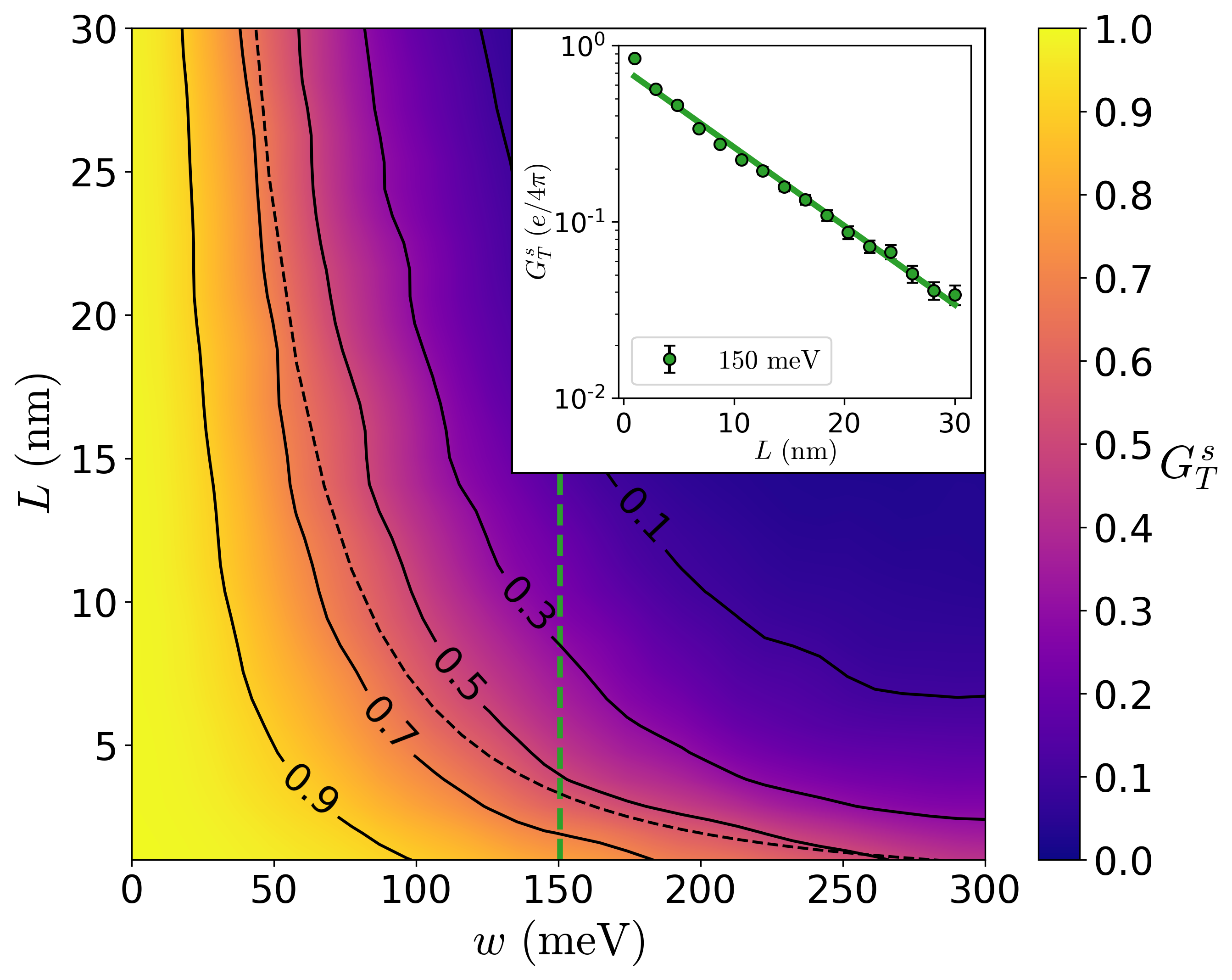
Figure 8: Transmitted spin conductance $G^{s}_{T}$ as a function of sample length $L$ and on-site magnetic disorder width $w$ for a 32 by 32 mesh grid. The other sample dimensions are $W=30$ nm, $L_{\text{trans}}=3$ nm, and $W_{\text{lead}}=12$ nm (see Fig. 2a). The average value of $G^{s}_{T}$ over 50 samples was used to color each grid point; the plot was then smoothed using a Gaussian. The solid lines are contours of constant $G^{s}_{T}$ and roughly follow a $L\propto w^{-2}$ dependence (black dashed line), as is predicted by the relation $\ln G^{s}_{T}\propto-Lw^{2}$. Inset: Logarithmic plot of $G^{s}_{T}$ averaged over 300 samples versus $L$ for a fixed $w=150$ meV slice (green dashed line in the main figure). The slope of the best fit line (solid green) is $-1/(9.7\,\text{nm})$.

In addition to studying how the disorder strength affects the conductances, we also study how the transmitted conductance $G^{s}_{T}$ varies with the sample length $L$. We plot the dependence of $G^{s}_{T}$ on the disorder strength and sample length, as well as a constant $w=150$ meV slice, in Fig. 8. We find that, for constant $w$, the transmitted spin conductance decays exponentially with the sample length, i.e. $G^{s}_{T}\propto e^{-L/l_{0}}$ where $l_{0}$ is a characteristic spin decay length. For $w=150$ meV, our fit gives $l_{0}\approx 9.7$ nm, see inset of Fig. 8. This roughly agrees with an estimate of $l_{0}=\hbar^{2}v^{2}/(w^{2}r_{0})\approx 3.2$ nm if we use the average distance between neighboring lattice sites $r_{0}\approx.2$ nm as a disorder correlation radius and $\hbar v\approx 120\,\mathrm{meV}\cdot\mathrm{nm}$ estimated from Fig. 3.

III.4 Quantum point contact system

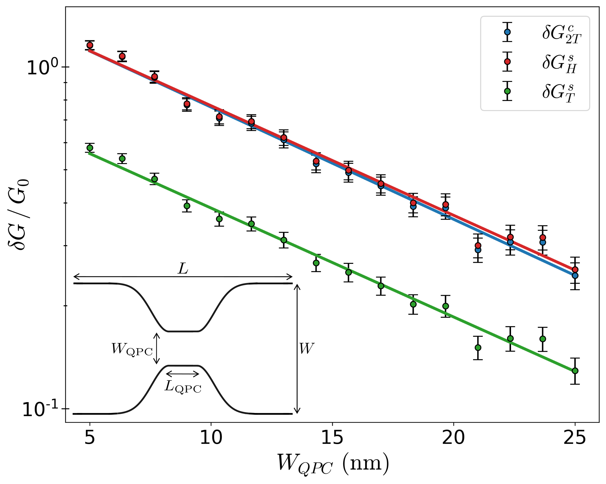
Figure 9: Conductance deviations $\delta G=G_{0}-G$ of a four-terminal QPC system made of a $L=30$ nm by $W=30$ nm rectangular sample cut such that the width smoothly transitions to a narrowed region of length $L_{\text{QPC}}=200$ nm and varying width $W_{\text{QPC}}$. A scalar disorder term with standard deviation $w=300$ meV is then added to extend the effective decay length and increase edge-to-edge coupling. Conductance deviations are measured in units of the charge and spin conductance quanta. The slopes of the corresponding best fit lines are $-1/(13.2\,\text{nm})$ for $G^{c}_{2T}$, $-1/(13.6\,\text{nm})$ for $G^{s}_{H}$, and $-1/(13.5\,\text{nm})$ for $G^{s}_{T}$. Inset: Diagram of the QPC device demonstrating the definitions of the various dimensions.

As mentioned in Sec. I, inter-edge tunneling through the bulk of the TI is another mechanism by which the conductances can deviate from their quantized values. For each conductance $G$ we define the deviation $\delta G$ from the quantized value $G(w=0)$ by $\delta G=G(w=0)-G$. In a QPC system of minimum width $W_{\text{QPC}}$, we expect $\delta G\propto e^{-W_{\text{QPC}}/W_{0}}$ for $W_{\text{QPC}}\gg W_{0}$, where $W_{0}$ is the effective decay length of the edge modes (not to be confused with the characteristic spin decay length $l_{0}$ studied in Sec. III.3). To test this relation, we create a four-terminal QPC system where a rectangular sample is smoothly transitioned into a narrowed region of width $W_{\text{QPC}}$ and length $L_{\text{QPC}}$ (see inset of Fig. 9). We then add a scalar disorder term to extend the effective decay length $W_{0}$.

In Fig. 9 we plot the resulting conductance deviations against $W_{\text{QPC}}$ on a logarithmic scale, along with their linear fits. Using the inverse slopes of the best fit lines, we find that the decay lengths of each conductance component is roughly 13 nm. The various spin conductance deviations, including the incident and diagonal conductance deviations which we hide for clarity, have similar decay lengths. Physically, the decay length serves as an indicator of the edge state width in the QPC geometry. We note that each conductance component decays at the same rate as is expected from Eqs. (27)–(28), valid for a system with spin conservation .

IV Conclusions

We studied the effects of disorder on spin transport in 2D TIs and established important estimates for the level of disorder strength that starts to hinder spin transport. One of our main findings is that the spin current operator on the 2D TI edge is given by the local density, Eq. (14). For this reason, the spin Hall current generated by a transverse voltage is remarkably robust to even spin-non-conserving perturbations, see Eq. (15), as long as the two edges of the 2D TI are not coupled. However, measuring the spin Hall current in a 4-terminal geometry is difficult due to additional spin currents that flow between the terminals at different potentials, see Fig. 2c. These spin currents are not in general conserved and hinder the measurement of a quantized spin Hall conductance. These findings are confirmed by our numerical simulations, e.g. Fig. 7. Overall, we find that spin conductance is most sensitive to spin-non-conserving disorder such as random spin-orbit coupling (Fig. 6) or magnetic impurities (Figs. 7–8). In the former time-reversal symmetric case, the spin Hall conductance is nevertheless nearly quantized even with relatively large disorder strength of the order of the bulk band gap.

In WTe₂, recent measurements of the spin quantization axis indicate that spin-orbit disorder is relatively weak. The canting of the edge state spin has been measured in experiments Tan et al. (2021); Zhao et al. (2021) in agreement with theoretical models Garcia et al. (2020); Arora et al. (2020); Ok et al. (2019); Lau et al. (2019); Nandy and Pesin (2021). These findings indicate that the spin quantization axis, although canted, does not vary strongly in position or momentum space. This gives hope that the spin of the edge carriers can be conserved over long distances.

We focused on low-temperatures at which scattering is dominated by elastic processes. At the same time, we found that time-reversal symmetric disorder has a weak effect on spin transport, see Secs. III.1–III.2. Therefore, at higher temperatures, inelastic scattering is expected to become the dominant scattering mechanism, leading to temperature-dependent corrections to the spin conductances. Finite-temperature and interaction effects on spin transport constitute an interesting future direction (see also Refs. Teo and Kane (2009); Hou et al. (2009); Ström and Johannesson (2009) for quantum point contacts). Other intriguing future directions would be to study the details of the tunnel-coupling between a TI edge and a ferromagnetic contact Yokoyama and Tserkovnyak (2014); Scharf et al. (2016); Sayed et al. (2016); Davidson et al. (2020) or the effects of electric fields in relatively clean systems and investigate the potential to control spin polarization electrically Farzaneh and Rakheja (2021).

Appendix A Derivation of transmission and reflection coefficients

Here we derive the transmission $t$ and reflection $r$ coefficients given by Eqs. (7)–(8). We first find the eigenstates of Eq. (5) by rearranging the Schrödinger equation $\mathcal{H}(x)\psi=E\psi$ into a more convenient form,

$$\partial_{x}\psi=\frac{1}{\hbar v}\left[m(x)\sigma_{y}+i(E+\mu)\sigma_{z}\right]\psi\,,$$ (31)

which can then be solved through the use of a matrix exponential:

$$\psi(x_{0})=\exp{\eta_{m}\sigma_{y}+i\xi\sigma_{z}}\psi(0)\,,$$ (32)

where $\eta_{m}=\int_{0}^{x_{0}}m(x)dx/(\hbar v)$ and $\xi=(E+\mu)x_{0}/(\hbar v)$. Thus, by taking $0/x_{0}$ to be at the left/right edges of the disordered region and expanding the matrix exponential in Eq. (32), we can calculate how the disorder scatters an incoming mode. Defining $\chi=\sqrt{\xi^{2}-\eta_{m}^{2}}$, the matrix exponential in Eq. (32) is equal to the scattering operator

$$\hat{S}=\cos{\chi}+\frac{\eta_{m}\sigma_{y}+i\xi\sigma_{z}}{\chi}\sin{\chi}\,.$$ (33)

To calculate the transmission/reflection coefficient of an incoming right-mover, we apply $\hat{S}$ to the state $\psi(0)=\ket{\uparrow}+r\ket{\downarrow}$, where $r$ is the reflection amplitude yet to be determined:

$$\begin{split}\psi(x_{0})&=\hat{S}\psi(0)\\ &=\left[\cos{\chi}+i\frac{\xi}{\chi}\sin{\chi}-ir\frac{\eta_{m}}{\chi}\sin{\chi}\right]\ket{\uparrow}\\ &+\left[r\cos{\chi}-ir\frac{\xi}{\chi}\sin{\chi}+i\frac{\eta_{m}}{\chi}\sin{\chi}\right]\ket{\downarrow}\,.\end{split}$$ (34)

Since the spin-down state on the right side of the barrier is an incoming left-mover, we know its coefficient must be zero. Hence, solving for $r$ and plugging the result into the spin-up coefficient for $t$ gives

$$t =\frac{\chi^{2}\cos{\chi}+i\xi\chi\sin{\chi}}{\xi^{2}-\eta_{m}^{2}\cos^{2}{\chi}}\,,$$ (35)

$$r =\frac{\eta_{m}\xi\sin^{2}{\chi}-i\eta_{m}\chi\sin{\chi}\cos{\chi}}{\xi^{2}-\eta^{2}_{m}\cos^{2}\chi}\,.$$ (36)

Finally, we note that a similar analysis using an incoming left-mover gives the same coefficients, resulting in a unitary scattering matrix as given by Eq. (9) in the low-energy limit. Furthermore, the square magnitudes $\absolutevalue{t}^{2}$ and $\absolutevalue{r}^{2}$ are (restoring $\chi=\sqrt{\xi^{2}-\eta_{m}^{2}}$)

$$\absolutevalue{t}^{2} =\frac{\xi^{2}-\eta_{m}^{2}}{\xi^{2}-\eta_{m}^{2}\cos^{2}{\sqrt{\xi^{2}-\eta_{m}^{2}}}}\,,$$ (37)

$$\absolutevalue{r}^{2} =\frac{\eta_{m}^{2}\sin^{2}{\sqrt{\xi^{2}-\eta_{m}^{2}}}}{\xi^{2}-\eta_{m}^{2}\cos^{2}{\sqrt{\xi^{2}-\eta_{m}^{2}}}}\,.$$ (38)

Taking the scattering state near the Dirac point, ${\xi\ll\eta_{m}}$, these expressions are used in Eqs. (10)–(11) to calculate the spin current on the left and right of the disordered edge segment.

Appendix B Tight-binding model

(Note: in this Appendix we denote $\mathbf{z}$ the axis perpendicular to the monolayer, while the spin quantization axis, denoted here $\mathbf{z}^{\prime}$, is tilted with respect to the normal (see the end of this section). In the main text we drop the prime from $\mathbf{z}^{\prime}$ for brevity.) Here we reproduce the tight-binding model introduced in Ref. Lau et al. (2019) and detail the disorder terms used in Sec. III. WTe₂ in the $1T^{\prime}$ configuration consists of a square lattice with six atoms per unit cell. The effective tight-binding model introduced by Ref. Lau et al. (2019) reduces this to a four-site square lattice, with two $d_{x^{2}-y^{2}}$ (W) orbitals and two $p_{x}$ (Te) orbitals per cell.

Adopting the notation of Ref. Lau et al. (2019), we define the Pauli matrices $s_{i}$, $\tau_{i}$, and $\sigma_{i}$ to act on the spin, sublattice, and orbital degrees of freedom, respectively, and define the $\Gamma_{i}$ matrices by

$$\Gamma_{0} =\tau_{0}\sigma_{0}\,,$$ (39)

$$\Gamma^{\pm}_{1} =\frac{1}{2}\tau_{0}(\sigma_{0}\pm\sigma_{3})\,,$$ (40)

$$\Gamma^{\pm}_{2} =\frac{1}{4}(\tau_{1}+i\tau_{2})(\sigma_{0}\pm\sigma_{3})\,,$$ (41)

$$\Gamma_{3} =\frac{i}{2}(\tau_{1}+i\tau_{2})\sigma_{2}\,,$$ (42)

$$\Gamma^{\pm}_{4} =\frac{1}{4}(\tau_{0}\pm\tau_{3})(\sigma_{1}+i\sigma_{2})\,,$$ (43)

$$\Gamma^{\pm}_{5} =\frac{1}{2}\tau_{3}(\sigma_{0}\pm\sigma_{3})\,,$$ (44)

$$\Gamma_{6} =\frac{1}{2}(\tau_{1}+i\tau_{2})\sigma_{1}\,.$$ (45)

To be explicit, a term of the form $s_{i}\tau_{j}\sigma_{k}$ acts on the operator

$$\begin{split}c_{\vec{r}}=[&c_{\vec{r}\,\uparrow Ad},\,c_{\vec{r}\,\uparrow Ap},\,c_{\vec{r}\,\uparrow Bd},\,c_{\vec{r}\,\uparrow Bp},\\ &c_{\vec{r}\,\downarrow Ad},\,c_{\vec{r}\,\downarrow Ap},\,c_{\vec{r}\,\downarrow Bd},\,c_{\vec{r}\,\downarrow Bp}]\,,\end{split}$$ (46)

where $c_{\vec{r}slo}$ annihilates a spin $s\in\{\uparrow,\downarrow\}$ electron on sublattice $l\in\{A,B\}$ and orbital $o\in\{d,p\}$.

With these definitions, the tight-binding Hamiltonian can be written as $H=\sum_{\vec{r}}\left[H_{0}(\vec{r})+\lambda(\vec{r})H_{\mathrm{SOC}}(\vec{r})+\delta H(\vec{r})\right]$, where Lau et al. (2019)

$$\begin{split}H_{0}(\vec{r})&=\frac{\mu_{d}}{2}c^{\dagger}_{\vec{r}}\,\Gamma^{+}_{1}c_{\vec{r}}+\frac{\mu_{p}}{2}c^{\dagger}_{\vec{r}}\,\Gamma^{-}_{1}c_{\vec{r}}\\ &+\frac{t_{dx}}{2}c^{\dagger}_{\vec{r}}\,\Gamma^{+}_{1}(c_{\vec{r}+\vec{a}}+c_{\vec{r}-\vec{a}})\\ &+\frac{t_{px}}{2}c^{\dagger}_{\vec{r}}\,\Gamma^{-}_{1}(c_{\vec{r}+\vec{a}}+c_{\vec{r}-\vec{a}})\\ &+\frac{t_{py}}{2}c^{\dagger}_{\vec{r}}\,\Gamma^{-}_{1}(c_{\vec{r}+\vec{b}}+c_{\vec{r}-\vec{b}})\\ &+t_{dAB}\,c^{\dagger}_{\vec{r}}\,\Gamma^{+}_{2}(c_{\vec{r}-\vec{b}+\vec{\Delta}_{1}}+c_{\vec{r}+\vec{a}-\vec{b}+\vec{\Delta}_{1}})\\ &+t_{pAB}\,c^{\dagger}_{\vec{r}}\,\Gamma^{-}_{2}(c_{\vec{r}+\vec{\Delta}_{2}}+c_{\vec{r}+\vec{a}+\vec{\Delta}_{2}})\\ &+t_{0AB}\,c^{\dagger}_{\vec{r}}\,\Gamma_{3}(c_{\vec{r}+\vec{\Delta}_{3}}-c_{\vec{r}+\vec{a}+\vec{\Delta}_{3}})\\ &-t_{0x}\,c^{\dagger}_{\vec{r}}\,\Gamma^{+}_{4}(c_{\vec{r}+\vec{a}+\vec{\Delta}_{4}}-c_{\vec{r}-\vec{a}+\vec{\Delta}_{4}})\\ &-t_{0x}\,c^{\dagger}_{\vec{r}}\,\Gamma^{-}_{4}(c_{\vec{r}+\vec{a}-\vec{\Delta}_{4}}-c_{\vec{r}-\vec{a}-\vec{\Delta}_{4}})\\ &+t_{0ABx}\,c^{\dagger}_{\vec{r}}\,\Gamma_{3}(c_{\vec{r}-\vec{a}+\vec{\Delta}_{3}}-c_{\vec{r}+2\vec{a}+\vec{\Delta}_{3}})\\ &+\mathrm{H.c.}\,,\end{split}$$ (47)

and

$$\begin{split}H_{\mathrm{SOC}}(\vec{r})&=-\frac{i}{2}c^{\dagger}_{\vec{r}}\,(\lambda^{z}_{dx}s_{z}+\lambda^{y}_{dx}s_{y})\Gamma^{+}_{5}(c_{\vec{r}+\vec{a}}-c_{\vec{r}-\vec{a}})\\ &-\frac{i}{2}c^{\dagger}_{\vec{r}}\,(\lambda^{z}_{px}s_{z}+\lambda^{y}_{px}s_{y})\Gamma^{-}_{5}(c_{\vec{r}+\vec{a}}-c_{\vec{r}-\vec{a}})\\ &-i\lambda^{y}_{0AB}c^{\dagger}_{\vec{r}}\,s_{y}\Gamma_{6}(c_{\vec{r}+\vec{\Delta}_{3}}+c_{\vec{r}+\vec{a}+\vec{\Delta}_{3}})\\ &-ic^{\dagger}_{\vec{r}}\,(\lambda^{z}_{0}s_{z}+\lambda^{y}_{0}s_{y})\Gamma^{+}_{4}c_{\vec{r}+\vec{\Delta}_{4}}\\ &+ic^{\dagger}_{\vec{r}}\,(\lambda^{z}_{0}s_{z}+\lambda^{y}_{0}s_{y})\Gamma^{-}_{4}c_{\vec{r}-\vec{\Delta}_{4}}\\ &-ic^{\dagger}_{\vec{r}}(\lambda^{\prime z}_{0}s_{z}+\lambda^{\prime y}_{0}s_{y})\Gamma^{+}_{4}c_{\vec{r}-\vec{b}+\vec{\Delta}_{4}}\\ &+ic^{\dagger}_{\vec{r}}(\lambda^{\prime z}_{0}s_{z}+\lambda^{\prime y}_{0}s_{y})\Gamma^{-}_{4}c_{\vec{r}+\vec{b}-\vec{\Delta}_{4}}\\ &+\mathrm{H.c.}\,,\end{split}$$ (48)

are the spin-rotation symmetric and spin-orbit coupling terms, respectively, $\lambda(\vec{r})$ is a potentially site-dependent scale factor modifying the SOC strength ($\lambda(\vec{r})=1$ for physical WTe₂ and $=0$ for no SOC), and $\delta H(\vec{r})$ describes any additional disorder terms. The parameter values used in Eqs. (47)–(47) can be found in Table 2.

$H_{0}$ (eV)		$H_{\mathrm{SOC}}$ (meV)
$\mu_{d}$	0.24	$\lambda^{z}_{dx}$	-8
$\mu_{p}$	-2.25	$\lambda^{y}_{dx}$	-31
$t_{dx}$	-0.41	$\lambda^{z}_{px}$	-10
$t_{px}$	1.13	$\lambda^{y}_{px}$	-40
$t_{py}$	0.13	$\lambda^{y}_{0AB}$	11
$t_{dAB}$	0.51	$\lambda^{z}_{0}$	12
$t_{pAB}$	0.4	$\lambda^{y}_{0}$	51
$t_{0AB}$	0.39	$\lambda^{\prime z}_{0}$	12
$t_{0x}$	0.14	$\lambda^{\prime y}_{0}$	50
$t_{0ABx}$	0.29

Table 2: Parameter values used in the tight-binding model of 1T’-WTe₂ Lau et al. (2019) (see Eqs. (47)–(48)).

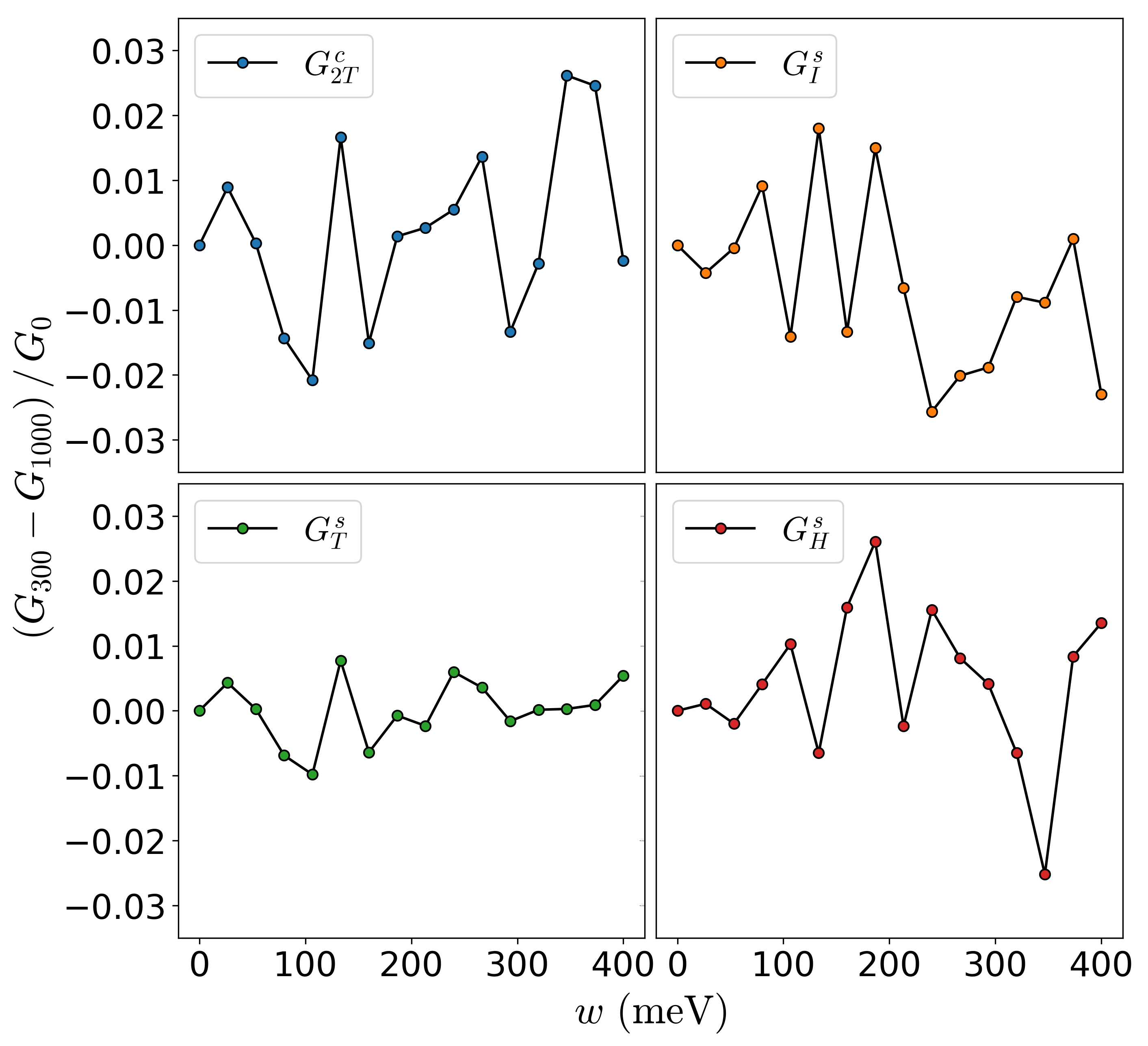
Figure 10: Normalized differences between 300 sample and 1000 sample averages. The disorder term is a localized magnetic perturbation as discussed in Sec. III.3 and shown in Fig. 7b.

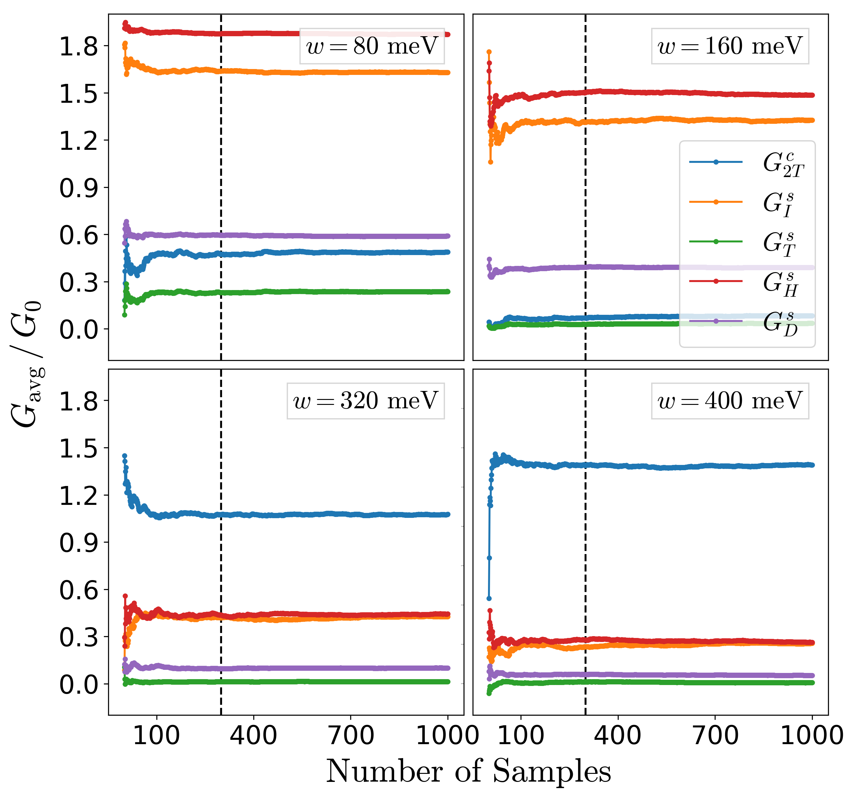
Figure 11: Disorder-averaged conductance components versus the number of samples used at fixed $w$. The disorder term is a localized magnetic perturbation as discussed in Sec. III.3 and shown in Fig. 7b.

In Sec. III we study the effects of several on-site and hopping disorder terms. In Sec. III.1 we study on-site scalar disorder terms of the form $\delta H(\vec{r})=u(\vec{r})c^{\dagger}_{\vec{r}}\,s_{0}\Gamma_{0}c_{\vec{r}}$, where $u(\vec{r})$ is drawn from a Gaussian of mean 0 and standard deviation $w$. We also study spin-conserving disorder in the SOC strength by having $\lambda(\vec{r})$ be drawn from a Gaussian of mean 1 and standard deviation $\delta\lambda$. In Sec. III.2 we break spin-rotational symmetry (while preserving TR symmetry) by adding a disorder term $\delta H(\vec{r})=i\lambda^{\prime x}_{0}(\vec{r})c^{\dagger}_{\vec{r}}s_{x}(\Gamma^{+}_{4}c_{\vec{r}-\vec{b}+\vec{\Delta}_{4}}-\Gamma^{-}_{4}c_{\vec{r}+\vec{b}-\vec{\Delta}_{4}})+\mathrm{H.c.}$, with $\lambda^{\prime x}_{0}(\vec{r})$ drawn from a Gaussian of mean 0 and standard deviation $w$. Finally, in Sec. III.3 we break both TR and spin-rotational symmetry by including an on-site perturbation $\delta H(\vec{r})=m(\vec{r})c^{\dagger}_{\vec{r}}\,s_{x}\Gamma_{0}c_{\vec{r}}$, with $m(\vec{r})$ once again drawn from a Gaussian of mean 0 and standard deviation $w$.

Finally, we comment on the edge state spin quantization axis of a pristine WTe₂ obtained from Eqs. (47)–(48); let us denote the axis $\mathbf{z}^{\prime}$ in this section. Noting the lack of an $s_{x}$ term in Eq. (48), it is clear that the spin quantization axis $\mathbf{z}^{\prime}$ lies in the $yz$-plane. Numerically, we find $\mathbf{z}^{\prime}\approx\mathbf{z}\cos\theta+\mathbf{y}\sin\theta$ with $\theta\approx 76.7^{\circ}$ and measure the spin current using Eq. (21) along this axis. Furthermore, as detailed in the preceding paragraph, the spin-symmetry breaking disorder terms we consider are $\mathbf{x}$-polarized and thus perpendicular to both $\mathbf{z}$ and $\mathbf{z}^{\prime}$, ensuring that these perturbations fully break the spin-rotational symmetry. In the main text, including Eq. (1), we drop the prime from $\mathbf{z}^{\prime}$ and simply denote the spin quantization axis $\mathbf{z}$.

Appendix C Convergence of disorder-averaged conductance

Here we confirm the convergence of the disorder-averaged conductance components in the presence of magnetic disorder. To do this, we have extended our calculations for Fig. 7b to include 1000 samples (in comparison to the 300 samples used in the plot). We display the results of these calculations in Figs. 10–11. In Fig. 10 we plot difference in the conductance values averaged over 300 and 1000 samples, normalized by their corresponding conductance quanta $G_{0}$ ($e^{2}/h$ for charge conductance and $e/(4\pi)$ for spin conductance). The difference between these averages is less than $\pm 0.03\,G_{0}$ for each component, which is small enough for our purposes. Meanwhile, in Fig. 11, we plot the average conductance values versus the number of samples for fixed values of the disorder strength $w$. We note the averages appear to converge to their long-run values after a few hundred samples, with most of the fluctuations occurring well before 300 samples (marked by a dashed line).

References

- Žutić et al. (2004) Igor Žutić, Jaroslav Fabian, and S. Das Sarma, “Spintronics: Fundamentals and applications,” Rev. Mod. Phys. 76, 323–410 (2004).
- Hasan and Kane (2010) M. Z. Hasan and C. L. Kane, “Colloquium: Topological insulators,” Rev. Mod. Phys. 82, 3045–3067 (2010).
- Qi and Zhang (2011) Xiao-Liang Qi and Shou-Cheng Zhang, “Topological insulators and superconductors,” Rev. Mod. Phys. 83, 1057–1110 (2011).
- Pesin and MacDonald (2012) Dmytro Pesin and Allan H. MacDonald, “Spintronics and pseudospintronics in graphene and topological insulators,” Nature Materials 11, 409–416 (2012).
- He et al. (2019) Mengyun He, Huimin Sun, and Qing Lin He, “Topological insulator: Spintronics and quantum computations,” Frontiers of Physics 14, 43401 (2019).
- Culcer et al. (2020) Dimitrie Culcer, Aydın Cem Keser, Yongqing Li, and Grigory Tkachov, “Transport in two-dimensional topological materials: recent developments in experiment and theory,” 2D Materials 7, 022007 (2020).
- Fan et al. (2014) Yabin Fan, Pramey Upadhyaya, Xufeng Kou, Murong Lang, So Takei, Zhenxing Wang, Jianshi Tang, Liang He, Li-Te Chang, Mohammad Montazeri, Guoqiang Yu, Wanjun Jiang, Tianxiao Nie, Robert N. Schwartz, Yaroslav Tserkovnyak, and Kang L. Wang, “Magnetization switching through giant spin-orbit torque in a magnetically doped topological insulator heterostructure,” Nature Materials 13, 699–704 (2014).
- Mellnik et al. (2014) A. R. Mellnik, J. S. Lee, A. Richardella, J. L. Grab, P. J. Mintun, M. H. Fischer, A. Vaezi, A. Manchon, E. A. Kim, N. Samarth, and D. C. Ralph, “Spin-transfer torque generated by a topological insulator,” Nature (London) 511, 449–451 (2014).
- Tang et al. (2014) Jianshi Tang, Li-Te Chang, Xufeng Kou, Koichi Murata, Eun Sang Choi, Murong Lang, Yabin Fan, Ying Jiang, Mohammad Montazeri, Wanjun Jiang, et al., “Electrical detection of spin-polarized surface states conduction in (Bi0.53SbTe3 topological insulator,” Nano letters 14, 5423–5429 (2014).
- Tian et al. (2015) Jifa Tian, Ireneusz Miotkowski, Seokmin Hong, and Yong P. Chen, “Electrical injection and detection of spin-polarized currents in topological insulator Bi2Te2Se,” Scientific Reports 5 (2015), 10.1038/srep14293.
- Han et al. (2014) Wei Han, Roland K. Kawakami, Martin Gmitra, and Jaroslav Fabian, “Graphene spintronics,” Nature Nanotechnology 9, 794–807 (2014).
- Roche et al. (2015) Stephan Roche, Johan Åkerman, Bernd Beschoten, Jean-Christophe Charlier, Mairbek Chshiev, Saroj Prasad Dash, Bruno Dlubak, Jaroslav Fabian, Albert Fert, Marcos Guimarães, Francisco Guinea, Irina Grigorieva, Christian Schönenberger, Pierre Seneor, Christoph Stampfer, Sergio O Valenzuela, Xavier Waintal, and Bart van Wees, “Graphene spintronics: the european flagship perspective,” 2D Materials 2, 030202 (2015).
- Culcer et al. (2010) Dimitrie Culcer, E. H. Hwang, Tudor D. Stanescu, and S. Das Sarma, “Two-dimensional surface charge transport in topological insulators,” Phys. Rev. B 82, 155457 (2010).
- Wu et al. (2006) Congjun Wu, B. Andrei Bernevig, and Shou-Cheng Zhang, “Helical Liquid and the Edge of Quantum Spin Hall Systems,” Phys. Rev. Lett. 96, 106401 (2006).
- Xu and Moore (2006) Cenke Xu and J. E. Moore, “Stability of the quantum spin Hall effect: Effects of interactions, disorder, and topology,” Phys. Rev. B 73, 045322 (2006).
- Schmidt et al. (2012) Thomas L. Schmidt, Stephan Rachel, Felix von Oppen, and Leonid I. Glazman, “Inelastic electron backscattering in a generic helical edge channel,” Phys. Rev. Lett. 108, 156402 (2012).
- Budich et al. (2012) Jan Carl Budich, Fabrizio Dolcini, Patrik Recher, and Björn Trauzettel, “Phonon-induced backscattering in helical edge states,” Phys. Rev. Lett. 108, 086602 (2012).
- Väyrynen et al. (2014) Jukka I. Väyrynen, Moshe Goldstein, Yuval Gefen, and Leonid I. Glazman, “Resistance of helical edges formed in a semiconductor heterostructure,” Phys. Rev. B 90, 115309 (2014).
- Kainaris et al. (2014) Nikolaos Kainaris, Igor V. Gornyi, Sam T. Carr, and Alexander D. Mirlin, “Conductivity of a generic helical liquid,” Phys. Rev. B 90, 075118 (2014).
- Väyrynen et al. (2018) Jukka I. Väyrynen, Dmitry I. Pikulin, and Jason Alicea, “Noise-induced backscattering in a quantum spin hall edge,” Phys. Rev. Lett. 121, 106601 (2018).
- McGinley and Cooper (2020) Max McGinley and Nigel R Cooper, “Fragility of time-reversal symmetry protected topological phases,” Nat. Phys. 16, 1181–1183 (2020).
- Kane and Mele (2005a) C. L. Kane and E. J. Mele, “Quantum Spin Hall Effect in Graphene,” Phys. Rev. Lett. 95, 226801 (2005a).
- Bernevig and Zhang (2006) B. Andrei Bernevig and Shou-Cheng Zhang, “Quantum Spin Hall Effect,” Phys. Rev. Lett. 96, 106802 (2006).
- Kane and Mele (2005b) C. L. Kane and E. J. Mele, “ topological order and the quantum spin hall effect,” Phys. Rev. Lett. 95, 146802 (2005b).
- Sheng et al. (2005) L. Sheng, D. N. Sheng, C. S. Ting, and F. D. M. Haldane, “Nondissipative Spin Hall Effect via Quantized Edge Transport,” Phys. Rev. Lett. 95, 136602 (2005).
- Qi et al. (2006) Xiao-Liang Qi, Yong-Shi Wu, and Shou-Cheng Zhang, “Topological quantization of the spin Hall effect in two-dimensional paramagnetic semiconductors,” Phys. Rev. B 74, 085308 (2006).
- Tanaka et al. (2011) Yoichi Tanaka, A. Furusaki, and K. A. Matveev, “Conductance of a helical edge liquid coupled to a magnetic impurity,” Phys. Rev. Lett. 106, 236402 (2011).
- Lezmy et al. (2012) Natalie Lezmy, Yuval Oreg, and Micha Berkooz, “Single and multiparticle scattering in helical liquid with an impurity,” Phys. Rev. B 85, 235304 (2012).
- Altshuler et al. (2013) B. L. Altshuler, I. L. Aleiner, and V. I. Yudson, “Localization at the Edge of a 2D Topological Insulator by Kondo Impurities with Random Anisotropies,” Phys. Rev. Lett. 111, 086401 (2013).
- Novelli et al. (2019) Pietro Novelli, Fabio Taddei, Andre K. Geim, and Marco Polini, “Failure of Conductance Quantization in Two-Dimensional Topological Insulators due to Nonmagnetic Impurities,” Phys. Rev. Lett. 122, 016601 (2019).
- Rod et al. (2015) Alexia Rod, Thomas L. Schmidt, and Stephan Rachel, “Spin texture of generic helical edge states,” Phys. Rev. B 91, 245112 (2015).
- Xie et al. (2016) Hong-Yi Xie, Heqiu Li, Yang-Zhi Chou, and Matthew S. Foster, “Topological protection from random rashba spin-orbit backscattering: Ballistic transport in a helical luttinger liquid,” Phys. Rev. Lett. 116, 086603 (2016).
- Ström et al. (2010) Anders Ström, Henrik Johannesson, and G. I. Japaridze, “Edge dynamics in a quantum spin hall state: Effects from rashba spin-orbit interaction,” Phys. Rev. Lett. 104, 256804 (2010).
- Adak et al. (2020) Vivekananda Adak, Krishanu Roychowdhury, and Sourin Das, “Spin berry phase in a helical edge state: nonconservation and transport signatures,” Phys. Rev. B 102, 035423 (2020).
- Ma et al. (2015) Eric Yue Ma, M Reyes Calvo, Jing Wang, Biao Lian, Mathias Mühlbauer, Christoph Brüne, Yong-Tao Cui, Keji Lai, Worasom Kundhikanjana, Yongliang Yang, et al., “Unexpected edge conduction in mercury telluride quantum wells under broken time-reversal symmetry,” Nat. Commun. 6, 1–6 (2015).
- Fei et al. (2017) Zaiyao Fei, Tauno Palomaki, Sanfeng Wu, Wenjin Zhao, Xinghan Cai, Bosong Sun, Paul Nguyen, Joseph Finney, Xiaodong Xu, and David H. Cobden, “Edge conduction in monolayer WTe2,” Nature Physics 13, 677–682 (2017).
- Wu et al. (2018) Sanfeng Wu, Valla Fatemi, Quinn D. Gibson, Kenji Watanabe, Takashi Taniguchi, Robert J. Cava, and Pablo Jarillo-Herrero, “Observation of the quantum spin Hall effect up to 100 kelvin in a monolayer crystal,” Science 359, 76–79 (2018).
- Arora et al. (2020) Arpit Arora, Li-kun Shi, and Justin C. W. Song, “Cooperative orbital moments and edge magnetoresistance in monolayer WTe2,” Phys. Rev. B 102, 161402 (2020).
- Shumiya et al. (2021) Nana Shumiya, Md Shafayat Hossain, Jia-Xin Yin, Zhiwei Wang, Maksim Litskevich, Chiho Yoon, Yongkai Li, Ying Yang, Yu-Xiao Jiang, Guangming Cheng, Yen-Chuan Lin, Qi Zhang, Zi-Jia Cheng, Tyler A. Cochran, Daniel Multer, Xian P. Yang, Brian Casas, Tay-Rong Chang, Titus Neupert, Zhujun Yuan, Shuang Jia, Hsin Lin, Nan Yao, Luis Balicas, Fan Zhang, Yugui Yao, and M. Zahid Hasan, “Room-temperature quantum spin Hall edge state in a higher-order topological insulator Bi4Br4,” arXiv e-prints , arXiv:2110.05718 (2021), arXiv:2110.05718 [cond-mat.mes-hall] .
- Jäck et al. (2020) Berthold Jäck, Yonglong Xie, B. Andrei Bernevig, and Ali Yazdani, “Observation of backscattering induced by magnetism in a topological edge state,” Proceedings of the National Academy of Sciences 117, 16214–16218 (2020).
- Shamim et al. (2021) Saquib Shamim, Wouter Beugeling, Pragya Shekhar, Kalle Bendias, Lukas Lunczer, Johannes Kleinlein, Hartmut Buhmann, and Laurens W Molenkamp, “Quantized spin Hall conductance in a magnetically doped two dimensional topological insulator,” Nature communications 12, 1–6 (2021).
- Ronetti et al. (2016) Flavio Ronetti, Luca Vannucci, Giacomo Dolcetto, Matteo Carrega, and Maura Sassetti, “Spin-thermoelectric transport induced by interactions and spin-flip processes in two-dimensional topological insulators,” Phys. Rev. B 93, 165414 (2016).
- Canonico et al. (2019) Luis M. Canonico, Tatiana G. Rappoport, and R. B. Muniz, “Spin and charge transport of multiorbital quantum spin hall insulators,” Phys. Rev. Lett. 122, 196601 (2019).
- Wu and Guo (2020) Tong Wu and Jing Guo, “A computational study of spin Hall effect device based on 2D materials,” Journal of Applied Physics 128, 014303 (2020).
- Garcia et al. (2020) Jose H. Garcia, Marc Vila, Chuang-Han Hsu, Xavier Waintal, Vitor M. Pereira, and Stephan Roche, “Canted Persistent Spin Texture and Quantum Spin Hall Effect in WTe2,” Phys. Rev. Lett. 125, 256603 (2020).
- Qian et al. (2014) Xiaofeng Qian, Junwei Liu, Liang Fu, and Ju Li, “Quantum spin Hall effect in two-dimensional transition metal dichalcogenides,” Science 346, 1344–1347 (2014).
- Tang et al. (2017) Shujie Tang, Chaofan Zhang, Dillon Wong, Zahra Pedramrazi, Hsin-Zon Tsai, Chunjing Jia, Brian Moritz, Martin Claassen, Hyejin Ryu, Salman Kahn, Juan Jiang, Hao Yan, Makoto Hashimoto, Donghui Lu, Robert G. Moore, Chan-Cuk Hwang, Choongyu Hwang, Zahid Hussain, Yulin Chen, Miguel M. Ugeda, Zhi Liu, Xiaoming Xie, Thomas P. Devereaux, Michael F. Crommie, Sung-Kwan Mo, and Zhi-Xun Shen, “Quantum spin Hall state in monolayer 1T’-WTe2,” Nature Physics 13, 683–687 (2017).
- Jia et al. (2017) Zhen-Yu Jia, Ye-Heng Song, Xiang-Bing Li, Kejing Ran, Pengchao Lu, Hui-Jun Zheng, Xin-Yang Zhu, Zhi-Qiang Shi, Jian Sun, Jinsheng Wen, Dingyu Xing, and Shao-Chun Li, “Direct visualization of a two-dimensional topological insulator in the single-layer 1T’-WTe2,” Phys. Rev. B 96, 041108 (2017).
- Peng et al. (2017) Lang Peng, Yuan Yuan, Gang Li, Xing Yang, Jing-Jing Xian, Chang-Jiang Yi, You-Guo Shi, and Ying-Shuang Fu, “Observation of topological states residing at step edges of WTe2,” Nature Communications 8, 659 (2017).
- Lau et al. (2019) Alexander Lau, Rajyavardhan Ray, Dániel Varjas, and Anton R. Akhmerov, “Influence of lattice termination on the edge states of the quantum spin Hall insulator monolayer -WTe2,” Phys. Rev. Materials 3, 054206 (2019).
- Note (1) The eigenstates of Eq. (1) carry no spin current along the or axes.
- Shi et al. (2006) Junren Shi, Ping Zhang, Di Xiao, and Qian Niu, “Proper definition of spin current in spin-orbit coupled systems,” Phys. Rev. Lett. 96, 076604 (2006).
- Marcelli et al. (2020) Giovanna Marcelli, Gianluca Panati, and Stefan Teufel, “A new approach to transport coefficients in the quantum spin hall effect,” Annales Henri Poincaré 22, 1–43 (2020).
- Note (2) We note in passing that the spin current, Eq. (3), is proportional to the conserved number density while the charge current is proportional to the conserved spin density .
- Note (3) One could in principle solve the continuity equation with the spin torque absorbed into the divergence of the current; the spin current defined from such equation would then be conserved Shi et al. (2006); Marcelli et al. (2020). One would then need to project the spin current found in this way onto the -axis to determine the spin- current. As is not easy to evaluate in general, however, a simpler solution is to stick to the definition from Eq. (3) and allow for the possibility of current sources/sinks where spin torque is present.
- Väyrynen et al. (2016) Jukka I. Väyrynen, Florian Geissler, and Leonid I. Glazman, “Magnetic moments in a helical edge can make weak correlations seem strong,” Phys. Rev. B 93, 241301 (2016).
- Götte et al. (2016) Matthias Götte, Michael Joppe, and Thomas Dahm, “Pure spin current devices based on ferromagnetic topological insulators,” Scientific reports 6, 36070 (2016).
- Note (4) Alternatively, one can use the inverse spin Hall effect, demonstrated in Ref. Brüne et al. (2012).
- Note (5) In the spin Hall setup with no inter-edge scattering, the total spin current in leads 3 and 4 is directly related to the charge current in the connection between them: . Hence, defining the conductance of the right edge where is the voltage difference between leads 3 and 4, we have .
- Groth et al. (2014) C. Groth, M. Wimmer, A. Akhmerov, and X. Waintal, “Kwant: a software package for quantum transport,” New Journal of Physics 16, 063065 (2014).
- Note (6) We use the nomenclature from Ref. Lau et al. (2019). Depending on sample length , the vertical edges are either W or Te-terminated which both have a buried Dirac point.
- Note (7) Our code to reproduce the figures is available at: https://purr.purdue.edu/publications/3929/1.
- Li et al. (2009) Jian Li, Rui-Lin Chu, J. K. Jain, and Shun-Qing Shen, “Topological anderson insulator,” Phys. Rev. Lett. 102, 136806 (2009).
- Note (8) For small , such as in the case of weaker disorder, we find a larger decay length for as compared to . We attribute this “violation” of Eq. (27) to our inaccurate determination of the spin quantization axis, see Sec. B.
- Tan et al. (2021) Cheng Tan, Ming-Xun Deng, Guolin Zheng, Feixiang Xiang, Sultan Albarakati, Meri Algarni, Lawrence Farrar, Saleh Alzahrani, James Partridge, Jia Bao Yi, and et al., “Spin-Momentum Locking Induced Anisotropic Magnetoresistance in Monolayer WTe2,” Nano Letters 21, 9005–9011 (2021).
- Zhao et al. (2021) Wenjin Zhao, Elliott Runburg, Zaiyao Fei, Joshua Mutch, Paul Malinowski, Bosong Sun, Xiong Huang, Dmytro Pesin, Yong-Tao Cui, Xiaodong Xu, Jiun-Haw Chu, and David H. Cobden, “Determination of the Spin Axis in Quantum Spin Hall Insulator Candidate Monolayer ,” Phys. Rev. X 11, 041034 (2021).
- Ok et al. (2019) Seulgi Ok, Lukas Muechler, Domenico Di Sante, Giorgio Sangiovanni, Ronny Thomale, and Titus Neupert, “Custodial glide symmetry of quantum spin Hall edge modes in monolayer WTe2,” Phys. Rev. B 99, 121105 (2019).
- Nandy and Pesin (2021) S. Nandy and D. A. Pesin, “Low-energy effective theory and anomalous hall effect in monolayer ,” (2021), arXiv:2110.14586 [cond-mat.mes-hall] .
- Teo and Kane (2009) Jeffrey C. Y. Teo and C. L. Kane, “Critical behavior of a point contact in a quantum spin hall insulator,” Phys. Rev. B 79, 235321 (2009).
- Hou et al. (2009) Chang-Yu Hou, Eun-Ah Kim, and Claudio Chamon, “Corner junction as a probe of helical edge states,” Phys. Rev. Lett. 102, 076602 (2009).
- Ström and Johannesson (2009) Anders Ström and Henrik Johannesson, “Tunneling between edge states in a quantum spin hall system,” Phys. Rev. Lett. 102, 096806 (2009).
- Yokoyama and Tserkovnyak (2014) Takehito Yokoyama and Yaroslav Tserkovnyak, “Spin diffusion and magnetoresistance in ferromagnet/topological-insulator junctions,” Phys. Rev. B 89, 035408 (2014).
- Scharf et al. (2016) Benedikt Scharf, Alex Matos-Abiague, Jong E. Han, Ewelina M. Hankiewicz, and Igor Žutić, “Tunneling planar hall effect in topological insulators: Spin valves and amplifiers,” Phys. Rev. Lett. 117, 166806 (2016).
- Sayed et al. (2016) Shehrin Sayed, Seokmin Hong, and Supriyo Datta, “Multi-terminal spin valve on channels with spin-momentum locking,” Scientific reports 6, 1–9 (2016).
- Davidson et al. (2020) Angie Davidson, Vivek P. Amin, Wafa S. Aljuaid, Paul M. Haney, and Xin Fan, “Perspectives of electrically generated spin currents in ferromagnetic materials,” Physics Letters A 384, 126228 (2020).
- Farzaneh and Rakheja (2021) S. M. Farzaneh and Shaloo Rakheja, “Spin splitting and spin hall conductivity in buckled monolayers of group 14: First-principles calculations,” Phys. Rev. B 104, 115205 (2021).
- Brüne et al. (2012) Christoph Brüne, Andreas Roth, Hartmut Buhmann, Ewelina M Hankiewicz, Laurens W Molenkamp, Joseph Maciejko, Xiao-Liang Qi, and Shou-Cheng Zhang, “Spin polarization of the quantum spin Hall edge states,” Nature Physics 8, 485–490 (2012).