Opportunistic Relay Selection over Generalized Fading and Inverse Gamma Composite Fading Mixed Multicast Channels: A Secrecy Tradeoff

Abstract

Abstract

The secrecy performance of realistic wireless multicast scenarios can be significantly deteriorated by the simultaneous occurrence of multipath and shadowing. To resolve this security threat, in this work an opportunistic relaying-based dual-hop wireless multicast framework is proposed in which the source dispatches confidential information to a bunch of receivers via intermediate relays under the wiretapping attempts of multiple eavesdroppers. Two scenarios, i.e. non-line of sight (NLOS) and line of sight (LOS) communications along with the multiplicative and LOS shadowing are considered where the first scenario assumes $\eta-\mu$ and $\eta-\mu$/inverse Gamma (IG) composite fading channels and the latter one follows $\kappa-\mu$ and $\kappa-\mu$/IG composite fading channels as the source to relay and relay to receiver’s as well as eavesdropper’s links, respectively. Secrecy analysis is accomplished by deriving closed-form expressions of three familiar secrecy measures i.e. secure outage probability for multicasting, probability of non-zero secrecy multicast capacity, and ergodic secrecy multicast capacity. We further capitalize on those expressions to observe the effects of all system parameters which are again corroborated via Monte-Carlo simulations. Our observations indicate that a secrecy tradeoff between the number of relays and number of receivers, eavesdroppers, and shadowing parameters can be established to maintain the admissible security level by decreasing the detrimental influences of fading, shadowing, the number of multicast receivers and eavesdroppers.

Keywords

Composite channel, inverse Gamma shadowing, multiple eavesdroppers, physical layer security, wireless multicasting.

1 Introduction

Due to the low power requirement and enhanced spatial diversity, relay communication has been established as a proven technique for expanding the coverage of wireless networks. However, such cooperative networks are vulnerable to eavesdropping, where one or more eavesdroppers might overhear transmissions and can thereby possibly pose security threats [1, 2]. So maintaining perfect security during data transfer through a wireless medium in general and cooperative communication, in particular, has become a significant challenge for wireless researchers. To solve this problem, researchers introduced the encryption method where the information was first encrypted using an encryption key and then transmitted to the receiver through the wireless channel. The technique was simple but became troublesome because of the difficulty in encryption key distribution [3]. On the other hand, physical layer security (PLS) has some tremendous advantages over the encryption method. PLS is more secure as the confidentiality of the transmitted message can be guaranteed by exploiting the physical characteristics of the wireless channel as well as the proper coding and signal processing. Shadowing and multipath fading are two very important characteristics of any wireless channel which co-exist together and affect the channel simultaneously. So to successfully characterize the random fluctuations occurring in the channel, researchers have introduced composite fading models which can efficiently reflect the practical scenarios which go through both fading and shadowing [4]. Traditionally, lognormal and Gamma distributions were chosen by the researchers for designing the composite fading channels [5]. But the mathematical intractability of the lognormal distribution made it difficult to use in practical situations. Contrariwise, the inverse Gamma (IG) distribution is mathematically tractable and also exhibits the semi heavy-tailed characteristics of both lognormal and Gamma distribution. As a result, researchers have chosen to design composite fading models for generalized fading channels like $\kappa-\mu$ [6] or $\eta-\mu$ [7] fading channels employing the IG distribution. In this paper, we perform a PLS analysis of a relay-based multicast network in the presence of multiple eavesdroppers with the consideration of compound fading channels.

1.1 Literature Survey

Yacoub first uncovered the potentials of generalized fading distributions and proposed a set of generalized fading schemes, namely, $\kappa-\mu$, $\eta-\mu$, $\alpha-\mu$, and $\lambda-\mu$ fading models [8, 9, 10]. Since then, researchers across the globe have examined various other forms of compound fading channels based on these distributions. Some of the closely related and representative variants of the distributions above are $\alpha-\eta-\mu$, $\alpha-\kappa-\mu$, $\alpha-\eta-\kappa-\mu$, $\alpha-\lambda-\mu-\eta$ fading channels [11, 12, 13]. Researchers have investigated various statistical characterizations, such as probability density function (PDF) and cumulative distribution function (CDF) of the compound fading channels and their variants under different wireless settings, including fading parameter variation [14, 15, 16, 17]. As evident in their works, one can more precisely analyze the performances of many wireless systems and networks of interest; in terms of channel capacity (CC), outage probability (OP), coverage probability (CP), and bit error rate (BER). For example, the compound fading approaches with or without shadowing have been applied to analyze advanced wireless paradigms, including D2D, amplify and forward, decode and forward, 5G radio access, and optical communication systems [18, 19, 20]. As known, PLS can secure information by exploiting the randomness of the wireless channel [21]. Generalized fading channels and their variants are therefore also being considered in the analysis of PLS of wireless systems and different PLS performance metrics such as secure outage probability (SOP), average secrecy capacity (ASC), and strictly positive secrecy capacity (SPSC) are evaluated [22, 23, 24, 25].

As mentioned in the early part of this section, IG is mathematically more tractable. As such, researchers are recently paying attention to the IG shadowing-based composite fading models. The effects of multipath and shadowing on the SER performance over $\eta-\mu$ / IG and $\kappa-\mu$ / IG distribution were analyzed in [26]; the authors therein derived CFEs for the SER. The expression for the PDF, higher-order moments (HOM), and amount of fading (AF) considering the $\kappa-\mu$ / IG and $\eta-\mu$ / IG composite fading models were derived in [4]. Here the authors take into account the line of sight (LOS) and non-LOS (NLOS) channel conditions. The performance of wireless communication systems employing MRC diversity and coherent modulation techniques was investigated over $\eta-\mu$ / IG composite fading channel in [27] by deriving expressions for SER. The novel analytical expressions for the envelope and power PDF and OP were derived under $\eta-\mu$/ inverse Gaussian fading channels in [28] to show the impacts of multipath and shadowing characteristics. In [7], the feature of the shadowed fading behavior was inquired over the $\eta-\mu$/ IG composite fading model. Using Kullback-Leibler divergence, the authors claimed that the $\eta-\mu$/ IG compound fading channels demonstrate a better suit than the $\kappa-\mu$/ IG composite fading model. A common approach of characterizing the composite fading distributions based on IG shadowing was introduced by [29], where the authors showed the formation of statistical characterization by presenting a composite IG/two-wave with diffuse power fading model. Performance of the efficient capacity (EC) was explored in [16] considering the different multipath fading, delay constraint, and shadowing conditions. In [30], EC was investigated over $\eta-\mu$/ IG composite fading channel and the authors exhibited the influence of multipath fading and shadowing severity. ASEP, channel inversion with fixed rate (CIFR), channel capacity under optimal rate adaption (ORA), and truncated CIFR (TIFR) were derived in [31] for analyzing the CC and error probability of wireless model over IG shadowed fading channel.

1.2 Motivation

It is noteworthy that the aforesaid researches are confined to the analysis of the secrecy performance of wireless networks either in unicast or broadcast scenarios. In many situations, especially in dense networks, however, multicasting is preferred over broadcasting as it delivers the packet to intended recipients only. Hence security issue is more important in a multicast network rather than broadcast one. Moreover, it offers better utilization of bandwidth and better congestion control. On the other hand, whereas relays are usually placed as part of planned network installations or the users experiencing better channel conditions are assigned as relays, the locations of the mobile users are more random and even sparse. Also, the users practically experience shadowing phenomena. Consequently, although the channels between source and relays can be modeled as $\eta-\mu$ and $\kappa-\mu$ distributions, the channels between relays and the end-users might be a better fit with IG shadowing-based fading. On that, a secrecy analysis over $\eta-\mu$ and $\eta-\mu$/ IG, $\kappa-\mu$ and $\kappa-\mu$/ IG dual-hop link for a multicast framework are worth investigating. In this study, we are thus motivated to mathematically address the security of cooperative multicast relay networks over $\eta-\mu$ and $\eta-\mu$/ IG, $\kappa-\mu$ and $\kappa-\mu$/ IG composite fading channels in the presence of a set of eavesdroppers.

1.3 Contributions

The specific contributions of this paper are as follows:

• We first individually perform the statistical characterizations of the SNR at each hop and realize the associated PDF expressions. Then the PDF and CDF of the dual-hop end-to-end SNR are derived. In addition to dual-hop channel models under two distinct scenarios, our analysis considers the multicast channel model and eavesdropper channel model by using order statistics.

• Secondly, we study the secrecy capacity of the relay-based multicast system and derive the closed-form expressions for secure outage probability for multicasting (SOPM), probability of non-zero secrecy multicast capacity (PNSMC), and ergodic secrecy multicast capacity (ESMC). Please note that these expressions are completely novel as no literature has considered the combination of $\eta-\mu$ and $\eta-\mu$/ IG, $\kappa-\mu$ and $\kappa-\mu$/ IG with multiple receivers as well as eavesdroppers. Moreover, these expressions can be used to replicate the results of [32, 33, 34, 35, 36] just by changing the parameter values as given in [4, Table 1].

• Then, we illustrate the results based on the derived expressions of SOPM, PNSMC, and ESMC. The performances of our dual-hop cooperative relay system are in agreement with the secrecy performance of various existing models.

• Also, we perform Monte-Carlo simulations and conduct a thorough numerical evaluation. Our results, which focus on SOPM, PNSMC, and ESMC, demonstrate the feasibility of adopting PLS in cooperative multicast networks with realistic composite fading. The results show that the secrecy performance enhances with fading and shadowing parameters as well as the average SNR of the main channel. In contrast, secrecy performance degrades with the target secrecy rate, number of receivers, eavesdroppers, and average SNR of eavesdropper channel.

1.4 Organization

The rest of the paper is embodied as follows. The system model is shown in section II. The channel models for both LOS and NLOS scenarios are presented in Sections III-VI. The expressions of the performance metrics are derived in Sections VII, VIII, and IX. Section X illustrates the numerical results and finally, section XI draws the ending remarks of this research.

2 System Model

Figure 1: Proposed multicast scenario with opportunistic relaying.

The proposed system network is depicted in Fig 1, where a single antenna source, $\mathcal{S}$ dispatches secret messages to a group of $\mathcal{M}$ legitimate receivers via $\mathcal{K}$ relays. A bunch of $\mathcal{N}$ eavesdroppers are also present in that network which is presumed to be passive and attempting to decode the private information. But we are intended to defend the eavesdroppers from decoding the transmitted message. Here every relay is furnished with a single antenna, contrariwise each receiver and each eavesdropper is involved with an antenna, respectively. The distances between the source and the receivers as well as the eavesdroppers are considered very large and hence no direct link exists from source to receivers and from source to eavesdroppers. Hence the total communication occurs only through the relays. Here the channels between $\mathcal{S}$ and $\mathcal{M}$ are notified as main channels and the channels between $\mathcal{S}$ to $\mathcal{N}$ are indicated as eavesdropper channels. Entire communication occurs at two different phases. In the first phase, the source transmits information to the relays. Then each relay contends to be the best relay and receivers receive the signal from only the best relay which is considered as the second phase. We consider two scenarios depending on the LOS and NLOS communication links. In scenario I, we assume all the links of the first and second hops are NLOS. The channels between source to relays i.e $\mathcal{S}\rightarrow\mathcal{K}$ links are assumed to undergo $\eta-\mu$ fading. On the other hand relays to desire receivers i.e $\mathcal{K}\rightarrow\mathcal{M}$ links undergo $\eta-\mu$ / IG fading. When all the communication links are LOS i.e. scenario II, we assume the $\mathcal{S}\rightarrow\mathcal{K}$ links undergo $\kappa-\mu$ fading whereas the $\mathcal{K}\rightarrow\mathcal{M}$ and $\mathcal{K}\rightarrow\mathcal{N}$ links undergo $\kappa-\mu$ / IG fading.

The channel coefficients between $\mathcal{S}$ and $p$th $(p=1,2,3,\cdots,\mathcal{K})$ link is denoted by $\mathbf{a}_{p,j}\in\mathbb{C}^{1\times 1}$, $\mathcal{K}$ and $m$th $(m=1,2,3,\cdots,\mathcal{M})$ link is notified by $\mathbf{b}_{m,j}\in\mathbb{C}^{1\times 1}$ , $\mathcal{K}$ and $t$th $(t=1,2,3,\cdots,\mathcal{N})$ link is denoted by $\mathbf{c}_{t,j}\in\mathbb{C}^{1\times 1}$, respectively. Here $j\in[1,2]$ indicates the first and second scenarios, respectively. Hence the corresponding SNRs of $\mathcal{S}\rightarrow\mathcal{K}$, $\mathcal{K}\rightarrow\mathcal{M}$, and $\mathcal{K}\rightarrow\mathcal{N}$ links are respectively, given by $\Upsilon_{sp,j}=\frac{P_{s,j}}{N_{p,j}}\|a_{p,j}\|^{2}$, $\Upsilon_{pm,j}=\frac{P_{k,j}}{N_{m,j}}\|b_{m,j}\|^{2}$, and $\Upsilon_{pt,j}=\frac{P_{k,j}}{N_{t,j}}\|c_{t,j}\|^{2}$. Here $P_{s,j}$, and $P_{k,j}$ are the transmit powers from $\mathcal{S}$, and $\mathcal{K}$. The additive white Gaussian noise terms at $\mathcal{K}$, $\mathcal{M}$ and $\mathcal{N}$ are denoted by $N_{p,j}$, $N_{m,j}$, and $N_{t,j}$, respectively.

3 Channel Model (Scenario I)

3.1 PDFs of SNRs for $\mathcal{S}\rightarrow\mathcal{K}$, $\mathcal{K}\rightarrow\mathcal{M}$ and $\mathcal{K}\rightarrow\mathcal{N}$ Links

The PDF of SNR for $\mathcal{S}\rightarrow\mathcal{K}$ link denoted as $\Upsilon_{sp,1}$ is given by [37, eq. 2]

$$f_{sp,1}(\Upsilon) =\alpha_{1}\Upsilon^{\mu_{p1}-0.5}e^{-\beta_{s}\Upsilon}I_{\mu_{p1}-0.5}(\varepsilon_{1}\Upsilon),$$ (1)

where $\alpha_{1}=\frac{2\sqrt{\pi}\mu_{p1}^{\mu_{p1}+0.5}h_{1}^{\mu_{p1}}}{\Gamma(\mu_{p1})H_{1}^{\mu_{p1}-0.5}\phi_{p1}^{\mu_{p1}+0.5}}$, $h_{1}=\frac{1}{1-\eta_{p}^{2}}$, $H_{1}=\frac{\eta_{p}}{1-\eta_{p}^{2}}$, $\varepsilon_{1}=\frac{2\mu_{p1}H_{1}}{\phi_{p1}}$, $\beta_{s}=\frac{2\mu_{p1}h_{1}}{\phi_{p1}}$, $\mu_{p1}>$ 0 symbolizes the number of multipath clusters of the first hop, $\eta_{p}$ which is bounded in $-1<\eta_{p}<1$ demonstrates the correlation coefficient between the in-phase and quadrature scattered waves in each multi-path cluster of the first hop [38], and $\phi_{p1}$ is the average SNR of $\mathcal{S}\rightarrow\mathcal{K}$ link and $I_{\nu}(.)$ is the modified Bessel function which is defined in [39, eq 8.440]. Simplifying (1) using [39, eq 8.445], the PDF of $\Upsilon_{sp,1}$ can be expressed as

$$f_{sp,1}(\Upsilon)=\sum_{n_{1}=0}^{\infty}\alpha_{2}\Upsilon^{2\mu_{p1}-1+2n_{1}}e^{-\beta_{s}\Upsilon},$$ (2)

where $\alpha_{2}=\frac{a_{1}}{n_{1}!\Gamma(\mu_{p1}+0.5+n_{1})}(\frac{\varepsilon_{1}}{2})^{\mu_{p1}-0.5+2n_{1}}$. Now the PDF of $\Upsilon_{pm,1}$ is given by [4, eq.  13]

$$f_{pm,1}(\Upsilon) =\frac{2^{2\mu_{m}}\mu_{m1}^{2\mu_{m1}}}{\left(m_{m1}\phi_{m1}+2h_{2}\mu_{m1}\Upsilon\right){}^{m_{m1}+2\mu_{m1}}}$$

$$\times\frac{\left(m_{m1}\phi_{m1}\right){}^{m_{m1}}h_{2}^{\mu_{m}}\Upsilon^{2\mu_{m}-1}}{B\left(m_{m1},2\mu_{m1}\right)}$$

$$\times\,_{2}F_{1}\left(\epsilon_{1},\epsilon_{2};\epsilon_{3};\left(\frac{2H_{2}\mu_{m1}\Upsilon}{m_{m1}\phi_{m1}+2h_{2}\mu_{m1}\Upsilon}\right)^{2}\right),$$ (3)

where $h_{2}=\frac{1}{1-\eta_{m}^{2}}$, $H_{2}=\frac{\eta_{m}}{1-\eta_{m}^{2}}$, $\epsilon_{1}=\frac{1}{2}\left(m_{m1}+2\mu_{m1}\right)$, $\epsilon_{2}=\frac{1}{2}\left(m_{m1}+2\mu_{m1}+1\right)$, $\epsilon_{3}=\frac{1}{2}\left(2\mu_{m1}+1\right)$, $\mu_{m1}>$ 0 is related to the number of multipath clusters of the $\mathcal{K}\rightarrow\mathcal{M}$ link and $\eta_{m}$ is concerned with the scattered wave power ratio between the in-phase and quadrature components of each multipath cluster of the $\mathcal{K}\rightarrow\mathcal{M}$ link, B($\cdot$, $\cdot$) denotes the Beta function as defined in [39, eq  8.384.1], and ${}_{2}F_{1}$($\cdot$, $\cdot$; $\cdot$; $\cdot$) notifies the Gaussian hyper-geometric function as defined in [39, eq  9.111]. Using [39, eq  9.14.1] and modifying (3.1) accordingly, the PDF of $\Upsilon_{pm,1}$ can be expressed as

$$f_{pm,1}(\Upsilon) =\sum_{r_{1}=0}^{\infty}\frac{\lambda_{2}\Upsilon^{2\mu_{m1}+2r_{1}-1}}{\left(1+\beta_{m}\Upsilon\right){}^{m_{m1}+2\mu_{m1}+2r_{1}}},$$ (4)

where $\beta_{m}=\frac{2h_{2}\mu_{m1}}{m_{m1}\phi_{m1}}$, $\phi_{m1}$ is the average SNR of $\mathcal{K}$ to $\mathcal{M}$ link, $\lambda_{2}=\frac{\lambda_{1}\left(\epsilon_{1}\right)_{r_{1}}\left(\epsilon_{2}\right)_{r_{1}}\left(2H_{2}\mu_{m1}\right){}^{2r_{1}}}{r_{1}!\left(\epsilon_{3}\right)_{r_{1}}\left(m_{m1}\phi_{m1}\right){}^{m_{m1}+2\mu_{m1}+2r_{1}}}$, and $\lambda_{1}=\frac{2^{2\mu_{m1}}\mu_{m1}^{2\mu_{m1}}\left(m_{m1}\phi_{m1}\right){}^{m_{m1}}h_{2}^{\mu_{m1}}}{B\left(m_{m1},2\mu_{m1}\right)}$, Similar to (4), the PDF of $\Upsilon_{pt,1}$ can be expressed as

$$f_{pt,1}(\Upsilon) =\sum_{\nu_{1}=0}^{\infty}\frac{\xi_{2}\Upsilon^{2\mu_{t1}+2\upsilon_{1}-1}}{\left(1+\beta_{e}\Upsilon\right){}^{2\mu_{t1}+m_{t1}+2\upsilon_{1}}},$$ (5)

where $\beta_{e}=\frac{2h_{3}\mu_{t1}}{m_{t1}\phi_{t1}}$, $\phi_{t1}$ is the average SNR of $\mathcal{K}\rightarrow\mathcal{N}$ link, $\mu_{t1}>$ 0 symbolizes the number of multipath clusters of the $\mathcal{K}\rightarrow\mathcal{N}$ link and $\eta_{t}$ is concerned with the scattered wave power ratio between the in-phase and quadrature components of each multipath cluster of the $\mathcal{K}\rightarrow\mathcal{N}$ link, $\xi_{2}=\frac{\xi_{1}\left(\kappa_{1}\right)_{\upsilon_{1}}\left(\kappa_{2}\right)_{\upsilon_{1}}\left(2H_{3}\mu_{t1}\right){}^{2\upsilon_{1}}}{\upsilon_{1}!\left(\kappa_{3}\right)_{\upsilon_{1}}\left(m_{t1}\phi_{t1}\right){}^{2\mu_{t1}+m_{t1}+2\upsilon_{1}}}$, $\xi_{1}=\frac{2^{2\mu_{t1}}\mu_{t1}^{2\mu_{t1}}h_{3}^{\mu_{t1}}\left(m_{t1}\phi_{t1}\right){}^{m_{t1}}}{B\left(m_{t1},2\mu_{t1}\right)}$, $h_{3}=\frac{1}{1-\eta_{t}^{2}}$, $H_{3}=\frac{\eta_{t}}{1-\eta_{t}^{2}}$, $\kappa_{1}=\frac{1}{2}\left(2\mu_{t1}+m_{t1}\right)$, $\kappa_{2}=\frac{1}{2}\left(2\mu_{t1}+m_{t1}+1\right)$, and $\kappa_{3}=\frac{1}{2}\left(2\mu_{t1}+1\right)$.

3.2 PDFs of Dual-hop SNRs

Denoting the SNR of $\mathcal{S}\rightarrow\mathcal{K}\rightarrow\mathcal{M}$ link by $\Upsilon_{sm,1}$, its PDF can be obtained as

$$f_{sm,1}(\Upsilon) =\sum_{r_{2}=0}^{\infty}\sum_{r_{1}=0}^{\infty}\sum_{n_{1}=0}^{\infty}\Lambda_{2}\biggl{[}\Upsilon^{-n_{2}+2\mu_{p1}+2n_{1}}e^{-\beta_{s}\Upsilon}$$

$$+\Upsilon^{-n_{2}}\Gamma(2\mu_{p1}+2n_{1},\beta_{s}\Upsilon)\biggl{]},$$ (6)

where $n_{2}=m_{m1}+r_{2}+1$.

Proof: See Appendix 12.1.

Similarly, by denoting the SNR of $\mathcal{S}\rightarrow\mathcal{K}\rightarrow\mathcal{N}$ link by $\Upsilon_{st,1}$, its PDF can be given by

$$f_{st,1}(\Upsilon) =\sum_{\nu_{2}=0}^{\infty}\sum_{\nu_{1}=0}^{\infty}\sum_{n_{1}=0}^{\infty}\chi_{2}\biggl{[}\Upsilon^{-n_{3}+2\mu_{p1}+2n_{1}}e^{-\beta_{s}\Upsilon}$$

$$+\Upsilon^{-n_{3}}\Gamma(2\mu_{p1}+2n_{1},\beta_{s}\Upsilon)\biggl{]},$$ (7)

where $n_{3}=m_{t1}+\nu_{2}+1$.

Proof: See Appendix 12.2.

3.3 PDFs of SNRs for the Best Relay

Let,$\Upsilon_{bm,1}$ denotes the SNR between the best relay, and $m$th receiver which is defined as

$$\Upsilon_{bm,1}=arg_{p\varepsilon\varsigma}^{max}\min(\Upsilon_{sp,1},\Upsilon_{pm,1}),$$ (8)

where $\varsigma$ = (1,2,…,$\mathcal{K}$) is the relay set. The PDF of $\Upsilon_{bm,1}$ can be obtained as the following.

$$f_{bm,1}(\Upsilon)=\sum_{r_{2}=0}^{\infty}\sum_{r_{1}=0}^{\infty}\sum_{n_{1}=0}^{\infty}\Lambda_{2}\mathcal{K}\biggl{[}\Upsilon^{-n_{2}+2\mu_{p1}+2n_{1}}e^{-\beta_{s}\Upsilon}$$

$$+\Upsilon^{-n_{2}}\Gamma(2\mu_{p1}+2n_{1},\beta_{s}\Upsilon)\biggl{]}$$

$$\times\biggl{[}1-\sum_{r_{2}=0}^{\infty}\sum_{r_{1}=0}^{\infty}\sum_{n_{1}=0}^{\infty}\Lambda_{2}\Upsilon^{-m_{m1}-r_{2}}\Gamma(2\mu_{p1}+2n_{1},\beta_{s}\Upsilon)\biggl{]}^{\mathcal{K}-1}.$$ (9)

Proof: See Appendix 13.1.

Similar to (8), notifying the SNR between the best relay and the $t$th eavesdropper by $\Upsilon_{bt,1}$, we have

$$\Upsilon_{bt,1}=arg_{p\varepsilon\varsigma}^{max}\min(\Upsilon_{sp,1},\Upsilon_{pt,1}).$$ (10)

The PDF $\Upsilon_{bt,1}$ can be obtained as the following.

$$f_{bt,1}(\Upsilon)=\sum_{\nu_{2}=0}^{\infty}\sum_{\nu_{1}=0}^{\infty}\sum_{n_{1}=0}^{\infty}\chi_{2}\mathcal{K}\biggl{[}\Upsilon^{-n_{3}+2\mu_{p1}+2n_{1}}e^{-\beta_{s}\Upsilon}$$

$$+\Upsilon^{-n_{3}}\Gamma(2\mu_{p1}+2n_{1},\beta_{s}\Upsilon)\biggl{]}$$

$$\times\biggl{[}1-\sum_{\nu_{2}=0}^{\infty}\sum_{\nu_{1}=0}^{\infty}\sum_{n_{1}=0}^{\infty}\chi_{2}\Upsilon^{-m_{t1}-\nu_{2}}\Gamma(2\mu_{p1}+2n_{1},\beta_{s}\Upsilon)\biggl{]}^{\mathcal{K}-1}.$$ (11)

Proof: See Appendix 13.2.

4 Channel Model (Scenario II)

4.1 PDFs of SNRs for $\mathcal{S}\rightarrow\mathcal{K}$, $\mathcal{K}\rightarrow\mathcal{M}$ and $\mathcal{K}\rightarrow\mathcal{N}$ Links

The PDF of $\Upsilon_{sp,2}$ is given by [40, Eq. (2)]

$$f_{sp,2}(\Upsilon) =\frac{\mu_{p2}(1+\kappa_{p})^{\frac{\mu_{p2}+1}{2}}\Upsilon^{\frac{\mu_{p2}-1}{2}}e^{\frac{-\mu_{p2}(1+\kappa_{p})\Upsilon}{\phi_{p2}}}}{\kappa_{p}^{\frac{\mu_{p2}-1}{2}}\phi_{p2}^{\frac{\mu_{p2}+1}{2}}e^{\mu_{p2}\kappa_{p}}}$$

$$\times I_{\mu_{p2}-1}\left(2\mu_{p2}\sqrt{\frac{\kappa_{p}(1+\kappa_{p})\Upsilon}{\phi_{p2}}}\right),$$ (12)

where $\kappa_{p}>0$ is the ratio of the total power of the dominant components to the total power of the scattered waves, $\mu_{p2}>0$ is related to the number of multipath clusters that is given by $\mu_{p2}=\frac{\mathbb{E}^{2}(\Upsilon_{sp,2})(1+2\kappa_{p})}{\mathbb{V}(\Upsilon_{sp,2})(1+\kappa_{p})^{2}}$ [40], where $\mathbb{E}(\cdot)$ and $\mathbb{V}(\cdot)$ indicates the expectation and variance operators, apart from that $\phi_{p2}=\mathbb{E}(\Upsilon_{sp,2})$, is the average signal-to-noise-ratio (SNR) of $\mathcal{S}\rightarrow\mathcal{K}$ link and $I_{n}(\cdot)$ is the modified Bessel function of the first kind and order $n$. Simplifying (4.1) by using [39, eq.  8.445], the PDF of $\Upsilon_{sp,2}$ can be evaluated as

$$f_{sp,2}(\Upsilon) =\sum_{\rho_{1}=0}^{\infty}\delta_{2}\Upsilon^{\mu_{p2}-1+\rho_{1}}e^{\frac{-\mu_{p2}(1+\kappa_{p})\Upsilon}{\phi_{p2}}},$$ (13)

where $\delta_{2}=\delta_{1}\frac{\mu_{p2}^{\mu_{p2}-1+2\rho_{1}}(\frac{\kappa_{p}(1+\kappa_{p})}{\phi_{p2}})^{\frac{\mu_{p2}-1+2\rho_{1}}{2}}}{\rho_{1}!\Gamma(\mu_{p2}+\rho_{1})}$, $\delta_{1}=\frac{\mu_{p2}(1+\kappa_{p})^{\frac{\mu_{p2}+1}{2}}}{\kappa_{p}^{\frac{\mu_{p2}-1}{2}}\phi_{p2}^{\frac{\mu_{p2}+1}{2}}e^{\mu_{p2}\kappa_{p}}}$, and $\Gamma(\cdot)$ denotes the Gamma function [39]. Now the PDF of $\Upsilon_{pm,2}$ is given by [4, Eq. (4)]

$$f_{pm,2}(\Upsilon)=\frac{e^{-\mu_{m2}\kappa_{m}}\mu_{m2}^{\mu_{m2}}}{[\mu_{m2}(\kappa_{m}+1)\Upsilon+m_{m2}\phi_{m2}]^{m_{m2}+\mu_{m2}}}$$

$$\times\frac{(\kappa_{m}+1)^{\mu_{m2}}(m_{m2}\phi_{m2})^{m_{m2}}\Upsilon^{\mu_{m2}-1}}{B(m_{m2},\mu_{m2})}$$

$$\times\,{}_{1}F_{1}\left(m_{m2}+\mu_{m2};\mu_{m2};\frac{\mu_{m2}^{2}\kappa_{m}(\kappa_{m}+1)\Upsilon}{\mu_{m2}(\kappa_{m}+1)\Upsilon+m_{m2}\phi_{m2}}\right),$$ (14)

where $\phi_{m2}$ is the average SNR of $\mathcal{K}\rightarrow\mathcal{M}$ links, B($\cdot$, $\cdot$) and ${}_{1}F_{1}$($\cdot$; $\cdot$; $\cdot$) denotes the Beta and the Confluent Hypergeometric functions as defined in [39, eq.  9.210.1], and $(j_{1})_{p_{1}}=\frac{\Gamma(j_{1}+p_{1})}{\Gamma(j_{1})}$ denotes the Pochhammer symbol. Using [39, eq.  9.14.1], (4.1) can be simplified as

$$f_{pm,2}(\Upsilon)=\sum_{\rho_{2}=0}^{\infty}\frac{\delta_{5}\Upsilon^{\rho_{2}+\mu_{m2}-1}}{(1+\delta_{4}\Upsilon)^{m_{m2}+\mu_{m2}+\rho_{2}}},$$ (15)

where $\delta_{5}=\delta_{3}\frac{\left(\kappa_{m}\left(\kappa_{m}+1\right)\mu_{m2}^{2}\right){}^{\rho_{2}}\left(m_{m2}+\mu_{m2}\right)_{\rho_{2}}}{\rho_{2}!\left(\mu_{m2}\right)_{\rho_{2}}}$, $\delta_{4}=\frac{\kappa_{m}\mu_{m2}+\mu_{m2}}{m_{m2}\Phi_{m2}}$, and $\delta_{3}=\frac{\mu_{m2}^{\mu_{m2}}\left(m_{m2}\Phi_{m2}\right){}^{m}_{m2}e^{\kappa_{m}\left(-\mu_{m2}\right)}\left(\kappa_{m}+1\right){}^{\mu_{m2}}}{B\left(m_{m2},\mu_{m2}\right)\left(m_{m2}\Phi_{m2}\right){}^{m_{m2}+\mu_{m2}+\rho_{2}}}$. Similarly, the PDF of $\Upsilon_{pt,2}$ for $\mathcal{K}\rightarrow\mathcal{N}$ link can be illustrated as

$$f_{pt,2}(\Upsilon)=\sum_{\sigma_{2}=0}^{\infty}\frac{\beta_{5}\Upsilon^{\sigma_{2}+\mu_{t2}-1}}{(1+\beta_{4}\Upsilon)^{m_{t2}+\mu_{t2}+\sigma_{2}}},$$ (16)

where $\beta_{3}=\beta_{1}\frac{\left(\kappa_{t}\left(\kappa_{t}+1\right)\mu_{t2}^{2}\right){}^{\sigma_{2}}\left(m_{t2}+\mu_{t2}\right)_{\sigma_{2}}}{\sigma_{2}!\left(\mu_{t2}\right)_{\sigma_{2}}}$, $\beta_{2}=\frac{\kappa_{t}\mu_{t2}+\mu_{t2}}{m_{t2}\Phi_{t2}}$, and $\beta_{1}=\frac{\mu_{t2}^{\mu_{t2}}\left(m_{t2}\Phi_{t2}\right){}^{m_{t2}}e^{\kappa_{t}\left(-\mu_{t2}\right)}\left(\kappa_{t}+1\right){}^{\mu_{t2}}}{B\left(m_{t2},\mu_{t2}\right)\left(m_{t2}\Phi_{t2}\right){}^{m_{t2}+\mu_{t2}+\sigma_{2}}}$.

4.2 PDF of Dual-Hop SNRs

Denoting $\Upsilon_{sm,2}$ as the SNR of $\mathcal{S}\rightarrow\mathcal{K}\rightarrow\mathcal{M}$ link, the PDF of $\Upsilon_{sm,2}$ can be obtained as the following.

$$f_{sm,2} (\Upsilon)=\sum_{\rho_{3}=0}^{\infty}\sum_{\rho_{2}=0}^{\infty}\sum_{\rho_{1}=0}^{\infty}\delta_{7}\biggl{[}\Upsilon^{-\rho_{3}-m_{m2}-1+\mu_{p2}+\rho_{1}}$$

$$\times e^{-\Upsilon\delta_{b_{1}}}+\Upsilon^{-1-\rho_{3}-m_{m2}}\Gamma[\mu_{p2}+\rho_{1},\Upsilon\delta_{b_{1}}]\biggl{]}.$$ (17)

Proof: See Appendix 14.1.

Similarly, denoting $\Upsilon_{st,2}$ as the SNR of $\mathcal{S}\rightarrow\mathcal{K}\rightarrow\mathcal{N}$ link, the PDF of $\Upsilon_{st,2}$ can be obtained as the following.

$$f_{st,2}(\Upsilon)= \sum_{\sigma_{3}=0}^{\infty}\sum_{\sigma_{2}=0}^{\infty}\sum_{\rho_{1}=0}^{\infty}\beta_{7}\biggl{[}e^{-\Upsilon\delta_{b_{1}}}\Upsilon^{-\sigma_{3}-m_{t2}-1+\mu_{p2}+\sigma_{1}}$$

$$+\Upsilon^{-1-\sigma_{3}-m_{t2}}\Gamma[\mu_{p2}+\rho_{1},\Upsilon\delta_{b_{1}}]\biggl{]}.$$ (18)

Proof: See Appendix 14.2.

4.3 PDFs of SNRs for best relay

Let, $\Upsilon_{bm,2}$ denotes the SNR between the best relay and $m$th receiver which is defined as

$$\Upsilon_{bm,2}=arg_{p\in\varsigma}^{max}min(\Upsilon_{sp,2},\Upsilon_{pm,2}).$$ (19)

The PDF of $\Upsilon_{bm,2}$ can be obtained as the following.

$$f_{bm,2}(\Upsilon)=\sum_{\rho_{3}=0}^{\infty}\sum_{\rho_{2}=0}^{\infty}\sum_{\rho_{1}=0}^{\infty}\delta_{7}\mathcal{K}\biggl{[}\Upsilon^{-\rho_{3}-m_{m2}-1+\mu_{p2}+\rho_{1}}$$

$$\times e^{-\Upsilon\delta_{b_{1}}}+\Upsilon^{-1-\rho_{3}-m_{m2}}\Gamma[\mu_{p2}+\rho_{1},\Upsilon\delta_{b_{1}}]\biggl{]}$$

$$\times\biggl{[}1-\sum_{\rho_{3}=0}^{\infty}\sum_{\rho_{2}=0}^{\infty}\sum_{\rho_{1}=0}^{\infty}\delta_{7}\Upsilon^{-m_{m2}-\rho_{3}}\Gamma(\mu_{p2}+\rho_{1},\delta_{b_{1}}\Upsilon)\biggl{]}^{\mathcal{K}-1}.$$ (20)

Proof: See Appendix 15.1.

Similar to (19), the SNR between best relay and $t\textit{th}$ eavesdropper is defined by $\Upsilon_{bt,2}$, we have

$$\Upsilon_{bt,2}=arg_{p\in\varsigma}^{max}min(\Upsilon_{sp,2},\Upsilon_{pt,2}).$$ (21)

The PDF of $\Upsilon_{bt,2}$ can be obtained as

$$f_{bt,2}(\Upsilon)=\sum_{\sigma_{3}=0}^{\infty}\sum_{\sigma_{2}=0}^{\infty}\sum_{\rho_{1}=0}^{\infty}\beta_{7}\mathcal{K}\biggl{[}\Upsilon^{-\sigma_{3}-m_{t2}-1+\mu_{p2}+\sigma_{1}}$$

$$\times e^{-\Upsilon\delta_{b_{1}}}+\Upsilon^{-1-\sigma_{3}-m_{t2}}\Gamma[\mu_{p2}+\rho_{1},\Upsilon\delta_{b_{1}}]\biggl{]}$$

$$\times\biggl{[}1-\sum_{\sigma_{3}=0}^{\infty}\sum_{\sigma_{2}=0}^{\infty}\sum_{\rho_{1}=0}^{\infty}\beta_{7}\Upsilon^{-m_{t2}-\sigma_{3}}\Gamma(\mu_{p2}+\rho_{1},\delta_{b_{1}}\Upsilon)\biggl{]}^{\mathcal{K}-1}.$$ (22)

Proof: See Appendix 15.2.

5 Multicast Channel Model

We consider multiple receivers in the proposed multicast system and the secrecy analysis is carried out by means of assuming the worst case of the multicast channels i.e. minimum SNR among $\mathcal{M}$ instantaneous SNRs at the legitimate receivers. The significance of this assumption is that if the security can be enhanced for the worst case, then we can clearly declare that the total system is also secure for any other possible cases of the multicast channels. Let $\sigma_{min,j}=min_{1\leqslant m\leqslant\mathcal{M}}\Upsilon_{bm,j}$ denotes the minimum SNR of the multicast channels. Since $\Upsilon_{b1,j}$, $\Upsilon_{b2,j}$, $\Upsilon_{b3,j}$, …, $\Upsilon_{b\mathcal{M},j}$ are independent, hence the PDF of $\sigma_{min,j}$ is defined using order statistics as [36, Eq. 12]

$$f_{\sigma_{min,j}}(\Upsilon_{bm,j})=\mathcal{M}f_{bm,j}(\Upsilon)[1-F_{bm,j}(\Upsilon)]^{\mathcal{M}-1}.$$

The following subsections include derivations of the expressions of $f_{\sigma_{min,1}}(\Upsilon)$ and $f_{\sigma_{min,2}}(\Upsilon)$ for the two considered scenarios.

5.1 Scenario I

The final expression of $f_{\sigma_{min,1}}(\Upsilon)$ can be derived as,

$$f_{\sigma_{min,1}}(\Upsilon)=\sum_{\psi_{r_{6}}}\sum_{r_{6}=0}^{\mathcal{K}+\mathcal{K}r_{5}-1}\sum_{r_{5}=0}^{\mathcal{M}-1}\sum_{r_{2}=0}^{\infty}\sum_{r_{1}=0}^{\infty}\sum_{n_{1}=0}^{\infty}$$

$$\times\biggl{(}\alpha_{3}\Upsilon^{\alpha_{5}}+\sum_{r_{7}=0}^{2\mu_{p1}+2n_{1}-1}\alpha_{4}\Upsilon^{\alpha_{6}}\biggl{)}e^{-\beta_{4}\Upsilon},$$ (23)

where $\alpha_{3}=\Lambda_{2}\Lambda_{6}\Lambda_{9}\mathcal{M}\mathcal{K}$, $\alpha_{4}=\Lambda_{2}\Lambda_{6}\Lambda_{7}\Lambda_{9}\mathcal{M}\mathcal{K}$, $\alpha_{5}=-n_{2}+2\mu_{p1}+2n_{1}+\varphi_{\psi_{r_{6}}}$, $\alpha_{6}=-n_{2}+r_{7}+\varphi_{\psi_{r_{6}}}$, and $\beta_{4}=\beta_{s}+\phi_{\psi_{r_{6}}}$.

Proof: See Appendix 16.1.

5.2 Scenario II

Similarly, the final expression of $f_{\sigma_{min,2}}(\Upsilon_{bm,2})$ can be derived as

$$f_{\sigma_{min,2}}(\Upsilon)=\sum_{\psi_{\rho_{7}}}\sum_{\rho_{7}=0}^{\mathcal{K}+\mathcal{K}\rho_{6}-1}\sum_{\rho_{6}=0}^{\mathcal{M}-1}\sum_{\rho_{3}=0}^{\infty}\sum_{\rho_{2}=0}^{\infty}\sum_{\rho_{1}=0}^{\infty}$$

$$\times\biggl{(}\varpi_{1}\Upsilon^{\varpi_{4}}+\sum_{\rho_{8}=0}^{\mu_{p2}+\rho_{1}-1}\varpi_{2}\Upsilon^{\varpi_{5}}\biggl{)}e^{-\Upsilon\varpi_{3}},$$ (24)

where $\delta_{14}=\sum_{\psi_{\rho_{7}}}\binom{\rho_{7}}{g_{0,0,0,0},\ldots,g_{\rho_{9},\rho_{3}\rho_{2},\rho_{1}},\ldots,n_{\mu_{p2}+\rho_{1}-1,\infty,\infty,\infty}}\\ \chi_{\psi_{\rho_{7}}}$, $\varpi_{1}=\mathcal{M}\mathcal{K}\delta_{7}\delta_{10}\delta_{14}$, $\varpi_{2}=\mathcal{M}\mathcal{K}\delta_{7}\delta_{10}\delta_{12}\delta_{14}$, $\varpi_{3}=\delta_{b_{1}}+\Theta_{\psi_{\rho_{7}}}$, $\varpi_{4}=\eta_{\psi_{\rho_{7}}}+\delta_{11}+\mu_{p2}+\rho_{1}$, and $\varpi_{5}=\eta_{\psi_{\rho_{7}}}+\delta_{11}+\rho_{8}$.

Proof: See Appendix 16.2.

6 Eavesdropper Channel Model

Since multiple eavesdroppers exist in the proposed system, the worst secure condition in that particular case is obtained by maximizing the impacts of the eavesdroppers i.e. assuming the maximum SNR among $\mathcal{N}$ instantaneous SNRs at the eavesdropper terminals. Let $\sigma_{max,j}=max_{1\leqslant t\leqslant\mathcal{N}}\Upsilon_{bt,j}$ denotes the maximum SNR of the eavesdropper channels. Again, since $\Upsilon_{b1,j}$, $\Upsilon_{b2,j}$, $\Upsilon_{b3,j}$,…,$\Upsilon_{b\mathcal{N},j}$ are independent, hence the PDF of $\sigma_{max,j}$ is defined as [36, Eq. 15]

$$f_{\sigma_{max,j}}(\Upsilon)=\mathcal{N}f_{bt,j}(\Upsilon)[F_{bt,j}(\Upsilon)]^{\mathcal{N}-1}.$$

The following subsections illustrate the formation of the expressions for $f_{\sigma_{max,1}}(\Upsilon)$ and $f_{\sigma_{max,2}}(\Upsilon)$ for the both scenarios (I and II).

6.1 Scenario I

The final expression of $f_{\sigma_{max,1}}(\Upsilon)$ can be derived as,

$$f_{\sigma_{max,1}}(\Upsilon)=\sum_{\psi_{\nu_{6}}}\sum_{\nu_{6}=0}^{\mathcal{K}\mathcal{N}-1}\sum_{\nu_{2}=0}^{\infty}\sum_{\nu_{1}=0}^{\infty}\sum_{n_{1}=0}^{\infty}$$

$$\times\biggl{(}\alpha_{10}\Upsilon^{\alpha_{12}}+\sum_{\nu_{7}=0}^{2\mu_{p1}+2n_{1}-1}\alpha_{11}\Upsilon^{\alpha_{13}}\biggl{)}e^{-\beta_{5}\Upsilon},$$ (25)

where $\chi_{9}=\sum_{\psi_{\nu_{6}}}\binom{\nu_{6}}{q_{0,0,0,0,\ldots,}q_{\nu_{8},\nu_{2},\nu_{1},n_{1}.\ldots,}n_{2\mu_{p1}+2n_{1}-1,\infty,\infty,\infty}}\\ \Xi_{\psi_{\nu_{6}}}$,$\alpha_{10}=\chi_{2}\chi_{6}\chi_{9}\mathcal{N}\mathcal{K}$, $\alpha_{11}=\chi_{2}\chi_{6}\chi_{7}\chi_{9}\mathcal{N}\mathcal{K}$, $\alpha_{12}=-n_{3}+2\mu_{p1}+2n_{1}+\varphi_{\psi_{\nu_{6}}}$, $\alpha_{13}=-n_{3}+\nu_{7}+\varphi_{\psi_{\nu_{6}}}$, and $\beta_{5}=\beta_{s}+\phi_{\psi_{\nu_{6}}}$.

Proof: See Appendix 17.1.

6.2 Scenario II

Similarly, the final expression of $f_{\sigma_{max,2}}(\Upsilon_{bt,2})$ can be derived as,

$$f_{\sigma_{max,2}}(\Upsilon)=\sum_{\psi_{\sigma_{10}}}\sum_{\sigma_{10}=0}^{\mathcal{K}\mathcal{N}-1}\sum_{\sigma_{3}=0}^{\infty}\sum_{\sigma_{2}=0}^{\infty}\sum_{\rho_{1}=0}^{\infty}$$

$$\times\biggl{(}\omega_{1}\Upsilon^{\omega_{4}}+\sum_{\sigma_{11}=0}^{\mu_{p2}+\rho_{1}-1}\omega_{2}\Upsilon^{\omega_{5}}\biggl{)}e^{-\Upsilon\omega_{3}},$$ (26)

where $\beta_{18}=\sum_{\psi_{\sigma_{10}}}\binom{\sigma_{10}}{f_{0,0,0,0},\ldots,f_{\sigma_{12},\sigma_{3},\sigma_{2},\rho_{1}},\ldots,n_{\mu+\rho_{1}-1,\infty,\infty,\infty}}\\ \chi_{\psi_{\sigma_{10}}}$, $\omega_{1}=\mathcal{N}\mathcal{K}\beta_{7}\beta_{15}\beta_{18}$, $\omega_{2}=\mathcal{N}\mathcal{K}\beta_{7}\beta_{15}\beta_{16}\beta_{18}$, $\omega_{3}=\delta_{b_{1}}+\Theta_{\psi_{\sigma_{10}}}$, $\omega_{4}=\eta_{\psi_{\sigma_{10}}}+\beta_{10}+\mu_{p1}+\rho_{1}$, and $\omega_{5}=\eta_{\psi_{\sigma_{10}}}+\beta_{10}+\sigma_{11}$.

Proof: See Appendix 17.2.

$$P_{out}(\sigma_{s1})=1-\sum_{\psi_{r_{6}}}\sum_{r_{6}=0}^{\mathcal{K}+\mathcal{K}r_{5}-1}\sum_{r_{5}=0}^{\mathcal{M}-1}\sum_{r_{2}=0}^{\infty}\sum_{r_{1}=0}^{\infty}\sum_{n_{1}=0}^{\infty}\sum_{\psi_{\nu_{6}}}\sum_{\nu_{6}=0}^{\mathcal{K}\mathcal{N}-1}\sum_{\nu_{2}=0}^{\infty}\sum_{\nu_{1}=0}^{\infty}\biggl{[}\sum_{r_{9}=0}^{\alpha_{5}}\sum_{r_{11}=0}^{r_{9}}\biggl{(}\frac{\Lambda_{10}\alpha_{10}(r_{11}+\alpha_{12})!}{(\beta_{5}+\beta_{4}q_{\zeta})^{r_{11}+\alpha_{12}+1}}+\sum_{\nu_{7}=0}^{2\mu_{p1}+2n_{1}-1}$$

$$\frac{\Lambda_{10}\alpha_{11}(r_{11}+\alpha_{13})!}{(\beta_{5}+\beta_{4}q_{\zeta})^{r_{11}+\alpha_{13}+1}}\biggl{)}-\sum_{r_{10}=0}^{\alpha_{6}}\sum_{r_{12}=0}^{r_{10}}\sum_{r_{7}=0}^{2\mu_{p1}+2n_{1}-1}\biggl{(}\frac{\Lambda_{11}\alpha_{10}(r_{12}+\alpha_{12})!}{(\beta_{5}+\beta_{4}q_{\zeta})^{r_{12}+\alpha_{12}+1}}+\sum_{\nu_{7}=0}^{2\mu_{p1}+2n_{1}-1}\frac{\Lambda_{11}\alpha_{11}(r_{12}+\alpha_{13})!}{(\beta_{5}+\beta_{4}q_{\zeta})^{r_{12}+\alpha_{13}+1}}\biggl{)}\biggl{]}.$$ (29)

$$P_{out}(\sigma_{s2})=1-\sum_{\psi_{\rho_{7}}}\sum_{\rho_{7}=0}^{\mathcal{K}+\mathcal{K}\rho_{6}-1}\sum_{\rho_{6}=0}^{\mathcal{M}-1}\sum_{\rho_{3}=0}^{\infty}\sum_{\rho_{2}=0}^{\infty}\sum_{\rho_{1}=0}^{\infty}\sum_{\psi_{\sigma_{10}}}\sum_{\sigma_{10}=0}^{\mathcal{K}\mathcal{N}-1}\sum_{\sigma_{3}=0}^{\infty}\sum_{\sigma_{2}=0}^{\infty}\biggl{[}\sum_{\sigma_{13}=0}^{\varpi_{4}}\sum_{\sigma_{15}=0}^{\sigma_{13}}\biggl{(}\frac{\delta_{19}\omega_{1}(\sigma_{15}+\omega_{4})!}{(\varpi_{3}+\omega_{3}q_{\theta})^{\sigma_{15}+\omega_{4}+1}}$$

$$+\sum_{\sigma_{11}=0}^{\mu_{p2}+\rho_{1}-1}\frac{\delta_{19}\omega_{2}(\sigma_{15}+\omega_{5})!}{(\varpi_{3}+\omega_{3}q_{\theta})^{\sigma_{15}+\omega_{5}+1}}\biggl{)}-\sum_{\sigma_{16}=0}^{\varpi_{5}}\sum_{\sigma_{16}=0}^{\sigma_{14}}\sum_{\rho_{8}=0}^{\mu_{p2}+\rho_{1}-1}\biggl{(}\frac{\delta_{20}\omega_{1}(\sigma_{16}+\omega_{4})!}{(\varpi_{3}+\omega_{3}q_{\theta})^{\sigma_{16}+\omega_{4}+1}}+\sum_{\sigma_{11}=0}^{\mu_{p2}+\rho_{1}-1}\frac{\delta_{20}\omega_{2}(\sigma_{16}+\omega_{5})!}{(\varpi_{3}+\omega_{3}q_{\theta})^{\sigma_{16}+\omega_{5}+1}}\biggl{)}\biggl{]}.$$ (32)

7 Secure Outage Analysis

Denoting $C_{s,j}$ as the instantaneous secrecy multicast rate [41] and $\sigma_{sj}$ as the target secrecy rate, the SOPM is defined as [36, Eq. 23]

$$P_{out}(\sigma_{sj})=\Pr(C_{s,j}<\sigma_{sj})=1-\int_{0}^{\infty}\int_{\zeta}^{\infty}f_{\sigma_{min,j}}(\Upsilon_{bm,j})$$

$$\times f_{\sigma_{max,j}}(\Upsilon_{bt,j})d\Upsilon_{bm,j}d\Upsilon_{bt,j},$$

where $\zeta=2^{\sigma_{sj}}(1+\Upsilon_{bt,j})-1$ and $\sigma_{sj}>0$. The definition indicates that, the secure transmission is effective only if $C_{s,j}>\sigma_{sj}$. Here $f_{\sigma_{min,j}}(\Upsilon_{bm,j})$ is obtained from Eqs. (5.1), and (5.2) and similarly, $f_{\sigma_{max,j}}(\Upsilon_{bt,j})$ is represented by Eqs. (6.1) and (6.2), respectively.

7.1 Scenario I

In the case of scenario-I, SOPM is defined as

$$P_{out}(\sigma_{s1})=\Pr(C_{s,1}>\sigma_{s1})=1-$$

$$\int_{0}^{\infty}\int_{\zeta}^{\infty}f_{\sigma_{min,1}}(\Upsilon_{bm,1})f_{\sigma_{max,1}}(\Upsilon_{bt,1})d\Upsilon_{bm,1}d\Upsilon_{bt,1},$$ (27)

where $\zeta=2^{\sigma_{s1}}(1+\Upsilon_{bt,1})-1$ and $\sigma_{s1}>0$. Substituting (5.1), and (6.1) into (7.1), we have

$$P_{out}(\sigma_{s1})=1-\sum_{\psi_{r_{6}}}\sum_{r_{6}=0}^{\mathcal{K}+\mathcal{K}r_{5}-1}\sum_{r_{5}=0}^{\mathcal{M}-1}\sum_{r_{2}=0}^{\infty}\sum_{r_{1}=0}^{\infty}\sum_{n_{1}=0}^{\infty}\int_{0}^{\infty}\int_{\zeta}^{\infty}$$

$$\times\biggl{(}\alpha_{3}\Upsilon_{bm,1}^{\alpha_{5}}+\sum_{r_{7}=0}^{2\mu_{p1}+2n_{1}-1}\alpha_{4}\Upsilon_{bm,1}^{\alpha_{6}}\biggl{)}e^{-\beta_{4}\Upsilon_{bm,1}}\sum_{\psi_{\nu_{6}}}\sum_{\nu_{6}=0}^{\mathcal{K}\mathcal{N}-1}$$

$$\times\sum_{\nu_{2}=0}^{\infty}\sum_{\nu_{1}=0}^{\infty}\sum_{n_{1}=0}^{\infty}\biggl{(}\alpha_{10}\Upsilon_{bt,1}^{\alpha_{12}}+\sum_{\nu_{7}=0}^{2\mu_{p1}+2n_{1}-1}\alpha_{11}\Upsilon_{bt,1}^{\alpha_{13}}\biggl{)}$$

$$\times e^{-\beta_{5}\Upsilon_{bt,1}}d\Upsilon_{bm,1}d\Upsilon_{bt,1}.$$ (28)

Now, executing integration using [39, eq  3.351.2], the closed-form expression of SOPM is obtained in 6.2, where $p_{\zeta}=2^{\sigma_{s1}}-1$, $q_{\zeta}=2^{\sigma_{s1}}$, $\Lambda_{10}=\frac{\alpha_{3}\alpha_{5}!\binom{r_{9}}{r_{11}}p_{\zeta}^{r_{9}-r_{11}}q_{\zeta}^{r_{11}}}{r_{9}!(\beta_{4})^{\alpha_{5}-r_{9}+1}e^{\beta_{4}p_{\zeta}}}$, and $\Lambda_{11}=\frac{\alpha_{4}\alpha_{6}!\binom{r_{10}}{r_{12}}p_{\zeta}^{r_{10}-r_{12}}q_{\zeta}^{r_{12}}}{r_{10}!(\beta_{4})^{\alpha_{6}-r_{10}+1}e^{\beta_{4}p_{\zeta}}}$.

7.2 Scenario II

The SOPM in the case of scenario-II is defined as

$$P_{out}(\sigma_{s2})=\Pr(C_{s,2}>\sigma_{s2})=1-$$

$$\int_{0}^{\infty}\int_{\varrho}^{\infty}f_{\sigma_{min,2}}(\Upsilon_{bm,2})f_{\sigma_{max,2}}(\Upsilon_{bt,2})d(\Upsilon_{bm,2})d(\Upsilon_{bt,2}),$$ (30)

where $\varrho=2^{\sigma_{s2}}(1+\Upsilon_{bt,2})-1$ and $\sigma_{s2}>0$. Substituting the values of (5.2) and (6.2) into (7.2), we have

$$P_{out}(\sigma_{s2})=1-\sum_{\psi_{\rho_{7}}}\sum_{\rho_{7}=0}^{\mathcal{K}+\mathcal{K}\rho_{6}-1}\sum_{\rho_{6}=0}^{\mathcal{M}-1}\sum_{\rho_{3}=0}^{\infty}\sum_{\rho_{2}=0}^{\infty}\sum_{\rho_{1}=0}^{\infty}\int_{0}^{\infty}\int_{\varrho}^{\infty}$$

$$\times e^{-\Upsilon_{bm,2}\varpi_{3}}(\varpi_{1}\Upsilon_{bm,2}^{\varpi_{4}}+\varpi_{2}\Upsilon_{bm,2}^{\varpi_{5}})\sum_{\psi_{\sigma_{10}}}\sum_{\sigma_{10}=0}^{\mathcal{K}\mathcal{N}-1}\sum_{\sigma_{3}=0}^{\infty}\sum_{\sigma_{2}=0}^{\infty}$$

$$\times\sum_{\rho_{1}=0}^{\infty}e^{-\Upsilon_{bt,2}\omega_{3}}(\omega_{1}\Upsilon_{bt,2}^{\omega_{4}}+\omega_{2}\Upsilon_{bt,2}^{\omega_{5}})d(\Upsilon_{bm,2})d(\Upsilon_{bt,2}).$$ (31)

Now, performing integration on (7.2) using [39, eq  3.351.2], the closed-form expression of SOPM is expressed in 6.2, where $p_{\theta}=2^{\sigma_{s2}}-1$, $q_{\theta}=2^{\sigma_{s2}}$, $\delta_{19}=\frac{\varpi_{1}\varpi_{4}!\binom{\sigma_{13}}{\sigma_{15}}p_{\theta}^{\sigma_{13}-\sigma_{15}}q_{\theta}^{\sigma_{15}}}{\sigma_{13}!(\varpi_{3})^{\varpi_{4}-\sigma_{13}+1}e^{\varpi_{3}p_{\theta}}}$, and $\delta_{20}=\frac{\varpi_{2}\varpi_{5}!\binom{\sigma_{14}}{\sigma_{16}}p_{\theta}^{\sigma_{14}-\sigma_{16}}q_{\theta}^{\sigma_{16}}}{\sigma_{14}!(\varpi_{3})^{\varpi_{5}-\sigma_{14}+1}e^{\varpi_{3}p_{\theta}}}$.

$$\Pr(C_{s,1}>0)=\sum_{\psi_{r_{6}}}\sum_{r_{6}=0}^{\mathcal{K}+\mathcal{K}r_{5}-1}\sum_{r_{5}=0}^{\mathcal{M}-1}\sum_{r_{2}=0}^{\infty}\sum_{r_{1}=0}^{\infty}\sum_{n_{1}=0}^{\infty}\sum_{\psi_{\nu_{6}}}\sum_{\nu_{6}=0}^{\mathcal{K}\mathcal{N}-1}\sum_{\nu_{2}=0}^{\infty}\sum_{\nu_{1}=0}^{\infty}\biggl{[}\biggl{(}\chi_{10}+\sum_{\nu_{7}=0}^{2\mu_{p1}+2n_{1}-1}\chi_{12}\biggl{)}\alpha_{3}\alpha_{5}!\beta_{4}^{-(\alpha_{5}+1)}$$

$$+\sum_{r_{7}=0}^{2\mu_{p1}+2n_{1}-1}\biggl{(}\chi_{10}+\sum_{\nu_{7}=0}^{2\mu_{p1}+2n_{1}-1}\chi_{12}\biggl{)}\frac{\alpha_{4}\alpha_{6}!}{\beta_{4}^{\alpha_{6}+1}}-\sum_{\nu_{9}=0}^{\alpha_{12}}\biggl{(}\frac{\chi_{11}\alpha_{3}(\alpha_{5}+\nu_{9})!}{(\beta_{4}+\beta_{5})^{\alpha_{5}+\nu_{9}+1}}+\sum_{r_{7}=0}^{2\mu_{p1}+2n_{1}-1}\frac{\chi_{11}\alpha_{4}(\alpha_{6}+\nu_{9})!}{(\beta_{4}+\beta_{5})^{\alpha_{6}+\nu_{9}+1}}\biggl{)}$$

$$-\sum_{\nu_{10}=0}^{\alpha_{13}}\sum_{\nu_{7}=0}^{2\mu_{p1}+2n_{1}-1}\biggl{(}\frac{\chi_{13}\alpha_{3}(\alpha_{5}+\nu_{10})!}{(\beta_{4}+\beta_{5})^{\alpha_{5}+\nu_{10}+1}}+\sum_{r_{7}=0}^{2\mu_{p1}+2n_{1}-1}\frac{\chi_{13}\alpha_{4}(\alpha_{6}+\nu_{10})!}{(\beta_{4}+\beta_{5})^{\alpha_{6}+\nu_{10}+1}}\biggl{)}\biggl{]}.$$ (34)

$$\Pr(C_{s,2}>0)=\sum_{\psi_{\rho_{7}}}\sum_{\rho_{7}=0}^{\mathcal{K}+\mathcal{K}\rho_{6}-1}\sum_{\rho_{6}=0}^{\mathcal{M}-1}\sum_{\rho_{3}=0}^{\infty}\sum_{\rho_{2}=0}^{\infty}\sum_{\rho_{1}=0}^{\infty}\sum_{\psi_{\sigma_{10}}}\sum_{\sigma_{10}=0}^{\mathcal{K}\mathcal{N}-1}\sum_{\sigma_{3}=0}^{\infty}\sum_{\sigma_{2}=0}^{\infty}\biggl{[}\biggl{(}\delta_{15}+\sum_{\sigma_{11}=0}^{\mu_{p2}+\rho_{1}-1}\delta_{17}\biggl{)}\varpi_{1}\varpi_{4}!\varpi_{3}^{-(\varpi_{4}+1)}$$

$$+\sum_{\rho_{8}=0}^{\mu_{p2}+\rho_{1}-1}\biggl{(}\delta_{15}+\sum_{\sigma_{11}=0}^{\mu_{p2}+\rho_{1}-1}\delta_{17}\biggl{)}\frac{\varpi_{2}\varpi_{5}!}{\varpi_{3}^{\varpi_{5}+1}}-\sum_{\sigma_{13}=0}^{\omega_{4}}\biggl{(}\frac{\delta_{16}\varpi_{1}(\sigma_{13}+\varpi_{4})!}{(\omega_{3}+\varpi_{3})^{\sigma_{13}+\varpi_{4}+1}}+\sum_{\rho_{8}=0}^{\mu_{p2}+\rho_{1}-1}\frac{\delta_{16}\varpi_{2}(\sigma_{13}+\varpi_{5})!}{(\omega_{3}+\varpi_{3})^{\sigma_{13}+\varpi_{5}+1}}\biggl{)}$$

$$-\sum_{\sigma_{14}=0}^{\omega_{5}}\sum_{\sigma_{11}=0}^{\mu_{p2}+\rho_{1}-1}\biggl{(}\frac{\delta_{18}\varpi_{1}(\sigma_{14}+\varpi_{4})!}{(\omega_{3}+\varpi_{3})^{\sigma_{14}+\varpi_{4}+1}}+\sum_{\rho_{8}=0}^{\mu_{p2}+\rho_{1}-1}\frac{\delta_{18}\varpi_{2}(\sigma_{14}+\varpi_{5})!}{(\omega_{3}+\varpi_{3})^{\sigma_{14}+\varpi_{5}+1}}\biggl{)}\biggl{]}.$$ (36)

8 Non-zero Secrecy Capacity Analysis

The PNSMC is defined as [36, Eq. 18]

$$P_{r}(C_{s,j}>0)=$$

$$\int_{0}^{\infty}\int_{0}^{\Upsilon_{bm,j}}f_{\sigma_{min,j}}(\Upsilon_{bm,j})f_{\sigma_{max,j}}(\Upsilon_{bt,j})d\Upsilon_{bt,j}d\Upsilon_{bm,j}.$$

For a secure communication, the secrecy multicast capacity must be a positive quantity, otherwise the secrecy of the transmitted information can not be guaranteed. Using the expressions of $f_{\sigma_{min,j}}(\Upsilon_{bm,j})$, and $f_{\sigma_{max,j}}(\Upsilon_{bt,j})$ from (5.1), (5.2), (6.1), and (6.2), we derive the expressions of PNSC as the following:

8.1 Scenario I

The PNSMC in the case of Scenario-I is defined as

$$\Pr(C_{s,1}>0)=$$

$$\int_{0}^{\infty}\int_{0}^{\Upsilon_{bm,1}}f_{\sigma_{min,1}}(\Upsilon_{bm,1})f_{\sigma_{max,1}}(\Upsilon_{bt,1})sd\Upsilon_{bt,1}d\Upsilon_{bm,1}.$$ (33)

Substituting (5.1) and (6.1) into (8.1) and performing integration using [39, eqs (3.351.1, 3.351.3)], the closed-form expression of PNSMC is obtained in (7.2), where $\chi_{10}=\frac{\alpha_{10}\alpha_{12}!}{\beta_{5}^{\alpha_{12}+1}}$, $\chi_{11}=\frac{\alpha_{10}\alpha_{12}!}{\nu_{9}!(\beta_{5})^{\alpha_{12}-\nu_{9}+1}}$, $\chi_{12}=\frac{\alpha_{11}\alpha_{13}!}{\beta_{5}^{\alpha_{15}+1}}$, and $\chi_{13}=\frac{\alpha_{11}\alpha_{13}!}{\nu_{10}!(\beta_{5})^{\alpha_{13}-\nu_{10}+1}}$.

8.2 For Scenario II:

In the case of Scenario-II mixed, the PNSMC is defined as

$$\Pr(C_{s,2}>0)=$$

$$\int_{0}^{\infty}\int_{0}^{\Upsilon_{bm,2}}f_{\sigma_{min,2}}(\Upsilon_{bm,2})f_{\sigma_{max,2}}(\Upsilon_{bt,2})d\Upsilon_{bt,2}d\Upsilon_{bm,2}.$$ (35)

Substituting the value of (5.2) and (6.2) into (8.2) and then performing integration using [39, eqs.  3.351.2, and 3.351.3], we get the final expression of PNSMC in (7.2), where $\delta_{15}=\frac{\omega_{1}\omega_{4}!}{\omega_{3}^{\omega_{4}+1}}$, $\delta_{16}=\frac{\omega_{1}\omega_{4}!}{\sigma_{13}!\omega_{3}^{\omega_{4}-\sigma_{13}+1}}$, $\delta_{17}=\frac{\omega_{2}\omega_{5}!}{\omega_{3}^{\omega_{5}+1}}$, and $\delta_{18}=\frac{\omega_{2}\omega_{5}!}{\sigma_{14}!\omega_{3}^{\omega_{5}-\sigma_{14}+1}}$.

$$\langle C_{s,1}\rangle=\sum_{\psi_{r_{6}}}\sum_{r_{6}=0}^{\mathcal{K}+\mathcal{K}r_{5}-1}\sum_{r_{5}=0}^{\mathcal{M}-1}\sum_{r_{2}=0}^{\infty}\sum_{r_{1}=0}^{\infty}\sum_{n_{1}=0}^{\infty}\sum_{\psi_{\nu_{6}}}\sum_{\nu_{6}=0}^{\mathcal{K}\mathcal{N}-1}\sum_{\nu_{2}=0}^{\infty}\sum_{\nu_{1}=0}^{\infty}\biggl{[}\sum_{r_{13}=0}^{\alpha_{5}}\frac{\alpha_{3}\alpha_{5}!\beta_{4}^{-\alpha_{5}-1}}{(\alpha_{5}-r_{13})!}\biggl{[}\frac{(-1)^{\alpha_{5}-r_{13}-1}\mathbf{Ei}[-\beta_{4}]}{e^{-\beta_{4}}\beta_{4}^{-\alpha_{5}+r_{13}}}$$

$$+\sum_{r_{14}=1}^{\alpha_{5}-r_{13}}\frac{(r_{14}-1)!}{(-\beta_{4})^{-\alpha_{5}+r_{13}+r_{14}}}\biggl{]}+\sum_{r_{15}=0}^{\alpha_{6}}\sum_{r_{7}=0}^{2\mu_{p1}+2n_{1}-1}\frac{\alpha_{4}\alpha_{6}!\beta_{4}^{-\alpha_{6}-1}}{(\alpha_{6}-r_{15})!}\biggl{[}\frac{(-1)^{\alpha_{6}-r_{15}-1}\mathbf{Ei}[-\beta_{4}]}{e^{-\beta_{4}}\beta_{4}^{-\alpha_{6}+r_{15}}}+\sum_{r_{16}=1}^{\alpha_{6}-r_{15}}\frac{(r_{16}-1)!}{(-\beta_{4})^{-\alpha_{6}+r_{15}+r_{16}}}\biggl{]}$$

$$-\sum_{\nu_{11}=0}^{\alpha_{12}}\frac{\alpha_{10}\alpha_{12}!\beta_{5}^{-\alpha_{12}-1}}{(\alpha_{12}-\nu_{11})!}\biggl{[}\frac{(-1)^{\alpha_{12}-\nu_{11}-1}\mathbf{Ei}[-\beta_{5}]}{e^{-\beta_{5}}\beta_{5}^{-\alpha_{12}+\nu_{11}}}+\sum_{\nu_{12}=1}^{\alpha_{12}-\nu_{11}}\frac{(\nu_{12}-1)!}{(-\beta_{5})^{-\alpha_{12}+\nu_{11}+\nu_{12}}}\biggl{]}$$

$$-\sum_{\nu_{13}=0}^{\alpha_{13}}\sum_{\nu_{7}=0}^{2\mu_{p1}+2n_{1}-1}\frac{\alpha_{11}\alpha_{13}!\beta_{5}^{-\alpha_{13}-1}}{(\alpha_{13}-\nu_{13})!}\biggl{[}\frac{(-1)^{\alpha_{13}-\nu_{13}-1}\mathbf{Ei}[-\beta_{5}]}{e^{-\beta_{5}}\beta_{5}^{-\alpha_{13}+\nu_{13}}}+\sum_{\nu_{12}=1}^{\alpha_{13}-\nu_{13}}\frac{(\nu_{14}-1)!}{(-\beta_{5})^{-\alpha_{13}+\nu_{13}+\nu_{14}}}\biggl{]}\biggl{]}.$$ (38)

$$\langle C_{s,2}\rangle=\sum_{\psi_{\rho_{7}}}\sum_{\rho_{7}=0}^{\mathcal{K}+\mathcal{K}\rho_{6}-1}\sum_{\rho_{6}=0}^{\mathcal{M}-1}\sum_{\rho_{3}=0}^{\infty}\sum_{\rho_{2}=0}^{\infty}\sum_{\rho_{1}=0}^{\infty}\sum_{\psi_{\sigma_{10}}}\sum_{\sigma_{10}=0}^{\mathcal{K}\mathcal{N}-1}\sum_{\sigma_{3}=0}^{\infty}\sum_{\sigma_{2}=0}^{\infty}\biggl{[}\sum_{\sigma_{15}=0}^{\varpi_{4}}\frac{\varpi_{1}\varpi_{4}!}{\varpi_{3}^{\varpi_{4}+1}(\varpi_{4}-\sigma_{15})!}\biggl{[}\frac{(-1)^{\varpi_{4}-\sigma_{15}-1}\mathbf{Ei}(-\varpi_{3})}{e^{-\varpi_{3}}(\frac{1}{\varpi_{3}})^{\varpi_{4}-\sigma_{15}}}$$

$$+\sum_{\sigma_{16}=1}^{\varpi_{4}-\sigma_{15}}\frac{(\sigma_{16}-1)!}{(\frac{-1}{\varpi_{3}})^{\varpi_{4}-\sigma_{15}-\sigma_{16}}}\biggl{]}+\sum_{\sigma_{17}=0}^{\varpi_{5}}\sum_{\rho_{8}=0}^{\mu_{p2}+\rho_{1}-1}\frac{\varpi_{2}\varpi_{5}!\varpi_{3}^{-(\varpi_{5}+1)}}{(\varpi_{5}-\sigma_{17})!}\biggl{[}\frac{(-1)^{\varpi_{5}-\sigma_{17}-1}\mathbf{Ei}(-\varpi_{3})}{e^{-\varpi_{3}}(\frac{1}{\varpi_{3}})^{\varpi_{5}-\sigma_{17}}}+\sum_{\sigma_{18}=1}^{\varpi_{5}-\sigma_{17}}\frac{(\sigma_{18}-1)!}{(\frac{-1}{\varpi_{3}})^{\varpi_{5}-\sigma_{17}-\sigma_{18}}}\biggl{]}$$

$$-\sum_{\sigma_{19}=0}^{\omega_{4}}\frac{\omega_{1}\omega_{4}!}{\omega_{3}^{\omega_{4}+1}(\omega_{4}-\sigma_{19})!}\biggl{[}\frac{(-1)^{\omega_{4}-\sigma_{19}-1}\mathbf{Ei}(-\omega_{3})}{e^{-\omega_{3}}(\frac{1}{\omega_{3}})^{\omega_{4}-\sigma_{19}}}+\sum_{\sigma_{20}=1}^{\omega_{4}-\sigma_{19}}\frac{(\sigma_{20}-1)!}{(\frac{-1}{\omega_{3}})^{\omega_{4}-\sigma_{19}-\sigma_{20}}}\biggl{]}$$

$$-\sum_{\sigma_{21}=0}^{\omega_{5}}\sum_{\sigma_{11}=0}^{\mu_{p2}+\rho_{1}-1}\frac{\omega_{2}\omega_{5}!}{\omega_{3}^{\omega_{5}+1}(\omega_{5}-\sigma_{21})!}\biggl{[}\frac{(-1)^{\omega_{5}-\sigma_{21}-1}\mathbf{Ei}(-\omega_{3})}{e^{-\omega_{3}}(\frac{1}{\omega_{3}})^{\omega_{5}-\sigma_{21}}}+\sum_{\sigma_{22}=1}^{\omega_{5}-\sigma_{21}}\frac{(\sigma_{22}-1)!}{(\frac{-1}{\omega_{3}})^{\omega_{5}-\sigma_{21}-\sigma_{22}}}\biggl{]}\biggl{]}.$$ (40)

9 Ergodic Secrecy Multicast Capacity Analysis

The ESMC is defined as the average value of the instantaneous secrecy capacity. It can be mathematically expressed as [36, Eq. 21]

$$\langle C_{s,j}\rangle =\int_{0}^{\infty}log_{2}(1+\Upsilon_{bm,j})f_{\sigma_{min,j}}(\Upsilon_{bm,j})d\Upsilon_{bm,j}$$

$$-\int_{0}^{\infty}log_{2}(1+\Upsilon_{bt,j})f_{\sigma_{max,j}}(\Upsilon_{bt,j}))d\Upsilon_{bt,j}.$$

Utilizing the expressions of $f_{\sigma_{min,j}}(\Upsilon_{bm,j})$, and
$f_{\sigma_{max,j}}(\Upsilon_{bm,j})$ from (5.1), (5.2), (6.1), and (6.2), we derive the expressions for ESMC in closed-form in the following sub-sections.

9.1 Scenario I

The ESMC for the case of Scenario-I is defined as

$$\langle C_{s,1}\rangle =\int_{0}^{\infty}log_{2}(1+\Upsilon_{bm,1})f_{\sigma_{min,1}}(\Upsilon_{bm,1})d\Upsilon_{bm,1}$$

$$-\int_{0}^{\infty}log_{2}(1+\Upsilon_{bt,1})f_{\sigma_{max,1}}(\Upsilon_{bt,1}))d\Upsilon_{bt,1}.$$ (37)

Substituting (5.1) and (6.1) into (9.1), and performing integration by making use of [39, eq  4.222.8], we get the closed-form expression of ESMC is shown in 8.2, where $\mathbf{Ei}[.]$ denotes the exponential integral function.

9.2 For Scenario II

In the case of Scenario-II, the ESMC is defined as

$$\langle C_{s,2}\rangle =\int_{0}^{\infty}log_{2}(1+\Upsilon_{bm,2})f_{\sigma_{min,2}}(\Upsilon_{bm,2})d\Upsilon_{bm,2}$$

$$-\int_{0}^{\infty}log_{2}(1+\Upsilon_{bt,2})f_{\sigma_{max,2}}(\Upsilon_{bt,2})d\Upsilon_{bt,2}.$$ (39)

Substituting (5.2) and (6.2) into (9.2), and then performing integration utilizing [39, eq  4.222.8], the closed-form expression of ESMC is obtained as given in 8.2.

10 NUMERICAL RESULTS

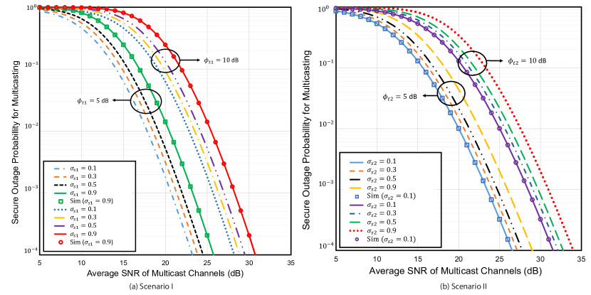
Figure 2: The SOPM versus average SNR of multicast channels varying $\sigma_{s1}$ and $\sigma_{s2}$ for selected values of $\phi_{t1}$ and $\phi_{t2}$ with $\mathcal{M}=\mathcal{N}=$ 2, $\mathcal{K}=4$, (a) $m_{m1}=m_{t1}=5$, $\mu_{p1}=\mu_{m1}=\mu_{t1}=0.5$ and $\eta_{p}=\eta_{m}=\eta_{t}=0.5$, and (b) $m_{m2}=m_{t2}=5$, $\mu_{p2}=\mu_{m2}=\mu_{t2}=0.5$, $\kappa_{p}=\kappa_{m}=\kappa_{t}=0.5$.

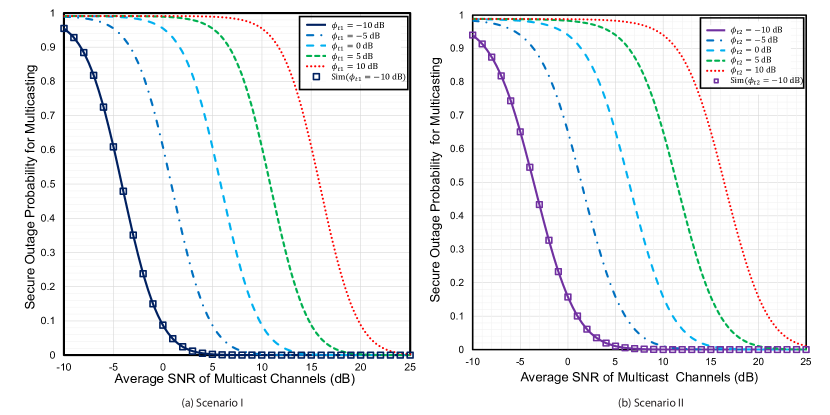
Figure 3: The SOPM versus average SNR of case-I and case-II multicast channels varying $\phi_{t1}$ and $\phi_{t2}$ with $\mathcal{M}=\mathcal{N}$=2, $\mathcal{K}=$ 2, (a) $m_{m1}=m_{t1}=5$, $\mu_{p1}=\mu_{m1}=\mu_{t1}=2$, $\eta_{p}=\eta_{m}=\eta_{t}=$ 0.5 and $\sigma_{s1}=0.5$ bits/s/Hz, and (b) $m_{m2}=m_{t2}=5$, $\mu_{p2}=\mu_{m2}=\mu_{t2}=2$, $\kappa_{p}=\kappa_{m}=\kappa_{t}=0.5$, $\sigma_{s2}=0.5$ bits/s/Hz.

In this section, we graphically represent the numerical results corresponding to the derived analytical expressions for the SOPM, PNSMC, and ESMC and observe how the system parameters, e.g., fading severity, shadowing, the number of relays, receivers, and eavesdroppers, etc. influence the multicast system’s secrecy characteristics. Analytical results are obtained using Mathematica software and for simulation purposes, we averaged $10^{6}$ random samples of each channel. Note that the infinite series in (6.2), (6.2), (7.2), (7.2), (8.2) and (8.2) converges quickly with a high level of accuracy just after fewer terms. Hence we assume the first 25 terms for each infinite series. Moreover, with a view to obtaining a clear comparison in terms of secrecy performance between the two considered scenarios, we present a set of curves corresponding to each scenario in each figure.

The SOPM is depicted as a function of the average SNR of the multicast channels in Figures 2a and 2b in order to observe the impacts due to variation in target secrecy rate. In each scenario, we assume two cases with $\phi_{t1}=\phi_{t2}=$ 5 dB and 10 dB. We can observe as seen from the figure that the SOPM increases with $\sigma_{s1}$ and $\sigma_{s2}$ which is also shown in [42]. Note that we assume a passive eavesdropping scenario in this work, hence the channel state information of eavesdropper networks is not known. For that reason, we assume a target secrecy rate and send information at this particular capacity. But if the instantaneous secrecy capacity falls below this target secure transmission capacity, then there will be a secrecy outage. Moreover, since the wireless channels are random in nature, an increase in target secrecy rate increases the probability of instantaneous secrecy rate falling below the target rate, hence the SOPM, as can be seen from the figure, will increase.

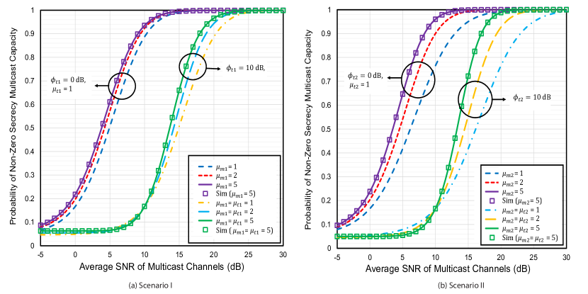
Figure 4: The PNSMC versus average SNR of multicast channels varying $\mu_{m1}$, $\mu_{t1}$, $\mu_{m2}$, $\mu_{t2}$ for selected values of $\phi_{t1}$= 0 dB, 5 dB, and $\phi_{t2}$= 0 dB, 5 dB with $\mathcal{M}=\mathcal{N}=$ 2, $\mathcal{K}=$ 2, (a) $m_{m1}=m_{t1}=5$, $\mu_{p1}=1$ and $\eta_{p}=\eta_{m}=\eta_{t}=$ 0.5, and (b) $m_{m2}=m_{t2}=5$, $\mu_{p2}=2$, and $\kappa_{p}=\kappa_{m}=\kappa_{t}=0.5$.

In Figures 3a and 3b, we illustrate the SOPM versus average SNR of the multicast channels showing the impacts of $\phi_{t1}$ and $\phi_{t2}$. It can be clearly seen from both the scenarios that the outage performance is better for lower values of the eavesdropper channel’s average SNR. It is obvious that the eavesdropper links becomes better due to an increased value of $\phi_{t1}$ and $\phi_{t2}$ which lets the eavesdroppers sneak more information from the multicast channels, and accordingly, the SOPM also increases. Same results also can be seen in [43, 44] which legibly justify our observations.

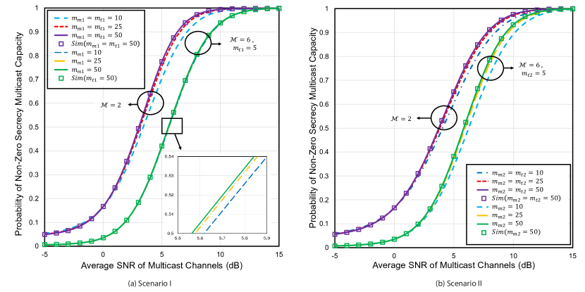
Figure 5: The PNSMC versus average SNR of multicast channels varying $m_{m1}$, $m_{t1}$, $m_{m2}$, and $m_{t2}$ for selected values of $\mathcal{M}$ with $\mathcal{N}=2$, $\mathcal{K}=2$, (a) $\phi_{t1}=$ 0 dB, $\mu_{p1}=\mu_{m1}=\mu_{t1}=$ 2, and $\eta_{p}=\eta_{m}=\eta_{t}=$ 0.5, and (b) $\phi_{t2}=$ 0 dB, $\mu_{p2}=\mu_{m2}=\mu_{t2}=$ 2, and $\kappa_{p}=\kappa_{m}=\kappa_{t}=$ 0.5.

The impacts of the number of multipath clusters of the multicast and the eavesdropper channels are depicted in Figures 4a and 4b in terms of PNSMC. It is observed that the PNSMC performance becomes better for the higher values of $\mu_{m1}$ and $\mu_{m2}$. The reason is that with the increase in the number of multipath clusters in the $\mathcal{K}\rightarrow\mathcal{M}$ link, the fading of the corresponding link is reduced. On the contrary, the lower amount of fading assists in improving the secrecy capacity, and thus the PNSMC performance also enhances as testified in [37]. Similarly, an increase in $\mu_{t_{1}}$ and $\mu_{t_{2}}$ reduce the fading of the $\mathcal{K}\rightarrow\mathcal{N}$ which will be beneficial for the eavesdroppers for wiretapping more confidential data. But if we simultaneously vary the shadowing severity of both the multicast and the eavesdropper links with equal values of $\mu_{m_{1}}$, $\mu_{m_{2}}$, $\mu_{t_{1}}$, and $\mu_{t_{2}}$, the PNSMC performance becomes better.

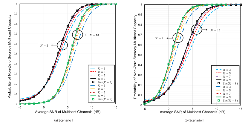
Figure 6: The PNSMC versus average SNR of multicast channels varying $\mathcal{K}$ for selected values of $\mathcal{N}$ with $\mathcal{M}=$ 2, (a) $\phi_{t1}=$ 0 dB, $m_{m1}=m_{t1}=$ 5, $\mu_{p1}=\mu_{m1}=\mu_{t1}=$ 2, and $\eta_{p}=\eta_{m}=\eta_{t}=$ 0.5, and (b) $\phi_{t2}=$ 0 dB, $m_{m2}=m_{t2}=$ 5, $\mu_{p2}=\mu_{m2}=\mu_{t2}=$ 2, and $\kappa_{p}=\kappa_{m}=\kappa_{t}=$ 0.5.

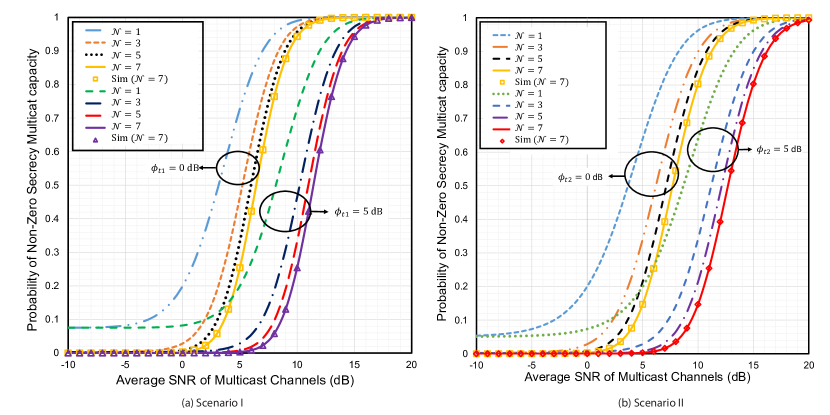
Figure 7: The PNSMC versus average SNR of multicast channels varying $\mathcal{N}$ for selected values of $\phi_{t1}$ and $\phi_{t2}$ with $\mathcal{M}=$ 4, $\mathcal{K}=$ 2, (a) $m_{m1}=m_{t1}=$ 5, $\mu_{p1}=\mu_{m1}=\mu_{t1}=$ 2, and $\eta_{p}=$$\eta_{m}=$$\eta_{t}=$ 0.5, and (b) $m_{m2}=m_{t2}=$ 5, $\mu_{p2}=\mu_{m2}=\mu_{t2}=$ 2, and $\kappa_{p}=\kappa_{m}=\kappa_{t}=$ 0.5.

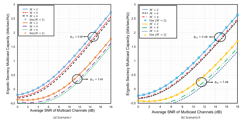
Figure 8: The ESMC versus average SNR of multicast channels varying $\mathcal{M}$ for selected values of $\phi_{t1}$ and $\phi_{t2}$ with $\mathcal{N}=$ 2, $\mathcal{K}=$ 4, (a) $m_{m1}=m_{t1}=$ 5, $\mu_{p1}=\mu_{m1}=\mu_{t1}=$ 2, $\eta_{p}=\eta_{m}=\eta_{t}=$ 0.5, $\sigma_{s1}$ = 0.5 bits/s/Hz, and (b) $m_{m2}=m_{t2}=$ 5, $\mu_{p2}=\mu_{m2}=\mu_{t2}=$ 2, $\kappa_{p}=\kappa_{m}=\kappa_{t}=$ 0.5, and $\sigma_{s2}$ = 0.5 bits/s/Hz.

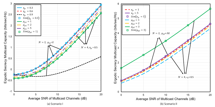
Figure 9: The ESMC versus average SNR of multicast channel varying $\eta_{p}$, $\mu_{p1}$, $\kappa_{p}$, and $\mu_{p2}$ for selected values of $\mathcal{N}$ with $\mathcal{M}$=2, $\mathcal{K}$=4, (a) $\phi_{t1}=$ 0 dB, $m_{m1}=m_{t1}=5$, $\mu_{m1}=\mu_{t1}=2$ , $\eta_{m}=\eta_{t}=0.5$ and $\sigma_{s1}=0.5$ bits/s/Hz, and (b) $\phi_{t2}=$ 0 dB, $m_{m2}=m_{t2}=5$, $\mu_{m2}=\mu_{t2}=2$, $\kappa_{m}=\kappa_{t}=0.5$, and $\sigma_{s2}=0.5$ bits/s/Hz.

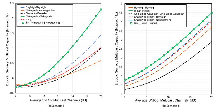
Figure 10: The ESMC versus average SNR of multicast channels for selected values of $\mu_{p1}$, $\mu_{m1}$, $\mu_{t1}$, $\mu_{p2}$, $\mu_{m2}$, $\mu_{t2}$, $\eta_{p}$, $\eta_{m}$, $\eta_{t}$, $\kappa_{p}$, $\kappa_{m}$, $\kappa_{t}$ with $\mathcal{M}=\mathcal{N}=\mathcal{K}=2$, (a) $m_{m1}=m_{t1}=35$, $\phi_{t1}=$ 0 dB, and $\sigma_{s1}=0.5$ bits/s/Hz, (b) $m_{m2}=m_{t2}=$ 35, $\phi_{t2}=$ 0 dB, and $\sigma_{s2}=0.5$ bits/s/Hz.

Figures 5a and 5b show the impacts of shadowing severity of multicast and eavesdropper channels on the physical layer security performance. We consider two groups with $\mathcal{M}$= 2, and 6. In the first group, we vary the shadowing severity of the $\mathcal{K}\rightarrow\mathcal{M}$ and $\mathcal{K}\rightarrow\mathcal{N}$ links simultaneously while in the second group we vary the severity of shadowing of the $\mathcal{K}\rightarrow\mathcal{M}$ links. It can clearly be observed that with the equally increasing values of $m_{m1}$ and $m_{t1}$, and $m_{m2}$ and $m_{t2}$, the secrecy performance is enhanced, and for increasing values of $m_{m1}$ and $m_{m2}$ individually, the performance also becomes better. This is because increasing $m_{m1}$ and $m_{m2}$ from 0 to $\infty$ indicates the shadowing severity changing from a stronger to weaker conditions while an increasing $m_{t1}$ and $m_{t2}$ reduces the shadowing severity of the eavesdropper links. The authors in [45] also observed some similar results as ours which is a clear indication that the results corresponding to our proposed dual-hop model are valid.

Figures 6a and 6b are depicted to explain the impacts of the number of relays on the PNSMC performance. We consider two cases with $\mathcal{N}=2$ and $\mathcal{N}=10$. The numerical results reveal that for both cases the proposed system exhibits an enhanced level of secrecy with the increasing number of relays $\mathcal{K}$. This result is also supported by [46]. An increased $\mathcal{K}$ represents an improved cooperative diversity and at the same time, the selection of the opportunistic channels in terms of best relaying ensures maximum capacity at the receive terminals thereby increasing the secrecy capacity.

In Figures 7a and 7b, the PNSMC is shown against the average SNR of multicast channels. The effects of the number of eavesdroppers $\mathcal{N}$ are shown assuming two groups with $\phi_{t1}=\phi_{t2}=$ 0 dB and 5 dB. As we consider maximum impacts of the eavesdroppers (maximum SNR at the eavesdropper) among $\mathcal{N}$ eavesdroppers (i.e. the worst case), it is evident that an increase in $\mathcal{N}$ will increase the probability of the existence of a strong eavesdropper channel in the system and hence the system’s security will be degraded as testified in [43].

To demonstrate the effects of the number of multicast receivers in the proposed model, we depict Figures 8a and 8b by showing ESMC against the average SNR of multicast channels. It can be observed that the secrecy capacity deteriorates with the number of receivers. Note that in wireless multicasting, a specific bandwidth is allocated for a group of multicast receivers which is divided among them equally according to the multicast scheme. With the increase in numbers of multicast receivers within the same allocated bandwidth, the bandwidth per receiver is reduced. Hence the SNR and capacity at the receiver’s terminals are also degraded which leads to a deteriorated secrecy performance as shown in [45].

In Figures 9a and 9b, the impacts of the shape parameters of the first-hop are depicted by showing ESMC against the average SNR of the multicast channels. We can observe that the ESMC decreases with $\eta_{p}$, but increases with $\mu_{p_{1}}$, $\mu_{p_{2}}$, and $\kappa_{p}$. The authors of [47, 26] also obtained similar results that clearly verify our analysis.

Generalization of the Existing Works:

It is noteworthy that the $\kappa-\mu$/IG and $\eta-\mu$/IG models exhibits extreme versatility as generalized $\kappa-\mu$ and $\eta-\mu$ models are the special cases of those IG models. Moreover, $\kappa-\mu$ and $\eta-\mu$ models also unify the performance evaluation of some classical multipath models. In the IG models, only the shadowing parameters (i.e. $m_{m1}$, $m_{t1}$, $m_{m2}$, and $m_{t2}$) determine the amount of shadowing of the mean signal power. If $m_{m1}$, $m_{t1}$, $m_{m2}$, and $m_{t2}$ $\rightarrow\infty$, then we can assume that both the dominant and scattered components suffer from severe shadowing. On the other hand, if $m_{m1}$, $m_{t1}$, $m_{m2}$, and $m_{t2}$ $\rightarrow 0$, then no shadowing is observed in the channels and hence the mean signal power can be considered to be the deterministic one. For that particular case, $\kappa-\mu$/IG and $\eta-\mu$/IG models takes the form of $\kappa-\mu$ and $\eta-\mu$ fading models, respectively.

In Figure 10a and 10b the generic nature of the proposed scenarios has been shown. For $\eta-\mu$ fading channel, setting $\eta_{p}$ = $\eta_{m}$ = $\eta_{t}$ = 0.9 and $\mu_{p1}$ = $\mu_{m1}$ = $\mu_{t1}$ = 1 with $m_{m1}$, $m_{t1}$, $m_{m2}$, and $m_{t2}$ $\rightarrow\infty$, we can obtain Nakagami-$m$ channel where $\mu_{m1}$, $\mu_{m2}$, $\mu_{t1}$, and $\mu_{t2}$ becomes equivalent to the Nakagami fading parameter $m$. Based on this, letting $\mu_{m1}$, $\mu_{m2}$, $\mu_{t1}$, and $\mu_{t2}$ equal to 1, we get Rayleigh distribution. Similarly, Gaussian channels can be obtained with $\eta_{p}$ = $\eta_{m}$ = $\eta_{t}$ = 0.9 and $\mu_{p1}$ = $\mu_{m1}$ = $\mu_{t1}$ = 0.25, and Nakagami-$q$ fading channel can be obtained with $\eta_{p}$ = $\eta_{m}$ = $\eta_{t}$ = 0.25 and $\mu_{p1}$ = $\mu_{m1}$ = $\mu_{t1}$ = 0.5. In the case of $\kappa-\mu$ model, we can generate Rician fading channel letting $\kappa_{p}$ = $\kappa_{m}$ = $\kappa_{t}$ = 5.4, $\mu_{p2}$ = $\mu_{m2}$ = $\mu_{t2}$ = 0.9, where $\kappa_{p}$, $\kappa_{m}$, and $\kappa_{t}$ become equivalent to the Rician-$K$ factor. Following those conditions, Rayleigh fading is obtained setting $\kappa_{p}$ = $\kappa_{m}$ = $\kappa_{t}$ = 0. Nakagami-$m$ is generated considering $\kappa_{p}$ = $\kappa_{m}$ = $\kappa_{t}$ = 0.001 and $\mu_{p2}$ = $\mu_{m2}$ = $\mu_{t2}$ = 1.5, where $\mu_{p2}$, $\mu_{m2}$ and $\mu_{t2}$ is equivalent to Nakagami fading parameter $m$. Likewise, we can obtain one-sided Gaussian channel setting $\kappa_{p}$ = $\kappa_{m}$ = $\kappa_{t}$ = 0 and $\mu_{p2}$ = $\mu_{m2}$ = $\mu_{t2}$ = 0.5, and shadowed Rician with $\kappa_{p}$ = $\kappa_{m}$ = $\kappa_{t}$ = 6 , $\mu_{p2}$ = $\mu_{m2}$ = $\mu_{t2}$ = 1. Besides the proposed scenarios also provide a good match to the secure shadowed Rician- Rayleigh [48, 49], and shadowed Rician- Nakagami-$m$ [50, 51] models. Hence, it can clearly be seen from the figures that the proposed scenarios (I and II) exhibits enormous versatility than any dual-hop multicast networks of the literature since a wide range of classical dual-hop multicast and broadcast models can be shown as special cases of the proposed work.

11 CONCLUSION

This work focuses on the secrecy analysis of dual-hop multicast communication systems in the presence of multiple eavesdroppers exploiting the best relay selection scheme. With a view to observing the impacts of each system parameter, we derive expressions for SOPM, PNSMC, and ESMC in closed-form which are further authenticated via Monte-Carlo simulations. It can clearly be seen from the numerical results that although fading, shadowing (both LOS and multiplicative), number of multicast receivers and eavesdroppers impose detrimental impacts on the secrecy performance, an acceptable secrecy level can till be maintained by first increasing the number of relays and then exploiting the best relay selection strategy. Moreover, the proposed model provides immense versatility since it can approximate a wide range of composite/multipath fading models of the literature. In future, our plan is to analyse the secrecy performance of multi-hop-multicast networks over IG composite fading models incorporating asymptotic analysis at high SNR regime.

12 Proof of Dual-hop SNRs (Scenario I)

12.1 $\mathcal{S}\rightarrow\mathcal{k}\rightarrow\mathcal{M}$ link

The PDF of $\Upsilon_{sm,1}$ and $\Upsilon_{st,1}$ is defined as [52]

$$f_{sm,1}(\Upsilon) =\frac{dF_{sm,1}(\Upsilon)}{d\Upsilon},$$ (41)

$$f_{st,1}(\Upsilon) =\frac{dF_{st,1}(\Upsilon)}{d\Upsilon},$$ (42)

where $F_{sm,1}(\Upsilon)$ and $F_{st,1}(\Upsilon)$ denote the CDFs of $\Upsilon_{sm,1}$ and $\Upsilon_{st,1}$. Now, the CDF of $\Upsilon_{sm,1}$ is defined as [53, eq. 12]

$$F_{sm,1}(\Upsilon) =1-\Pr(\Upsilon_{sp,1}>\Upsilon)\Pr(\Upsilon_{pm,1}>\Upsilon),$$ (43)

where $\Pr(\Upsilon_{sp,1}>\Upsilon_{sm,1})$ and $\Pr(\Upsilon_{pm,1}>\Upsilon_{sm,1})$ are the complementary cumulative distribution functions (CCDFs) of $\Upsilon_{sp,1}$ and $\Upsilon_{pm,1}$, and the CCDFs are, respectively defined by [54]

$$\Pr(\Upsilon_{sp,1}>\Upsilon_{sm,1}) =\int_{\Upsilon_{sm,1}}^{\infty}f_{sp,1}(\Upsilon)d\Upsilon,$$ (44)

$$\Pr(\Upsilon_{pm,1}>\Upsilon_{sm,1}) =\int_{\Upsilon_{sm,1}}^{\infty}f_{pm,1}(\Upsilon)d\Upsilon.$$ (45)

Substituting (2) into (44) and performing integration using [39, eq  3.351.2], we have

$$\Pr(\Upsilon_{sp,1}>\Upsilon_{sm,1}) =\sum_{n_{1}=0}^{\infty}\frac{\alpha_{2}}{\beta_{s}^{2\mu_{p1}+2n_{1}}}$$

$$\times\Gamma(2\mu_{p1}+2n_{1},\beta_{s}\Upsilon_{sm,1}).$$ (46)

Again substituting (4) into (45) and executing integration using [39, eq 3.194.2], we obtain

$$\Pr(\Upsilon_{pm,1}>\Upsilon_{sm,1})=\sum_{r_{1}=0}^{\infty}\frac{\lambda_{2}\Upsilon_{sm,1}^{-m_{m1}}}{\beta_{m}^{m_{m1}+2\mu_{m1}+2r_{1}}m_{m1}}$$

$$\times\,_{2}F_{1}\left(m_{m1}+2\mu_{m1}+2r_{1},m_{m1};m_{m1}+1;\frac{-1}{\beta_{m}\Upsilon_{sm,1}}\right)$$

$$=\sum_{r_{2}=0}^{\infty}\sum_{r_{1}=0}^{\infty}\frac{\lambda_{2}\Upsilon_{sm,1}^{-m_{m1}}}{\beta_{m}^{m_{m1}+2\mu_{m1}+2r_{1}}m_{m1}}$$

$$\times\frac{\left(m_{m1}\right)_{r_{2}}\left(m_{m1}+2\mu_{m1}+2r_{1}\right)_{r_{2}}}{r_{2}!\left(m_{m1}+1\right)_{r_{2}}\left(-\beta_{m}\right)^{r_{2}}}.$$ (47)

After a few terms, the infinite series here quickly converges. [55]. Now, substituting (12.1) and (12.1) into (43), the CDF of $\Upsilon_{sm,1}$ is obtained as

$$F_{sm,1}(\Upsilon) =1-\sum_{r_{2}=0}^{\infty}\sum_{r_{1}=0}^{\infty}\sum_{n_{1}=0}^{\infty}\Lambda_{2}\Upsilon^{-m_{m1}-r_{2}}$$

$$\times\Gamma(2\mu_{p1}+2n_{1},\beta_{s}\Upsilon),$$ (48)

where $\Lambda_{2}=\frac{\Lambda_{1}\left(m_{m1}\right)_{r_{2}}\left(m_{m1}+2\mu_{m1}+2r_{1}\right)_{r_{2}}}{r_{2}!\left(m_{m1}+1\right)_{r_{2}}\left(-\beta_{m}\right)^{r_{2}}}$, and
$\Lambda_{1}=\frac{\alpha_{2}\lambda_{2}\beta_{s}^{-2\mu_{p1}-2n_{1}}}{\beta_{m}^{m_{m1}+2\mu_{m1}+2r_{1}}m_{m1}}$. Substituting (12.1) into (41) and performing differentiation with respect to $\Upsilon_{sm,1}$, the PDF of $\Upsilon_{sm,1}$ is obtained in (3.2).

12.2 $\mathcal{S}\rightarrow\mathcal{k}\rightarrow\mathcal{N}$ link

Similar to (12.1), the CDF of $\Upsilon_{st,1}$ is given by

$$F_{st,1}(\Upsilon) =1-\sum_{\nu_{2}=0}^{\infty}\sum_{\nu_{1}=0}^{\infty}\sum_{n_{1}=0}^{\infty}\chi_{2}\Upsilon^{-m_{t1}-\nu_{2}}$$

$$\times\Gamma(2\mu_{p1}+2n_{1},\beta_{s}\Upsilon),$$ (49)

where $\chi_{2}=\frac{\chi_{1}\left(m_{t1}\right)_{\nu_{2}}\left(m_{t1}+2\mu_{t1}+2\nu_{1}\right)_{\nu_{2}}}{\nu_{2}!\left(m_{t1}+1\right)_{\nu_{2}}\left(-\beta_{e}\right)^{\nu_{2}}}$, and $\chi_{1}=\frac{\xi_{2}\beta_{s}^{-2\mu_{p1}-2n_{1}}}{\beta_{e}^{m_{t1}+2\mu_{t1}+2\nu_{1}}m_{t1}}$, Substituting (12.2) into (42) and performing differentiation with respect to $\Upsilon_{st,1}$, the PDF of $\Upsilon_{st,1}$ is obtained as shown in (3.2).

13 Proof of Best Relay Selection (Scenario I)

13.1 $\mathcal{S}\rightarrow\mathcal{k}\rightarrow\mathcal{M}$ link

Mathematically, the CDF of $\Upsilon_{bm,1}$ is defined as

$$F_{bm,1}(\Upsilon)=[F_{sm,1}(\Upsilon)]^{\mathcal{K}}.$$ (50)

Substituting (12.1) into (50), the CDF of $\Upsilon_{bm,1}$ is obtained as

$$F_{bm,1}(\Upsilon)= \biggl{[}1-\sum_{r_{2}=0}^{\infty}\sum_{r_{1}=0}^{\infty}\sum_{n_{1}=0}^{\infty}\Lambda_{2}\Upsilon^{-m_{m1}-r_{2}}$$

$$\times\Gamma(2\mu_{p1}+2n_{1},\beta_{s}\Upsilon)\biggl{]}^{\mathcal{K}}.$$ (51)

Differentiating (50) with respect to $\Upsilon_{sm,1}$, we get the PDF of $\Upsilon_{bm,1}$ as

$$f_{bm,1}(\Upsilon) =\mathcal{K}f_{sm,1}(\Upsilon)[F_{sm,1}(\Upsilon)]^{\mathcal{K}-1}.$$ (52)

Substituting (12.1) and (3.2) into (52), we obtain (3.3).

13.2 $\mathcal{S}\rightarrow\mathcal{k}\rightarrow\mathcal{N}$ link

Similar to (13.1), the CDF of $\Upsilon_{bt,1}$ is given by

$$F_{bt,1}(\Upsilon)= \biggl{[}1-\sum_{\nu_{2}=0}^{\infty}\sum_{\nu_{1}=0}^{\infty}\sum_{n_{1}=0}^{\infty}\chi_{2}\Upsilon^{-m_{t1}-\nu_{2}}$$

$$\times\Gamma(2\mu_{p1}+2n_{1},\beta_{s}\Upsilon)\biggl{]}^{\mathcal{K}}.$$ (53)

Differentiating (13.2) with respect to $\Upsilon_{st,1}$, the PDF of $\Upsilon_{bt,1}$ can be obtained that is given by (3.3).

14 Proof of Dual-hop SNRs (Scenario II)

14.1 $\mathcal{S}\rightarrow\mathcal{k}\rightarrow\mathcal{M}$ link

Denoting $\Upsilon_{sm,2}$, and $\Upsilon_{st,2}$ as the SNRs of $\mathcal{S}\rightarrow\mathcal{K}\rightarrow\mathcal{M}$, and $\mathcal{S}\rightarrow\mathcal{K}\rightarrow\mathcal{N}$ links, respectively, the PDFs of $\Upsilon_{sm,2}$ and $\Upsilon_{st,2}$ are given by

$$f_{sm,2}(\Upsilon)=\frac{dF_{sm,2}(\Upsilon)}{d\Upsilon},$$ (54)

$$f_{st,2}(\Upsilon)=\frac{dF_{st,2}(\Upsilon)}{d\Upsilon},$$ (55)

where $F_{sm,2}(\Upsilon)$ and $F_{st,2}(\Upsilon)$ denote the CDFs of $\Upsilon_{sm,2}$ and $\Upsilon_{st,2}$. Similar to (43), the CDF of $\Upsilon_{sm,2}$ is defined by

$$F_{sm,2}(\Upsilon)=1-\Pr(\Upsilon_{sp,2}>\Upsilon)\Pr(\Upsilon_{pm,2}>\Upsilon),$$ (56)

where $\Pr(\Upsilon_{sp,2}>\Upsilon_{sm,2})$ and $\Pr(\Upsilon_{pm,2}>\Upsilon_{sm,2})$ are the complementary cumulative distribution functions (CCDFs) of $\Upsilon_{sp,2}$ and $\Upsilon_{pm,2}$ which are, respectively defined by

$$\Pr(\Upsilon_{sp,2}>\Upsilon_{sm,2})=\int_{\Upsilon_{sm,2}}^{\infty}f_{sp,2}(\Upsilon)d\Upsilon,$$ (57)

$$\Pr(\Upsilon_{pm,2}>\Upsilon_{sm,2})=\int_{\Upsilon_{sm,2}}^{\infty}f_{pm,2}(\Upsilon)d\Upsilon.$$ (58)

Substituting (13) into (57) and performing integration using [39, eq.  3.351.2], we get

$$\Pr(\Upsilon_{sp,2}>\Upsilon_{sm,2}) =\sum_{\rho_{1}=0}^{\infty}\delta_{2}\delta_{b_{1}}^{-\mu_{p2}-\rho_{1}}$$

$$\times\Gamma(\mu_{p2}+\rho_{1},\delta_{b_{1}}\Upsilon_{sm,2}),$$ (59)

where $\delta_{b_{1}}=\frac{\mu_{p2}(1+\kappa_{p})}{\phi_{p2}}$. Again substituting (15) into (58) and performing integration, we get

$$\Pr(\Upsilon_{pm,2}>\Upsilon_{sm,2})=\sum_{\rho_{2}=0}^{\infty}\frac{\delta_{5}\Upsilon_{sm,2}^{-m_{m2}}}{\delta_{4}^{m_{m2}+\mu_{m}2+\rho_{2}}m_{m2}}$$

$$\times\,_{2}F_{1}\left(m_{m2}+\mu_{m2}+\rho_{2},m_{m2};m_{m2}+1;\frac{-1}{\delta_{4}\Upsilon_{sm,2}}\right)$$

$$=\sum_{\rho_{3}=0}^{\infty}\sum_{\rho_{2}=0}^{\infty}\frac{\delta_{5}\Upsilon_{sm,2}^{-m_{m2}}}{\delta_{4}^{m_{m2}+\mu_{m}2+\rho_{2}}m_{m2}}$$

$$\times\frac{\left(m_{m2}+\mu_{m2}+\rho_{2}\right)_{\rho_{3}}\left(m_{m2}\right)_{\rho_{3}}}{(-\delta_{4})^{\rho_{3}}\rho_{3}!\left(m_{m2}+1\right)_{\rho_{3}}}.$$ (60)

Where the infinite series converges rapidly as described in [28]. Substituting (14.1), and (14.1) into (56), the CDF of $\Upsilon_{sm,2}$ is obtained as

$$F_{sm,2}(\Upsilon) =1-\sum_{\rho_{3}=0}^{\infty}\sum_{\rho_{2}=0}^{\infty}\sum_{\rho_{1}=0}^{\infty}\delta_{7}\Upsilon^{-m_{m2}-\rho_{3}}$$

$$\times\Gamma(\mu_{p2}+\rho_{1},\delta_{b_{1}}\Upsilon),$$ (61)

where $\delta_{7}=\delta_{6}\frac{\left(m_{m2}+\mu_{m2}+\rho_{2}\right)_{\rho_{3}}\left(m_{m2}\right)_{\rho_{3}}}{(-\delta_{4})^{\rho_{3}}\rho_{3}!\left(m_{m2}+1\right)_{\rho_{3}}}$, and $\delta_{6}=\frac{\delta_{2}\delta_{5}\delta_{b_{1}}^{-\mu_{p2}-\rho_{1}}}{\delta_{4}^{m_{m2}+\mu_{m2}+\rho_{2}}m_{m2}}$. Substituting (14.1) into (54) and performing differentiation with respect to $\Upsilon_{sm,2}$, the PDF of $\Upsilon_{sm,2}$ is obtained in (4.2).

14.2 $\mathcal{S}\rightarrow\mathcal{k}\rightarrow\mathcal{N}$ link

Similar to (14.1), the CDF of $\Upsilon_{st,2}$ is given by

$$F_{st,2}(\Upsilon) =1-\sum_{\sigma_{2}=0}^{\infty}\sum_{\rho_{1}=0}^{\infty}\sum_{\sigma_{3}=0}^{\infty}\beta_{7}\Upsilon^{-m_{t2}-\sigma_{3}}$$

$$\times\Gamma(\mu_{p2}+\rho_{1},\delta_{b_{1}}\Upsilon),$$ (62)

where $\beta_{7}=\beta_{6}\frac{\left(m_{t2}+\mu_{t2}+\sigma_{2}\right)_{\sigma_{3}}\left(m_{t2}\right)_{\sigma_{3}}}{(-\beta_{2})^{\sigma_{3}}\sigma_{3}!\left(m_{t2}+1\right)_{\sigma_{3}}}$, and $\beta_{6}=\frac{\delta_{2}\beta_{3}\delta_{b_{1}}^{-\mu_{p2}-\sigma_{1}}}{\beta_{2}^{m_{t2}+\mu_{t2}+\sigma_{2}}m_{t2}}$. Now, substituting (14.2) into (55) and performing differentiation with respect to $\Upsilon_{st,2}$, we obtain (4.2).

15 Proof of Best Relay Selection (Scenario II)

15.1 $\mathcal{S}\rightarrow\mathcal{k}\rightarrow\mathcal{M}$ link

The CDF of $\Upsilon_{bm,2}$ is defined as

$$F_{bm,2}(\Upsilon)=[F_{sm,2}(\Upsilon)]^{\mathcal{K}}.$$ (63)

Now, substituting (14.1) into (63), the CDF of $\Upsilon_{bm,2}$ is obtained as

$$F_{bm,2}(\Upsilon)= [1-\sum_{\rho_{3}=0}^{\infty}\sum_{\rho_{2}=0}^{\infty}\sum_{\rho_{1}=0}^{\infty}\delta_{7}\Upsilon_{sm,2}^{-m_{m2}-\rho_{3}}$$

$$\times\Gamma(\mu_{p2}+\rho_{1},\delta_{b_{1}}\Upsilon_{sm,2})]^{\mathcal{K}}.$$ (64)

Differentiating (63) with respect to $\Upsilon_{sm,2}$, we get the PDF of $\Upsilon_{bm,2}$ as

$$f_{bm,2}(\Upsilon)=\mathcal{K}f_{sm,2}(\Upsilon)[F_{sm,2}(\Upsilon)]^{\mathcal{K}-1}.$$ (65)

Now substituing (14.1) , and (4.2) into (65), we get $f_{bm,2}(\Upsilon)$ as shown in (4.3).

15.2 $\mathcal{S}\rightarrow\mathcal{k}\rightarrow\mathcal{N}$ link

Similar to (15.1), the CDF of $\Upsilon_{bt,2}$ is given by

$$F_{bt,2}(\Upsilon) =[1-\sum_{\sigma_{3}=0}^{\infty}\sum_{\sigma_{2}=0}^{\infty}\sum_{\rho_{1}=0}^{\infty}\beta_{7}\Upsilon^{-m_{t2}-\sigma_{3}}$$

$$\times\Gamma(\mu_{p2}+\rho_{1},\delta_{b_{1}}\Upsilon)]^{\mathcal{K}}.$$ (66)

Differentiating (15.2) with respect to $\Upsilon_{st,2}$, the PDF of $\Upsilon_{bt,2}$ is shown in (4.3).

16 Proof of Multicast Channel Models

16.1 Scenario I

In the case of mixed $\eta-\mu$ and $\eta-\mu$ /IG composite fading channel, the PDF of $\sigma_{min,1}$ is given by

$$f_{\sigma_{min,1}}(\Upsilon)=\mathcal{M}f_{bm,1}(\Upsilon)[1-F_{bm,1}(\Upsilon)]^{\mathcal{M}-1}.$$ (67)

Plugging (13.1) and (3.3) into (67) leads to

$$f_{\sigma_{min,1}}(\Upsilon)=\sum_{r_{2}=0}^{\infty}\sum_{r_{1}=0}^{\infty}\sum_{n_{1}=0}^{\infty}\Lambda_{2}\mathcal{M}\mathcal{K}\biggl{[}e^{-\beta_{s}\Upsilon}$$

$$\times\Upsilon^{-n_{2}+2\mu_{p1}+2n_{1}}+\Upsilon^{-n_{2}}\Gamma(2\mu_{p1}+2n_{1},\beta_{s}\Upsilon)\biggl{]}$$

$$\times\biggl{[}1-\sum_{r_{2}=0}^{\infty}\sum_{r_{1}=0}^{\infty}\sum_{n_{1}=0}^{\infty}\Lambda_{2}\Upsilon^{-m_{m1}-r_{2}}\Gamma(2\mu_{p1}+2n_{1},\beta_{s}\Upsilon)\biggl{]}^{\mathcal{K}-1}$$

$$\times\biggl{[}1-\biggl{(}1-\sum_{r_{2}=0}^{\infty}\sum_{r_{1}=0}^{\infty}\sum_{n_{1}=0}^{\infty}\Lambda_{2}\Upsilon^{-m_{m1}-r_{2}}$$

$$\times\Gamma(2\mu_{p1}+2n_{1},\beta_{s}\Upsilon)\biggl{)}^{\mathcal{K}}\biggl{]}^{\mathcal{M}-1}.$$ (68)

Using binomial expansion of [39, eq  1.111], (16.1) can be expressed as

$$f_{\sigma_{min,1}}(\Upsilon)=\sum_{r_{5}=0}^{\mathcal{M}-1}\sum_{r_{6}=0}^{\mathcal{K}+\mathcal{K}r_{5}-1}\sum_{r_{2}=0}^{\infty}\sum_{r_{1}=0}^{\infty}\sum_{n_{1}=0}^{\infty}\mathcal{M}\mathcal{K}\Lambda_{6}\Lambda_{2}$$

$$\times\biggl{[}\Upsilon^{-n_{2}+2\mu_{p1}+2n_{1}}e^{-\beta_{s}\Upsilon}+\Upsilon^{-n_{2}}\Gamma(2\mu_{p1}+2n_{1},\beta_{s}\Upsilon)\biggl{]}$$

$$\times\biggl{[}\sum_{r_{1}=0}^{\infty}\sum_{n_{1}=0}^{\infty}\sum_{r_{2}=0}^{\infty}\Lambda_{2}\Upsilon^{-m_{m1}-r_{2}}\Gamma(2\mu_{p1}+2n_{1},\beta_{s}\Upsilon)\biggl{]}^{r_{6}},$$ (69)

where $\Lambda_{6}={(-1)^{r_{5}+r_{6}}}\binom{\mathcal{M}-1}{r_{5}}\binom{\mathcal{K}+\mathcal{K}r_{5}-1}{r_{6}}$. Making use of [39, eq  8.352.7], (16.1) can be further simplified as

$$f_{\sigma_{min,1}}(\Upsilon)=\sum_{r_{5}=0}^{\mathcal{M}-1}\sum_{r_{6}=0}^{\mathcal{K}+\mathcal{K}r_{5}-1}\sum_{r_{2}=0}^{\infty}\sum_{r_{1}=0}^{\infty}\sum_{n_{1}=0}^{\infty}\mathcal{M}\mathcal{K}\Lambda_{6}\Lambda_{2}$$

$$\times\biggl{[}\Upsilon^{-n_{2}+2\mu_{p1}+2n_{1}}+\sum_{r_{7}=0}^{2\mu_{p1}+2n_{1}-1}\Lambda_{7}\Upsilon^{-n_{2}+r_{7}}\biggl{]}$$

$$\times e^{-\beta_{s}\Upsilon}[\Theta_{1}(\Upsilon)]^{r_{6}},$$ (70)

where $\Lambda_{7}=\frac{\Gamma(2\mu_{p1}+2n_{1})}{r_{7}!\beta_{s}^{-r_{7}}}$. Here,

$$\Theta_{1}(\Upsilon)=\sum_{r_{8}=0}^{2\mu_{p1}+2n_{1}-1}\sum_{r_{2}=0}^{\infty}\sum_{r_{1}=0}^{\infty}\sum_{n_{1}=0}^{\infty}\Lambda_{8}\Upsilon^{-m_{m1}-r_{2}+r_{8}}e^{-\beta_{s}\Upsilon},$$ (71)

where $\Lambda_{8}=\frac{\Lambda_{2}\Gamma(2\mu_{p1}+2n_{1})}{r_{8}!\beta_{s}^{-r_{8}}}$. Using the multinomial theorem of [17, eq.  7], we get

$$[\Theta_{1}(\Upsilon)]^{r_{6}}=\Xi_{\psi_{r_{6}}}e^{-\phi_{\psi_{r_{6}}}\Upsilon}\Upsilon^{\varphi_{\psi_{r_{6}}}}$$

$$\times\sum_{\psi_{r_{6}}}\binom{r_{6}}{p_{0,0,0,0,\ldots,}p_{r_{8},r_{2},r_{1},n_{1},\ldots,}n_{2\mu_{p1}+2n_{1}-1,\infty,\infty,\infty}},$$ (72)

where $\binom{b}{b_{1},b_{2},...,b_{m}}=\frac{b!}{b_{1}!,b_{2}!,\ldots,b_{m}!}$ denotes the multinomial coefficients, $\Xi_{\psi_{r_{6}}}=\Pi_{r_{8},r_{2},r_{1},n_{1}}\Lambda_{8}^{p_{r_{8},r_{2},r_{1},n_{1}}}$, $\phi_{\psi_{r_{6}}}=\sum_{r_{8}}\sum_{r_{2}}\sum_{r_{1}}\sum_{n_{1}}\beta_{s}p_{r_{8},r_{2},r_{1},n_{1}}$, and $\varphi_{\psi_{r_{6}}}=\sum_{r_{8}}\sum_{r_{2}}\sum_{r_{1}}\sum_{n_{1}}(-m_{m1}-r_{2}+r_{8})p_{r_{8},r_{2},r_{1},n_{1}}$. The sum of (16.1) is to be carried out for each element of $\psi_{r_{6}}$, which is defined by

$$\psi_{r_{6}} =\{(p_{0,0,0,0,\ldots,}p_{r_{8},r_{2},r_{1},n_{1},\ldots,}n_{2\mu_{p1}+2n_{1}-1,\infty,\infty,\infty}):$$

$$p_{r_{8},r_{2},r_{1},n_{1}}\in N0\leqslant r_{8}\leqslant 2\mu_{p1}+2n_{1}-1,0\leqslant r_{2}\leqslant\infty,$$

$$0\leqslant r_{1}\leqslant\infty,0\leqslant n_{1}\leqslant\infty;\sum_{r_{8},r_{2},r_{1},n_{1}}p_{r_{8},r_{2},r_{1},n_{1}}=r_{6}\}.$$ (73)

After modifying (16.1), we get

$$[\Theta_{1}(\Upsilon)]^{r_{6}}=\sum_{\psi_{r_{6}}}\Lambda_{9}e^{-\phi_{\psi_{r_{6}}}\Upsilon}\Upsilon^{\varphi_{\psi_{r_{6}}}},$$ (74)

where $\Lambda_{9}=\binom{r_{6}}{p_{0,0,0,0,\ldots,}p_{r_{8},r_{2},r_{1},n_{1},\ldots,}n_{2\mu_{p1}+2n_{1}-1,\infty,\infty,\infty}}\Xi_{\psi_{r_{6}}}$. Substituting (74) into (16.1), we get the final expression of $f_{\sigma_{min,1}}(\Upsilon)$ in (5.1).

16.2 Scenario II

For the mixed $\kappa-\mu$ and $\kappa-\mu$ /IG composite fading channel, the PDF of $\sigma_{min,2}$ is given by

$$f_{\sigma_{min,2}}(\Upsilon)=\mathcal{M}f_{bm,2}(\Upsilon)[1-F_{bm,2}(\Upsilon)]^{\mathcal{M}-1}.$$ (75)

Substituting (15.1) and (4.3) into (75), we get

$$f_{\sigma_{min,2}}(\Upsilon)=\sum_{\rho_{3}=0}^{\infty}\sum_{\rho_{2}=0}^{\infty}\sum_{\rho_{1}=0}^{\infty}\delta_{7}\mathcal{M}\mathcal{K}\biggl{[}e^{-\Upsilon\delta_{b_{1}}}$$

$$\times\Upsilon^{-\rho_{3}-m_{m2}-1+\mu_{p2}+\rho_{1}}+\Upsilon^{-1-\rho_{3}-m_{m2}}$$

$$\times\Gamma[\mu_{p2}+\rho_{1},\Upsilon\delta_{b_{1}}]\biggl{]}$$

$$\times\biggl{[}1-\sum_{\rho_{2}=0}^{\infty}\sum_{\rho_{1}=0}^{\infty}\sum_{\rho_{3}=0}^{\infty}\delta_{7}\Upsilon^{-m_{m2}-\rho_{3}}\Gamma(\mu_{p2}+\rho_{1},\delta_{b_{1}}\Upsilon)\biggl{]}^{\mathcal{K}-1}$$

$$\times\biggl{[}1-\biggl{(}1-\sum_{\rho_{2}=0}^{\infty}\sum_{\rho_{1}=0}^{\infty}\sum_{\rho_{3}=0}^{\infty}\delta_{7}\Upsilon^{-m_{m2}-\rho_{3}}$$

$$\times\Gamma(\mu_{p2}+\rho_{1},\delta_{b_{1}}\Upsilon)\biggl{)}^{\mathcal{K}}\biggl{]}^{\mathcal{M}-1}.$$ (76)

Using [39, eq.  1.111], (16.2) can be simplified as

$$f_{\sigma_{min,2}}(\Upsilon)=\sum_{\rho_{6}=0}^{\mathcal{M}-1}\sum_{\rho_{7}=0}^{\mathcal{K}+\mathcal{K}\rho_{6}-1}\sum_{\rho_{2}=0}^{\infty}\sum_{\rho_{1}=0}^{\infty}\sum_{\rho_{3}=0}^{\infty}\mathcal{M}\mathcal{K}\delta_{10}\delta_{7}$$

$$\times\biggl{[}e^{-\Upsilon\delta_{b_{1}}}\Upsilon^{-\rho_{3}-m_{m2}-1+\mu_{p2}+\rho_{1}}$$

$$+\Upsilon^{-1-\rho_{3}-m_{m2}}\Gamma[\mu_{p2}+\rho_{1},\Upsilon\delta_{b_{1}}]\biggl{]}\times\biggl{[}\sum_{\rho_{2}=0}^{\infty}\sum_{\rho_{1}=0}^{\infty}$$

$$\times\sum_{\rho_{3}=0}^{\infty}\delta_{7}\Upsilon^{-m_{m2}-\rho_{3}}\Gamma(\mu_{p2}+\rho_{1},\delta_{b_{1}}\Upsilon)\biggl{]}^{\rho_{7}},$$ (77)

where $\delta_{10}=(-1)^{\rho_{6}+\rho_{7}}\binom{\mathcal{M}-1}{\rho_{6}}\binom{\mathcal{K}+\mathcal{K}\rho_{6}-1}{\rho_{7}}$. Again using [39, eq.  8.352.7], (16.2) can be further simplified as

$$f_{\sigma_{min,2}}(\Upsilon)=\sum_{\rho_{6}=0}^{\mathcal{M}-1}\sum_{\rho_{7}=0}^{\mathcal{K}+\mathcal{K}\rho_{6}-1}\sum_{\rho_{3}=0}^{\infty}\sum_{\rho_{2}=0}^{\infty}\sum_{\rho_{1}=0}^{\infty}\mathcal{M}\mathcal{K}\delta_{10}\delta_{7}$$

$$\times e^{-\Upsilon\delta_{b_{1}}}\biggl{[}\Upsilon^{\delta_{11}+\mu_{p2}+\rho_{1}}+\sum_{\rho_{8}=0}^{\mu_{p2}+\rho_{1}-1}\delta_{12}\Upsilon^{\delta_{11}+\rho_{8}}\biggl{]}$$

$$\times\biggl{[}\Theta_{2}(\Upsilon)\biggl{]}^{\rho_{7}},$$ (78)

where $\delta_{11}=-m_{m2}-\rho_{3}-1$ , $\delta_{11}+1=-m_{m2}-\rho_{3}$, and $\delta_{12}=\frac{\Gamma(\mu_{p2}+\rho_{1})}{(\rho_{8})!\delta_{b_{1}}^{-\rho_{8}}}$. Here

$$\Theta_{2}(\Upsilon)=\sum_{\rho_{9}=0}^{\mu_{p2}+\rho_{1}-1}\sum_{\rho_{3}=0}^{\infty}\sum_{\rho_{2}=0}^{\infty}\sum_{\rho_{1}=0}^{\infty}\delta_{13}\Upsilon^{\delta_{11}+\rho_{9}+1}e^{-\Upsilon\delta_{b_{1}}},$$ (79)

where $\delta_{13}=\frac{\delta_{7}\Gamma(\mu_{p2}+\rho_{1})}{\rho_{9}!(\delta_{b_{1}})^{-\rho_{9}}}$. Using the multinomial theorem of [17, eq.  7], we get

$$[\Theta_{2}(\Upsilon)]^{\rho_{7}}=\chi_{\psi_{\rho_{7}}}e^{-\Theta_{\psi_{\rho_{7}}}\Upsilon}\Upsilon^{\eta_{\psi_{\rho_{7}}}}$$

$$\times\sum_{\psi_{\rho_{7}}}\binom{\rho_{7}}{g_{0,0,0,0},\ldots,g_{\rho_{9},\rho_{3}\rho_{2},\rho_{1}},\ldots,n_{\mu_{p2}+\rho_{1}-1,\infty,\infty,\infty}},$$ (80)

where $\binom{a}{a_{1},a_{2},\ldots,a_{m}}=\frac{a!}{a_{1}!a_{2}!\ldots a_{m}!}$ denotes the multinomial coefficients, $\chi_{\psi_{\rho_{7}}}=\Pi_{\rho_{9},\rho_{3},\rho_{2},\rho_{1}}\delta_{13}^{g_{\rho_{9},\rho_{3},\rho_{2},\rho_{1}}}$, $\eta_{\psi_{\rho_{7}}}=\sum_{\rho_{9}}\sum_{\rho_{3}}\sum_{\rho_{2}}\sum_{\rho_{1}}^{(\delta_{11}+\rho_{9}+1){g_{\rho_{9},\rho_{3},\rho_{2},\rho_{1}}}}$ and $\Theta_{\psi_{\rho_{7}}}=\sum_{\rho_{9}}\sum_{\rho_{3}}\sum_{\rho_{2}}\sum_{\rho_{1}}\delta_{b_{1}}{g_{\rho_{9},\rho_{3},\rho_{2},\rho_{1}}}$. For each element of $\psi_{\rho_{7}}$, the sum in (16.2) is to be performed, which can be defined as

$$\psi_{\rho_{7}}= (g_{0,0,0,0},\ldots,g_{\rho_{9},\rho_{3}\rho_{2},\rho_{1}},\ldots,n_{\mu_{p2}+\rho_{1}-1,\infty,\infty,\infty}):$$

$$g_{\rho_{9},\rho_{3},\rho_{2},\rho_{1}}\in\mathbb{N}0\leq\rho_{9}\leq\mu_{p2}+\rho_{1}-1,0\leq\rho_{3}\leq\infty,$$

$$0\leq\rho_{2}\leq\infty,0\leq\rho_{1}\leq\infty;\sum_{\rho_{9},\rho_{3},\rho_{2},\rho_{1}}g_{\rho_{9},\rho_{3},\rho_{2},\rho_{1}}=\rho_{7}.$$ (81)

Substituting (16.2) into (16.2), we get the final expression of $f_{\sigma_{min,2}}(\Upsilon_{bm,2})$ in (5.2).

17 Proof of Eavesdropper Channel Models

17.1 Scenario I

The PDF of $\sigma_{max,1}$ in the case of mixed $\eta-\mu$ and $\eta-\mu$ /IG composite fading channel is given by

$$f_{\sigma_{max,1}}(\Upsilon)=\mathcal{N}f_{bt,1}(\Upsilon)[F_{bt,1}(\Upsilon)]^{\mathcal{N}-1}.$$ (82)

Substituting (13.2), and (3.3) into (82), we get

$$f_{\sigma_{max,1}}(\Upsilon)=\sum_{\nu_{1}=0}^{\infty}\sum_{n_{1}=0}^{\infty}\sum_{\nu_{2}=0}^{\infty}\chi_{2}\mathcal{N}\mathcal{K}\biggl{[}e^{-\beta_{s}\Upsilon}$$

$$\times\Upsilon^{-n_{3}+2\mu_{p1}+2n_{1}}+\Upsilon^{-n_{3}}\Gamma(2\mu_{p1}+2n_{1},\beta_{s}\Upsilon)\biggl{]}$$

$$\times\biggl{[}1-\sum_{\nu_{2}=0}^{\infty}\sum_{\nu_{1}=0}^{\infty}\sum_{n_{1}=0}^{\infty}\chi_{2}\Upsilon^{-m_{t1}-\nu_{2}}\Gamma(2\mu_{p1}+2n_{1},\beta_{s}\Upsilon)\biggl{]}^{\mathcal{K}-1}$$

$$\times\biggl{[}[1-\sum_{\nu_{2}=0}^{\infty}\sum_{\nu_{1}=0}^{\infty}\sum_{n_{1}=0}^{\infty}\chi_{2}\Upsilon^{-m_{t1}-\nu_{2}}$$

$$\times\Gamma(2\mu_{p1}+2n_{1},\beta_{s}\Upsilon)]^{\mathcal{K}}\biggl{]}^{\mathcal{N}-1}.$$ (83)

Simplifying (17.1), we get

$$f_{\sigma_{max,1}}(\Upsilon)=\sum_{\nu_{6}=0}^{\mathcal{K}\mathcal{N}-1}\sum_{\nu_{2}=0}^{\infty}\sum_{\nu_{1}=0}^{\infty}\sum_{n_{1}=0}^{\infty}\mathcal{N}\mathcal{K}\chi_{6}\chi_{2}e^{-\beta_{s}\Upsilon}$$

$$\times\biggl{[}\Upsilon^{-n_{3}+2\mu_{p1}+2n_{1}}+\sum_{\nu_{7}=0}^{2\mu_{p1}+2n_{1}-1}\chi_{7}\Upsilon^{-n_{3}+\nu_{7}}\biggl{]}$$

$$\times\biggl{[}\Theta_{3}(\Upsilon)\biggl{]}^{\nu_{6}},$$ (84)

where $\chi_{6}=\binom{\mathcal{K}\mathcal{N}-1}{\nu_{6}}(-1)^{\nu_{6}}$, and $\chi_{7}=\frac{\Gamma(2\mu_{p1}+2n_{1})}{\nu_{7}!\beta_{s}^{-\nu_{7}}}$. Here

$$\Theta_{3}(\Upsilon)=\sum_{\nu_{8}=0}^{2\mu_{p1}+2n_{1}-1}\sum_{\nu_{2}=0}^{\infty}\sum_{\nu_{1}=0}^{\infty}\sum_{n_{1}=0}^{\infty}\chi_{8}\Upsilon^{-m_{t1}-\nu_{2}+\nu_{8}}e^{-\beta_{s}\Upsilon},$$ (85)

where $\chi_{8}=\frac{\chi_{2}\Gamma(2\mu_{p1}+2n_{1})}{\nu_{8}!\beta_{s}^{-\nu_{8}}}$. Applying multinomial theorem of [17, eq.  7], we obtain

$$[\Theta_{3}(\Upsilon)]^{\nu_{6}}=\Xi_{\nu_{6}}e^{-\phi_{\nu_{6}}\Upsilon}\Upsilon^{\varphi_{\nu_{6}}}$$

$$\times\sum_{\psi_{\nu_{6}}}\binom{\nu_{6}}{q_{0,0,0,0,\ldots,}q_{\nu_{8},\nu_{2},\nu_{1},n_{1}.\ldots,}n_{2\mu_{p1}+2n_{1}-1,\infty,\infty,\infty}},$$ (86)

where $\Xi_{\psi_{\nu_{6}}}=\Pi_{\nu_{8},\nu_{2},\nu_{1},n_{1}}\chi_{8}^{q_{\nu_{8},\nu_{2},\nu_{1},n_{1}}}$, $\phi_{\psi_{\nu_{6}}}=\sum_{\nu_{8}}\sum_{\nu_{2}}\sum_{\nu_{1}}\sum_{n_{1}}\beta_{s}q_{\nu_{8},\nu_{2},\nu_{1},n_{1}}$,and
$\varphi_{\psi_{\nu_{6}}}=\sum_{\nu_{8}}\sum_{\nu_{2}}\sum_{\nu_{1}}\sum_{n_{1}}(-m_{t1}-\nu_{2}+\nu_{8})q_{\nu_{8},\nu_{2},\nu_{1},n_{1}}$. Substituting (17.1) into (17.1), we get we get the final expression of $f_{\sigma_{max,1}}(\Upsilon)$ in (6.1).

17.2 Scenario II

In the case of mixed $\kappa-\mu$ and $\kappa-\mu$ /IG composite fading channel, the PDF of $\sigma_{max,2}$ is given by

$$f_{\sigma_{max}}(\Upsilon)=\mathcal{N}f_{bt,2}(\Upsilon)[F_{bt,2}(\Upsilon)]^{\mathcal{N}-1}.$$ (87)

Substituting (15.2) and (4.3) into (87), we get

$$f_{\sigma_{max,2}}(\Upsilon)=\sum_{\sigma_{3}=0}^{\infty}\sum_{\sigma_{2}=0}^{\infty}\sum_{\rho_{1}=0}^{\infty}\beta_{7}\mathcal{N}\mathcal{K}\biggl{[}e^{-\Upsilon\delta_{b_{1}}}$$

$$\times\Upsilon^{-\sigma_{3}-m_{t2}-1+\mu_{p2}+\sigma_{1}}+\Upsilon^{-1-\sigma_{3}-m_{t2}}$$

$$\times\Gamma[\mu_{p2}+\rho_{1},\Upsilon\delta_{b_{1}}]\biggl{]}$$

$$\times\biggl{[}1-\sum_{\sigma_{3}=0}^{\infty}\sum_{\sigma_{2}=0}^{\infty}\sum_{\rho_{1}=0}^{\infty}\beta_{7}\Upsilon^{-m_{t2}-\sigma_{3}}\Gamma(\mu_{p2}+\rho_{1},\delta_{b_{1}}\Upsilon)\biggl{]}^{\mathcal{K}-1}$$

$$\times\biggl{[}[1-\sum_{\sigma_{3}=0}^{\infty}\sum_{\sigma_{2}=0}^{\infty}\sum_{\rho_{1}=0}^{\infty}\beta_{7}\Upsilon^{-m_{t2}-\sigma_{3}}$$

$$\times\Gamma(\mu_{p2}+\rho_{1},\delta_{b_{1}}\Upsilon)]^{\mathcal{K}}\biggl{]}^{\mathcal{N}-1}.$$ (88)

Simplifying (17.2), we get

$$f_{\sigma_{max,2}}(\Upsilon)=\sum_{\sigma_{10}=0}^{\mathcal{K}\mathcal{N}-1}\sum_{\sigma_{3}=0}^{\infty}\sum_{\sigma_{2}=0}^{\infty}\sum_{\rho_{1}=0}^{\infty}\mathcal{N}\mathcal{K}\beta_{15}\beta_{7}e^{-\Upsilon\delta_{b_{1}}}$$

$$\times\biggl{[}\Upsilon^{\beta_{10}+\mu_{p2}+\rho_{1}}+\sum_{\sigma_{11}=0}^{\mu_{p2}+\rho_{1}-1}\beta_{16}\Upsilon^{\beta_{10}+\sigma_{11}}\biggl{]}$$

$$\times\biggl{[}\Theta_{4}(\Upsilon)\biggl{]}^{\sigma_{10}},$$ (89)

where $\beta_{10}=-m_{t2}-\sigma_{3}-1$, $\beta_{10}+1=-m_{t2}-\sigma_{3}$, $\beta_{15}=\binom{\mathcal{K}\mathcal{N}-1}{\sigma_{10}}(-1)^{\sigma_{10}}$, and $\beta_{16}=\frac{\Gamma(\mu_{p2}+\rho_{1})}{(\sigma_{11})!\delta_{b_{1}}^{-\sigma_{11}}}$. Here

$$\theta_{4}(\Upsilon)=\sum_{\sigma_{12}=0}^{\mu_{p2}+\rho_{1}-1}\sum_{\sigma_{3}=0}^{\infty}\sum_{\sigma_{2}=0}^{\infty}\sum_{\rho_{1}=0}^{\infty}\beta_{17}\Upsilon^{\beta_{10}+\sigma_{12}+1}e^{-\Upsilon\delta_{b_{1}}},$$ (90)

where $\beta_{17}=\frac{\beta_{7}\Gamma(\mu_{p2}+\rho_{1})}{\sigma_{12}!(\delta_{b_{1}})^{-\sigma_{12}}}$. Using the multinomial theorem of [17, eq.  7], we get

$$[\Theta_{4}(\Upsilon)]^{\sigma_{10}}=\chi_{\psi_{\sigma_{10}}}e^{-\Theta_{\psi_{\sigma_{10}}}\Upsilon}\Upsilon^{\eta_{\psi_{\sigma_{10}}}}$$

$$\times\sum_{\psi_{\sigma_{10}}}\binom{\sigma_{10}}{f_{0,0,0,0},\ldots,f_{\sigma_{12},\sigma_{3},\sigma_{2},\rho_{1}},\ldots,n_{\mu+\rho_{1}-1,\infty,\infty,\infty}},$$ (91)

where $\chi_{\psi_{\sigma_{10}}}=\Pi_{\sigma_{12},\sigma_{3},\sigma_{2},\rho_{1}}\beta_{17}^{f_{\sigma_{12},\sigma_{3},\sigma_{2},\rho_{1}}}$, $\eta_{\psi_{\sigma_{10}}}=\sum_{\sigma_{12}}\sum_{\sigma_{3}}\sum_{\sigma_{1}}\sum_{\rho_{1}}(\beta_{10}+\sigma_{12}+1){f_{\sigma_{12},\sigma_{3},\sigma_{2},\rho_{1}}}$, and $\Theta_{\psi_{\sigma_{10}}}=\sum_{\sigma_{12}}\sum_{\sigma_{3}}\sum_{\sigma_{2}}\sum_{\rho_{1}}\delta_{b_{1}}{f_{\sigma_{12},\sigma_{3},\sigma_{2},\rho_{1}}}$. Substituting (17.2) into (17.2), we get the final expression of $f_{\sigma_{max,2}}(\Upsilon)$ in (6.2).

References

• [1] L. Lv, F. Zhou, J. Chen, and N. Al-Dhahir, “Secure Cooperative Communications With an Untrusted Relay: A NOMA-Inspired Jamming and Relaying Approach,” IEEE Transactions on Information Forensics and Security, vol. 14, no. 12, pp. 3191–3205, 2019.
• [2] J. M. Moualeu, D. B. da Costa, W. Hamouda, U. S. Dias, and R. A. de Souza, “Physical Layer Security Over $\alpha$-$\kappa$-$\mu$ and $\alpha$-$\eta$-$\mu$ Fading Channels,” IEEE Transactions on Vehicular Technology, vol. 68, no. 1, pp. 1025–1029, 2018.
• [3] E. Diamanti, H.-K. Lo, B. Qi, and Z. Yuan, “Practical challenges in quantum key distribution,” npj Quantum Information, vol. 2, no. 1, pp. 1–12, 2016.
• [4] S. K. Yoo, N. Bhargav, S. L. Cotton, P. C. Sofotasios, M. Matthaiou, M. Valkama, and G. K. Karagiannidis, “The $\kappa$-$\mu$/inverse gamma and $\eta$-$\mu$/inverse gamma composite fading models: Fundamental statistics and empirical validation,” IEEE Trans. Commun., vol. 69, no. 8, pp. 5514–5530, 2017.
• [5] M. Bhatt and S. K. Soni, “ASEP Analysis Over Unified Lognormal Shadowed $\alpha$ $\eta$ $\mu$ and $\alpha$ $\kappa$ $\mu$ Composite Fading Channels,” in 2018 Second International Conference on Intelligent Computing and Control Systems (ICICCS).   IEEE, 2018, pp. 1126–1129.
• [6] S. K. Yoo, S. L. Cotton, P. C. Sofotasios, M. Matthaiou, M. Valkama, and G. K. Karagiannidis, “The $\kappa$ $\mu$/Inverse gamma fading model,” in 2015 IEEE 26th annual international symposium on personal, indoor, and mobile radio communications (PIMRC).   IEEE, 2015, pp. 425–429.
• [7] S. K. Yoo, P. C. Sofotasios, S. L. Cotton, M. Matthaiou, M. Valkama, and G. K. Karagiannidis, “The $\eta$ $\mu$/Inverse gamma composite fading model,” in 2015 IEEE 26th annual international symposium on personal, indoor, and mobile radio communications (PIMRC).   IEEE, 2015, pp. 166–170.
• [8] M. D. Yacoub, “The $\kappa$-$\mu$ distribution and the $\eta$-$\mu$ distribution,” IEEE Antennas and Propagation Magazine, vol. 49, no. 1, pp. 68–81, 2007.
• [9] ——, “The $\alpha-\mu$ distribution: A Physical Fading Model for the Stacy Distribution,” IEEE Transactions on Vehicular Technology, vol. 56, no. 1, pp. 27–34, 2007.
• [10] G. Fraidenraich and M. D. Yacoub, “The $\lambda-\mu$ general fading distribution,” in Proceedings of the 2003 SBMO/IEEE MTT-S International Microwave and Optoelectronics Conference-IMOC 2003.(Cat. No. 03TH8678), vol. 1.   IEEE, 2003, pp. 49–54.
• [11] E. Salahat and A. Hakam, “Performance analysis of $\alpha$-$\eta$-$\mu$ and $\alpha$-$\kappa$-$\mu$ generalized mobile fading channels,” in European Wireless 2014; 20th European Wireless Conference.   VDE, 2014, pp. 1–6.
• [12] M. D. Yacoub, “The $\alpha-\eta-\kappa-\mu$ Fading Model,” IEEE Transactions on Antennas and Propagation, vol. 64, no. 8, pp. 3597–3610, 2016.
• [13] A. K. Papazafeiropoulos and S. A. Kotsopoulos, “The $\eta$-$\lambda$-$\mu$: A general fading distribution,” in GLOBECOM 2009-2009 IEEE Global Telecommunications Conference.   IEEE, 2009, pp. 1–5.
• [14] C. B. Issaid, M.-S. Alouini, and R. Tempone, “On the Fast and Precise Evaluation of the Outage Probability of Diversity Receivers Over $\alpha-\mu$, $\kappa-\mu$, and $\eta-\mu$ Fading Channels,” IEEE Transactions on Wireless Communications, vol. 17, no. 2, pp. 1255–1268, 2017.
• [15] A. Hanif, A. S. M. Badrudduza, M. S. Hossen, M. K. Kundu, and M. Z. I. Sarkar, “Secrecy Performance Analysis over Inverse Gamma Composite Multicast Fading Channels,” in 2020 IEEE Region 10 Symposium (TENSYMP), 2020, pp. 949–952.
• [16] S. K. Yoo, S. L. Cotton, P. C. Sofotasios, S. Muhaidat, and G. K. Karagiannidis, “Effective Capacity Analysis over Generalized Composite Fading Channels,” IEEE Access, 2020.
• [17] J. P. Pena-Martin, J. M. Romero-Jerez, and C. Tellez-Labao, “Performance of Selection Combining Diversity in $\eta-\mu$ Fading Channels With Integer Values of $\mu$,” IEEE Transactions on Vehicular Technology, vol. 64, no. 2, pp. 834–839, 2014.
• [18] A. S. M. Badrudduza, M. Ibrahim, S. M. R. Islam, M. S. Hossen, M. K. Kundu, I. S. Ansari, and H. Yu, “Security at the Physical Layer Over GG Fading and mEGG Turbulence Induced RF-UOWC Mixed System,” IEEE Access, vol. 9, pp. 18 123–18 136, 2021.
• [19] G. Xu and Z. Song, “Performance analysis of a UAV-Assisted RF/FSO Relaying Systems for Internet of Vehicles,” IEEE Internet of Things Journal, 2021.
• [20] J. Gupta, V. K. Dwivedi, and V. Karwal, “On the performance of RF-FSO system over Rayleigh and Kappa-Mu/inverse Gaussian fading environment,” IEEE Access, vol. 6, pp. 4186–4198, 2018.
• [21] A. Nafis, A. Badrudduza, Z. Borshon, M. Kundu, and M. Sarkar, “Secrecy Trade-off at the Physical Layer over Mixed Fading Multicast Channels Employing Antenna Diversity,” Wireless Personal Communications, pp. 1–18, 2021.
• [22] M. Ibrahim, A. Badrudduza, M. Hossen, M. K. Kundu, I. S. Ansari et al., “Enhancing security of TAS/MRC based mixed RF-UOWC system with induced underwater turbulence effect,” arXiv preprint arXiv:2105.09088, 2021.
• [23] P. Yadav, S. Kumar, and R. Kumar, “A comprehensive survey of physical layer security over fading channels: Classifications, applications, and challenges,” Transactions on Emerging Telecommunications Technologies, p. e4270, 2021.
• [24] A. Badrudduza, S. Islam, M. Kundu, and I. Ansari, “Secrecy Performance of $\alpha-\kappa-\mu$ Shadowed Fading Channel,” ICT Express, 2021.
• [25] A. S. Sumona, M. K. Kundu, and A. Badrudduza, “Security Analysis in Multicasting over Shadowed Rician and $\alpha-\mu$ Fading Channels: A Dual-hop Hybrid Satellite Terrestrial Relaying Network,” IET Communication, in press.
• [26] P. C. Sofotasios, S. K. Yoo, S. Muhaidat, S. L. Cotton, M. Matthaiou, M. Valkama, and G. K. Karagiannidis, “Error analysis of wireless transmission over generalized multipath/shadowing channels,” in 2018 IEEE Wireless Communications and Networking Conference (WCNC).   IEEE, 2018, pp. 1–6.
• [27] V. Rana, R. Joshi, and S. Soni, “A novel closed-form of ASEP and channel capacity with MRC over $\eta$-$\mu$/IG distribution,” in 2017 IEEE 38th Sarnoff Symposium.   IEEE, 2017, pp. 1–5.
• [28] P. C. Sofotasios, T. A. Tsiftsis, M. Ghogho, L. R. Wilhelmsson, and M. Valkama, “The $\eta$- $\mu$/IG distribution: A novel physical multipath/shadowing fading model,” in 2013 IEEE International Conference on Communications (ICC).   IEEE, 2013, pp. 5715–5719.
• [29] P. Ramírez-Espinosa and F. J. Lopez-Martinez, “On the utility of the inverse gamma distribution in modeling composite fading channels,” in 2019 IEEE Global Communications Conference (GLOBECOM).   IEEE, 2019, pp. 1–6.
• [30] P. C. Sofotasios, S. K. Yoo, N. Bhargav, S. Muhaidat, S. L. Cotton, M. Matthaiou, M. Valkama, and G. K. Karagiannidis, “Capacity analysis under generalized composite fading conditions,” in 2018 International Conference on Advanced Communication Technologies and Networking (CommNet).   IEEE, 2018, pp. 1–10.
• [31] D. Pant, P. S. Chauhan, and S. K. Soni, “Error probability and channel capacity analysis of wireless system over inverse gamma shadowed fading channel with selection diversity,” International Journal of Communication Systems, vol. 32, no. 16, p. e4083, 2019.
• [32] Y. Gao, J. Ge, and H. Gao, “Physical layer security with maximal ratio combining over heterogeneous $\kappa-\mu$ and $\eta-\mu$ fading channels,” Wireless Personal Communications, vol. 86, no. 3, pp. 1387–1400, 2016.
• [33] A. Badrudduza, S. Shahriyer, M. Kundu, and S. Shabab, “Enhancement of secrecy multicast capacity over $\kappa$-$\mu$ shadowed fading channel,” in 2019 IEEE International Conference on Telecommunications and Photonics (ICTP).   IEEE, 2019, pp. 1–4.
• [34] M. Z. I. Sarkar, T. Ratnarajah, and M. Sellathurai, “Secure wireless multicasting through rayleigh fading channels—a secrecy tradeoff,” in 2009 First UK-India International Workshop on Cognitive Wireless Systems (UKIWCWS).   IEEE, 2009, pp. 1–5.
• [35] S. Shabab, A. Badrudduza, and M. Kundu, “Enhancement of physical layer security over generalized nakagami-$m$ fading multicast channel,” in 2019 4th International Conference on Electrical Information and Communication Technology (EICT).   IEEE, 2019, pp. 1–5.
• [36] A. Badrudduza, M. Sarkar, M. Kundu, and D. Sarker, “Performance analysis of multicasting over rician-k fading channels: A secrecy tradeoff,” in 2019 International Conference on Computer, Communication, Chemical, Materials and Electronic Engineering (IC4ME2).   IEEE, 2019, pp. 1–4.
• [37] K. P. Peppas, G. C. Alexandropoulos, and P. T. Mathiopoulos, “Performance Analysis of Dual-Hop AF Relaying Systems over Mixed $\eta$-$\mu$ and $\kappa$-$\mu$ Fading channels,” IEEE Transactions on Vehicular Technology, vol. 62, no. 7, pp. 3149–3163, 2013.
• [38] S. Al Maeeni, P. C. Sofotasios, S. Muhaidat, and M. Valkama, “Error analysis of differentially modulated cooperative systems under generalized fading,” in 2016 23rd International Conference on Telecommunications (ICT).   IEEE, 2016, pp. 1–5.
• [39] I. S. Gradshteyn and I. M. Ryzhik, Table of Integrals, Series, and Products, 7th ed.   San Diego, CA: Academic, 2007.
• [40] N. Bhargav, S. L. Cotton, and D. E. Simmons, “Secrecy Capacity Analysis Over $\kappa$-$\mu$ Fading Channels: Theory and Applications,” IEEE Transactions on Communications, vol. 64, no. 7, pp. 3011–3024, 2016.
• [41] A. D. Wyner, “The wire-tap channel,” Bell system technical journal, vol. 54, no. 8, pp. 1355–1387, 1975.
• [42] W. Zeng, J. Zhang, S. Chen, K. P. Peppas, and B. Ai, “Physical layer security over fluctuating two-ray fading channels,” IEEE Transactions on Vehicular Technology, vol. 67, no. 9, pp. 8949–8953, 2018.
• [43] A. Badrudduza, M. Sarkar, and M. Kundu, “Enhancing security in multicasting through correlated Nakagami-m fading channels with opportunistic relaying,” Physical Communication, vol. 43, p. 101177, 2020.
• [44] H. Lei, H. Zhang, I. S. Ansari, C. Gao, Y. Guo, G. Pan, and K. A. Qaraqe, “Performance analysis of physical layer security over generalized-$k$ fading channels using a mixture Gamma distribution,” IEEE Communications Letters, vol. 20, no. 2, pp. 408–411, 2015.
• [45] M. S. Hossen, A. S. M. Badrudduza, A. Hanif, M. K. Kundu, M. F. Mahmud, and M. Z. I. Sarkar, “On the Enhancement of Secrecy Multicast Capacity over $\kappa-\mu/\textsc{IG}$ Composite Fading Channel,” in 2021 2nd International Conference on Robotics, Electrical and Signal Processing Techniques (ICREST), 2021, pp. 618–623.
• [46] K. T. Hemachandra and N. C. Beaulieu, “Outage Analysis of Opportunistic Scheduling in Dual-Hop Multiuser Relay Networks in the Presence of Interference,” IEEE Transactions on Communications, vol. 61, no. 5, pp. 1786–1796, 2013.
• [47] D. Pant, P. S. Chauhan, S. K. Soni, and S. Naithani, “Channel Capacity Analysis of Wireless System under ORA scheme over $\kappa-\mu/$ Inverse Gamma and $\eta-\mu/$ Inverse Gamma Composite Fading Models,” in 2020 International Conference on Electrical and Electronics Engineering (ICE3), 2020, pp. 425–430.
• [48] Q. Huang, M. Lin, K. An, J. Ouyang, and W.-P. Zhu, “Secrecy performance of hybrid satellite-terrestrial relay networks in the presence of multiple eavesdroppers,” IET Communications, vol. 12, no. 1, pp. 26–34, 2018.
• [49] W. Cao, Y. Zou, Z. Yang, and J. Zhu, “Relay Selection for Improving Physical-Layer Security in Hybrid Satellite-Terrestrial Relay Networks,” IEEE Access, vol. 6, pp. 65 275–65 285, 2018.
• [50] V. Bankey and P. K. Upadhyay, “Secrecy outage analysis of hybrid satellite-terrestrial relay networks with opportunistic relaying schemes,” in 2017 IEEE 85th Vehicular Technology Conference (VTC Spring).   IEEE, 2017, pp. 1–5.
• [51] ——, “Physical layer security of hybrid satellite-terrestrial relay networks with multiple colluding eavesdroppers over non-identically distributed Nakagami-m fading channels,” IET Communications, vol. 13, no. 14, pp. 2115–2123, 2019.
• [52] S. M. S. Shahriyer, A. S. M. Badrudduza, S. Shabab, M. K. Kundu, and H. Yu, “Opportunistic relay in multicast channels with generalized shadowed fading effects: A physical layer security perspective,” IEEE Access, in pres.
• [53] N. Kumar and V. Bhatia, “Performance analysis of amplify-and-forward cooperative networks with best-relay selection over Weibull fading channels,” Wireless Personal Communications, vol. 85, no. 3, pp. 641–653, 2015.
• [54] R. H. Y. Louie, Y. Li, H. A. Suraweera, and B. Vucetic, “Performance analysis of beamforming in two hop amplify and forward relay networks with antenna correlation,” IEEE Transactions on Wireless Communications, vol. 8, no. 6, pp. 3132–3141, 2009.
• [55] C. Tan and N. Beaulieu, “Infinite series representations of the bivariate Rayleigh and Nakagami-m distributions,” IEEE Transactions on Communications, vol. 45, no. 10, pp. 1159–1161, 1997.