GreenPCO: An Unsupervised Lightweight
Point Cloud Odometry Method

Abstract

Visual odometry aims to track the incremental motion of an object using the information captured by visual sensors. In this work, we study the point cloud odometry problem, where only the point cloud scans obtained by the LiDAR (Light Detection And Ranging) are used to estimate object’s motion trajectory. A lightweight point cloud odometry solution is proposed and named the green point cloud odometry (GreenPCO) method. GreenPCO is an unsupervised learning method that predicts object motion by matching features of consecutive point cloud scans. It consists of three steps. First, a geometry-aware point sampling scheme is used to select discriminant points from the large point cloud. Second, the view is partitioned into four regions surrounding the object, and the PointHop++ method is used to extract point features. Third, point correspondences are established to estimate object motion between two consecutive scans. Experiments on the KITTI dataset are conducted to demonstrate the effectiveness of the GreenPCO method. It is observed that GreenPCO outperforms benchmarking deep learning methods in accuracy while it has a significantly smaller model size and less training time.

Keywords Point cloud odometry  $\cdot$ PointHop++  $\cdot$ unsupervised learning

1 Introduction

Odometry is an object localization technique that estimates the position change of an object by sensing changes in the surrounding environment over time. It finds a range of applications such as the navigation of mobile robots and autonomous vehicles. Odometry is also responsible for the localization task in an SLAM (Simultaneous Localization And Mapping) system. When only the visual information is exploited, it is called visual odometry. Several visual odometry solutions that use monocular, monochrome and stereo vision have been proposed and successfully deployed. With the growing popularity of 3D point clouds, point cloud scans obtained by range sensors such as LiDAR (Light Detection And Ranging) are recently used in odometry, which is known as the point cloud odometry (PCO).

It is worthwhile to mention that multi-modal data from different sensors such as motion sensors (e.g, wheel encoders), inertial measurement unit (IMU) and the geo positioning system (GPS) are often used jointly to boost localization accuracy since different sensors provide complementary information. However, the accuracy of multi-sensor odometry is still built upon that of each individual sensor. Generally, since techniques of improving PCO accuracy and performance enhancement via multi-modal sensor fusion are of different nature, they can be treated separately.

There is a recent trend in the design of deep neural networks for point cloud odometry. They replace the matching of traditional handcrafted features with the end-to-end optimized network models. On one hand, deep learning (DL) is promising in handling several long standing scan matching problems, e.g., matching in presence of noisy data and outliers, matching in featureless environments, etc. On the other hand, the generalization of deep learning models between different datasets is poor. Different datasets are needed for different applications. For example, datasets for indoor robot navigation and self driving vehicles have to be collected separately. Furthermore, these methods are based on supervised learning that demands the ground truth transformation parameters in network training, which contradicts classical methods that do not need any ground truth and are purely based on local geometric properties of point clouds.

In this work, we focus on the PCO problem by proposing a lightweight PCO solution called the green point cloud odometry (GreenPCO) method. GreenPCO is an unsupervised learning method that predicts object motion by matching features of two consecutive point cloud scans. In the training stage, a small number of point cloud scans from the training dataset are used to learn model parameters of GreenPCO in the feedforward one-pass manner. In the inference stage, GreenPCO finds the vehicle trajectory online by incrementally predicting the motion between two consecutive point cloud scans. We call it green due to its smaller model size and significantly less training time as compared with other learning-based PCO methods.

Our research is inspired by a new unsupervised point cloud registration method called R-PointHop [1]. The problem is to find the rigid transformation of a point cloud set that is viewed in different translated and rotated coordinates. The point cloud registration technique can be extended to point cloud odometry in principle. Yet, to tailor it to the odometry task, several modifications to R-PointHop are needed.

GreenPCO consists of three steps. First, a subset of discriminant points is sampled from the original point cloud using a geometry-aware point sampling scheme, and sampled points are divided into four mutually disjoint groups with view-based partitioning. Second, point features are derived using the learned GreenPCO model and point correspondences are built using feature matching. Third, the motion between the two scans is predicted using the singular value decomposition (SVD) of the matrix of point correspondences. This process repeats for every two consecutive scans in time. Experiments on the KITTI dataset [2] are conducted to demonstrate the effectiveness of the GreenPCO method. GreenPCO outperforms benchmarking deep learning (DL) methods in accuracy while it has a significantly smaller model size and less training time.

2 Related Work

2.1 Model free methods

The state-of-the-art point cloud odometry method is LOAM [3]. It is a combination of two algorithms running in parallel - one for LiDAR odometry and the other for point cloud registration. LOAM adopts a pipeline which includes scan matching, motion estimation and mapping. V-LOAM (Visual LOAM) [4] combines LiDAR and image data by exploiting the advantages of multi-modality sensors. LoL [5] integrates LOAM and segment matching with respect to an offline map to compensate for odometry drift. ORB-SLAM [6] is a SLAM system that leverages monocular vision. A new camera calibration technique that improves the visual odometry estimates of several high performance methods was proposed in [2] for the KITTI dataset [7]. There are also a few geometry-based point cloud odometry methods that perform scan matching using the iterative closest point (ICP) algorithm [8] or its variants [9].

2.2 Deep learning methods

A large number of deep learning (DL) models have been proposed for 3D point cloud classification, semantic segmentation, object detection, and registration. PointNet [10] is among the initial neural network models for 3D point cloud analysis followed by PointNet++ [11], DGCNN [12], etc. For point cloud odometry, Nikolai et al.[13] project 3D point clouds to panoramic depth images, use a 2D convolutional layers to extract features, and estimate motion parameters with fully-connected (FC) layers, leading to an end-to-end network design. DeepPCO [14] uses two separate networks to predict 3 orientation and 3 translation parameters, respectively. DL methods for visual odometry have been proposed as well. Konda et al.[15] use a CNN for visual odometry by relating depth and motion to velocity change. DeepVO [16] uses the recurrent CNN for visual odometry. ViNet [17] treats visual odometry as a sequence-to-sequence problem. Other noteworthy works include Flowdometry [18] and LS-VO [19].

2.3 Green Learning and PointHop++

In light of heavy hardware and computational complexity of DL methods, a green learning methodology targeting mobile and edge applications has been developed by Kuo and his collaborators recently for several point cloud processing tasks [20, 1, 21, 22, 23, 24, 25]. These methods follow the classical pattern recognition pipeline by decomposing a learning task into the cascade of two individual modules: 1) unsupervised feature learning and 2) supervised or unsupervised decision learning. For feature learning, it uses training data statistics to learn model parameters, which are the Saab transform filters [26], at a single stage. This process can be repeated for multiple stages. Multi-stage Saab transform filters are learned in a one-pass feedforward manner.

PointHop++ [24] is a task-agnostic unsupervised feature learning method for point clouds. It has been successfully applied to point cloud classification, segmentation and registration. Local and global point cloud features are learned in an unsupervised, feedforward and one pass manner in PointHop++. The process can be summarized below. For every point in the point cloud, its $k$ nearest neighbors are found and its local 3D space is partitioned into eight octants centered at the point. Point attributes are constructed by taking the mean of all point coordinates in each octant. Then, the channel-wise Saab transform is conducted to learn multi-hop features. For point cloud classification, features are aggregated and fed to a classifier. Here, feature aggregation and classification steps are irrelevant to the odometry task. Only point-wise features are used.

3 Proposed GreenPCO Method

The GreenPCO method takes two consecutive point cloud scans at time $t$ and $t+1$ as input and predicts the 6-DOF (Degree of Freedom) rigid transformation parameters as output. The transformation can be written in form of $(R,t)$, where $R$ and $t$ denote the rotation matrix and the translation vector, respectively. Let $x_{i}$ and $y_{i}$ be corresponding points in point cloud scans at $t$ and $t+1$, respectively. The objective is to find $R$ and $t$ so as to minimize the mean squared error

$$E(R,t)=\frac{1}{N}\sum\limits_{i=1}^{N}\|R\cdot x_{i}+t-y_{i}\|^{2}$$ (1)

between matching point pairs $(x_{i},y_{i})$, $i=1,\cdots,N$. GreenPCO is an unsupervised learning method since we do not need to create different rotational and translational sequences for model training. All model parameters can be learned from raw training sequences. The system diagram of GreenPCO is shown in Fig. 1. It consists of four steps: 1) Geometry-aware point sampling, 2) view-based partitioning, 3) feature extraction and matching, and 4) motion estimation. They are elaborated below.

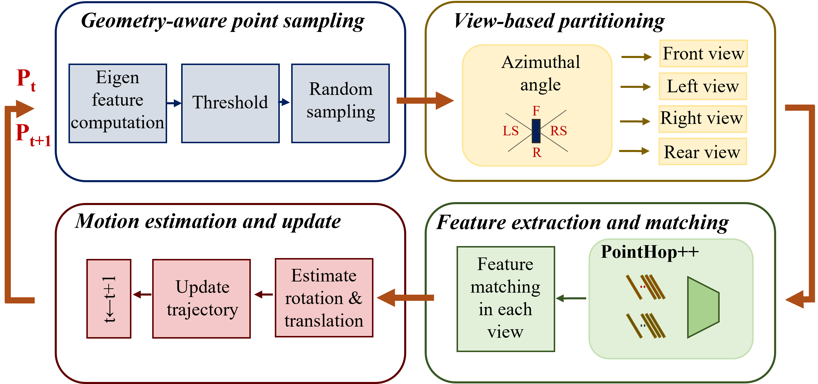
Figure 1: An overview of the GreenPCO method.

3.1 Geometry-aware point sampling

An outdoor point cloud scan captured by the LiDAR sensor typically consists of hundreds of thousands of points. However, many points in outdoor environments are featureless and non-discriminant. It is desirable and sufficient to select a subset of discriminant points to build a effective correspondence. To this end, we propose a geometry-aware point sampling method that selects points that are spatially spread out and with salient local characteristics.

The local neighborhood of a point, $p$, defines its local property. We collect $k$ nearest neighbors of $p$ in a local region, find the covariance matrix of their 3D coordinates, and conduct eigen decomposition. The eigenvalues of local PCA can describe the local characteristics of a point well. For examples, local features such as linearity, planarity, sphericity, and entropy can be expressed as functions of the three eigenvalues [27]. We are interested in discriminant points (e.g., those from objects like mopeds, cars, poles, etc.) rather than points from planar surfaces (e.g., buildings, roads, walls, etc.) To achieve this goal, we study distributions of eigenvalues and set appropriate thresholds so as to discard non-discriminant points in the pre-processing step. In our implementation, we set thresholds on linearity, planarity, and eigen entropy. They are computed as

$$\mbox{Linearity}=\frac{\lambda_{1}-\lambda_{2}}{\lambda_{1}} \hskip 14.22636pt\mbox{Planarity}=\frac{\lambda_{2}-\lambda_{3}}{\lambda_{1}},$$ ,

Eigen entropy $$= \sum_{i=1}^{3}\lambda_{i}\cdot\log(\frac{1}{\lambda_{i}}),$$ (2)

where $\lambda_{1}$, $\lambda_{2}$ and $\lambda_{3}$ are three eigenvalues of local PCA, and $\lambda_{1}\geq\lambda_{2}\geq\lambda_{3}$. After this step, we are left with around 4,000 to 5,000 points depending on the scene. Afterwards, we use random sampling to reduce the point number to 2,048 for further processing in the next step. Points selected by geometry-aware point sampling and random sampling are compared in Fig. 2. We see that the proposed geometry-aware sampling method preserves more discriminant points from the scene.

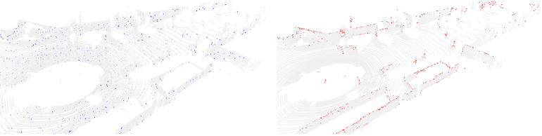
Figure 2: Comparison between random sampling (left) and geometry-aware sampling (right), where sampled points are marked in blue and red, respectively.

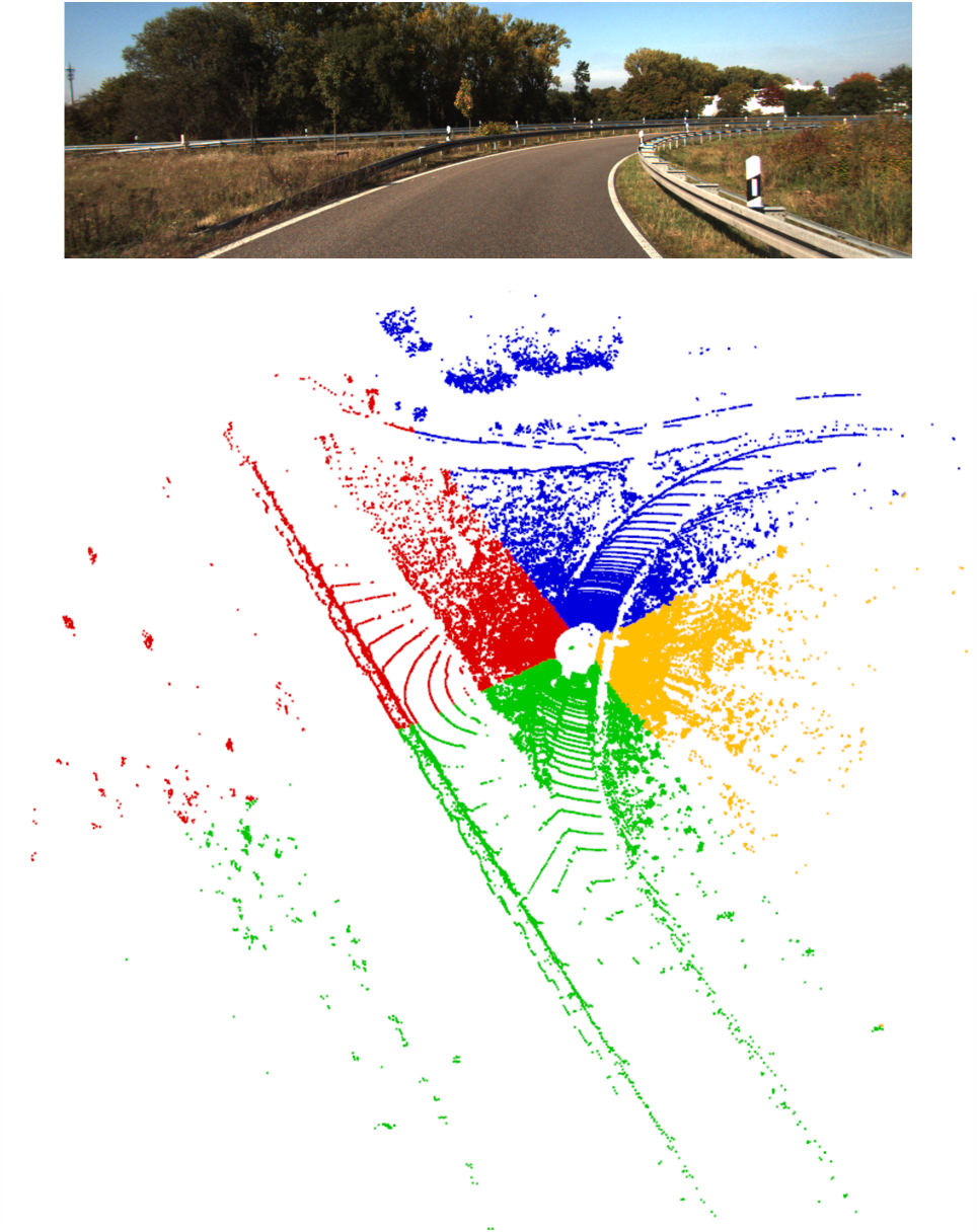
Figure 3: View-based partitioning using the azimuthal angle, where the front, rear, left and right views are highlighted in blue, green, red, and yellow, respectively.

3.2 View-based partitioning

The sampled points obtained in the previous step are divided into disjoint sets based on their 3D coordinates. First, the 3D Cartesian coordinates are converted to spherical coordinates. Following the convention of the LiDAR coordinate system setup in the KITTI dataset, the positive $Z$ direction is along the direction of motion of the vehicle, while the positive $Y$ direction is vertical. We are interested in the azimuthal angle $\phi$, which is given by

$$\phi=\arctan(z/x),$$ (3)

where $z$ and $x$ are point coordinates along the $Z$ and $X$ axes, respectively. The $\phi$ coordinate of every point gives the position of the point with respect to the vehicle. Then, we can define four views based on $\phi$. Front view contains points with an azimuthal angle $45^{\circ}\leq\phi\leq 135^{\circ}$. Rear view contains points with an azimuthal angle $225^{\circ}\leq\phi\leq 315^{\circ}$. Right side view contains points with an azimuthal angle $-45^{\circ}\leq\phi\leq 45^{\circ}$, and left side view contains points with an azimuthal angle $135^{\circ}\leq\phi\leq 225^{\circ}$. An example of view-based partitioning is shown in Fig. 3.

Since motion between two consecutive scans is incremental, we can focus on point matching in the same view. The proposed partitioning helps in scenarios when there are similar instances (e.g., persons or equally spaced poles along the road in different views) in two point cloud scans. We also tried to partition points into six disjoint views but observed no advantage. On the contrary, the probability of correctly matched points coming from different views increases. Thus, we stick to the choice of four views.

3.3 Feature extraction and point matching

The features of all points sampled in Step 1 are extracted using PointHop++ as described in [24]. Briefly speaking, the $k$ nearest neighbors of points are retrieved and the 3D coordinate space is partitioned into 8 octants. The mean of each octant is calculated and the eight means are concatenated to form the attribute vector. Then, the channel-wise Saab transform is conducted for dimension reduction. The attribute construction and dimensionality reduction step is repeated in the second hop to increase the receptive field. We append the 3D coordinates with the eigen features [27] to obtain a rich set of point features. For point matching in two point cloud scans, we consider the nearest neighbor search in the feature space and conduct it in each of the four view groups independently. As a result, we have four sets of point correspondences - one from each view. All corresponding pairs are then combined and used to estimate the rotation and translation between the two scans. A subset of matched points between two consecutive scans are shown in Fig. 4.

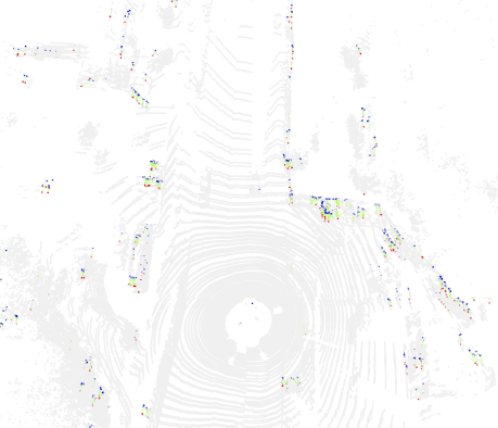
Figure 4: Sampled points at time instances $t$ and $t+1$ are marked in blue and red, respectively, while point correspondences between two consecutive scans are shown in green.

3.4 Motion estimation and update

The matched points found in Step 3 are used to estimate the motion between the two consecutive time instances. Suppose that $(x_{i},y_{i})$, $i=1,\cdots,N$, are the pairs of corresponding points. The 6-DOF motion model can be determined as follows. First, the mean coordinates of the corresponding points can be written as

$$\bar{x}=\frac{1}{N}\sum\limits_{i=1}^{N}x_{i},\quad\bar{y}=\frac{1}{N}\sum\limits_{i=1}^{N}y_{i},$$ (4)

and the covariance matrix of the corresponding pairs of points can be computed as

$$K(X,Y)=\sum\limits_{i=1}^{N}(x_{i}-\bar{x})(y_{i}-\bar{y})^{T}.$$ (5)

Next, the $3\times 3$ covariance matrix can be decomposed via SVD,

$$K(X,Y)=USV^{T},$$ (6)

where $U$ and $V$ are orthogonal matrices of left and right singular vectors and $S$ is the diagonal matrix of singular values, respectively. Then, the orientation and translation motion model are given by the rotation matrix, $R$, and the translation vector, $t$, in the form of

$$R=VU^{T},\mbox{ and }t=-R\bar{x}+\bar{y}.$$ (7)

The vehicle trajectory is updated with the current predicted pose. The pose at time $t$, $T^{t}$, with respect to the pose at time $t-1$, $T^{t-1}$, is given by $T^{t}=T^{t-1}[R\ t\ ;\ {\bar{0}}^{T}\ 1]$. The pose with respect to the the inital pose $T^{0}$ can be found accordingly. The process repeats by considering the next two point cloud scans. Furthermore, RANSAC [28] can be used to improve the robustness of point matching.

4 Experimental Results

Experiments are conducted on the KITTI Visual Odometry/SLAM benchmark [2] for performance evaluation. The dataset consists of 22 sequences in total, out of which the ground truth information is available for the first 11 sequences. Each sequence is a vehicle trajectory that consists of from 250 to 2000 time steps. The data at each time step contains the 3D point cloud scan captured by the LiDAR scanner, stereo and monocular images. By following point cloud odometry benchmarking methods such as DeepPCO [14], we use the point cloud data only in the experiments, we use sequences 4 and 10 for testing and the rest for training. It is observed that there is a strong correlation between scans of the training data. For this reason, we uniformly sample 50 point clouds from the nine training sequences to learn the kernels in channel-wise Saab transform. Furthermore, the geometry-aware sampling process is used to select discriminant points. The thresholds for the eigen features during sampling are set to 0.7 for linearity and planarity and 0.8 for eigen entropy. Points with their linearity and planarity below the 0.7 threshold and with their eigen entropy higher than the 0.8 threshold are retained. The neighborhood size for finding the eigen features is 48 points. Two hops are used in total.

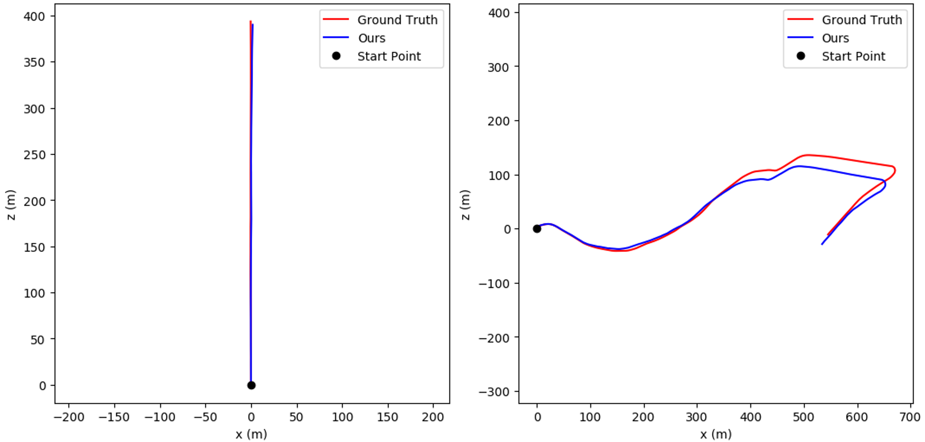
Figure 5: Results on sequences 4 (left) and 10 (right) of the KITTI dataset.

The evaluation results for test sequences 4 and 10 are shown in Fig. 5. We see that GreenPCO is very effective and its predicted paths almost overlap with the ground truth ones. Based on the KITTI evaluation metric, the average sequence translation RMSE is 3.54% while the average sequence rotation error is 0.0271 deg/m. We compare GreenPCO with five supervised DL methods in Table 1. They are Two-stream [13], DeepVO [16], PointNet [10], PointGrid [29] and DeepPCO [14]. The evaluation metrics are the same as those in DeepPCO [14], where relative translation and rotation errors are considered. Although GreenPCO is an unsupervised learning method, it outperforms all supervised DL methods in both the average rotation RMSE and the average translation RMSE.

Table 1: Performance comparison between GreenPCO and five supervised DL methods on two test sequences in the KITTI dataset

	Sequence 4		Sequence 10
Method	Avg. translation RMSE	Avg. rotation RMSE	Avg. translation RMSE	Avg. rotation RMSE
Two-stream [13]	0.0554	0.0830	0.0870	0.1592
DeepVO [16]	0.2157	0.0709	0.2153	0.3311
PointNet [10]	0.0946	0.0442	0.1381	0.1360
PointGrid [29]	0.0550	0.0690	0.0842	0.1523
DeepPCO [14]	0.0263	0.0305	0.0247	0.0659
GreenPCO (Ours)	0.0201	0.0212	0.0209	0.0628

We conduct an ablation study on GreenPCO to see the contributions of each component and summarize the results in Table 2. First, we compare geometry-aware, random, and farthest point sampling methods. For each sampling method, we set the number of sampled points to 1024, 2048, and 4096 points. Geometry-aware sampling consistently outperforms the other two. The errors of random sampling are worst while errors of farthest point sampling are also large. There is no advantage of using 4096 points over 2048 points for any sampling method. Thus, we set the input point number to 2048. Next, we justify the inclusion of view-based partitioning and eigen features. Errors are consistently lower when view-based partitioning is adopted. This shows that view-based partitioning makes point matching more robust. Furthermore, it reduces the search space for time efficiency. Finally, when eigen features are omitted from the feature construction process, the performance drops sharply.

Table 2: Ablation study on KITTI dataset

Sampling Method	Number of sampled points	View-based partitioning	Eigen features	Translation error (%)	Rotation error (deg/m)
Random	1024	✓	✓	32.42	0.1120
	2048	✓	✓	32.20	0.1179
	4096	✓	✓	31.47	0.1004
Farthest point	1024	✓	✓	28.79	0.1065
	2048	✓	✓	28.11	0.0971
	4096	✓	✓	28.13	0.0941
Geometry-aware	1024	✓	✓	3.71	0.0345
	2048	✓	✓	3.54	0.0271
	4096	✓	✓	3.54	0.0308
	2048			10.41	0.0415
	2048		✓	4.89	0.0289
	2048	✓		9.81	0.0401

Since most of the model-free methods such as LOAM [3] and V-LOAM [4] already offer state-of-the-art results, spending a large amount of time on model training (like deep learning) is not an optimal choice for this problem. GreenPCO is more favorable in this sense. Its training time is only 10 minutes on Intel Xeon CPU.

The rapid training time of GreenPCO is attributed to two reasons. First, PointHop++ model training demands sampled points to learn filter parameters. Other steps in the pipeline such as view-based partitioning, point matching, and motion estimation are only required during testing. Second, we use an extremely small training set since there is a high correlation between consecutive point cloud scans in different sequences due to incremental vehicular motion. Hence, skipping several scans and selecting only distant scenes should be sufficient to capture different scenes within the training data. It is observed that the use of 50 point cloud scans offers performance similar to that using the entire training dataset which comprises of 8500 scans. This corresponds to approximately 0.6% of the training data.

In our implementation, the 50 point cloud scans are uniformly sampled from the entire training dataset so as to represent diverse scenes. Table 3 summarizes the test performance for four different percents of training data. As shown in the table, the translation and rotation errors are unaffected and there is no advantage of using the entire training data. There is a steady decrease in the training time as the size of the training data is reduced. The model size is 75kB, which is independent of the training data used. A small model size and less training time make GreenPCO a lightweight solution for point cloud odometry.

Table 3: The effect of different amounts of training data

Training data used (%)	Training time (hours)	Model size	Translation error (%)	Rotation error (deg/m)
100	1.2	75kB	3.54	0.0268
50	0.8	75kB	3.53	0.0272
25	0.6	75kB	3.54	0.0271
10	0.5	75kB	3.54	0.0271
0.6	0.17	75kB	3.54	0.0271

5 Conclusion and Future Work

An unsupervised lightweight learning method for point cloud odometry, called GreenPCO, was proposed in this work. GreenPCO takes consecutive point cloud scans captured by the LiDAR sensor on the vehicle and estimates the 6-DOF motion of the vehicle incrementally. It first selects a small set of discriminant points using geometry-aware sampling. Then, the sampled points are divided into four disjoint sets based on the azimuthal angle. The point features are extracted using the PointHop++ method and matching points are found by searching neighbors in the feature space. Finally, the corresponding points are used to estimate the rotation and translation between the two positions. The same process is repeated for subsequent scans. GreenPCO gives accurate vehicle trajectories when evaluated on the LiDAR scans from the KITTI dataset. It outperforms all supervised DL-based benchmarking methods with much less training data.

As a future extension, it is worthwhile to analyze failure cases of the model-free methods based on scan matching and see whether replacing their handcrafted features with our learned features helps overcome their drawbacks. This opens a new research direction in exploiting traditional methods with unsupervised feature learning based on data statistics. Also, we applied GreenPCO to an outdoor PCO in this work. We expect that the same technique can be extended to indoor and/or other restricted environments with minor adjustments. The generalization to mobile robots or other moving agents should be valuable in real-world applications.

References

- [1] Pranav Kadam, Min Zhang, Shan Liu, and C-C Jay Kuo. R-PointHop: A Green, Accurate and Unsupervised Point Cloud Registration Method. arXiv preprint arXiv:2103.08129, 2021.
- [2] Andreas Geiger, Philip Lenz, and Raquel Urtasun. Are we ready for Autonomous Driving? The KITTI Vision Benchmark Suite. In Conference on Computer Vision and Pattern Recognition (CVPR), 2012.
- [3] Ji Zhang and Sanjiv Singh. LOAM: Lidar Odometry and Mapping in Real-time. In Robotics: Science and Systems, volume 2, 2014.
- [4] Ji Zhang and Sanjiv Singh. Visual-lidar odometry and mapping: Low-drift, robust, and fast. In 2015 IEEE International Conference on Robotics and Automation (ICRA), pages 2174–2181. IEEE, 2015.
- [5] Dávid Rozenberszki and András L Majdik. LOL: Lidar-only Odometry and Localization in 3D point cloud maps. In 2020 IEEE International Conference on Robotics and Automation (ICRA), pages 4379–4385. IEEE, 2020.
- [6] Raul Mur-Artal, Jose Maria Martinez Montiel, and Juan D Tardos. ORB-SLAM: a versatile and accurate monocular SLAM system. IEEE transactions on robotics, 31(5):1147–1163, 2015.
- [7] Igor Cvišić, Ivan Marković, and Ivan Petrović. Recalibrating the KITTI Dataset Camera Setup for Improved Odometry Accuracy. arXiv preprint arXiv:2109.03462, 2021.
- [8] Paul J Besl and Neil D McKay. Method for registration of 3-D shapes. In Sensor fusion IV: control paradigms and data structures, volume 1611, pages 586–606. International Society for Optics and Photonics, 1992.
- [9] Szymon Rusinkiewicz and Marc Levoy. Efficient variants of the ICP algorithm. In Proceedings third international conference on 3-D digital imaging and modeling, pages 145–152. IEEE, 2001.
- [10] Charles R Qi, Hao Su, Kaichun Mo, and Leonidas J Guibas. Pointnet: Deep learning on point sets for 3d classification and segmentation. In Proceedings of the IEEE conference on computer vision and pattern recognition, pages 652–660, 2017.
- [11] Charles R Qi, Li Yi, Hao Su, and Leonidas J Guibas. Pointnet++: Deep hierarchical feature learning on point sets in a metric space. arXiv preprint arXiv:1706.02413, 2017.
- [12] Yue Wang, Yongbin Sun, Ziwei Liu, Sanjay E Sarma, Michael M Bronstein, and Justin M Solomon. Dynamic graph cnn for learning on point clouds. Acm Transactions On Graphics (tog), 38(5):1–12, 2019.
- [13] Austin Nicolai, Ryan Skeele, Christopher Eriksen, and Geoffrey A Hollinger. Deep learning for laser based odometry estimation. In RSS workshop Limits and Potentials of Deep Learning in Robotics, volume 184, page 1, 2016.
- [14] Wei Wang, Muhamad Risqi U Saputra, Peijun Zhao, Pedro Gusmao, Bo Yang, Changhao Chen, Andrew Markham, and Niki Trigoni. Deeppco: End-to-end point cloud odometry through deep parallel neural network. In 2019 IEEE/RSJ International Conference on Intelligent Robots and Systems (IROS), pages 3248–3254. IEEE, 2019.
- [15] Kishore Reddy Konda and Roland Memisevic. Learning visual odometry with a convolutional network. In VISAPP (1), pages 486–490, 2015.
- [16] Sen Wang, Ronald Clark, Hongkai Wen, and Niki Trigoni. Deepvo: Towards end-to-end visual odometry with deep recurrent convolutional neural networks. In 2017 IEEE International Conference on Robotics and Automation (ICRA), pages 2043–2050. IEEE, 2017.
- [17] Ronald Clark, Sen Wang, Hongkai Wen, Andrew Markham, and Niki Trigoni. Vinet: Visual-inertial odometry as a sequence-to-sequence learning problem. In Proceedings of the AAAI Conference on Artificial Intelligence, volume 31, 2017.
- [18] Peter Muller and Andreas Savakis. Flowdometry: An optical flow and deep learning based approach to visual odometry. In 2017 IEEE Winter Conference on Applications of Computer Vision (WACV), pages 624–631. IEEE, 2017.
- [19] Gabriele Costante and Thomas Alessandro Ciarfuglia. LS-VO: Learning dense optical subspace for robust visual odometry estimation. IEEE Robotics and Automation Letters, 3(3):1735–1742, 2018.
- [20] Pranav Kadam, Min Zhang, Shan Liu, and C-C Jay Kuo. Unsupervised Point Cloud Registration via Salient Points Analysis (SPA). In 2020 IEEE International Conference on Visual Communications and Image Processing (VCIP), pages 5–8. IEEE, 2020.
- [21] Pranav Kadam, Qingyang Zhou, Shan Liu, and C-C Jay Kuo. Pcrp: Unsupervised point cloud object retrieval and pose estimation. arXiv preprint arXiv:2202.07843, 2022.
- [22] Min Zhang, Pranav Kadam, Shan Liu, and C-C Jay Kuo. Unsupervised feedforward feature (uff) learning for point cloud classification and segmentation. In 2020 IEEE International Conference on Visual Communications and Image Processing (VCIP), pages 144–147. IEEE, 2020.
- [23] Min Zhang, Pranav Kadam, Shan Liu, and C-C Jay Kuo. GSIP: Green Semantic Segmentation of Large-Scale Indoor Point Clouds. arXiv preprint arXiv:2109.11835, 2021.
- [24] Min Zhang, Yifan Wang, Pranav Kadam, Shan Liu, and C-C Jay Kuo. PointHop++: A lightweight learning model on point sets for 3D classification. In 2020 IEEE International Conference on Image Processing (ICIP), pages 3319–3323. IEEE, 2020.
- [25] Min Zhang, Haoxuan You, Pranav Kadam, Shan Liu, and C-C Jay Kuo. PointHop: An explainable machine learning method for point cloud classification. IEEE Transactions on Multimedia, 22(7):1744–1755, 2020.
- [26] C-C Jay Kuo, Min Zhang, Siyang Li, Jiali Duan, and Yueru Chen. Interpretable convolutional neural networks via feedforward design. Journal of Visual Communication and Image Representation, 60:346–359, 2019.
- [27] Timo Hackel, Jan D Wegner, and Konrad Schindler. Fast semantic segmentation of 3D point clouds with strongly varying density. ISPRS annals of the photogrammetry, remote sensing and spatial information sciences, 3:177–184, 2016.
- [28] Martin A Fischler and Robert C Bolles. Random sample consensus: a paradigm for model fitting with applications to image analysis and automated cartography. Communications of the ACM, 24(6):381–395, 1981.
- [29] Truc Le and Ye Duan. Pointgrid: A deep network for 3d shape understanding. In Proceedings of the IEEE conference on computer vision and pattern recognition, pages 9204–9214, 2018.