Random fixed points, systemic risk and resilience of heterogeneous financial network

Abstract

We consider a large random network, in which the performance of a node depends upon that of its neighbours and some external random influence factors. This results in random vector valued fixed-point (FP) equations in large dimensional spaces, and our aim is to study their almost-sure solutions. An underlying directed random graph defines the connections between various components of the FP equations. Existence of an edge between nodes $i,j$ implies the $i$-th FP equation depends on the $j$-th component. We consider a special case where any component of the FP equation depends upon an appropriate aggregate of that of the random ‘neighbour’ components. We obtain finite dimensional limit FP equations in a much smaller dimensional space, whose solutions aid to approximate the solution of FP equations for almost all realizations, as the number of nodes increases. We use Maximum theorem for non-compact sets to prove this convergence.

We apply the results to study systemic risk in an example financial network with large number of heterogeneous entities. We utilized the simplified limit system to analyse trends of default probability (probability that an entity fails to clear its liabilities) and expected surplus (expected-revenue after clearing liabilities) with varying degrees of interconnections between two diverse groups. We illustrated the accuracy of the approximation using exhaustive Monte-Carlo simulations.

Our approach can be utilized for a variety of financial networks (and others); the developed methodology provides approximate small-dimensional solutions to large-dimensional FP equations that represent the clearing vectors in case of financial networks.

1 Introduction

Random fixed points (FPs) are generalization of classical deterministic fixed points, and arise when one considers systems with uncertainty. One can think of two types of fixed points under uncertainty. There is considerable literature that considers stochastic fixed point equations on the space of probability distributions (e.g., Urns ; WeightedBranch ). These equations typically arise as a limit of some iterative schemes, or as asymptotic (stationary) distribution of stochastic systems. Alternatively, one might be interested in sample wise (almost sure) fixed points as in Measure_FP ; Measure_Approx ; for each realization of the random quantities describing the system, there is one deterministic fixed point equation. These kind of equations can arise when the performance/status of an agent depends upon that of other agents. For example, a financial network with any given liability graph is affected by individual/common random economic shocks received by the agents (see Section 5 for more details). The amount cleared (full/fraction of liability) by an agent depends upon: a) the random shocks it receives; and b) the liabilities cleared by the other agents. Our focus in this paper is on the second type of equations, defined in almost sure sense. Current literature primarily considers the existence of measurable fixed point solutions, given the existence of realization-wise fixed point solutions (e.g., Measure_FP ; Measure_Approx ). In Measure_Approx (and reference therein) authors consider the idea of random proximity points.

To the best of our knowledge, there are no (common) techniques that provide ‘good’ solutions to (even some special type of) these equations. We consider special type of fixed point equations, and provide a procedure to compute the approximate almost sure solutions; here the performance/status of an agent is influenced only by the aggregate performance/status of its neighbours.

We consider a random graph where nodes denote agents and the edges denote interaction between the agents. For example in a financial setting, nodes may be banks and edges may denote liability structure between banks. A set of fixed point equations (one per realization of the random quantities, e.g., economic shocks) describe certain performance vectors of the agents. The performance of each agent is influenced by aggregate of the performance of its neighbours, with the aggregate defined using the random edges. For example the clearing vectors in the financial setting.

The key idea is to study these fixed points, asymptotically as the number of agents increase. Towards this, we first analyze the aggregate influence factors, with an aim to reduce the dimensionality of the problem. But due to random connections, the aggregate influence factors can also depend upon the nodes. However the aggregates might converge towards the same limit almost surely (e.g., as in law of large numbers). Considering such scenarios, the random fixed points are shown to converge to that of a limit system, under certain conditions. The performance of the agents in the limit system, depends upon finitely many ‘aggregate’ limits. For some examples, closed-form expressions are derived for approximate almost sure solutions.

The mean-field theory primarily deals with a system of large number of agents, wherein the state/behaviour of an individual agent is influenced by its own (previous) state and the mean (aggregate) field seen by it (e.g., Mean_WLAN and reference therein). The mean-field is largely described in terms of occupation (empirical) measures representing the fraction of agents in different states. The theory shows the convergence of the mean state trajectories as well as the stationary (time limit) distributions of the original system towards that of a limit deterministic system.

The stationary distribution can be described by fixed point equations in the space of distributions (e.g., Mean_WLAN ). As opposed to that, we consider a set of fixed point equations, which are defined in almost sure sense.

We consider fixed point equations with possibly multiple solutions, and, show that any chosen sequence of the fixed points converge almost surely to a fixed point of the limit system (along a sub-sequence). Towards this, we construct an appropriate parameterized optimization problem and apply the relatively recent result (Feinberg ) on Maximum Theorem for non-compact sets to show almost sure convergence of the aggregate random fixed points; the main idea is to construct appropriate topological spaces (e.g., Tychonoff’s topology) and an appropriate objective function. Under some additional (mild) conditions, we show the uniqueness of the fixed points; we further derive limit solutions using that of a significantly low-dimensional system. The results are derived for the case with two diverse groups (homogeneous within the group) of agents, for which one has to solve three-dimensional equations; one can easily extend the results to any finite number of groups.

Application to financial networks

We apply our results to study systemic risk related aspects in a large financial network. The institutions borrow/lend money from/to other institutions, and will have to clear their obligations at a later time. These systems are subjected to economic shocks, because of which some entities default (do not clear their obligations). Because of inter-dependencies, this can lead to further defaults and the cascade of these reactions can lead to the (partial/full) collapse of the system.

After the financial crisis of $2007$-$2008$, there is a surge of activity towards studying systemic risk (e.g.,acemoglu2015systemic ; allen2000financial ; eisenberg2001systemic ). The focus in these papers has been on several aspects including, measures to capture systemic risk, influence of network structure on systemic risk, phase transitions etc. Some papers (e.g., allen2000financial ; blume2011networks ; eisenberg2001systemic ; Systemicrisk ; Freixas ; Haldane ) consider network-based approach, while carmona2013mean ; Garnier considers mean-field analysis based approach. Further these papers primarily discuss homogeneous systems, although heterogeneity is a crucial feature of real world networks. As already mentioned, the clearing vectors are represented by FP equations and one must analyze the same to study the more realistic heterogeneous networks; our asymptotic solution can be of significant relevance in this context.

The seminal work in this line of research is provided by allen2000financial , which shows that incomplete financial networks are less resilient and more vulnerable to contagion than complete networks (all nodes are interconnected as in complete graph). A similar kind of conclusions are derived in Freixas , in the context of liquidity shocks. Another piece of pioneering work is eisenberg2001systemic , wherein, the authors show that the clearing payment vector is unique under mild conditions. The paper also provides a fictitious default algorithm to compute the clearing vector. In recent years, the authors of acemoglu2015systemic extended the work of eisenberg2001systemic , to accommodate the external shocks; they also showed the stability of complete graph (when the magnitude of the negative shock is below a specific range) and vulnerability of the ring graphs among all regular class of networks.

The previous papers consider time-static models, while acemoglu2015systemic also considers three time-period model; at time $t=0$ the portfolio is chosen, partial returns and liability repayment is at $t=1$ and the final returns (in case of no default) are at $t=2$.

Majority of the papers discussed above consider deterministic networks. Real world networks are seldom deterministic, it is more appropriate to model them using random quantities. Authors in Glasserman consider random networks and derive a network independent bound on the probability of financial contagion. The authors in Amini also consider random networks, and derive analysis under the assumption that the recovery rate is negligible for the defaulted nodes.

Our results related to financial networks

We consider random networks with diverse groups (homogeneous agents within each group), two-time period return model and with random economic shocks. Further the defaulted banks pay-back their liabilities to the best extent possible. Under certain growth condition on the number of neighbours (in each group) we derived a very general technique to obtain approximate closed form expressions (easily computable) for clearing vectors. Our methods can handle a large variety of networks and the approximate clearing vectors can be used in computing a variety of performance measures, e.g., default probability, expected surplus. For example, in this paper we consider a network with two sets of users, the first group takes measured risk and the second group is aggressive while choosing their portfolios at time $t=0$. We identified a regime of parameters (interest rates, parameters of economic shocks, percentage of taxes etc.) in which both the groups benefit by small amount of inter-connections between the two groups; for the rest of the regimes, only one of the groups benefits.

One can use our clearing vector based results to study various other aspects. In Saha we used these results to study the convergence of replicator dynamics in a financial network where the agents alter their choices between risk-free or risky portfolios (based on their experiences and observations). We showed that all the agents eventually revert either to risky or risk-free portfolios, unless the agents choose their strategies based on large number of observations. In the former case the dynamics converges to pure evolutionary stable strategy (ESS), while the latter converges to a mixed ESS.

Some initial results of this flavour are available in our conference paper Systemicrisk . However, the current paper is a sufficient generalization; we consider a more complex network/graph with a larger variety of entities to define the FP equations and also prove the results using alternate assumptions on graph structure. In addition, the current paper includes all the relevant proofs. We also analyze a more complex financial network. Further using exhaustive Monte-Carlo simulations, we illustrate good accuracy of approximation even for moderate-sized networks. To summarise, our analysis helps identify important patterns in a complex structure, since the structure (often) simplifies when large number of constituents are involved.

Organization of the paper: The rest of the paper is organized as follows: Sections 2 and 3 provide random fixed point almost sure results for two different structures of the network. Section 4 provides various other graphical models. Section 5 describes the large financial system, while, Section 6 provides its asymptotic analysis. We have Monte-Carlo simulations in Section 7 and Section 8 concludes the paper. All the proofs are provided in the Appendices.

2 Graphical model and fixed point equations

We consider $(n+1)$ nodes in a random network indexed by the set $N$ whose directed edges, have random weights $\{W_{j,i}\}$, representing influence factors. The node $b\in N$ is a big node and has significant influence on the network. The remaining $n$ nodes are small nodes and are classified into two groups $\mathcal{G}_{1}$ and $\mathcal{G}_{2}$ respectively. The size of the group $\mathcal{G}_{1}$ is $n_{1}=n\gamma$ and that of $\mathcal{G}_{2}$ group is $n_{2}=n(1-\gamma)$, where $0<\gamma<1$ is a positive fraction. Let ${\cal G}_{1}=\{1,2,\cdots,n_{1}\}\mbox{ and }{\cal G}_{2}=\{1,\cdots,n_{2}\}.$ Any small node in $N$ is represented by pair $(m,i)$ with $i\leq n_{m}$ and $m\in\{1,2\}$.

The probability of an edge connecting two small nodes belonging to the same group (say $\mathcal{G}_{m}$) is $p_{m}$, while, that of an edge connecting two nodes belonging to different groups is $p_{c_{1}}$ or $p_{c_{2}}$. All the edge forming events are independent of the others (or need to satisfy B.2(C) defined later, if some connections are correlated) and let $\{I_{j,i}\}$, be the corresponding indicators. To summarize, for any $i\in{\cal G}_{m}$ and $j\in{\cal G}_{m^{\prime}}$:

$$P(I_{j,i}=1)=p_{mm^{{}^{\prime}}}=\left\{\begin{array}[]{llll}p_{m}&\mbox{ if }m=m^{{}^{\prime}}\mbox{, }\mbox{ for any }m\in\{1,2\}\mbox{ and }\\ p_{c_{1}}&\mbox{ if }~{}~{}j\in\mathcal{G}_{1}~{}~{}and~{}~{}i\in\mathcal{G}_{2},\\ p_{c_{2}}&\mbox{ if }~{}~{}j\in\mathcal{G}_{2}~{}~{}and~{}~{}i\in\mathcal{G}_{1}.\end{array}\right.$$ (4)

From any small node $j\in\mathcal{G}_{m}$, there is a dedicated fraction $\eta^{sb}_{j}$ (of weight) towards the b-node while the remaining ($1-\eta^{sb}_{j}$) fraction is shared by other connected small nodes. This fraction, for example, can represent an investment to a particular stock of a big player or to a government security or to a nationalized bank (more details are in Section 5, that discusses finance based application). In all, weights from a small node $j\in\mathcal{G}_{m}$ are the respective fractions as below:

$$W_{j,b} = \eta_{j}^{sb}\mbox{ (to b-node),}\ \ W_{j,i}=\frac{I_{j,i}(1-\eta_{j}^{sb})}{\displaystyle\sum_{i^{\prime}\in\mathcal{G}_{1}\cup\mathcal{G}_{2}}I_{j,i^{\prime}}},\mbox{ (to another small node $i$)},\mbox{ with}$$

$$p_{m}^{sb} := E[\eta_{j}^{sb}]\mbox{ for any }j\in{\cal G}_{m}.$$ (5)

In the above, $\{\eta_{j}^{sb}\}_{j\in{\cal G}_{m}}$, are i.i.d. (independent and identically distributed) random variables with values between $0$ and $1$ for any $m$ and are independent of all other random variables. The weights from $b$-node are given by $\{\eta_{j}^{bs}\}$, where $\{\eta_{j}^{bs}\}_{j\in{\cal G}_{m}}$, are bounded i.i.d. random variables for any $m$ and are independent of others. We consider an alternate form of interconnections in Section 3.

We are interested in the performance of the nodes, which depends upon the weighted aggregate of the performance of other nodes with weights as given by $\{W_{j,i}\}_{j,i\in N}$, $\{\eta^{bs}_{j}\}$ and  $\{W_{j,b}\}$. As mentioned, the weights of the performance measures may be stochastically different for the two groups. We consider the following fixed-point (FP) equation (in $\mathcal{R}^{n+1}$) constructed using functions $(f^{1},f^{2},f^{b})$, which in turn depend upon weighted averages $\{{\bar{X}}^{m}_{i}\}_{i}$ and ${\bar{X}}^{b}$ (constructed using weights $\{W_{j,i}\}$ and $\{W_{j,b}\}$), and whose solution ($i$-th component) represents important performance measure of the nodes (node-$i$), as below:

$$X_{i}^{m} = f^{m}(G^{m}_{i},{\bar{X}}^{m}_{i},\eta_{i}^{bs}X^{b})\mbox{ {\normalsize for each }}i\in\mathcal{G}_{m},\ \mbox{and},$$ (6)

$$X^{b} = f^{b}({\bar{X}}^{b})\ \ \ \mbox{ {\normalsize with aggregates}}$$ (7)

$${\bar{X}}^{m}_{i} := \displaystyle\sum_{j\in\mathcal{G}_{1}}X_{j}^{1}W_{j,i}+\displaystyle\sum_{j\in\mathcal{G}_{2}}X_{j}^{2}{W}_{j,i}\mbox{ {\normalsize for each }}i\in\mathcal{G}_{m},\ \$$ (8)

$${\bar{X}}^{b} := \frac{1}{n}\sum_{j\in\mathcal{G}_{1}}{X}^{1}_{j}W_{j,b}+\frac{1}{n}\sum_{j\in\mathcal{G}_{2}}{X}^{2}_{j}W_{j,b}.$$ (9)

In the above, $\{G^{m}_{i}\}_{i}$ is an i.i.d. sequence for any fixed $m$ and further is independent of the sequence corresponding to other $m$ and other random variables; the performance of the big node $X^{b}$ is defined per small node (performance divided by $n$) and influences that of the small nodes via terms $\{\eta_{i}^{bs}X^{b}\}$. For any $n=n_{1}+n_{2}$ define mapping

$${\bf f}:=(f^{b},\underbrace{f^{1},f^{1},\cdots,f^{1}}_{n_{1}\mbox{ times }},\underbrace{f^{2},f^{2}\cdots f^{2}}_{n_{2}\mbox{ times }}),\mbox{ with }{\bf x}:=(x_{1}^{1},x_{2}^{1},\cdots x_{n_{1}}^{1},x_{1}^{2},\cdots x_{n_{2}}^{2}),$$ (10)

component wise as below ($m\in\{1,2\}$):

$$f_{1}(x_{b},{\bf x}) := f^{b}({\bar{x}}_{b}),\mbox{ with, }{\bar{x}}_{b}:=\frac{1}{n}\displaystyle\sum_{j\in\mathcal{G}_{1}}{x}^{1}_{j}W_{j,b}+\frac{1}{n}\sum_{j\in\mathcal{G}_{2}}{x}^{2}_{j}{W}_{j,b}\mbox{ and,}$$ (11)

$$f^{m}_{i}(x_{b},{\bf x}) := f^{m}(G_{i}^{m},{\bar{x}}_{i}^{m},\eta_{i}^{bs}x_{b}),\ \ {\bar{x}}^{m}_{i}:=\displaystyle\sum_{j\in\mathcal{G}_{1}}x^{1}_{j}W_{j,i}+\displaystyle\sum_{j\in\mathcal{G}_{2}}x^{2}_{j}{W}_{j,i}\ \forall i\in{\mathcal{G}_{m}}.\hskip 14.22636pt$$ (12)

It is clear that the above mapping represents the fixed point equations corresponding to the random operator (6)-(9), sample path wise (i.e., for each realization of the random variables, $\{G_{j}^{m}\}_{j,m},\{\eta_{j}^{bs}\}_{j},\{\eta_{j}^{sb}\}_{j},\{I_{j,i}\}_{j,i}$).

We assume the following:
B.1 The functions $f^{1}(.),f^{2}(.),f^{b}(.)$ are non-negative, continuous and are bounded by a constant $y<\infty$,

$$0\leq f^{1}(g_{1},x,x_{b}),f^{2}(g_{2},x,x_{b}),f^{b}(x_{b})\leq y\mbox{ for all }g_{1},g_{2},x,x_{b}.$$

This is a typical assumption required for existence of fixed points; we also require that the functions are bounded. This is a reasonable assumption as many applications satisfy this, including our financial network.

Under the above assumption, we have a measurable fixed point solution:

Lemma 1

For any $n$ consider mapping ${\bf f}$ defined as in (10)-(12). Then we have (almost sure) random fixed point $(X_{b}^{*},{\bf X}^{*})$ for each $n$ (see Measure_FP ).

Proof: Each component of this function is a mapping from $[0,y]^{n+1}\to[0,y]$ for almost all $\{G^{m}_{i}\}$, $\{W_{j,i}\}$. Thus the function ${\bf f}$ from $[0,y]^{n+1}\to[0,y]^{n+1}$. Further by continuity of ${\bf f}$, using the well known Brouwer’s fixed point Theorem, we have a deterministic fixed point for all realizations of $\{G^{m}_{i}\}$ , $\{W_{j,i}\}$, $\{W_{j,b}\}$ and $\{\eta_{j}^{bs}\}_{j}$ under B.1. Then the overall measurability result follows by (Measure_FP, , Theorem 8). . $\blacksquare$

Assumptions on the graph structure: We require that the number of nodes influencing any given node, grows asymptotically linearly with $n$ for almost all sample paths. Towards this, first define the following set:

$${\cal E} := \left\{\omega:\lim_{n\to\infty}\displaystyle\sum_{j\in\mathcal{G}_{1}}\left|\frac{1}{\displaystyle\sum_{i\in\mathcal{G}_{1}\cup\mathcal{G}_{2}}I_{j,i}}-\frac{1}{n\gamma_{{}_{p_{1}}}}\right|=0,~{}\lim_{n\to\infty}\displaystyle\sum_{j\in\mathcal{G}_{2}}\left|\frac{1}{\displaystyle\sum_{i\in\mathcal{G}_{1}\cup\mathcal{G}_{2}}I_{j,i}}-\frac{1}{n\gamma_{{}_{p_{2}}}}\right|=0\right\},$$ (13)

$$\mbox{\normalsize with, }\gamma_{{}_{p_{1}}}:=\gamma p_{1}+(1-\gamma)p_{c_{1}}\mbox{\normalsize and }\gamma_{{}_{p_{2}}}:=\gamma p_{c_{2}}+(1-\gamma)p_{2}.\hskip 5.69054pt$$

We require the following assumption, which has two parts. In part (C) we consider that $\{I_{j,i}\}$ need not be independent; however they remain independent of the other quantities like $\{G_{j}^{m}\}$, $\{\eta_{j}^{sb}\}_{j\in{\cal G}_{m}}$ etc:
B.2 Assume $\gamma_{{}_{p_{1}}}>0$ and $\gamma_{{}_{p_{2}}}>0$. Also consider only graphs for which, $P({\cal E})=1$.
B.2(C), extra assumption for correlated $\{I_{j,i}\}$: When $\{I_{j,i}\}_{j}$ are not i.i.d. we additionally require:

$$\frac{1}{n\gamma_{m}}\sum_{j\in{\cal G}_{m}}I_{j,i}\to p_{m^{\prime},m}\mbox{ a.s. }\mbox{ for any }m,m^{\prime}\mbox{ and }i\in\mathcal{G}_{m^{\prime}}.$$

The initial results are with this assumption, latter (in sub-section 2.2) we have results under more general conditions (with $P({\cal E})<1$). We also provide an equivalent assumption on the growth pattern of the graphs in the same sub-section.

Our assumptions on graph structure are quite general. We firstly require that the marginal probabilities related to random connections, are the same within a group, i.e., $P(I_{j,i}=1)=p_{mm^{\prime}}$ as in equation (4) (for each $i,j$). Further the joint probabilities are supposed to satisfy B.2, i.e., mainly $P({\cal E})=1$. Furthermore, when the connections $\{I_{j,i}\}$ are not independent, the results are still true under the most natural assumption B.2(C). Regular graphs constructed in sub-section 7 are some example graphs that satisfy our assumptions. Our results can also be extended partially to Erdős-Rényi graphs, if required via Theorem 3. The most restrictive assumption is B.2 and one can avoid such an assumption by considering a different structure on weights as discussed in sub-section 4 (see e.g., equation (4.1)). With this our results can cover many more graphs.

2.1 Aggregate fixed points:

We rewrite the fixed point equations in terms of weighted averages and first analyze the aggregate system. Towards this, define the following random variables, that depend upon real constants $({\bar{x}}^{m}_{i},x_{b})$:

$$\xi^{m}_{i}({\bar{x}}^{m}_{i},x_{b}):=f^{m}(G_{i}^{m},{\bar{x}}_{i}^{m},\eta_{i}^{bs}x_{b})\mbox{ for any }i\in{\cal G}_{m},$$ (14)

and assume for each value of $m\in\{1,2\}$ (see (4), (2)):

B.3 $|\xi^{m}_{i}(x,x_{b})-\xi^{m}_{i}(u,u_{b})|\leq\sigma(|x-u|+\varsigma|x_{b}-u_{b}|)$ with $\sigma\leq 1$ and $0<\varsigma\leq 1$. Basically we require the following:

$$|f^{b}({\bar{x}}_{b})-f^{b}({\bar{u}}_{b})| \leq |{\bar{x}}_{b}-{\bar{u}}_{b}|\mbox{ for all }{\bar{x}}_{b},{\bar{u}}_{b},\mbox{ and, }$$

$$|f^{m}(g,x,\eta x_{b})-f^{m}(g,u,\eta u_{b})| \leq \sigma(|x-u|+\varsigma|x_{b}-u_{b}|)\mbox{ for all }x,u,x_{b},u_{b},g,\eta.$$

B.3 is a typical contraction mapping type of assumption that ensures the existence (and uniqueness) of fixed points. Observe this assumption does not imply strict contraction mapping (as $\sigma\leq 1$ and not $\sigma<1$), but is nonetheless sufficient.
B.4 Assume $\varrho\leq 1$, where

$$\hskip 11.38109pt\varrho := \max\bigg{\{}\frac{\gamma p_{c_{1}}(1-p_{1}^{sb})}{\gamma_{{}_{p_{1}}}}+\frac{(1-\gamma)p_{2}(1-p_{2}^{sb})}{\gamma_{{}_{p_{2}}}},\ \ \ \ \ \frac{\gamma p_{1}(1-p_{1}^{sb})}{\gamma_{{}_{p_{1}}}}+\frac{(1-\gamma)p_{c_{2}}(1-p_{2}^{sb})}{\gamma_{{}_{p_{2}}}}\bigg{\}}$$

$$+\left(\gamma p_{1}^{sb}+(1-\gamma)p_{2}^{sb}\right).$$

Observe that B.4 is readily satisfied, for symmetric conditions, for example, when $\gamma=0.5$, $p_{1}^{sb}=p_{2}^{sb}$, $p_{1}=p_{2}$ and $p_{c_{1}}=p_{c_{2}}$.

Let ${\bar{\bf x}}^{m}:=({\bar{x}}^{m}_{1},{\bar{x}}^{m}_{2}\cdots)\mbox{ for }m\in\{1,2\}\mbox{ and }{{\bar{\bf x}}}:=({\bar{\bf x}}^{1},{\bar{\bf x}}^{2})$. Consider the following operators on Banach space $[0,y]\times s^{\infty}\times s^{\infty}$, one for each $n=n_{1}+n_{2}$:

$${\bar{\bf f}}^{n}({\bar{x}}_{b},{{\bar{\bf x}}}) = ({\bar{f}}^{n}_{b},\ \ \ {\bar{f}}_{1}^{n,1},{\bar{f}}_{2}^{n,1},\cdots,{\bar{f}}_{n_{1}}^{n,1},\cdots,\ \ \ {\bar{f}}_{1}^{n,2},\cdots,{\bar{f}}_{n_{2}}^{n,2},\cdots),$$ (15)

where for any $(n,m)$ we have,

$${\bar{f}}^{n,m}_{i}({\bar{x}}_{b},{\bar{\bf x}}) := \left\{\begin{array}[]{lll}\displaystyle\sum_{j\in\mathcal{G}_{1}}\xi^{1}_{j}({\bar{x}}^{1}_{j},x_{b})W_{j,i}+\displaystyle\sum_{j\in\mathcal{G}_{2}}\xi_{j}^{2}({\bar{x}}^{2}_{j},x_{b}){W}_{j,i}&\mbox{ if }i\in\mathcal{G}_{m},\\ 0&\mbox{\normalsize else,}\mbox{ \normalsize and, }\\ \end{array}\right.$$ (18)

$${\bar{f}}^{n}_{b}({\bar{x}}_{b},{{\bar{\bf x}}}) := \frac{1}{n}\displaystyle\sum_{j\in\mathcal{G}_{1}}\xi^{1}_{j}({\bar{x}}^{1}_{j},x_{b})W_{j,b}+\frac{1}{n}\displaystyle\sum_{j\in\mathcal{G}_{2}}\xi^{2}_{j}({\bar{x}}^{2}_{j},x_{b})W_{j,b}\ \mbox{\normalsize with }\ x_{b}:=f^{b}({\bar{x}}_{b}).$$

Thus we require the fixed point of the operator:

$${\bar{\bf f}}^{n}\mbox{ where }{\bar{\bf f}}^{n}:{[0,y]}\times{s}^{\infty}\times{s}^{\infty}\to{[0,y]}\times{s}^{\infty}\times{s}^{\infty},$$

which provides the aggregate vectors, $({\bar{X}}_{b},\{{\bar{X}}_{i}^{m}\}_{i\leq n_{m}})$ given in (8)-(9). Observe here that, for uniformity we have infinite dimensional mappings even for finite $n$, where the extra components are set to zero functions (i.e., ${\bar{f}}^{n,m}_{i}\equiv 0$ for all $i>n_{m}$).

Recall that the weights sum up to one, i.e., $\sum_{i}W_{j,i}+W_{j,b}=1$ for all $j$. Thus the idea is to derive a kind of mean-field analysis where their expected values will approximate the aggregates. Towards this, as a first step, we analyze the point-wise limits of the above operator.

Lemma 2

[Constant sequences] Assume B.1-B.2. Consider any constant sequence ${{\bar{\bf x}}}=({\bar{\bf x}}^{1},{\bar{\bf x}}^{2})$, i.e., sequence with ${\bar{\bf x}}^{m}=({\bar{x}}^{m},{\bar{x}}^{m},\cdots)$ for some ${\bar{x}}^{m}<\infty$, for each $m$. The functions ${\bar{\bf f}}^{n}({\bar{x}}_{b},{{\bar{\bf x}}})$ defined in (15)-(18) converge component-wise and the limits equal almost surely (with $x_{b}=f^{b}({\bar{x}}_{b})$ as in (7), and see (4)):

$${\bar{f}}_{i}^{\infty,m}({\bar{x}}_{b},{\bar{\bf x}}) = E_{G^{1}_{i},\eta_{i}^{bs}}\left[\xi^{1}_{i}({\bar{x}}^{1},x_{b})\right]\frac{\gamma p_{1m}}{\gamma_{{}_{p_{1}}}}(1-p_{1}^{sb})$$

$$+E_{G^{2}_{i},\eta_{i}^{bs}}\left[\xi^{2}_{i}({\bar{x}}^{2},x_{b})\right]\frac{(1-\gamma)p_{2m}}{\gamma_{{}_{p_{2}}}}(1-p_{2}^{sb})\ \mbox{for}\ i\in\mathcal{G}_{m},\ \forall m,$$

$${\bar{f}}_{b}^{\infty}({\bar{x}}_{b},{\bar{\bf x}}) = \gamma E_{G^{1}_{i},\eta_{i}^{bs}}[\xi^{1}_{i}({\bar{x}}^{1},x_{b})]p_{1}^{sb}+(1-\gamma)E_{{G}^{2}_{i},\eta_{i}^{bs}}[\xi^{2}_{i}({\bar{x}}^{2},x_{b})]p_{2}^{sb}.$$ (19)

Proof: is available in Appendix A. $\blacksquare$
In the above, $E_{X,Y}$ represents the expectation with respect to $X,Y$. For constant sequences the random variables $\{\xi^{m}_{i}(\bar{x}^{m},x_{b})\}_{i\in{\cal G}_{m}}$ are i.i.d., and hence the first equation of (19) has same right hand side value for all $i\in\mathcal{G}_{m}$. We now define the following ‘limit’ operator, which in view of the above lemma equals a limit for constant sequences:

$$\bar{\bf f}^{\infty}({\bar{x}}_{b},{\bar{\bf x}}) = ({\bar{f}}^{\infty}_{b},\ \ \ {\bar{f}}^{\infty,1}_{1},\cdots,\ \ \ {\bar{f}}^{\infty,2}_{1},\cdots)\mbox{ with}$$ (20)

$${\bar{f}}_{b}^{\infty}({\bar{x}}_{b},{\bar{\bf x}}) := \displaystyle\lim\sup_{n}{\bar{f}}^{n}_{b}({\bar{x}}_{b},{\bar{\bf x}})\ \mbox{and},$$

$${\bar{f}}_{i}^{\infty,m}({\bar{x}}_{b},{\bar{\bf x}}) := \displaystyle\lim\sup_{n}{\bar{f}}^{n,m}_{i}({\bar{x}}_{b},{\bar{\bf x}})\mbox{ for all }i\mbox{ and }m.$$

The idea is to show that the aggregate fixed points of the original system converge towards the fixed point of this ‘limit’ system/operator (20) (more specifically the fixed point of the three dimensional system (19)), as $n\to\infty$. We require another assumption:

B.5 The limit system ${\bar{f}}^{\infty}$ given by (20) has a fixed point among constant sequences.

The assumption B.5 demands that the limit system has a fixed point among constant sequences. This kind of an assumption can be restrictive, but provides required convergence results in the most general settings. Further it might be readily satisfied by some future applications; thus this assumption gives more flexibility for future applications. Furthermore, we prove this assumption (along with others) in Theorem 2 and the assumptions of the latter theorem are readily satisfied by the financial network based case studies of Section 5.

We now prove one of the the main results of this paper:

Theorem 1

Assume B.1-B.5. The aggregates of the random system (6)-(9), which are FPs of (14)-(15), denoted by $({\bar{X}}_{b},{{\bar{\bf X}}})(n)=({\bar{X}}_{b},\{{\bar{X}}_{i}^{m}\}_{i,m})(n)$, converge as $n\to\infty$ along a sub-sequence. That is, there exists $k_{n}\to\infty$ such that:

$${\bar{X}}_{i}^{m}(k_{n})\to{\bar{x}}_{i}^{m\infty*}\ \forall i,m,\mbox{ and }{\bar{X}}_{b}(k_{n})\to{\bar{x}}_{b}^{\infty*}\mbox{ almost surely (a.s.),}$$ (21)

where $({\bar{x}}_{b}^{\infty*},{\bar{\bf x}}^{\infty*})$ with ${\bar{\bf x}}^{\infty*}:=({\bar{x}}_{1}^{1\infty*},{\bar{x}}_{2}^{1\infty*},\cdots{\bar{x}}_{1}^{2\infty*},{\bar{x}}_{2}^{2\infty*},\cdots)$ is an FP of the limit system given by (20). Further (any sequence of) FPs of the original system (6)-(7) converge almost surely (along the sub-sequence of (21), i.e., as $k_{n}\to\infty$):

$$X^{b}(k_{n}) \to f^{b}({\bar{x}}_{b}^{\infty*})\mbox{ and }\hskip 8.53581pt\ X^{m}_{i}(k_{n})\ \to\ f^{m}(G_{i}^{m},{\bar{x}}_{i}^{m\infty*},\eta_{i}^{bs}X_{b}^{\infty*})\ \forall i,m.$$ (22)

Proof: available in Appendix B. $\blacksquare$
By the above theorem, under minimal conditions on the fixed points of the limit system (20), the fixed points of the finite $n$-system can be studied using that of the limit system, the latter is an approximation and the approximation would be better for larger $n$. We now consider an additional assumption under which one will have unique fixed points, and in addition, the FP is a constant sequence for limit system:

Theorem 2

[Unique fixed points] Assume B.1-B.4 and also assume $\eta_{j}^{sb}\geq\underline{\eta}\geq 0$ a.s., with $\sigma\left(1-\underline{\eta}+\varsigma\underline{\eta}\right)<1$. Then we have unique fixed point of the finite $n$-system (18) for each $n$. We also have unique fixed point for the limit system (20), which is a constant sequence, i.e., we have ${\bar{x}}_{i}^{m\infty*}={\bar{x}}^{m\infty*}$ for all $i\in{\cal G}_{m}$ and for each $m$ in equation (21). This limit is the unique fixed point of the three dimensional system given by (19).

Proof: available in Appendix B. $\blacksquare$
The above theorem immediately implies the following corollary: one can solve three dimensional system (19) and derive the fixed points for large dimensional system given by (6)-(7) almost surely.

Corollary 1

[Three dimensional approximation] Assume the conditions of Theorem 2. Then convergence in the equations (21)-(22) is along the original sequence, i.e., as $n\to\infty$. Further, $({\bar{x}}_{b}^{\infty*},{\bar{\bf x}}^{\infty*})$ is a constant sequence and is the unique fixed point of the three dimensional system given by (19).

Proof: available in Appendix B. $\blacksquare$
Remarks: We have several remarks regarding the above results.
$\bullet$ Observe that the aggregate fixed points converge almost surely to the same limit; further the aggregates at limit are also constant across the agents of the same group as given by Theorem 2 and Corollary 1.
$\bullet$ The fixed points of the finite $n$ system converge to that of the limit system. From (22) and Corollary 1, the fixed points are asymptotically independent and depend upon the other nodes only via an almost sure constant (representing the aggregate), which is the same for all $i$ in a group.

$\bullet$ Under the more general assumptions of the Theorem 1 the aggregate fixed points need not be unique, for initial $n$. However, any sequence of fixed points (one for each $n$) converges towards that of the limit system (when it has a unique fixed point). If the limit system has many fixed points then every such sub-sequence converge to one among these fixed points. Thus the three dimensional fixed points of (19) (if any) are useful even under general conditions.

$\bullet$ The graphical model of the current paper is a significantly generalised version of our previous model considered in Systemicrisk ; and it reduces to the model considered in Systemicrisk , when $p_{1}=p_{2}=p_{c_{1}}=p_{c_{2}}=p_{ss}$ and $\gamma\in\{0,1\}$. Also, the current graphical model is heterogeneous in many more aspects, e.g., the interconnection probabilities, the connections to b-node etc.
$\bullet$ From (19), the limiting fixed point is dependent on the interconnection probability ($p_{c_{m}}$) as well as the group-wise connectivity parameters ($\{p_{m}\}$). While in our initial model of Systemicrisk , with only one group and a big node, the limiting fixed point is independent of the exact value of the connectivity parameter (referred to as $p_{ss}$ in Systemicrisk ); it only requires that $p_{ss}>0$ (together with other appropriate assumptions on graph structure). Thus it establishes that when more groups are coupled, the limits depend upon inter-group as well as intra-group connectivity parameters.

2.2 Assumption B.2

In the previous sub-sections we consider graphs that satisfy assumption B.2. In this sub-section we generalize the assumption. We first show that uniform convergence is equivalent to assumption B.2. We begin with a definition, followed by the result.

Definition 1

Any property is said to hold a.s. on a set $A$ if there exist a set $B$ such that $B\subset A$ and $P(B)=P(A)$.

Lemma 3

Define $A^{n}_{j}:=\sum_{i\in\mathcal{G}_{1}\cup\mathcal{G}_{2}}I_{j,i}$ for any $j$. Also, define the following set:

$${\cal D}:=\Big{\{}w:\frac{A^{n}_{j}}{n}\stackrel{{\scriptstyle n\to\infty}}{{\to}}\gamma_{{}_{p_{1}}}~{}\mbox{uniformly in j}\in\mathcal{G}_{1}~{}\mbox{and }\frac{A^{n}_{k}}{n}\stackrel{{\scriptstyle n\to\infty}}{{\to}}\gamma_{{}_{p_{2}}}~{}\mbox{uniformly in k}\in\mathcal{G}_{2}\Big{\}}.$$

Then (a.s.) convergence on set ${\cal D}$ is equivalent to the (a.s.) convergence on the set ${\cal E}$ defined in assumption B.2.

Proof: available in Appendix C. $\blacksquare$

It is possible that the graphs may not satisfy uniform convergence with probability one as defined in set ${\cal D}$. However we will show that the results of Theorem 1 are true almost surely on set ${\cal D}$ or ${\cal E}$ as given below:

Theorem 3

Consider a scenario satisfying the assumptions of Theorem 1 and Theorem 2, except for assumption B.2. Then the respective conclusions of the theorems hold almost surely on the set ${\cal E}$.

Proof: available in Appendix C. $\blacksquare$

Before proceeding further, we consider a simple example to illustrate the idea of random fixed point equations and the relevant coupling arguments that are crucial in comparing the networks of different sizes sample-path-wise.

An Example of Random fixed point equations

To illustrate the idea of random fixed points (FP), we consider an example finance network first with $3$ nodes, and then with a fourth node attached to the existing connections. Basically we consider a realization of $\{I_{i,j}\}_{i,j\leq 3}$, $\{\eta_{i}^{sb}\}_{i\leq 3}$ and a realization of the shocks $\{V_{i}\}_{i\leq 3}$ and write the FP for the corresponding clearing vector (more details are in Section $5$). We then consider the fourth node, extend the realization of the connections $\{I_{i,j}\}_{i=4\mbox{ or }j=4}$, $\eta^{sb}_{4}$ and the shocks $V_{4}$.

Example 1 (Multiple fixed points with $n=3$ nodes)

In the financial network, agent $i$ borrows from agent $j$ if $I_{i,j}=1$. It can also borrow $y\eta_{i}^{sb}$ from a big bank (BB), for some $y>0$; the amount borrowed by $i$ from each of its lenders equals, $y(1-\eta^{sb}_{i})/\sum_{j}I_{i,j}$. Further each agent lends to others in a similar way. Further more, each agent invests the remaining amount in outside risky ventures; thus in all, agent $i$ invests the following amount in risky ventures (where $k_{0}$ is the initial wealth)

$$\Omega_{i}=\bigg{(}k_{0}+y-\sum_{j}I_{j,i}\frac{y}{\sum_{i^{\prime}}I_{j,i^{\prime}}}\bigg{)}.$$

The agent receives a shock $V_{i}$ which is either upward $V_{i}=u$ or downward $V_{i}=d$, in other words the returns equal $K_{i}=\Omega_{i}(1+V_{i})$. Each agent has to clear its liability using these returns as well as the claims from the other agents.

We now discuss a realization of a network with three agents which resulted in a ring liability graph as in Figure 1:

$$I_{1,2}=I_{2,3}=I_{3,1}=1,\ V_{1}=d,V_{2}=d\mbox{ and, }V_{3}=u,\eta_{1}^{sb}=\eta_{2}^{sb}=\eta_{3}^{sb}=0.$$ (23)

The rest of the $I_{i,j}=0$ with $i\in\{1,2,3\}$ and $j\in\{1,2,3\}$.

The fixed point (clearing vector in case of financial network) for the three nodes are governed by the following:

$$X_{1} = \min\left\{(K_{1}+X_{3})^{+},y\right\},X_{2}=\min\left\{(K_{2}+X_{1})^{+},y\right\},$$

$$X_{3} = \min\left\{(K_{3}+X_{2})^{+},y\right\}.$$ (24)

Note that $K_{i}$ is the random return of the agent $i$. Say two of them get shocks, i.e., $K_{1}=K_{2}=-a$ and $K_{3}=b$ with $a=-k_{0}(1+d)$ and $b=k_{0}(1+u)$, as in equation (23); we also let $b=2a$. Then there are multiple fixed point (FP) solutions $(X_{1},X_{2},X_{3})=(a+\epsilon,\epsilon,b+\epsilon)=(a+\epsilon,\epsilon,2a+\epsilon)$ for any $0\leq\epsilon<y-b$.

Figure 1: Ring Graph

Example 2 (Unique fixed point with $n=4$ nodes)

We now extend the previous example to include a fourth node, where the previous quantities are still applicable, with additional new details as below. The new connections are as below along with old connections as in (23):

$$I_{4,1}=1,\eta^{sb}_{4}=1/2,V_{4}=u\mbox{ and }$$

the rest are zero.

This results in the liability graph as in Figure 2, with four nodes. The fixed point equations corresponding to Figure 2 are as below:

Figure 2: Graph with 4 nodes

$$X_{1} = \min\left\{(K_{1}+(X_{3}+X_{4})/2)^{+},y\right\},$$

$$X_{2} = \min\left\{(K_{2}+X_{1})^{+},y\right\},$$

$$X_{3} = \min\left\{(K_{3}+X_{2})^{+},y\right\},$$

$$X_{4} = \min\left\{(K_{4}+X_{3}/2)^{+},y\right\}.$$ (25)

Note that $K_{i}$ are the random returns as in the Example 1. Say node $1$ and $2$ receives the shock and the realization of the returns are $K_{1}=K_{2}=-a,K_{3}=b,K_{4}=b+\frac{by}{2k_{0}}$, with $a<b<y$ then the unique fixed point solution becomes:

$$\bigg{(}X_{1},X_{2},X_{3},X_{4}\bigg{)}=\bigg{(}y-a,y-2a,y,y\bigg{)}.$$

In the above example the defaulted nodes are $\{1,2\}$ (more details in Section 5).

Thus by adding an extra node we have unique fixed point. A close observation at the two networks indicates that this is possible because the fourth (new) node is connected to BB; this resulted in a contraction mapping. By law of large numbers, as $n$ increases, we will have networks with sufficient connections to BB, the resultant of which will be a contraction mapping (and then the existence of unique fixed point).

3 Another Graphical Model

In the previous section, we discussed a random graphical model with large number of interacting nodes. In this section, we extend the methodology to an alternate model. One can extend the results to many such variants in a similar way.

Both the graphical models, are important on their own. The first model is relevant when say the resources are shared equally across all the connected neighbours of the entire network (see (2), where the weights are divided by $\sum_{i^{\prime}\in\mathcal{G}_{1}\cup\mathcal{G}_{2}}I_{j,i^{\prime}}$). In the first model, the resources are shared equally across the entire network. In contrast, in this section, the resources are shared equally only within the group after allocating dedicated fractions ($\{\lambda_{m}\}$) to each group. We again have convergence of the random fixed point equations in almost sure sense (like in Theorems 1-3 and Corollary 1), as the number of nodes increases to infinity. The graphical model of this section is used to study the financial network-based application in the next section.

As before, we have two groups and a big $b$-node. We begin by providing the details of the random weights between various nodes in the following:

$$W_{j,b} = \eta_{j}^{sb}\lambda_{m}\mbox{ (towards $b$-node),}\mbox{ with }p_{m}^{sb}\ :=\ E[\eta_{j}^{sb}]\mbox{ for any }j\in{\cal G}_{m},\mbox{ and, }\$$ (26)

$$W_{j,i} = \left\{\begin{array}[]{lll}\frac{I_{j,i}(1-\eta_{j}^{sb})\lambda_{m}}{\displaystyle\sum_{i^{\prime}\in\mathcal{G}_{m}\ }I_{j,i^{\prime}}},&\mbox{ if }i\in{\cal G}_{m}\\ \\ \frac{I_{j,i}(1-\lambda_{m})}{\displaystyle\sum_{i^{\prime}\notin\mathcal{G}_{m}\ }I_{j,i^{\prime}}}1_{p_{c_{m}}>0},&\mbox{ if }i\notin{\cal G}_{m}\\ \end{array}\right.\ \ \ \mbox{ (towards small node $i,$)}$$ (30)

where $\lambda_{m}$ (with $0\leq\lambda_{m}\leq 1$) is a non-negative fraction. Consider any small node $j\in\mathcal{G}_{m}$, $\lambda_{m}$ fraction is dedicated towards the nodes of its own group, while, the remaining $(1-\lambda_{m})$ fraction is towards the other group. Further $\lambda_{m}\eta_{j}^{sb}$ fraction is towards the big node $b$, while the remaining fraction is equally shared within the group ${\cal G}_{m}$ (among the interested members, interests represented by $\{I_{j,i}\}$ flags). All the edge formulation events are independent of one other (or satisfy an assumption like B.2(C)) and the corresponding probabilities are as in the previous section. Observe the weights sum up to one, i.e., $\sum_{i\in\mathcal{G}_{m}}W_{j,i}+\sum_{i\notin\mathcal{G}_{m}}W_{j,i}+W_{j,b}=1$ for all $j.$ Further recall that the weights from $b$-node are given by $\{\eta_{j}^{bs}\}.$ As before we are interested in the performance of the nodes which depends upon the performance of the other nodes via a set of fixed point equations (which are of different structure to that considered in previous section):

$$X_{i}^{m} = f^{m}(G^{m}_{i},{\bar{X}}^{m1}_{i},{\bar{X}}^{m2}_{i},\eta_{i}^{bs}X^{b})\mbox{ {\normalsize for each }}i\in\mathcal{G}_{m}\mbox{ and any }m,\ \mbox{and},$$ (31)

$$X^{b} = f^{b}({\bar{X}}^{b}),\ \ \ \mbox{ {\normalsize with aggregates,}}$$ (32)

$${\bar{X}}^{m1}_{i} := \displaystyle\sum_{j\in\mathcal{G}_{1}}X_{j}^{1}W_{j,i},\ \ \ \ {\bar{X}}^{m2}_{i}\ :=\ \displaystyle\sum_{j\in\mathcal{G}_{2}}X_{j}^{2}{W}_{j,i}\mbox{ {\normalsize for each }}i\in\mathcal{G}_{m},\ \$$ (33)

$${\bar{X}}^{b} := \frac{1}{n}\sum_{j\in\mathcal{G}_{1}}{X}^{1}_{j}W_{j,b}+\frac{1}{n}\sum_{j\in\mathcal{G}_{2}}{X}^{2}_{j}W_{j,b}.$$ (34)

We are interested in solving these random fixed point equations asymptotically, and we begin with aggregate fixed points. We would like to mention here that the proofs for this section follow exactly in a similar way as in the previous section and we are only stating the differences in the relevant expressions and assumptions.

3.1 Aggregate fixed points

We rewrite the fixed point equations in terms of weighted averages and first analyze the aggregate system as before. Define the following random variables, that depend upon real constants $({\bar{x}}^{m1}_{i},{\bar{x}}^{m2}_{i},{\bar{x}}_{b}),\mbox{ (with }x_{b}:=f^{b}({\bar{x}}_{b}))$ :

$$\hskip 42.67912pt\xi^{m}_{i}({\bar{x}}^{m1}_{i},{\bar{x}}^{m2}_{i},x_{b}):=f^{m}(G_{i}^{m},{\bar{x}}_{i}^{m1},{\bar{x}}_{i}^{m2},\eta_{i}^{bs}x_{b})\mbox{ for any }i\in{\cal G}_{m}.$$ (35)

Let ${{\bar{\bf x}}}^{m}:=({\bar{x}}^{m1}_{1},{\bar{x}}^{m2}_{1},{\bar{x}}^{m1}_{2},{\bar{x}}^{m2}_{2},\cdots)$, for $m\in\{1,2\}$ and let ${{\bar{\bf x}}}:=({{\bar{\bf x}}}^{1},{{\bar{\bf x}}}^{2})$. Consider the following operators on infinite sequence space $s^{\infty}$, one for each $n=n_{1}+n_{2}$:

$${\bar{\bf f}}^{n}({\bar{x}}_{b},{{\bar{\bf x}}})=({\bar{f}}^{n}_{b},\ \ {\bar{f}}_{1}^{n,11},{\bar{f}}_{1}^{n,12},\cdots,{\bar{f}}_{n_{1}}^{n,11},{\bar{f}}_{n_{1}}^{n,12},\cdots,\ \ {\bar{f}}_{1}^{n,21},{\bar{f}}_{1}^{n,22},\cdots,{\bar{f}}_{n_{2}}^{n,21},{\bar{f}}_{n_{2}}^{n,22},\cdots),\hskip 11.38109pt$$ (36)

where, for any $m$,

$${\bar{f}}^{n,m1}_{i}({\bar{x}}_{b},{\bar{\bf x}}) = \left\{\begin{array}[]{lll}\sum_{j\in\mathcal{G}_{1}}\xi^{1}_{j}({\bar{x}}^{11}_{j},{\bar{x}}^{12}_{j},x_{b})W_{j,i},&\mbox{ \normalsize if }i\in\mathcal{G}_{m}\\ 0&\mbox{\normalsize else,}\end{array}\right.$$ (39)

$${\bar{f}}^{n,m2}_{i}({\bar{x}}_{b},{\bar{\bf x}}) = \left\{\begin{array}[]{lll}\sum_{j\in\mathcal{G}_{2}}\xi^{2}_{j}({\bar{x}}^{21}_{j},{\bar{x}}^{22}_{j},x_{b})W_{j,i}&\mbox{ \normalsize if }i\in\mathcal{G}_{m}\\ 0&\mbox{\normalsize else, \hskip 28.45274pt and, }\end{array}\right.$$ (42)

$${\bar{f}}^{n}_{b}({\bar{x}}_{b},{{\bar{\bf x}}}) := \frac{1}{n}\displaystyle\sum_{j\in\mathcal{G}_{1}}\xi^{1}_{j}({\bar{x}}^{11}_{j},{\bar{x}}^{12}_{j},x_{b})W_{j,b}+\frac{1}{n}\displaystyle\sum_{j\in\mathcal{G}_{2}}\xi^{2}_{j}({\bar{x}}^{21}_{j},{\bar{x}}^{22}_{j},x_{b})W_{j,b}.$$ (43)

As before, we define the limit operators using limits for any $m,m^{\prime}$ and $i\in{\cal G}_{m}$

$${\bar{f}}^{\infty,mm^{\prime}}_{i}:=\limsup_{n\to\infty}{\bar{f}}^{n,mm^{\prime}}_{i}\mbox{ and }{\bar{f}}^{\infty}_{b}({\bar{x}}_{b},{{\bar{\bf x}}}):=\limsup_{n\to\infty}{\bar{f}}^{n}_{b}({\bar{x}}_{b},{{\bar{\bf x}}}).$$ (44)

Now with this description we are ready to define the aggregate convergence of the random fixed points. Towards this, exactly as in Lemma 2, under constant sequences, the above limit operator is given by (with ${\bar{\bf x}}=({{\bar{\bf x}}}^{1},{{\bar{\bf x}}}^{2})$):

$${\bar{f}}_{i}^{\infty,11}({\bar{x}}_{b},{\bar{\bf x}}) = E_{G^{1}_{i},\eta_{i}^{bs}}\left[\xi^{1}_{i}({\bar{x}}^{11},{\bar{x}}^{12},x_{b})\right]\lambda_{1}(1-p_{1}^{sb}),$$ (45)

$${\bar{f}}_{i}^{\infty,12}({\bar{x}}_{b},{\bar{\bf x}}) = E_{G^{2}_{i},\eta_{i}^{bs}}\left[\xi^{2}_{i}({\bar{x}}^{21},{\bar{x}}^{22},x_{b})\right]\frac{1-\gamma}{\gamma}(1-\lambda_{2})1_{p_{c_{2}}>0},$$

$${\bar{f}}_{i}^{\infty,21}({\bar{x}}_{b},{\bar{\bf x}}) = E_{G^{1}_{i},\eta_{i}^{bs}}\left[\xi^{1}_{i}({\bar{x}}^{11},{\bar{x}}^{12},x_{b})\right](1-\lambda_{1})\frac{\gamma}{(1-\gamma)}1_{p_{c_{1}}>0},$$

$${\bar{f}}_{i}^{\infty,22}({\bar{x}}_{b},{\bar{\bf x}}) = E_{G^{2}_{i},\eta_{i}^{bs}}\left[\xi^{2}_{i}({\bar{x}}^{21},{\bar{x}}^{22},x_{b})\right]\lambda_{2}(1-p_{2}^{sb}),$$

$${\bar{f}}_{b}^{\infty}({\bar{x}}_{b},{\bar{\bf x}}) = \gamma E_{G^{1}_{i},\eta_{i}^{bs}}[\xi^{1}_{i}({\bar{x}}^{11},{\bar{x}}^{12},x_{b})]\lambda_{1}p_{1}^{sb}+(1-\gamma)E_{{G}^{2}_{i},\eta_{i}^{bs}}[\xi^{2}_{i}({\bar{x}}^{21},{\bar{x}}^{22},x_{b})]\lambda_{2}p_{2}^{sb}.\hskip 11.38109pt$$ (46)

Recall that one such constant sequence will form the (sequence of) aggregate fixed points. We are interested in solving these random fixed point equations asymptotically, and towards that, we make the following modified assumptions. We would like to mention again that the proofs for this section follow exactly in a similar way and we are only stating the modifications here; we begin with the assumptions:
B.2^′. The assumption B.2 is modified to use the following definition:

$${\cal E}:=\cap_{m}\left\{\omega:\lim_{n\to\infty}\displaystyle\sum_{j\in\mathcal{G}_{m}}\left|\frac{1}{\displaystyle\sum_{i\in\mathcal{G}_{m}}I_{j,i}}-\frac{1}{np_{m}}\right|=0,~{}\displaystyle\lim_{n\to\infty}{\displaystyle\sum_{j\in\mathcal{G}_{m}}}\left|\frac{1}{\displaystyle\sum_{i\notin\mathcal{G}_{m}}I_{j,i}}-\frac{1}{np_{c_{m}}}\right|1_{p_{c_{m}}>0}=0\right\}.\hskip 11.38109pt$$ (47)

We will again require equivalent of B.2(C) when $\{I_{j,i}\}$ are not i.i.d.
B.3^′: For each $m\in\{1,2\}$ and $i\in\mathcal{G}_{m}$ assume (for some $\sigma\leq 1$, $\varsigma\leq 1$):

$$|\xi^{m}_{i}(x^{m1},x^{m2},x_{b})-\xi^{m}_{i}(u^{m1},u^{m2},u_{b})|$$

$$\leq \sigma(|x^{m1}-u^{m1}|+|x^{m2}-u^{m2}|+\varsigma|x_{b}-u_{b}|).$$

Basically we require for all $x^{1},x^{2},u^{1},u^{2},x_{b},u_{b},g,\eta$, ${\bar{x}}_{b}$ and ${\bar{u}}_{b}$:

$$|f^{b}({\bar{x}}_{b})-f^{b}({\bar{u}}_{b})| \leq |{\bar{x}}_{b}-{\bar{u}}_{b}|$$

$$f^{m}(g,x^{1},x^{2},\eta x_{b})-f^{m}(g,u^{1},u^{2},\eta u_{b})| \leq \sigma(|x^{1}-u^{1}|+|x^{2}-u^{2}|+\varsigma|x_{b}-u_{b}|).$$

B.4^′: The assumption B.4 modified as below, we now assume:

$$\varrho: = \max\bigg{\{}\lambda_{1}(1-p_{1}^{sb})+\frac{1-\gamma}{\gamma}(1-\lambda_{2})1_{p_{c_{2}}>0},\frac{\gamma}{1-\gamma}(1-\lambda_{1})1_{p_{c_{1}}>0}+\lambda_{2}(1-p_{2}^{sb})\bigg{\}}$$ (48)

$$+\left(\gamma\lambda_{1}p_{1}^{sb}+(1-\gamma)\lambda_{2}p_{2}^{sb}\right)\leq 1.$$

It is easy to observe that $\varrho=1$ for symmetric conditions, i.e., $\gamma=0.5$, $\lambda_{1}=\lambda_{2}$, $p_{1}^{sb}=p_{2}^{sb}$, $p_{c_{1}}=p_{c_{2}}$.

The assumptions B.1 and B.5 remain unaltered, except that the quantities are redefined; for example, limit function $\bar{\bf f}^{\infty}$ is now given by (44). With these modified assumptions we have:

Theorem 4

Assume B.1, B.2^′-B.4^′ and B.5. The aggregates of the random system (see (31)-(34)), which are FPs of (36)-(43) denoted by

$$({\bar{X}}_{b},{{\bar{\bf X}}})(n):=({\bar{X}}_{b},\{{\bar{X}}_{i}^{m1}\}_{i,m},\{{\bar{X}}_{i}^{m2}\}_{i,m})(n)$$

converge as $n\to\infty$, along a sub-sequence. That is, there exists $k_{n}\to\infty$ such that:

$${\bar{X}}_{i}^{m1}(k_{n})\to{\bar{x}}^{\infty,m1},\ {\bar{X}}_{i}^{m2}(k_{n})\to{\bar{x}}^{\infty,m2}\ \mbox{ and }{\bar{X}}_{b}(k_{n})\to{\bar{x}}_{b}^{\infty}\mbox{ (a.s.), }\$$ (49)

where $({\bar{x}}_{b}^{\infty},{\bar{\bf x}}^{\infty})$ with ${\bar{\bf x}}^{\infty}:=({\bar{x}}^{\infty,11},{\bar{x}}^{\infty,12},{\bar{x}}^{\infty,11},{\bar{x}}^{\infty,12},\cdots,\ \ {\bar{x}}^{\infty,21},{\bar{x}}^{\infty,22},\cdots)$ is an FP of the limit system given by (44). Further (any sequence of) FPs of the original system (31)-(32) converge along the sub-sequence in almost sure sense:

$$X^{b}(k_{n}) \to f^{b}({\bar{x}}_{b}^{\infty})\mbox{ as $n\to\infty$ and }\hskip 8.53581pt$$ (50)

$$X^{m}_{i}(k_{n}) \to f^{m}(G_{i}^{m},{\bar{x}}^{\infty,m1},{\bar{x}}^{\infty,m2},\eta_{i}^{bs}X_{b}^{\infty})\ \forall\mbox{i,m}.$$

Proof: available in Appendix D. $\blacksquare$

Now we state the theorem related to the uniqueness of the fixed point analogous of the Theorem 2 as below:

Theorem 5

[Unique Fixed points] Assume B.1, B.2^′-B.4^′ and also assume $\eta_{j}^{sb}\geq\underline{\eta}\geq 0$ a.s., with $\sigma\left(1-\underline{\eta}+\varsigma\underline{\eta}\right)<1$. Then we have unique fixed point of the finite $n$-system (36) for each $n$. We also have unique fixed point for the limit system (44), which is a constant sequence, i.e., we have ${\bar{x}}_{i}^{\infty,m1}={\bar{x}}^{\infty,m1}$, ${\bar{x}}_{i}^{\infty,m2}={\bar{x}}^{\infty,m2}$ for all $i\in{\cal G}_{m}$ and for each $m\in\{1,2\}$ in equation (49). This limit is the unique fixed point of the five dimensional system given by (45)-(46).

Proof: available in Appendix D. $\blacksquare$

Corollary 2

[Three dimensional approximation] Assume the conditions of Theorem 5. Then convergence in (49)-(50) is along the original sequence, i.e., as $n\to\infty$. Further, $({\bar{x}}_{b}^{\infty},{\bar{\bf x}}^{\infty})$ is a constant sequence and is given by:

$${\bar{x}}^{\infty,12}({\bar{x}}_{b},{\bar{\bf x}}) = {\bar{x}}^{\infty,22}({\bar{x}}_{b},{\bar{\bf x}})\mu_{1},\mbox{ with, }\mu_{1}:=\frac{1-\gamma}{\gamma}\frac{1-\lambda_{2}}{\lambda_{2}}\frac{1}{(1-p^{sb}_{2})}1_{p_{c_{2}}>0},$$

$${\bar{x}}^{\infty,21}({\bar{x}}_{b},{\bar{\bf x}}) = {\bar{x}}^{\infty,11}({\bar{x}}_{b},{\bar{\bf x}})\mu_{2},\mbox{ with, }\mu_{2}:=\frac{\gamma}{1-\gamma}\frac{1-\lambda_{1}}{\lambda_{1}}\frac{1}{(1-p^{sb}_{1})}1_{p_{c_{1}}>0},\hskip 8.53581pt$$ (51)

where $({\bar{x}}^{b},{\bar{x}}^{\infty,11},{\bar{x}}^{\infty,22}$) is the unique fixed point of the three dimensional system:

$${\bar{f}}_{i}^{\infty,1}({\bar{x}}_{b},{\bar{x}}^{1},{\bar{x}}^{2}) = E_{G^{1}_{i},\eta_{i}^{bs}}\left[\xi^{1}_{i}({\bar{x}}^{1},\mu_{1}{\bar{x}}^{2},x_{b})\right]\lambda_{1}(1-p_{1}^{sb}),\ x_{b}:=f^{b}({\bar{x}}_{b})),$$

$${\bar{f}}_{i}^{\infty,2}({\bar{x}}_{b},{\bar{x}}^{1},{\bar{x}}^{2}) = E_{G^{2}_{i},\eta_{i}^{bs}}\left[\xi^{2}_{i}(\mu_{2}{\bar{x}}^{1},{\bar{x}}^{2},x_{b})\right]\lambda_{2}(1-p_{2}^{sb}),$$

$${\bar{f}}_{b}^{\infty}({\bar{x}}_{b},{\bar{x}}^{1},{\bar{x}}^{2}) = \gamma E_{G^{1}_{i},\eta_{i}^{bs}}[\xi^{1}_{i}({\bar{x}}^{1},x_{b})]\lambda_{1}p_{1}^{sb}+(1-\gamma)E_{{G}^{2}_{i},\eta_{i}^{bs}}[\xi^{2}_{i}({\bar{x}}^{2},x_{b})]\lambda_{2}p_{2}^{sb}.$$ (52)

Proof: available in Appendix D. $\blacksquare$

One can also prove equivalent conditions for the graph structure B.2^′ exactly as in sub-section 2.2.

4 Various other graphical models

In this section we consider some more variants of the graphical model, obtained after modifications of the models discussed in Sections 2 and 3. All the previous results will be valid after some minor modifications to the proof.

4.1 Less Randomized Weights

Previously we assumed that the random weights satisfy $\sum_{i}W_{j,i}+W_{j,b}=1$ for all $j$. Towards this the weights were normalized with sum of all the involved random quantities (see 2). Now we consider a generalization in which such an equality is true only in limit. Further we don’t require such a normalization. In all, we again consider a random graph with two sets of nodes and one big node as before, but now with the following modification to the connectivity details given in (2) for $i\in{\cal G}_{m}$ with $m\in\{1,2\}$ as follows:

$$W_{j,b} = \eta_{j}^{sb}\mbox{ (to b-node),}\ \ W_{j,i}=\frac{I_{j,i}(1-\eta_{j}^{sb})}{n\gamma_{{}_{p_{m}}}},\mbox{ (to another small node $i$)},\mbox{ with}$$

$$p_{m}^{sb} := E[\eta_{j}^{sb}]\mbox{ for any }j\in{\cal G}_{m}.$$ (53)

In the above $I_{j,i}$ are as before, i.e., as in (4) and so are the remaining details, i.e., $\gamma_{{}_{p_{1}}}:=\gamma p_{1}+(1-\gamma)p_{c_{1}}\mbox{ and }\gamma_{{}_{p_{2}}}:=\gamma p_{c_{2}}+(1-\gamma)p_{2}.$ With weights as in (4.1) the assumption B.2 is readily satisfied because the denominators in (13), $\sum_{i\in\mathcal{G}_{1}\cup\mathcal{G}_{2}}I_{j,i}$ is now replaced by $n\gamma_{{}_{p_{m}}}$. Thus again under B.1, B.3, B.4 and B.5, the Theorem 1, Theorem 2 and Corollary 1 are applicable. We will require some minor changes in the proof given in Appendix: for example the term $\sum_{i\in\mathcal{G}_{1}\cup\mathcal{G}_{2}}W_{j,i}$ is no more upper bounded by 1; towards achieving upper bound ($c^{\prime}$) in last inequality of (130), one can upper bound (sample-path wise) $\sum_{i\in\mathcal{G}_{1}\cup\mathcal{G}_{2}}W_{j,i}$ for all $n>N_{w}$ as in (127)- (129).

In a similar way the weights in (26) can be modified to the following and results of Section 3, Theorem 4, Theorem 5 and Corollary 2 are again applicable under B.1, B.3^′, B.4^′ and B.5:

$$W_{j,b} = \eta_{j}^{sb}\lambda_{m}\mbox{ (towards $b$-node),}\mbox{ with }p_{m}^{sb}\ :=\ E[\eta_{j}^{sb}]\mbox{ for any }j\in{\cal G}_{m},\mbox{ and, }\$$ (54)

$$W_{j,i} = \left\{\begin{array}[]{lll}\frac{I_{j,i}(1-\eta_{j}^{sb})\lambda_{m}}{n\gamma_{m}p_{m}},&\mbox{ if }i\in{\cal G}_{m}\\ \\ \frac{I_{j,i}(1-\lambda_{m})}{n(1-\gamma_{m})p_{c_{m}}}1_{p_{c_{m}}>0},&\mbox{ if }i\notin{\cal G}_{m}\\ \end{array}\right.\ \ \ \mbox{ (towards small node $i$)}.$$

4.2 Single Group with big node

When one requires performance related to a single group, one can deduce the required results by letting $p_{c_{1}}=p_{c_{2}}=0$ and letting both the groups have the parameters of the single group, i.e., consider (4)-(8) with:

$$p_{1}=p_{2}=p_{ss},\ \gamma=0.5,\ p_{c_{1}}=p_{c_{2}}=0,\ \ p_{1}^{sb}=p_{2}^{sb}=p^{sb}$$ (58)

and where $\{G_{i}^{m}\}$, $\{\eta_{j}^{sb}\}$ and $\{\eta_{j}^{bs}\}$ are distributed alike for both the groups ($m=1$ or 2). In this case $\rho$ of B.4 is given by:

$$\rho=(1-p^{sb})+p^{sb}=1$$ (59)

and hence assumption B.4 is readily satisfied. Observe here that results of both Sections 2 and 3 coincide for single group. Further, one can again consider that the denominators of the weight factors are constant values $n\gamma_{p_{m}}$ as in (4.1) of previous sub-section. The system in Systemicrisk requires results of single group with weights as in (2), while the model considered in anof_ess requires single group results with constant denominators as in (4.1).

4.3 Aggregates of some functions of other components

We now consider another variant where the component functions depend upon random aggregates as in previous sections, but now depend upon given functions of the other components. In this regard only equations (33), (31)-(34) and (39)-(43) of Section 3 and equations (45)-(46) of Section 3 will change. The results are true even for this model with one additional assumption as explained below. We provide the precise details for the model of Section 3, the same can be done for the other model.

The fixed point equations (31)-(34) modify to the following depending upon the given functions $h_{m}^{m^{\prime}}(\cdot)$ as below (observe only third equation is different):

$$X_{i}^{m} = f^{m}(G^{m}_{i},{\bar{X}}^{m1}_{i},{\bar{X}}^{m2}_{i},\eta_{i}^{bs}X^{b})\mbox{ {\normalsize for each }}i\in\mathcal{G}_{m}\mbox{ and any }m,\ \mbox{and},$$ (60)

$$X^{b} = f^{b}({\bar{X}}^{b}),\ \ \ \mbox{ {\normalsize with aggregates,}}$$ (61)

$${\bar{X}}^{m1}_{i} := \displaystyle\sum_{j\in\mathcal{G}_{1}}h^{m}_{1}(X_{j}^{1})W_{j,i},\ \ \ \ {\bar{X}}^{m2}_{i}\ :=\ \displaystyle\sum_{j\in\mathcal{G}_{2}}h^{m}_{2}(X_{j}^{2}){W}_{j,i}\mbox{ {\normalsize for each }}i\in\mathcal{G}_{m}\ \$$ (62)

$${\bar{X}}^{b} := \frac{1}{n}\sum_{j\in\mathcal{G}_{1}}{X}^{1}_{j}W_{j,b}+\frac{1}{n}\sum_{j\in\mathcal{G}_{2}}{X}^{2}_{j}W_{j,b}.$$ (63)

We will require that $h^{m^{\prime}}_{m}(.)$ are Lipschitz continuous functions. Further we require the following additional assumption for Theorem 4 counter part:
B.6^′ The functions $h^{m^{\prime}}_{m}(.)$ for any $m,m^{\prime}\in\{1,2\}$ are Lipschitz continuous with Lipschitz co-efficient 1.

We will now have the following fixed point equations for aggregate vectors (the remaining quantities as in section 3):

$${\bar{f}}^{n,m1}_{i}({\bar{x}}_{b},{\bar{\bf x}}) = \left\{\begin{array}[]{lll}\sum_{j\in\mathcal{G}_{1}}h_{1}^{m}\left(\xi^{1}_{j}({\bar{x}}^{11}_{j},{\bar{x}}^{12}_{j},x_{b})\right)W_{j,i},&\mbox{ \normalsize if }i\in\mathcal{G}_{m}\\ 0&\mbox{\normalsize else,}\end{array}\right.$$ (66)

$${\bar{f}}^{n,m2}_{i}({\bar{x}}_{b},{\bar{\bf x}}) = \left\{\begin{array}[]{lll}\sum_{j\in\mathcal{G}_{2}}h_{2}^{m}\left(\xi^{2}_{j}({\bar{x}}^{21}_{j},{\bar{x}}^{22}_{j},x_{b})\right)W_{j,i}&\mbox{ \normalsize if }i\in\mathcal{G}_{m}\\ 0&\mbox{\normalsize else, \hskip 28.45274pt and, }\end{array}\right.$$ (69)

$${\bar{f}}^{n}_{b}({\bar{x}}_{b},{{\bar{\bf x}}}) := \frac{1}{n}\displaystyle\sum_{j\in\mathcal{G}_{1}}\xi^{1}_{j}({\bar{x}}^{11}_{j},{\bar{x}}^{12}_{j},x_{b})W_{j,b}+\frac{1}{n}\displaystyle\sum_{j\in\mathcal{G}_{2}}\xi^{2}_{j}({\bar{x}}^{21}_{j},{\bar{x}}^{22}_{j},x_{b})W_{j,b}.$$ (70)

The rest of the details are exactly the same, after modifying Lemma 2 with the following five dimensional fixed point equations:

$${\bar{x}}_{i}^{\infty,11}({\bar{x}}_{b},{\bar{\bf x}}) = E_{G^{1}_{i},\eta_{i}^{bs}}\left[h^{1}_{1}(\xi^{1}_{i}({\bar{x}}^{11},{\bar{x}}^{12},x_{b}))\right]\lambda_{1}(1-p_{1}^{sb}),$$ (71)

$${\bar{x}}_{i}^{\infty,12}({\bar{x}}_{b},{\bar{\bf x}}) = E_{G^{2}_{i},\eta_{i}^{bs}}\left[h^{1}_{2}(\xi^{2}_{i}({\bar{x}}^{21},{\bar{x}}^{22},x_{b}))\right]\frac{1-\gamma}{\gamma}(1-\lambda_{2})1_{p_{c_{2}}>0},$$

$${\bar{x}}_{i}^{\infty,21}({\bar{x}}_{b},{\bar{\bf x}}) = E_{G^{1}_{i},\eta_{i}^{bs}}\left[h^{2}_{1}(\xi^{1}_{i}({\bar{x}}^{11},{\bar{x}}^{12},x_{b}))\right](1-\lambda_{1})\frac{\gamma}{(1-\gamma)}1_{p_{c_{1}}>0},$$

$${\bar{x}}_{i}^{\infty,22}({\bar{x}}_{b},{\bar{\bf x}}) = E_{G^{2}_{i},\eta_{i}^{bs}}\left[h^{2}_{2}(\xi^{2}_{i}({\bar{x}}^{21},{\bar{x}}^{22},x_{b}))\right]\lambda_{2}(1-p_{2}^{sb}),$$

$${\bar{x}}_{b}^{\infty}({\bar{x}}_{b},{\bar{\bf x}}) = \gamma E_{G^{1}_{i},\eta_{i}^{bs}}[\xi^{1}_{i}({\bar{x}}^{11},{\bar{x}}^{12},x_{b})]\lambda_{1}p_{1}^{sb}+(1-\gamma)E_{{G}^{2}_{i},\eta_{i}^{bs}}[\xi^{2}_{i}({\bar{x}}^{21},{\bar{x}}^{22},x_{b})]\lambda_{2}p_{2}^{sb}.\hskip 11.38109pt$$ (72)

The proofs will also go through in a similar way and we will have the results, i.e., Corollary 2, Theorems 4-5 (i.e., almost sure convergence given in 50 is true), now using the limit fixed point equations provided in the above equations, when additionally B.6^′ is assumed.

Further one can have lesser random weight and single group modifications (the previous models of this section) for this case also.

4.4 Single group with variations

As in previous sub-sections, one can easily extend this analysis to the case when the random fixed point equations are in the following form:

$$X_{i} = f(G_{i},{\bar{X}}_{i},\eta_{i}^{bs}X^{b})\mbox{ {\normalsize for each }}i\in\mathcal{G},\ \mbox{ and }X^{b}=f_{b}({\bar{X}}^{b})\mbox{ with, }$$ (73)

$${\bar{X}}_{i} := \sum_{j\in{\cal L}_{i}^{1}}h_{1}(X_{j})\frac{I_{j,i}(1-\eta_{j}^{sb})}{np(1-\alpha)}+\sum_{j\in{\cal L}_{i}^{2}}h_{2}(X_{j})\frac{I_{j,i}(1-\eta_{j}^{sb})}{np\alpha},$$ (74)

$${\bar{X}}^{b} := \frac{1}{n}\sum_{j}{X}_{j}\eta_{j}^{sb}.$$ (75)

where ${\cal L}_{i}^{1}$ and ${\cal L}_{i}^{2}$ are random subsets of size approximately $np\alpha$ and $np(1-\alpha)$. We will require that $h_{1}(.),h_{2}(.)$ are Lipschitz continuous functions. One can alternatively replace the denominators with $\sum_{i^{\prime}}I_{j,i^{\prime}}$ also (would require B.2 type of assumption). The limiting fixed point in this case would be given by:

$${\bar{x}}^{\infty} = \bigg{(}E_{G_{i},\eta_{i}^{bs}}\left[h_{1}(\xi_{i}({\bar{x}}^{\infty},x_{b}))\right]+E_{G_{i},\eta_{i}^{bs}}\left[h_{2}(\xi_{i}({\bar{x}}^{\infty},x_{b}))\right]\bigg{)}(1-p^{sb}),\mbox{\normalsize where }$$

$$h_{1}(\xi_{i}({\bar{x}}^{\infty},x_{b})) = h_{1}(f(G_{i},{\bar{x}}_{i},\eta_{i}^{bs}x_{b})),\ h_{2}(\xi_{i}({\bar{x}}^{\infty},x_{b}))=h_{2}(f(G_{i},{\bar{x}}_{i},\eta_{i}^{bs}x_{b})),\mbox{\normalsize and, }$$

$$x_{b} := f^{b}(\bar{x}_{b}),\ E[\eta^{sb}_{j}]=p^{sb}.$$ (76)

The proofs will also go through in a similar way and again Corollary 1, Theorems 1-2 are true for this model; we will only require the following change in the step (Appendix A: Proofs related to Section 2, random fixed points) of Lemma 9,

$$\bigg{|}\sum_{j\in\mathcal{L}_{i}^{1}}M_{j}\frac{(1-\eta_{j}^{sb})}{np(1-\alpha)}-E[M_{j}]\frac{1-p^{sb}}{p}\bigg{|}=\bigg{|}\sum_{j\in{\cal G}}\mathbf{1}_{j\in{{\cal L}_{i}^{1}}}M_{j}\frac{(1-\eta_{j}^{sb})}{np(1-\alpha)}-E[M_{j}](1-\alpha)\frac{1-p^{sb}}{p(1-\alpha)}\bigg{|}$$

which converges to zero because $\left\{\mathbf{1}_{j\in{{\cal L}_{i}^{1}}}\right\}_{j}$ are either i.i.d. for each $i$, or should satisfy an assumption like B.2(C).

5 Financial Network

In the previous section, we described a graphical model with a large number of nodes. As the number of nodes increases, one can approximate the system by a simplified limit system described by Theorems 1-4 and their corollaries. In this section we apply Theorem 4, more importantly Corollary 2, to study systemic risk aspects in a large complex financial network.

In our previous work Systemicrisk , we considered an example of a large heterogeneous financial network with one big bank and a large number of small (identical) entities, to study the systemic risk. In this paper, we consider further heterogeneity, with two large groups of small entities and a big bank. The entities within a group are identical but are different from those of the other group.

The network in Systemicrisk consists of $n$ small banks and one big bank. The small banks, borrow some money from the big bank, also borrow from their neighbouring small banks at time $t=0$ and invest the total borrowed money along with their initial wealth into risky investments. Basically, the banks select a portfolio at time $t=0$. They would get returns at two instances of time (time slot $1$ and $2$), depending on their portfolio and subject to the economic shocks. They attempt to clear their liabilities at time slot $t=1$, some of them may default because of the economic shocks. This can result in further defaults, and, these effects can percolate throughout the network. Using an asymptotic analysis, which uses similar flavour like that in the current paper, we showed some interesting conclusions: a) when the banks borrow more from big bank and neighbours and invest more in risky assets, (as anticipated) the probability of defaults increases; b) however the expected surplus of the network increases with the increase in the investment towards risky assets; and c) more interestingly, the increase is possible only till a certain threshold on the investment; after this threshold the expected surplus reduces. Thus we observed interesting non-monotone trends in expected surplus (this quantity is influenced by percolation of shocks) as the amount of investment towards risky investment is varied.

In the example of Systemicrisk , the small banks are homogeneous. But this may not be true in many scenarios. Here we consider a network with two groups of homogeneous (within the group) entities (each as in Systemicrisk ), but the two groups have different characteristics. For example, one group might be aggressive and might consider more risky portfolios, while the other group could be cautious. We are now interested in the influence of one group on the other when some interconnections ($p_{c_{m}}$, $\lambda_{m}$ of previous sections can represent interconnection parameters) between the two groups are formed.

In this paper we focus on the influence of interconnection parameters, however one can study many other relevant and important aspects using this approach. For example, one can study the two time-period model of Systemicrisk to further study the expected surplus as a function of inter and intra connection parameters. One can study the effect of the entire network on big bank, by studying its performance. As already mentioned, one can study the evolutionary trends of aggressive and recessive behaviours using replicator dynamics and random fixed point theorems of this paper as in Saha , etc.

The network of Systemicrisk can also be analysed using Theorem 1 of this paper when $p_{1}=p_{2}=p_{c_{1}}=p_{c_{2}}$. To analyze the more complicated network of the current paper, we had to extend the results of Systemicrisk to Theorems 1 and 4 (and the corresponding corollaries).

We will begin by providing precise modelling details of the system.

In this paper, we consider a heterogeneous financial network with a large number of entities. In particular, we consider a stylized example of a financial network with $n$ small banks and one big bank (BB): a) one group of banks are willing to take more risk, while, the other group prefers less risky portfolios, b) financial linkages of the banks are different across the groups. Thus the network is classified into two groups, namely, $\mathcal{G}_{1}$ and $\mathcal{G}_{2}$. Let $\gamma$ and $(1-\gamma)$ be the respective fractions of banks in groups $\mathcal{G}_{1}$ and $\mathcal{G}_{2}$. The banks are sustained in the economy for two time periods, namely, $t=0,1$. In the initial period, (i.e., at $t=0$) banks form links by lending and/or borrowing, are also investing in risky assets (outside the network). In the next period, i.e., at $t=1$, they have to clear their liabilities.

5.1 Connectivity Details

As already mentioned, we consider two groups of banks. These banks are interconnected by the credit instruments borrowed from each other or by direct cash lending. Any bank from the group $\mathcal{G}_{m}$ (with $m$ =$1$ or $2$) provides loan to any other bank in its group with probability $p_{m}$, independent of other banks. Also any member from $\mathcal{G}_{1}$ can lend to any bank in $\mathcal{G}_{2}$ with probability $p_{c}$. The members of $\mathcal{G}_{2}$ prefer risky investments, do not lend to $\mathcal{G}_{1}$ (rather prefer to invest in risky assets). Further the $\mathcal{G}_{2}$ banks borrow (more) funds from the BB. To summarize, we have the following connectivity between various entities ($j\in\mathcal{G}_{m}$ and $i\in\mathcal{G}_{m^{\prime}}$):

$$P(I_{j,i}=1)=p_{mm^{{}^{\prime}}}=\left\{\begin{array}[]{llll}p_{m}&\mbox{ if }m=m^{{}^{\prime}}\mbox{, }\mbox{ for any }m=1,2\\ p_{c}&\mbox{ if }j\in\mathcal{G}_{2}~{}\mbox{and}\ i\in\mathcal{G}_{1}\\ 0&\mbox{ else, }\end{array}\right.$$ (80)

where $I_{j,i}$ is the indicator that bank $j$ is liable to bank $i$.

5.2 Initial Investments and Liabilities

We assume that each small bank has initial wealth $k_{0}>0$ and while that of a BB is $nk_{b}$, where $n$ is the number of small banks. Each bank chooses a portfolio at $t=0$: by investing the borrowed amount (borrowed from other members of the network) and the initial wealth, in outside risky investments, and also in lending to the other entities, as explained below.

$\mathcal{G}_{1}$ banks: At the time $t=0$, $\mathcal{G}_{1}$ banks borrow funds and lend to within the group. Also, some portion of the available wealth is lent to the banks of $\mathcal{G}_{2}$, and the remaining is invested in risky assets. Consider a typical bank in $j\in\mathcal{G}_{1}$, say it borrows a total amount of $y_{1}(1-\eta_{j}^{sb})$ from all its $\mathcal{G}_{1}$ lenders, in particular from $i\in\mathcal{G}_{1}$ it derives an amount:

$$I_{j,i}\frac{y_{1}(1-\eta_{j}^{sb})}{\sum_{i^{\prime}\in\mathcal{G}_{1}}I_{j,i^{\prime}}}.$$ (81)

The $\mathcal{G}_{1}$ banks also borrow an amount, $y_{1}\eta_{j}^{sb}$, from BB. Thus total liability of $j\in\mathcal{G}_{1}$ at $t=0$, towards all the banks in $\mathcal{G}_{1}$ equals:

$$\sum_{i\in\mathcal{G}_{1}}I_{j,i}\frac{y_{1}(1-\eta_{j}^{sb})}{\sum_{i^{\prime}\in\mathcal{G}_{1}}I_{j,i^{\prime}}}=y_{1}(1-\eta_{j}^{sb}).$$ (82)

This borrowed amount has to be repaid at $t=1$, with interest rate $r_{1}>0$. Thus the total liability of any $\mathcal{G}_{1}$ bank at time period $t=1$ equals, $\bar{y}_{1}=y_{1}(1+r_{1})$.

A typical agent $j\in\mathcal{G}_{2}$ borrows a total of $y_{c}$ from all its $\mathcal{G}_{1}$ lenders, in particular from $i\in\mathcal{G}_{1}$, it borrows an amount:

$$I_{j,i}\frac{y_{c}}{\sum_{i^{\prime}\in\mathcal{G}_{1}}I_{j,i^{\prime}}}.$$ (83)

The rate of interest of this liability is $r_{2}$. We assume $r_{1}<r_{2}$; the agents of ${\mathcal{G}}_{1}$ agree to lend to ${\mathcal{G}}_{2}$, only at a higher interest rate, as they are aware of the risky nature of the latter group.

In all, the money lent by a typical agent $i\in\mathcal{G}_{1}$, at $t=0$, towards other banks of the network approximately equals (for large $n$ and with assumption B.2^′):

$$\sum_{j\in\mathcal{G}_{1}}\frac{I_{j,i}y_{1}(1-\eta_{j}^{sb})}{\sum_{i^{\prime}\in\mathcal{G}_{1}}I_{j,i^{\prime}}}+\sum_{j\in\mathcal{G}_{2}}\frac{I_{j,i}y_{c}}{\sum_{i^{\prime}\in\mathcal{G}_{1}}I_{j,i^{\prime}}}\approx y_{1}(1-p_{1}^{sb})+\frac{(1-\gamma)y_{c}}{\gamma}.\hskip 4.2679pt$$ (84)

$\mathcal{G}_{2}$ banks:

The $\mathcal{G}_{2}$ banks borrow and lend from within the group, as well as, borrow from $\mathcal{G}_{1}$ banks. In addition, the $\mathcal{G}_{2}$ banks borrow more form the BB ($p_{2}^{sb}>p_{1}^{sb}$) for a bigger risky investment. Say $y_{2}$ is the total amount that a typical $\mathcal{G}_{2}$ bank borrows at $t=0$ (from BB and from $\mathcal{G}_{2}$): the agent $j\in\mathcal{G}_{2}$ borrows $y_{2}\eta^{sb}_{j}$ from BB, and,

$$I_{j,j^{\prime\prime}}\frac{y_{2}(1-\eta^{sb}_{j})}{\sum_{j^{\prime}\in\mathcal{G}_{2}}I_{j,j^{\prime}}},$$ (85)

from each $j^{\prime\prime}\in\mathcal{G}_{2}$, that is interested in giving loan to agent $j$. Here $\{\eta_{j}^{sb}\}$ are i.i.d. random variables with expected value $p_{2}^{sb}$. Thus the total loan (from BB and $\mathcal{G}_{2}$) taken by agent $j$ at $t=0$ is given by:

$$y_{2}\eta^{sb}_{j}+\sum_{j^{\prime\prime}\in\mathcal{G}_{2}}I_{j,j^{\prime\prime}}\frac{y_{2}(1-\eta^{sb}_{j})}{\sum_{j^{\prime}\in\mathcal{G}_{2}}I_{j,j^{\prime}}}=y_{2}.$$ (86)

In all, from (83), the total liability of the $\mathcal{G}_{2}$ banks at time period $t=1$ becomes $\bar{y}_{2}:=(y_{2}+y_{c})(1+r_{2})$. Similarly, the money lent by a typical agent $i\in\mathcal{G}_{2}$, at $t=0$, towards other banks of the network approximately equals (for large $n$ and with assumption B.2^′):

$$\sum_{j\in\mathcal{G}_{2}}I_{j,i}\frac{y_{2}(1-\eta^{sb}_{j})}{\sum_{i^{\prime}\in\mathcal{G}_{2}}I_{j,i^{\prime}}}\approx y_{2}(1-p^{sb}_{2}).$$ (87)

Big bank:

The BB only provides loans to the small banks, and has zero liability.

Risky investments:

As already mentioned, banks select a portfolio along with liability connections. The banks invest the remaining money (after lending and borrowing) in risky investments (at $t=0$). Thus node $i\in\mathcal{G}_{1}$ invests (see (81) - (84)), with $(x)^{+}:=\max\{0,x\}$:

$$\Omega^{1}_{i}=\left(k_{0}+y_{1}\eta^{sb}_{i}+\sum_{j\in\mathcal{G}_{1}}\frac{I_{i,j}y_{1}(1-\eta_{i}^{sb})}{\sum_{j^{\prime}\in\mathcal{G}_{1}}I_{i,j^{\prime}}}-\left(\sum_{j\in\mathcal{G}_{1}}\frac{I_{j,i}y_{1}(1-\eta_{j}^{sb})}{\sum_{i^{\prime}\in\mathcal{G}_{1}}I_{j,i^{\prime}}}+\sum_{j\in\mathcal{G}_{2}}\frac{I_{j,i}y_{c}}{\sum_{i^{\prime}\in\mathcal{G}_{1}}I_{j,i^{\prime}}}\right)\right)^{+}.\hskip 11.38109pt$$ (88)

For large $n$, the risky (out-side) investment of any bank from $\mathcal{G}_{1}$ approximately equals (see (81) - (84)), which is exact at limit as in footnote 5:

$$\Omega_{1} \approx \bigg{(}k_{0}+y_{1}-y_{1}(1-p_{1}^{sb})-\frac{(1-\gamma)y_{c}}{\gamma}\bigg{)}^{+}=\bigg{(}k_{0}+y_{1}p_{1}^{sb}-\frac{(1-\gamma)y_{c}}{\gamma}\bigg{)}^{+}.\hskip 11.38109pt$$ (89)

In a similar way, the risky investment by bank $j\in\mathcal{G}_{2}$ equals (see (85)-(87)):

$$\Omega_{j}^{2}=k_{0}+y_{2}\eta^{sb}_{j}+\sum_{j^{\prime\prime}\in\mathcal{G}_{2}}\frac{I_{j,j^{\prime\prime}}y_{2}(1-\eta^{sb}_{j})}{\sum_{j^{\prime}\in\mathcal{G}_{2}}I_{j,j^{\prime}}}+\sum_{i\in\mathcal{G}_{1}}\frac{I_{j,i}y_{c}}{\sum_{i^{\prime}\in\mathcal{G}_{1}}I_{j,i^{\prime}}}-\sum_{i\in\mathcal{G}_{2}}\frac{I_{i,j}y_{2}(1-\eta^{sb}_{i})}{\sum_{i^{\prime}\in\mathcal{G}_{2}}I_{i,i^{\prime}}},\hskip 8.53581pt$$ (90)

which approximately equals (the same for any $j\in\mathcal{G}_{2}$ at limit):

$$\Omega_{2}\approx k_{0}+y_{2}+y_{c}-y_{2}(1-p^{sb}_{2})=k_{0}+y_{2}p^{sb}_{2}+y_{c}.$$ (91)

5.3 Economic shocks at $t=1$

The banks receive returns from their risky investments at time period, $t=1$. These returns can have shocks. We assume binomial distribution to model the shocks, as is majorly considered in literature (see e.g., acemoglu2015systemic ; Saha ; Gai ; Goldstein ). The (risky) asset prices at time period $t=1$, can have upward movement with rate $u$ and this happens with probability $1-w$, while, the price can have downward movement (rate $d$) with probability $w$. By standard no-arbitrage principle it is reasonable to assume that $d<r_{1}<r_{2}<u$. Thus the (random) returns of the risky investments at $t=1$ equal (for $m=1,2$):

$$K^{m}_{j}=\Omega_{j}^{m}(1+V^{m}_{j}-d_{c}) V^{m}_{j}=\begin{cases}u&w.p.(1-w)\\ d&else\end{cases}$$, where (92)

where $d_{c}$ is the common shock (for example created by COVID-19 pandemic) which can affect all the banks. The shocks $\{V_{j}^{m}\}$ are i.i.d across all banks, irrespective of $m$.

5.4 Returns and Clearing vector

At time $t=1$ all the entities receive returns from their risky (outside) investments. Using these returns the banks attempt to clear the liabilities, created during the time period $t=0$, further using the returns from the other banks. The final payments made by the banks, after clearing the liabilities to the maximum extent possible, are called the clearing vector (e.g., acemoglu2015systemic ; eisenberg2001systemic ; Systemicrisk ). However, the risky investments are subjected to economic shocks (see (92)), which could significantly reduce the returns of some (or all) banks. This in turn can potentially reduce the clearing capacity of the connected banks, and this goes on. Systemic risk precisely studies this aspect, basically micro-level (entity-level) shocks could trigger cascade of defaults, which can eventually lead to the collapse of the entire system. Let $X^{m}_{i}$ denote the clearing value of the $i$-th bank of group $\mathcal{G}_{m}$, which indicates the maximum possible amount (out of the liability), cleared by $i$-th bank. The clearing vector $X=(X_{i}^{m})_{i,m}$ is obtained by the standard bankruptcy rule, i.e., under the assumption of limited liability and pro-rata basis repayment of the debts in case of default (e.g., acemoglu2015systemic ; eisenberg2001systemic ; Systemicrisk ); here the amounts returned are proportional to their liability ratios; the bank $j\in\mathcal{G}_{2}$ pays back $X_{j}W_{j,i}$ towards bank $i$, where $W_{j,i}$, the liability fraction borrowed during the initial period, equals (see (81)-(87)):

$$W_{j,i}=\begin{cases}\frac{I_{j,i}}{\sum_{j^{\prime\prime}\in\mathcal{G}_{1}}I_{j,j^{\prime\prime}}}\frac{y_{c}}{y_{2}+y_{c}},&\text{for~{} all}\ i\in\mathcal{G}_{1},\ j\in\mathcal{G}_{2}\\ \frac{I_{j,i}(1-\eta^{sb}_{j})}{\sum_{j^{\prime\prime}\in\mathcal{G}_{2}}I_{j,j^{\prime\prime}}}\frac{y_{2}}{y_{2}+y_{c}},&\text{for~{} all}\ i,j\in\mathcal{G}_{2}.\end{cases}$$ (93)

Similarly the liability fractions for the entities of $\mathcal{G}_{1}$ are given by:

$$W_{j,i}=\frac{I_{j,i}(1-\eta_{j}^{sb})}{\sum_{j^{\prime\prime}\in\mathcal{G}_{1}}I_{j,j^{\prime\prime}}},\text{ for~{} all}\ i,j\in\mathcal{G}_{1}.$$ (94)

Thus the maximum possible amount cleared by any agent $i\in\mathcal{G}_{1}$ is given by the following (random fixed point) equation,

$$X_{i}=\min\bigg{\{}\bigg{(}K^{1}_{i}+\displaystyle\sum_{j\in\mathcal{G}_{1}}X_{j}W_{j,i}+\displaystyle\sum_{j\in\mathcal{G}_{2}}X_{j}W_{j,i}-v_{1}\bigg{)}^{+},\bar{y}_{1}\bigg{\}},\mbox{ where, }$$ (95)

1. the first term denotes the return from risky investment, note that $\{K^{1}_{i}\}_{i\in{\cal G}_{1}}$ are i.i.d. random variables distributed according to $K_{i}^{1}$ defined in equations (88)-(92);

2. the claims from the other banks are given by the second and third term, ${\sum_{j\in\mathcal{G}_{1}}}X_{j}W_{j,i}+{\sum_{j\in\mathcal{G}_{2}}}X_{j}W_{j,i}$;

3. the fourth term, $v_{1}$, is the taxes/security deposits/senior debt; and

4. the banks repay at maximum ${\bar{y}}_{1}$, their total liability.

The banks first have to clear the taxes, the remaining money can then be distributed to its creditors according to pro-rata basis (as in acemoglu2015systemic ; Systemicrisk and see (93), (94)). In a similar way, the clearing vector for a typical entity from $\mathcal{G}_{2}$ equals,

$$X_{i}=\min\bigg{\{}\bigg{(}K^{2}_{i}+\ \displaystyle\sum_{j\in\mathcal{G}_{2}}X_{j}W_{j,i}-v_{2}\bigg{)}^{+},\bar{y}_{2}\bigg{\}},\mbox{ for any }~{}i\in\mathcal{G}_{2}.$$ (96)

5.5 Systemic risk performance measures

We consider three important performance measures related to systemic risk.

1. Probability of default: We say a bank defaults when it is unable to settle the liability amount at period $t=1$. The probability of such an event is an important aspect for the network and let:

   $$P^{m,n}_{D,i}:=P(X_{i}<\bar{y}_{m})\ \mbox{with}\ m=1,2,\ i\in\mathcal{G}_{m}\ .$$ (97)

2. Expected Surplus: The surplus of any bank is the total income of the bank (small banks), after clearing the liabilities and taxes. Let $E_{i}^{n}[S_{m}]$ be the expected surplus of a typical agent of group $\mathcal{G}_{m}$ with $m=1,2$ and it is formally defined as follows:

   $$E_{i}^{n}[S_{1}]: = E\bigg{(}K^{1}_{i}+\displaystyle\sum_{j\in\mathcal{G}_{1}}X_{j}W_{j,i}+\displaystyle\sum_{j\in\mathcal{G}_{2}}X_{j}W_{j,i}-v_{1}-\bar{y}_{1}\bigg{)}^{+}\ \mbox{for}\ i\in\mathcal{G}_{1},\mbox{ and, }$$

   $$E_{i}^{n}[S_{2}]: = E\bigg{(}K^{2}_{i}+\ \displaystyle\sum_{j\in\mathcal{G}_{2}}X_{j}W_{j,i}-v_{2}-\bar{y}_{2}\bigg{)}^{+}\ \mbox{for}\ i\in\mathcal{G}_{2},$$ (98)

3. Returns with upward movement: The banks within the network have heterogeneous belief towards the asset price returns from the risky investment. The $\mathcal{G}_{2}$ banks believe that the asset price will go up at period $t=1$ with high probability. Hence these banks would be interested in best possible returns from their investments. In this regard, we define a third performance measure as the best possible surplus (one achieved with upward movement of risky asset) as below (see (92) and (2)):

   $$\hat{S}^{n}_{2,u,i}: = \bigg{(}K^{2}_{u,i}+\ \displaystyle\sum_{j\in\mathcal{G}_{2}}X_{j}W_{j,i}-v_{2}-\bar{y}_{2}\bigg{)}^{+},\ K^{2}_{u,i}:=\Omega^{2}_{i}(1+u-d_{c}).\hskip 5.69054pt$$ (99)

   We refer this as SaU, the Surplus at Upward movement. As opposed to this, the $\mathcal{G}_{1}$ banks are interested only in the expected surplus.

6 Asymptotic approximation of the banking network

The finite banking network is complicated to analyze; the most complex aspect being the derivation of the clearing vector. Further, usually, the number of entities in such a network is sufficiently large. Thus, we obtain asymptotic (as $n\to\infty$) analysis; we derive the approximate closed-form expression for the clearing vector using Theorem 4 and Corollary 2. This becomes instrumental in deriving the systemic risk performance measures (discussed above). In Section 7 using exhaustive Monte-Carlo simulations, we demonstrate the accuracy of this approximation even for moderate values of $n$ (the number of banks).

The clearing vector equations (95)-(96) can be viewed as random fixed point equations, which depend upon the realizations of the economic shocks $\{K^{1}_{i}\}_{i\in{\cal G}_{1}}$, $\{K^{2}_{i}\}_{i\in{\cal G}_{2}}$ to the network. This financial system is exactly like the graphical model discussed in Section 3 with the following mapping details (see (31) - (34) and (80)):

$$G^{m}_{i} = K^{m}_{i},\ \eta_{i}^{bs}=0\ (a.s.),\ \lambda_{1}=1,\ \ \lambda_{2}=\frac{y_{2}}{y_{2}+y_{c}},\ p_{c_{1}}=0,\ p_{c_{2}}=p_{c}>0,$$

$$\mu_{1} = \frac{1-\gamma}{\gamma}\frac{y_{c}}{y_{2}}\frac{1}{(1-p^{sb}_{2})},\ \mu_{2}=0,\ p^{sb}_{1}>0\mbox{ and }p^{sb}_{2}>0.$$ (100)

Further observe from (95)-(96) and equation (35) that:

$$\xi_{i}^{m}(x^{m1},x^{m2},x_{b})=\left\{\begin{array}[]{ll}\min\bigg{\{}\bigg{(}K^{1}_{i}+x^{11}+x^{12}-v_{1}\bigg{)}^{+},\bar{y}_{1}\bigg{\}}&\mbox{ if }m=1,i\in{\cal G}_{1},\\ \min\bigg{\{}\bigg{(}K^{2}_{i}+\ x^{22}-v_{2}\bigg{)}^{+},\bar{y}_{2}\bigg{\}}&\mbox{ else. }\end{array}\right.$$

Thus assumption B.3^′ is satisfied with $\sigma=1$ and any $0\leq\varsigma<1$ (does not depend upon $x_{b}$). We assume B.2^′, B.4^′ and that $\eta_{j}^{sb}\geq{\bar{\eta}}>0$ a.s. for all $j$. It is easy to verify that assumption B.1 is satisfied (see (95)-(96)). Thus by Corollary 2, the aggregate clearing vector converges almost surely (see (49)-(2) and $\mu_{1}$ as in (100)):

$$\displaystyle\sum_{j\in\mathcal{G}_{1}}X_{j}W_{j,i}+\displaystyle\sum_{j\in\mathcal{G}_{2}}X_{j}W_{j,i}\to\ {\bar{x}}_{1}^{\infty}+\mu_{1}{\bar{x}}_{2}^{\infty}\mbox{ for }i\in{\cal G}_{1}\mbox{, \normalsize and }\displaystyle\sum_{j\in\mathcal{G}_{2}}X_{j}W_{j,i}\ \to\ {\bar{x}}_{2}^{\infty}\mbox{ for }i\in{\cal G}_{2},$$

where ${\bar{x}}_{1}^{\infty}$, ${\bar{x}}_{2}^{\infty}$ satisfy the following deterministic fixed point equations:

$${\bar{x}}_{1}^{\infty} = E\bigg{[}\min\bigg{\{}\bigg{(}K^{1}_{i}+{\bar{x}}_{1}^{\infty}+{\bar{x}}_{2}^{\infty}\frac{1-\gamma}{\gamma}\frac{y_{c}}{y_{2}}\frac{1}{(1-p^{sb}_{2})}-v_{1}\bigg{)}^{+},\ {\bar{y}}_{1}\bigg{\}}\bigg{]}(1-p_{1}^{sb}),$$ (101)

$${\bar{x}}_{2}^{\infty} = E\left[\min\bigg{\{}\bigg{(}K^{2}_{i}+{\bar{x}}_{2}^{\infty}-v_{2}\bigg{)}^{+},\ {\bar{y}}_{2}\bigg{\}}\right](1-p^{sb}_{2})\frac{y_{2}}{y_{2}+y_{c}}.\$$ (102)

Observe that the aggregate clearing vector converges (in almost sure sense) to a constant value, which is the same for all the banks in the same group. By the same corollary, the clearing vector converges almost surely to:

$$X_{i} \to \min\bigg{\{}\bigg{(}K^{2}_{i}+{\bar{x}}_{2}^{\infty}-v_{2}\bigg{)}^{+},\ {\bar{y}}_{2}\bigg{\}},\ \mbox{ for all }i\in\mathcal{G}_{2},\mbox{ and, }$$ (103)

$$X_{i} \to \min\bigg{\{}\bigg{(}K^{1}_{i}+{\bar{x}}_{1}^{\infty}+{\bar{x}}_{2}^{\infty}\frac{1-\gamma}{\gamma}\frac{y_{c}}{y_{2}}\frac{1}{(1-p^{sb}_{2})}-v_{1}\bigg{)}^{+},\ {\bar{y}}_{1}\bigg{\}},\ \mbox{ for all }i\in\mathcal{G}_{1}.$$

Asymptotic default probability: The probability of default of any bank from group $\mathcal{G}_{m}$ converges by bounded convergence theorem and by (103) as $n\to\infty$:

$$P^{m,n}_{D,i}\to P^{m}_{D}:=P(X_{i}({\bar{x}}_{1}^{\infty},{\bar{x}}_{2}^{\infty})<\bar{y}_{m})\ \mbox{ for any }\ i\in\mathcal{G}_{m},\mbox{with}\ m\in\{1,2\}.\$$ (104)

Observe here that $\{X_{i}({\bar{x}}_{1}^{\infty},{\bar{x}}_{2}^{\infty})\}_{i}$ are identical for all $i$ from the same group and hence the right hand side is the same for any $i$ of the same group.

Asymptotic expected surplus: By again using (103) and bounded convergence theorem the expected surplus of any bank of each group is obtained as below:

$$E_{i}^{n}[S_{1}]\to E[S_{1}]: = E\bigg{(}K^{1}_{i}+{\bar{x}}_{1}^{\infty}+{\bar{x}}_{2}^{\infty}\frac{1-\gamma}{\gamma}\frac{y_{c}}{y_{2}}\frac{1}{(1-p^{sb}_{2})}-v_{1}-\bar{y}_{1}\bigg{)}^{+}\ \mbox{for}\ i\in\mathcal{G}_{1},$$

$$E_{i}^{n}[S_{2}]\to E[S_{2}]: = E\bigg{(}K^{2}_{i}+{\bar{x}}_{2}^{\infty}-v_{2}-\bar{y}_{2}\bigg{)}^{+}\ \mbox{for}\ i\in\mathcal{G}_{2}.$$ (105)

Asymptotic SaU: In a similar way, by (103) the asymptotic surplus with upward movement (SaU) is obtained as follows (almost surely):

$$\hat{S}^{n}_{2,u,i}\to\hat{S}_{2,u}:=\bigg{(}K^{2}_{u}+\bar{x}^{\infty}_{2}-v_{2}-\bar{y}_{2}\bigg{)}^{+}.$$ (106)

Thus we have a simplified limit system, conditioned on the common shock ($d_{c}$), and one can compute the performance measures of systemic risk.

6.1 Analysis of the limit system

We obtain the performance measures of the financial network by analyzing the simplified limit system derived in the above. We begin with few more notations (for any $m$):

$$k_{dm}:=\Omega_{m}(1+d-d_{c}),\ k_{um}:=\Omega_{m}(1+u-d_{c}),\mbox{ and, }\bar{l}_{m}:=wk_{dm}+(1-w)k_{um}~{}.$$

We first derive ${\bar{x}}_{2}^{\infty}$ and $P^{2}_{D}$, the aggregate clearing vector and the default probability of ${\cal G}_{2}$, for a given set of system parameters in the following:

Lemma 4

Consider $k_{d2}>v_{2}$. There is a unique solution to (102) and the asymptotic aggregate clearing vector and the default probability of $\mathcal{G}_{2}$ is given by:

$$({\bar{x}}_{2}^{\infty},P_{D}^{2}) = \left\{\begin{array}[]{lllll}\bigg{(}\bar{y}_{2}(1-p_{2}^{sb})\lambda_{2}),\ 0\bigg{)}&\mbox{ if }\lambda_{2}\geq\frac{\bar{y}_{2}+v_{2}-k_{d2}}{\bar{y}_{2}(1-p_{2}^{sb})}\\ \bigg{(}\bigg{(}\bar{y}_{2}-\frac{(\bar{y}_{2}-k_{d2}+v_{2})w-\bar{y}_{2}(1-p_{2}^{sb})w\lambda_{2}}{1-w(1-p_{2}^{sb})\lambda_{2}}\bigg{)}(1-p_{2}^{sb})\lambda_{2},\ w\bigg{)}&\mbox{ if }\beta_{0}<\lambda_{2}<\frac{\bar{y}_{2}+v_{2}-k_{d2}}{\bar{y}_{2}(1-p_{2}^{sb})}\\ \bigg{(}\frac{(\bar{l}_{2}-v_{2})^{+}}{1-(1-p_{2}^{sb})\lambda_{2}}(1-p_{2}^{sb})\lambda_{2},\ 1\bigg{)}&\mbox{ if }\lambda_{2}<\beta_{0},\hskip 17.07164pt\mbox{\normalsize with, }\end{array}\right.\$$ (109)

$$\beta_{0} := \frac{(\bar{y}_{2}+v_{2}-k_{u2})}{\big{(}\bar{y}_{2}-w(k_{u2}-k_{d2})\big{)}\left(1-p_{2}^{sb}\right)}\mbox{ $1_{{\bar{y}}_{2}>w(k_{u2}-k_{d2})}$}.$$

Proof: available in Appendix E. $\blacksquare$

Lemma 5

Consider $v_{2}>k_{d2}$ and $\bar{y}_{2}>w(k_{u2}-k_{d2})$. There is a unique solution to (102) and $({\bar{x}}_{2}^{\infty},P_{D}^{2})$ are given by:

$$({\bar{x}}_{2}^{\infty},P_{D}^{2}) = \left\{\begin{array}[]{cllll}\bigg{(}\bar{y}_{2}(1-w)(1-p_{2}^{sb})\lambda_{2}),\ w\bigg{)}&\mbox{ if }\beta_{4}<\lambda_{2}\leq\beta_{1}\\ \bigg{(}\frac{(k_{u2}-v_{2})^{+}(1-w)(1-p^{sb}_{2})\lambda_{2}}{1-(1-p^{sb}_{2})\lambda_{2}(1-w)},\ 1\bigg{)}&\mbox{ if }\lambda_{2}<\min\bigg{\{}\beta_{4},\beta_{3}\bigg{\}}\\ \\ \bigg{(}\bigg{(}\frac{(k_{d2}-v_{2})w+\bar{y}_{2}(1-w)}{1-(1-p^{sb}_{2})w\lambda_{2}}\bigg{)}(1-p^{sb}_{2})\lambda_{2},\ w\bigg{)}&\mbox{ if }\lambda_{2}>\max\bigg{\{}\beta_{2},\beta_{1}\bigg{\}}\\ \bigg{(}\frac{(\bar{l}_{2}-v_{2})^{+}(1-p^{sb}_{2})\lambda_{2}}{1-(1-p^{sb}_{2})\lambda_{2}},\ 1\bigg{)}&\mbox{ if }\beta_{3}<\lambda_{2}<\beta_{2}\hskip 17.07164pt\mbox{\normalsize with },\end{array}\right.$$ (114)

$$\beta_{1} :=\frac{v_{2}-k_{d2}}{\bar{y}_{2}(1-w)(1-p_{2}^{sb})}, \beta_{2} :=\frac{(\bar{y}_{2}+v_{2}-k_{u2})}{\big{(}\bar{y}_{2}-w(k_{u2}-k_{d2})\big{)}\left(1-p_{2}^{sb}\right)},$$

$$\beta_{3} :=\frac{v_{2}-k_{d2}}{(1-w)(k_{u2}-k_{d2})(1-p^{sb}_{2})}\mbox{and}, \beta_{4} :=\frac{\bar{y}_{2}-k_{u2}+v_{2}}{\bar{y}_{2}(1-w)(1-p_{2}^{sb})}.$$

Proof: available in Appendix E. $\blacksquare$

One can derive closed form expressions for the remaining case also, but the expressions could be more complicated; for such cases, numerically solving the fixed point equations (102) for limit system is not complicated and the same is considered in sub-section 6.2 for some numerical examples. We now analyze the aggregate clearing vector and the default probability of the $\mathcal{G}_{1}$ banks.

Lemma 6

Assume $k_{d1}-v_{1}+\mu_{1}{\bar{x}}_{2}^{\infty}\geq 0$. Given the (unique) asymptotic aggregate clearing vector ${\bar{x}}_{2}^{\infty}$ for $\mathcal{G}_{2}$, the fixed point equation (101) has a unique solution; the aggregate clearing vector and the default probability of $\mathcal{G}_{1}$ is given by

$$\mbox{$({\bar{x}}_{1}^{\infty},P_{D}^{1})$}=\left\{\begin{array}[]{cllll}\bigg{(}\bar{y}_{1}(1-p_{1}^{sb}),\ 0\bigg{)}&\mbox{ if }\mu_{1}{\bar{x}}_{2}^{\infty}\geq e_{1}\\ \\ \bigg{(}\frac{\bar{y}_{1}(1-w)+w(k_{d1}-v_{1}+\mu_{1}{\bar{x}}_{2}^{\infty})}{1-w(1-p_{1}^{sb})}(1-p_{1}^{sb}),\ w\bigg{)}&\mbox{ if }e_{2}\leq\mu_{1}{\bar{x}}_{2}^{\infty}<e_{1}\\ \bigg{(}\frac{(\bar{l}_{1}-v_{1}+\mu_{1}{\bar{x}}_{2}^{\infty})(1-p_{1}^{sb})}{p_{1}^{sb}},\ 1\bigg{)}&\mbox{ if }\mu_{1}{\bar{x}}_{2}^{\infty}\leq e_{2},\end{array}\right.$$ (118)

where $\mu_{1}$ is in (100), $e_{1}:=v_{1}-k_{d1}+\bar{y}_{1}p_{1}^{sb},$ and, $e_{2}:=v_{1}-\bar{l}_{1}+p_{1}^{sb}(\bar{y}_{1}+w(k_{d1}-k_{u1})).$

Proof: available in Appendix E. $\blacksquare$
Like before, one can derive fixed points (101) even for other cases; the expressions can be more complicated, it is rather easier to solve the fixed point equations of limit system; this is considered in sub-section 6.2.

We now consider an interesting sub-case and derive some more analysis related to the network.

Taxes proportional to investments

From now on, we assume that the taxes are proportional to risky investments, i.e., $v\propto\Omega$, in particular we assume $v=\kappa\Omega$ for some $\kappa>0$. Thus, $v_{m}=\kappa\Omega_{m}$ for any agent from group ${\cal G}_{m}.$ This is a natural assumption. For this sub-case we have some more interesting observations, we begin with some definitions followed by an interesting property:

Definition 2

Resilient regime: A group of banks is said to be in resilient regime if none of them default (pay back their liabilities completely), irrespective of the economic shocks that they receive. The financial system is said to be in resilient regime, if all its groups are in resilient regime.

Definition 3

Systemic risk regime: A financial system is said to be in systemic risk regime when the local shocks trigger cascade of defaults and all the agents default, i.e., the entire system collapses.

Lemma 7

[$\mathcal{G}_{1}$ is more robust] Assume proportional taxes, i.e., $v=\kappa\Omega$ and $y_{1}p_{1}^{sb}<y_{2}p_{2}^{sb}$. Then, if the $\mathcal{G}_{2}$ banks are resilient, so are the $\mathcal{G}_{1}$ banks.

Proof: is available in Appendix E. $\blacksquare$

The condition $y_{1}p_{1}^{sb}<y_{2}p_{2}^{sb}$ further implies that ${\cal G}_{1}$ borrows lesser from BB and hence invests even lesser in risky investments. Under this condition, when ${\cal G}_{2}$ banks are resilient, so are ${\cal G}_{1}$ banks. Further more, $e_{2}$ given in Lemma 6 is usually a small value (as usually taxes are less than the expected returns from risky investments, i.e., $v_{1}<{\bar{l}}_{1}$ and $p_{1}^{sb}$ is typically a small value) and hence $P_{D}^{1}\leq w$, however the ${\cal G}_{2}$ banks can enter into “Systemic risk regime”.

We now discuss the trends of the performance measures of the two groups as a function of the inter-lending parameter $y_{c}$.

Lemma 8

Assume proportional taxes, i.e., $v=\kappa\Omega$ and let ${\bar{r}}_{r}:=u(1-w)+dw$, $\Delta_{u}:=(1+u)-(1+r_{2})$ and $\Delta_{r}:=(1+\bar{r}_{r})-(1+r_{2})$. Under the resilient regime,

1. the expected surplus $E[S_{1}]\geq E[S_{2}]$ if and only if $\Delta_{r}\leq d_{c}+\kappa$,

2. the expected surplus ($E[S_{1}]$) of $\mathcal{G}_{1}$ increases with inter lending amount $y_{c}$ if and only if $\Delta_{r}<d_{c}+\kappa$, and remains constant when $\Delta_{r}=d_{c}+\kappa$; and;

3. the surplus at upward movement SaU, $\hat{S}_{2,u}$ of $\mathcal{G}_{2}$, increases with $y_{c}$ if and only if $\Delta_{u}>d_{c}+\kappa$, remains unaltered when $\Delta_{u}=d_{c}+\kappa$.

Proof: available in Appendix E. $\blacksquare$

Remarks: If the banks operate in resilient regime, i.e., even the banks with economic shocks manage to clear their liabilities completely, then the expected surplus of the first group is larger, only when the expected return rate from risky investment ($\Delta_{r}$) is smaller than the ‘burden factor’ $d_{c}+\kappa$.

The SaU of the $\mathcal{G}_{2}$ banks and $\mathcal{G}_{1}$ banks expected surplus increases with the inter lending parameter $y_{c}$ in the regime $\Delta_{r}<d_{c}+\kappa<\Delta_{u}$. In such scenarios, it is beneficial for both groups to increase the inter-lending amount $y_{c}$.

It would be interesting to study similar aspects in default regime, we consider the same using numerical computations in the next sub-section.

6.2 Numerical observations

As discussed before, by Theorem 4 and Corollary 2, a large banking network can be well approximated by an appropriate limit system almost surely. For large networks, it is complicated to derive the performance directly, one can rather use the limit system. In the next section, we reaffirm the accuracy of this approximation, using Monte-Carlo simulation-based results; in this sub-section we obtain some interesting performance trends using the limit system (given by (101)-(103)). Our key objective is to analyze the role of the inter lending parameter $y_{c}$ and its feedback effect in the network; we numerically solve the limit fixed point equations to study the trends of probability of default and surplus based measures (for different groups) with the inter-lending parameter.

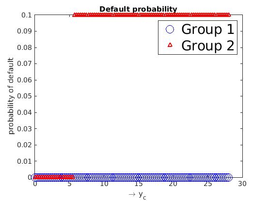
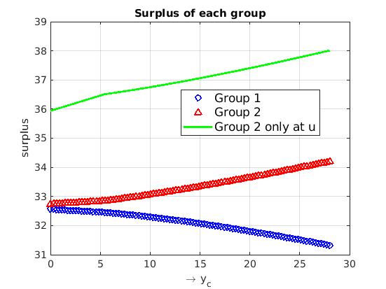
(a) $u=.5$ , $d=-.35$, $d_{c}=.1$, $\kappa=.175$, with, $d_{c}+\kappa=.275<\Delta_{r}=.295<\Delta_{u}=.38$

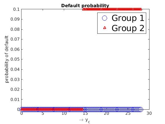
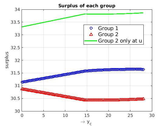
(b) $u=.5$ , $d=-.15$, $d_{c}=.1$, $\kappa=.245$, with, $\Delta_{r}=.315<d_{c}+\kappa=.345<\Delta_{u}=.38$

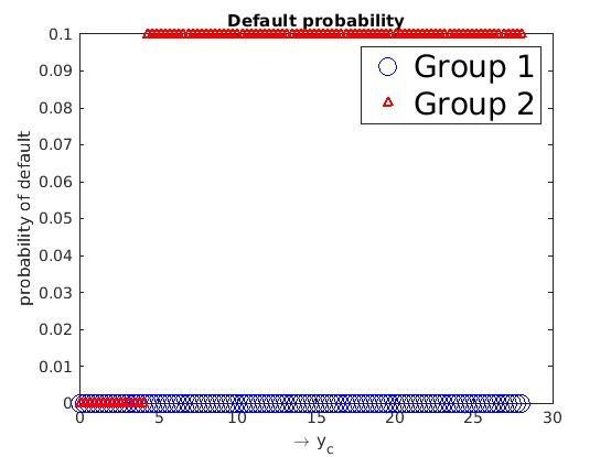
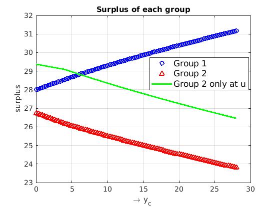
(c) $u=.5$ , $d=-.2$, $d_{c}=.1$, $\kappa=.35$, with, $\Delta_{r}=.31<\Delta_{u}=.38<d_{c}+\kappa=.45$

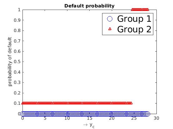
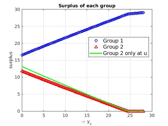
(d) $u=.5$ , $d=-.01$, $d_{c}=.1$, $\kappa=.77$, with, $\Delta_{r}=.329<\Delta_{u}=.38<d_{c}+\kappa=.87$

Figure 4: Small shock regime: $w=.1$, $r_{1}=.1$, $r_{2}=.12$, $p^{sb}_{2}=.2$, $p^{sb}_{1}=.01$.

We have used the following common set of parameters for our numerical examples: $k_{0}=40/(1+u-d_{c})$, $k_{b}=50/(1+u-d_{c})$, $y_{1}=50/(1+r_{1})$, $y_{2}=50/(1+r_{2})$, $\bar{y}_{1}=y_{1}(1+r_{1})$, $\bar{y}_{2}=(y_{2}+y_{c})(1+r_{2})$, $\gamma=0.5$ and the rest of the system parameters are given in the captions of the respective figures. In Figure 4 (and its sub-figures), we consider small shock regime ($v_{2}<k_{d2}$), while, Figure 6 studies the large shock regime ($v_{2}>k_{d2}$).

Moderate and small shock regime ($v_{2}<k_{d2}$): Lemma 8 characterizes the trends in the performance under resilient regime (which is possible only under small-shock regime); and interestingly the trends continue even in default regime (when $P^{2}_{D}>0$) for the case with small-shocks:

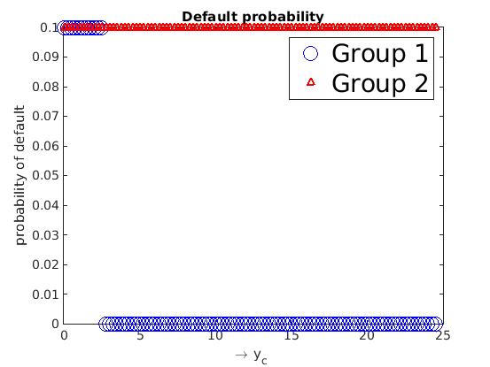
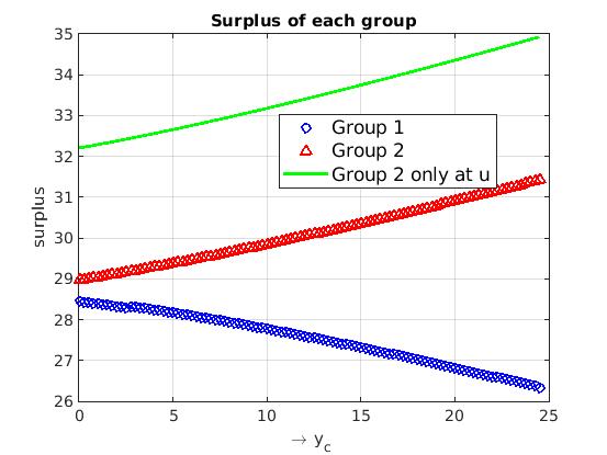
(a) $u=.7$ , $d=-.7$, $d_{c}=.1$, $\kappa=.32$, with, $d_{c}+\kappa=.42<\Delta_{r}=.44<\Delta_{u}=.58$

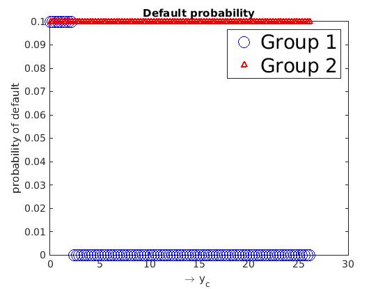
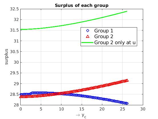
(b) $u=.6$ , $d=-.7$, $d_{c}=.1$, $\kappa=.3$, with, $\Delta_{r}=.35<d_{c}+\kappa=.4<\Delta_{u}=.48$

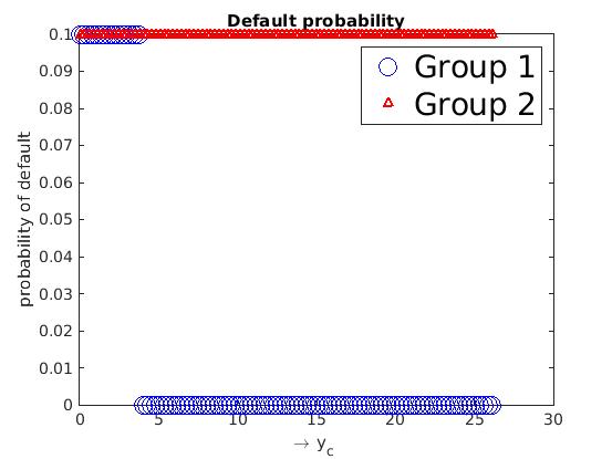
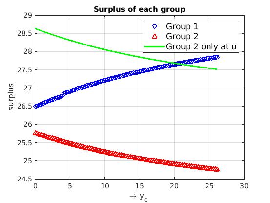
(c) $u=.6$ , $d=-.7$, $d_{c}=.1$, $\kappa=.375$, with, $\Delta_{r}=.35<d_{c}+\kappa=.475<\Delta_{u}=.48$

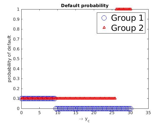
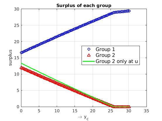
(d) $u=.4$ , $d=-.7$, $d_{c}=.1$, $\kappa=0.65$, with, $\Delta_{r}=.17<\Delta_{u}=.28<d_{c}+\kappa=.75$

Figure 6: Large shock regime: $w=.1$, $r_{1}=.1$, $r_{2}=.12$, $p^{sb}_{2}=.2$, $p^{sb}_{1}=.01$.

1. When, $\Delta_{r}$, the difference in the expected rate of return from risky assets and the rate $r_{2}$ of liabilities of group ${\cal G}_{2}$ is smaller than the system ‘burden factor’ $d_{c}+\kappa$, then the expected surplus of ${\cal G}_{1}$ banks improves with increase in $y_{c}$ (see figures (4(b)), (4(c)), (4(d))). Moreover, this trend continues in default regime also.

2. On the other hand, if $\Delta_{u}$ (the difference between upward rate and $r_{2}$) is bigger than $d_{c}+\kappa$, then SaU of group ${\cal G}_{2}$ improves with $y_{c}$ as seen in figures (4(a)) and (4(b)). This trend also continues in the default regime.

3. For the case study of figure (4(b)), both the groups improve; SaU as well as $E[S_{1}]$ increase with $y_{c}$, even in default regime.

4. When $\Delta_{r}>d_{c}+\kappa$, $E[S_{1}]$ decreases, while, $E[S_{2}]$ as well as the SaU of ${\cal G}_{2}$ banks improves with $y_{c}$ (figure (4(a))). While with $d_{c}+\kappa>\Delta_{u}$, only group 1 improves (figures (4(c)), (4(d))). These trends also continue (even with $P_{D}^{2}=1$).

Large shock regime ($v_{2}>k_{d2}$): This regime is considered in Figure 6. The observations are almost similar to that in the previous case, except for the switch-over points: a) when $d_{c}+\kappa$ is small, only group 2 banks benefit; b) with larger burden factor, both the groups benefit; c) when the burden factor is increased further, only group 1 banks benefit with increase in $y_{c}$; and d) the switch over points of $d_{c}+\kappa$ for above three types of regimes are given in Lemma 8, are valid even in default regime with small shocks; however e) the switch-over points can be different with larger shocks (see figure (6(c))).

7 Monte Carlo Simulations

In the previous sections, we derived asymptotic performance and systemic-risk analysis of a financial network using the fixed-point convergence theorems of Section 2 and 3. This section reinforces the approximation demonstrated by Theorem 4, using exhaustive Monte-Carlo (MC) simulations. Alongside, we discuss the rate of convergence, which in turn discusses the accuracy of the convergence result for the smaller (and practical) number of entities.

We consider an example system with $\gamma=0$, i.e., with one group in this section. For each run of the simulation, we first generate a realization of the random graph by generating independent binary random variables (with probability $p_{2}$) $\{I_{j,i}\}$ for all $j,i$ and another set of independent binary random variables (with probability $p_{2}^{sb}$) $\{\eta_{j}^{sb}\}$ for all $j$, also independent of the former set. Thus we have a realization of the financial network along with the portfolios of each entity. We then generate the realization of economic shocks by generating the two-valued random variables with upward movement $u$ (with probability $(1-w)$) or downward movement $d$.

For each random sample generated as above, we compute $\{W_{j,i}\}$, $\{\Omega_{j}^{2}\}$ (as in (90)) and $\{K^{2}_{i}\}$ and solve the fixed point equations given in (96), (with $y_{c}=0$) to obtain the clearing vector $\{X_{i}\}_{i}$. The corresponding fixed point equation modifies to the following with $\gamma=0$ (with ${\bf X}:=(X_{1},\cdots,X_{n})$):

$$f_{i}({\bf X}) := \min\bigg{\{}\bigg{(}K^{2}_{i}+\ \displaystyle\sum_{j\in\mathcal{G}_{2}}X_{j}W_{j,i}-v_{2}\bigg{)}^{+},\bar{y}_{2}\bigg{\}},\mbox{ for any }~{}i.\mbox{ where, }$$ (119)

$$K^{2}_{i} = \begin{cases}k_{u2}&\text{with probability }\ 1-w\\ k_{d2},&\text{otherwise,}\mbox{ with }k_{u2}=\Omega_{i}^{2}(1+u)\mbox{ and }k_{d2}=\Omega_{i}^{2}(1+d).\end{cases}$$

In particular we are considering the scenarios with $P^{2}_{D}=w$ and $v_{2}>k_{d2}$ for this case-study; under these conditions by Lemma 5 (case 3) we have:

$${\bar{x}}_{th} = \frac{{\bar{y}}_{2}(1-w)+(k_{d2}-v_{2})w}{1-w(1-p_{2}^{sb})}(1-p_{2}^{sb}),$$ (120)

$$E[S]_{th} = (k_{u2}-v_{2}+{\bar{x}}_{th}-{\bar{y}}_{2})(1-w).$$ (121)

Throughout the simulations, we use the following set of common parameters, and any additional changes of the parameters are mentioned in the respective table itself: $u=0.2$, $d=-0.6$, $r_{2}=0.12$, $\kappa=0.56$, $\Omega_{2}=12.5$, $\bar{y}_{2}=35$, $v_{2}=7$, $w=0.2$, $p_{2}^{sb}=0.001$, $y_{c}=0$, $d_{c}=0$.

We use an iterative algorithm to minimize $\sum_{i\leq n}\left(X_{i}-f_{i}({\bf X})\right)^{2}$ (observe FP is the minimizer) to obtain the fixed point, i.e., the clearing vector of any sample path. The same is provided in Algorithm 1.

Algorithm 1 Fixed-point algorithm to compute the clearing vector

1:Inputs: $n$, $k$, $K_{i}^{2}$, $\{W_{j,i}\}$, $\bar{y}_{2}$, $v_{2}$, $\delta$, $T$.

2:Initialize $X^{0}_{i}={\bar{y}}_{2}$ for all $i\leq n$

3:Iteration: $t=1,2,\cdots T$

4:a: update: $X_{i}^{t+1}=X_{i}^{t}-\epsilon_{t}(f_{i}({\bf X}^{t})-X_{i}^{t})$

5:b: if $\sum_{i=1}^{n}|X_{i}^{s+1}-X_{i}^{s}|<n\delta$, for all $s=t-k,t-k+1,\cdots,t$

6:c: algorithm converged and end

7:end

$n$	$\bar{x}_{th}$	$\widehat{\bar{x}}$	Error($\%$)	$E[S]_{th}$	$\widehat{E}[S]$	Error($\%$)
600	34.5	34.2414	0.7496	6	5.9036	1.6061
700	34.5	34.2760	0.6493	6	5.9551	0.7484
800	34.5	34.3653	0.3904	6	5.9717	0.4722
900	34.5	34.4262	0.2139	6	6.0245	0.4078
1000	34.5	34.4395	0.1754	6	6.0267	0.4452

Table 1: Sample path wise estimates for ER-graphs.

Once we ensure the convergence of the estimates in the algorithm (when the difference of step 3(b) of Algorithm 1 is below $\delta=0.0001$ for $k=100$ consecutive steps), we compute the performance measures related to the systemic risk. We tabulate these estimates (represented using $\widehat{\cdot}$), along with aggregate fixed point in Table 1. We also tabulate the theoretical $\bar{x}_{th}$ (computed using (120)) and the theoretical expected surplus $E[S]_{th}$ (computed using (121)) in the same table. We further included an index by name “Error(%)” that compares the two sets by computing the normalized error as below, for example for expected surplus:

$$\frac{|E[S]_{th}-\widehat{E}[S]|}{E[S]_{th}}\times 100\%$$

Our theoretical results well-match the Monte-Carlo estimates (sample path-wise), even with a few hundred banks in the network. Observe here that the table is for one sample path of the graph model.

Random Graphs: In the previous example we considered only Erdős-Rényi (ER) graphs. For these graphs the generated sample paths are highly irregular, i.e., the variance in the number of connections (e.g., $\sum_{i}{I}_{j,i}$ is the number of lenders and $\sum_{i}{I}_{i,j}$ is the number of borrowers for entity $j$) across different entities of the network is high. Thus, we include another set of regular graphs. We generated the (correlated) regular graphs by discarding the samples if the number of connections deviated significantly from the true average. Such a controlled generation of the random graphs leads to more regular graphs with lesser variations in the number of lenders of various entities of each sample path. For example, with $np_{2}=500\times 0.05=25$, we allowed $\pm 2$ variations in the number of lenders. Observe here that the variations in the number of borrowers is still significantly high.

	Regular		ER		Regular		ER
	$p_{2}$=0.03				$p_{2}$=0.05
n	${\widehat{P}}^{2}_{D}$	CI	${\widehat{P}}^{2}_{D}$	CI	${\widehat{P}}^{2}_{D}$	CI	${\widehat{P}}^{2}_{D}$	CI
500	0.1795	0.0038	0.1397	0.0087	0.1896	0.0029	0.1499	0.0074
1000	0.1898	0.0021	0.1517	0.0069	0.1973	0.0018	0.1612	0.0056
2000	0.1986	0.0013	0.1642	0.0051	0.1990	0.0014	0.1752	0.0036
5000	0.2001	0.0008	0.1850	0.0022	0.2000	0.0008	0.1937	0.0012

Table 2: Default-probability estimates over $200$ sample paths.

	Regular		ER		Regular		ER
	$p_{2}=0.03$				$p_{2}=0.05$
n	$\widehat{E}[S]$	CI	$\widehat{E}[S]$	CI	$\widehat{E}[S]$	CI	$\widehat{E}[S]$	CI
500	5.9680	0.0254	5.9715	0.0298	5.9713	0.0249	5.9520	0.0297
1000	5.9878	0.0162	5.9564	0.0182	5.9656	0.0179	5.9668	0.0168
2000	5.9606	0.0125	5.9709	0.0128	5.9724	0.0137	5.9784	0.0131
5000	5.9642	0.0084	5.9637	0.0070	5.9657	0.0076	5.9655	0.0081

Table 3: Expected-surplus estimates over $200$ sample paths.

We consider more sample paths in the next case-study in Tables 3-3. We estimated the default probability (${\widehat{P}}^{2}_{D}$) and the expected surplus ($\widehat{E}[S]$) for both ER and regular graphs by averaging over $200$ sample paths. When the number of banks is small for ER graphs, the error between the estimated default probability and the theoretical default probability ($P_{D}^{2}=w=0.2$) is significantly high. However the error reduces with the increase in the number of banks. Thus for ER graphs, the rate of convergence of the performance is slow. On the other hand, the same error is significantly small for regular graphs. Further the expected surplus and the aggregate clearing vector MC-estimates are close to the theoretical ones (provided in Table 1), even for small values of $n$ and even for ER graphs (see Table 3). We tabulated only $\widehat{E}[S]$ estimates, as the error/difference is significantly small for one sample path itself as in Table 1.

Confidence intervals: It is a standard practice to compute the $95\%$ confidence interval by estimated-mean $\pm$ Half-width ($H_{W}$) of the estimated performance, where, $H_{W}$:=1.96 $\times$ $\sqrt{variance}/\sqrt{\#samples}$. For simpler representation, in all the tables (Table 3-4), $H_{W}$ is shown as the confidence interval (CI). Once again regular graphs have good CIs even for small values of $n$, while ER graphs are good only for larger $n$. However the CIs related to expected surplus (in Table 3) are very good for both the types of graphs. Further CIs are better with bigger probability of connection $p_{2}$; and so are the estimated means.

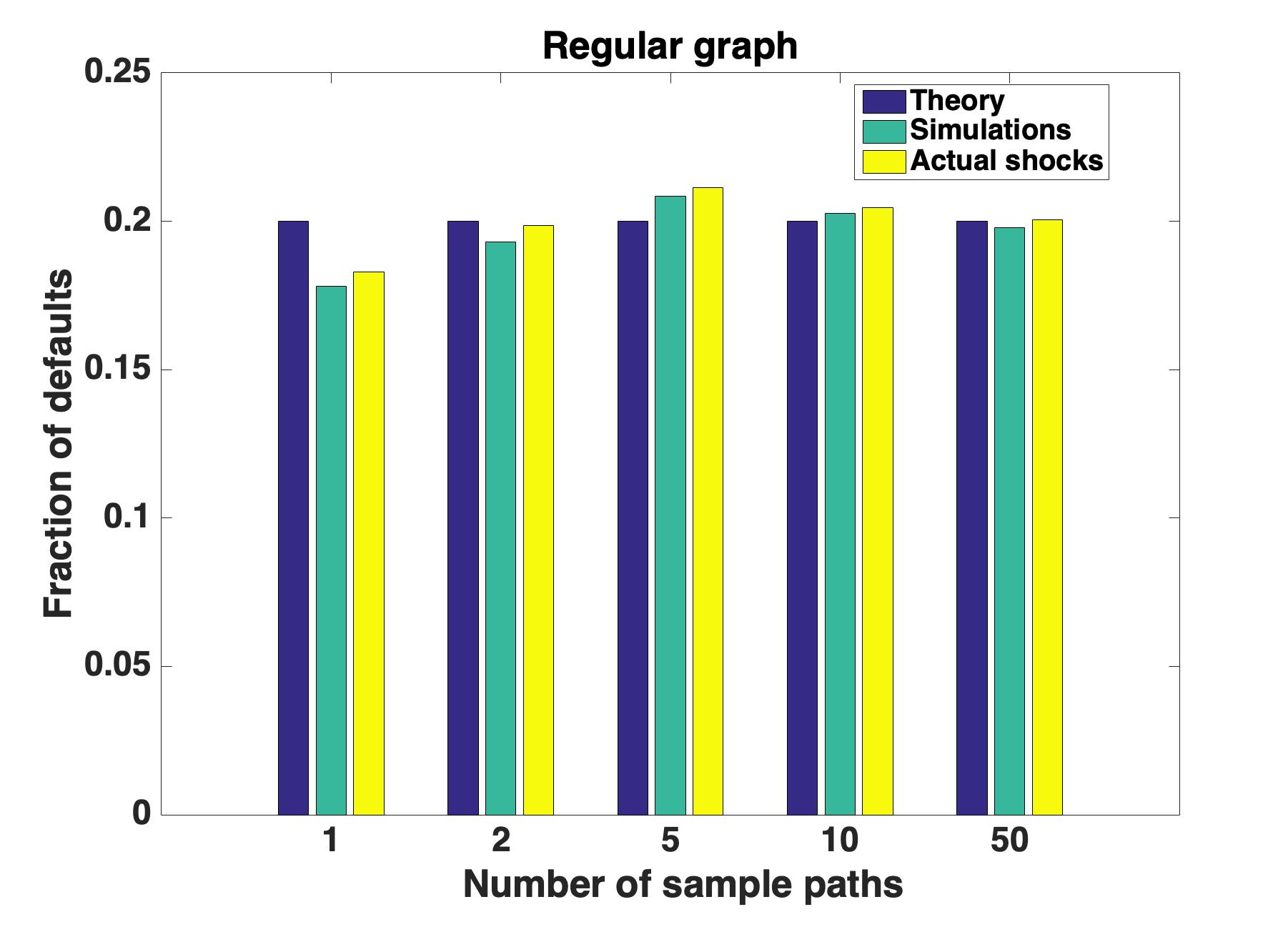
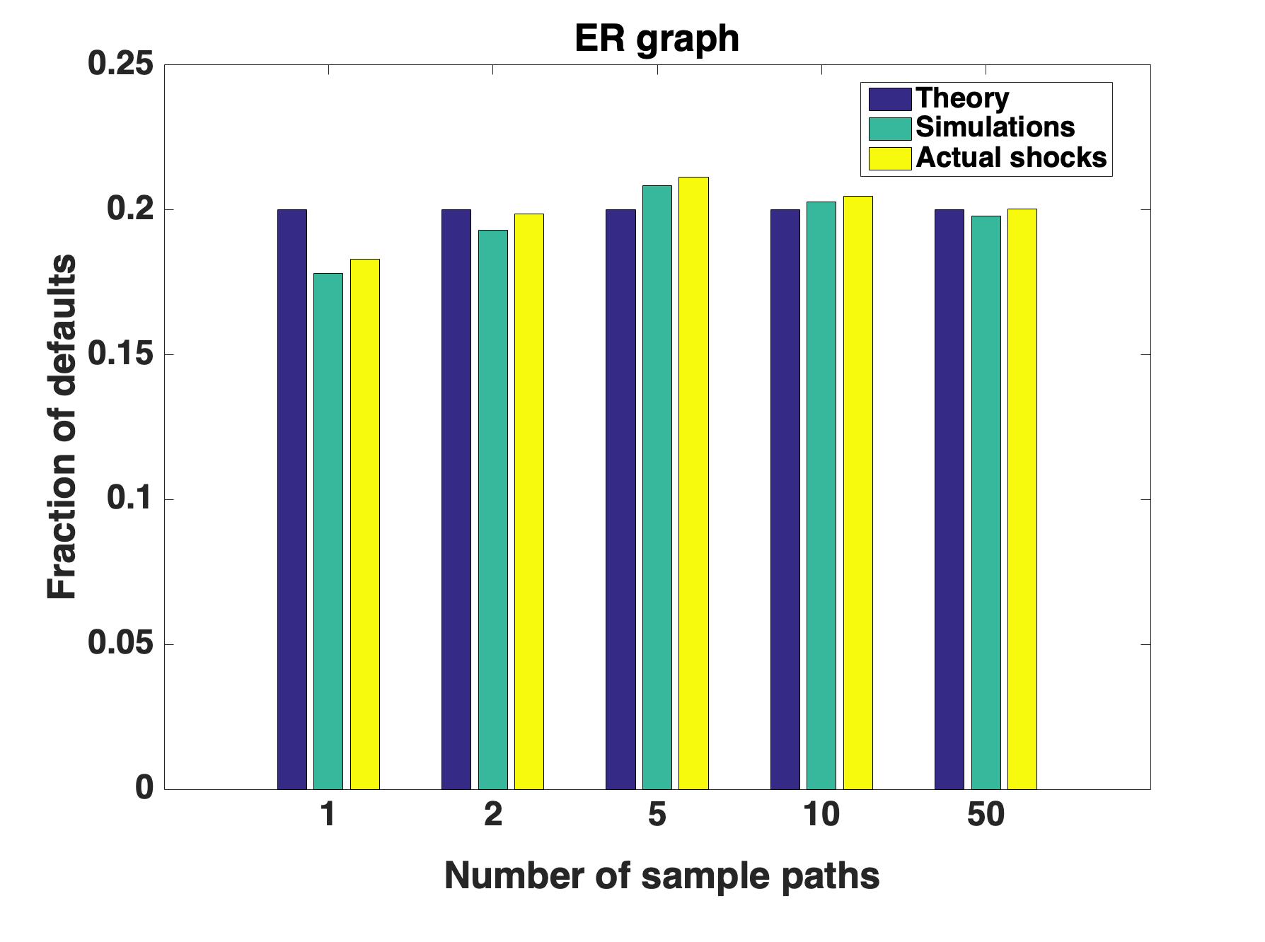
Figure 8: Few sample-path estimates with $n=1000$: fraction of defaults and fraction of banks with shocks.

In the bar charts of Figure 8, we consider another case-study with small number of sample paths for default probability estimates. We consider average over $1,2,5,10$ and $50$ sample paths. The figure represents the theoretical default probability, simulated default probability, and the fraction of banks that receive the shocks for the regular graph (left sub-figure) and the ER graph (right sub-figure). The correlation between the simulated fraction of defaults and the simulated fraction of banks that received the shocks is higher in regular graphs, than that in ER graph. Nevertheless, in both the graphs there is good correlation between these two estimates, and both of them converge closer to theoretical estimate $w=0.2$ when the average is over large number of sample paths (more than or equal to $10$). The theory indicates that, for the conditions of these case-studies, the number of defaults should equal the number of the banks that received the shocks and the same is well correlated in the simulations, even when the actual fraction of defaults is away from $0.2$.

$n$	$\widehat{\bar{x}}$	${\widehat{P}}^{2}_{D}$	CI	$\widehat{E}[S]$	CI
200	34.3821	0.1635	0.0062	5.9816	0.0375
300	34.4105	0.1644	0.0059	5.9871	0.0351
400	34.4327	0.1831	0.0038	5.9455	0.0283

Table 4: Regular graphs performance estimates over $200$ sample paths.

Finally we consider further regular graphs, whose number of borrowers is also controlled and with even smaller number of agents in Table 4. With $n=200$, $300$ and $400$ we respectively allowed number of borrowers to be distributed between $10\pm 6$, $15\pm 9$ and $20\pm 12$, while the number of lenders is distributed respectively between $10\pm 1$, $15\pm 2$ and $20\pm 2$. We observe a sufficiently good match between theoretical values and the corresponding MC estimates, even for these small values of $n$. We thus conclude that our theoretical estimates are sufficiently good matches even for few hundreds of banks when the number of connections across agents is not too diverse. Thus our results can provide a good method for estimating clearing vectors and further systemic-risk measures for many practical scenarios.

8 Conclusions

We consider a large dimensional fixed point equation, where the function corresponding to any component depends upon a weighted aggregate of the values of its random neighbours. The underlying fixed point equations are random, and we provide a methodology to solve such equations under suitable graph structure(s); our main contribution is to solve these equations almost surely. We consider two different types of random graph models: the resources are shared equally across the (connected components of the) entire network in the first model. In contrast, in the second model, the resources are shared equally only within the group after allocating dedicated fractions to each group. In both the models, the solution of the random fixed point equation converges almost surely to that of a limit system, and these solutions are asymptotically independent. This asymptotic simplification reduced the dimensionality of the problem significantly; the almost-sure asymptotic solution is derived by solving a deterministic three-dimensional fixed point equation.

We apply the above results to a large financial network to study systemic risk related aspects. In such networks, the first object to be studied is clearing vector, a vector of maximum possible repayments (towards clearing their liabilities) by all the nodes of the network; this vector depends upon the random economic shocks received by a fraction of agents, and the percolation of the influence of these shocks on the clearing capacity of their neighbours, neighbours of neighbours and so on. One of our primary results is a procedure to compute clearing vector of a variety of large-dimensional financial networks; in the example considered in this paper, solution of a two-dimensional deterministic fixed point equation is sufficient to study the clearing vector.

Considering a heterogeneous financial network with two-period framework, binomial shocks and with two diverse groups (one aggressive to consider more risky avenues while the other is recessive), we derived systemic-risk based performance measures, after deriving the clearing vectors. For majority of the cases, closed-form expressions are obtained for aggregate clearing vector, systemic risk performance measures viz. probability of default and expected surplus; for other cases we solved the two-dimensional equations numerically. In the limiting network, we observed some phase transitions with respect to inter group-connectivity parameters: a) the existence of a regime of connectivity parameters, wherein the surplus of both the groups improves with the parameters; and b) in large shock regimes, the inter-connectivity has adverse effect, at least on one of the groups.

We performed exhaustive Monte-Carlo simulations using practical number of financial entities and Erdős-Rényi graphs with an aim to study the accuracy of approximation. We observed good match for the surplus based performance measures and clearing vectors, even with few hundreds of banks. With more regular graphs (smaller variations in the number of connected components) there is a good match even between default probability estimates and their theoretical counterparts.

Appendix A: Proofs related to Section 2, random fixed points

Proof of Lemma 2: First consider the term $\frac{1}{n}\sum_{j\in\mathcal{G}_{1}}\xi^{1}_{j}({\bar{x}}^{1}_{j},x_{b})W_{j,b}$ (recall $x_{b}=f^{b}({\bar{x}}_{b})$ is deterministic). Now consider the constant sequences $({{\bar{\bf x}}}^{1},{{\bar{\bf x}}}^{2})$, i.e., $\bar{x}_{j}^{m}=\bar{x}^{m}$ (same for all $j\in\mathcal{G}_{m}$) for each $m\in\{1,2\}$. Then $\{\xi^{1}_{j}({\bar{x}}^{1},x_{b})W_{j,b}\}_{j}$ is an i.i.d. sequence of random variables (see (2) and (14)) and by law of large numbers (note $E[W_{j,b}]=p_{1}^{sb}$ for $j\in{\cal G}_{1}$)

$$\frac{1}{n}\sum_{j\in\mathcal{G}_{1}}\xi^{1}_{j}({\bar{x}}^{1}_{j},x_{b})W_{j,b}\to{\gamma}E_{G^{1}_{i},\eta_{i}^{bs}}[\xi^{1}_{i}({\bar{x}}^{1},x_{b})]p_{1}^{sb}\mbox{ a.s., as }n\to\infty\ \ (\mbox{for any }i).$$

Similarly, $\frac{1}{n}\sum_{j\in\mathcal{G}_{2}}\xi^{2}_{j}({\bar{x}}^{2}_{j},x_{b})W_{j,b}\to(1-\gamma)E_{G^{2}_{i},\eta_{i}^{bs}}[\xi^{2}_{i}({\bar{x}}^{2},x_{b})]p_{2}^{sb}\mbox{ a.s. }$

From (18), the aggregate (fixed point) function, for constant sequences is:

$${\bar{f}}^{n,m}_{i}({\bar{x}}_{b},{\bar{x}}^{1},{\bar{x}}^{2}) = \left\{\begin{array}[]{lll}\displaystyle\sum_{j\in\mathcal{G}_{1}}\xi^{1}_{j}({\bar{x}}^{1},x_{b})W_{j,i}+\displaystyle\sum_{j\in\mathcal{G}_{2}}\xi_{j}^{2}({\bar{x}}^{2},x_{b}){W}_{j,i}&\mbox{ if }i\in\mathcal{G}_{m}\\ 0&\mbox{ else}\end{array}\right.$$ (124)

Fix any $i\in\mathcal{G}_{m^{\prime}}$. Define $M^{m}_{j}=\xi^{m}_{j}({\bar{x}}^{m},x_{b})I_{j,i}$ and observe these are i.i.d. random variables for each $m$, uniformly bounded by constant $y$ of B.1. By Lemma 9, each term of (124) converges in almost sure sense on set ${\cal E}$ of B.2 to the following:

$$\sum_{j\in\mathcal{G}_{m}}\xi^{m}_{j}({\bar{x}}^{m}x_{b})W_{j,i}\to E_{G^{m}_{i},\eta_{i}^{bs}}\left[\xi^{m}_{i}({\bar{x}}^{m},x_{b})\right]p_{mm^{\prime}}\gamma_{m}\frac{(1-p^{sb}_{m})}{\gamma_{p_{m}}}.$$

Adding over all possible $m,m^{\prime}\in\{1,2\}$ we have the desired convergence. $\blacksquare$

Lemma 9

Assume B.2(C). Consider an i.i.d. sequence $\{M_{j}\}$,which is uniformly bounded by some constant $c_{0}<\infty$. Define the following random variables, one for each $n$ and for any $i\in\mathcal{G}_{m^{\prime}}$ $m,m^{\prime}\in\{1,2\}$ as below (see equation (2)):

$${\zeta}^{n}:=\sum_{j\in\mathcal{G}_{m}}M_{j}W_{j},\ \ {\tilde{\zeta}}^{n}:=\sum_{j\in\mathcal{G}_{m}}I_{j,i}M_{j}W_{j}\ \mbox{ with }W_{j}:=\frac{(1-\eta_{j}^{sb})}{\displaystyle\sum_{i^{\prime}\leq n}I_{j,i^{\prime}}}.$$

i) we have the following convergence (${\cal E}$ defined in equation (13))

$${\zeta}^{n}\to E[M_{j}]\gamma_{m}\frac{1-p^{sb}_{m}}{\gamma_{{}_{p_{m}}}}\mbox{, }\ \ {\tilde{\zeta}}^{n}\to E[M_{j}]p_{m^{\prime}m}\gamma_{m}\frac{1-p^{sb}_{m}}{\gamma_{{}_{p_{m}}}}\mbox{ a.s. on set, }{\cal E};\mbox{ and, }$$

ii) Under B.2, the above convergence is w.p.1.

Proof: By adding and subtracting appropriate terms and from the equation (2):

$$\bigg{|}{\zeta}^{n}-E[M_{j}]\gamma_{m}\frac{1-p^{sb}_{m}}{\gamma_{{}_{p_{m}}}}\bigg{|} = \bigg{|}\sum_{j\in\mathcal{G}_{m}}M_{j}W_{j}-\sum_{j\in\mathcal{G}_{m}}M_{j}\frac{(1-\eta_{j}^{sb})}{n\gamma_{{}_{p_{m}}}}+\sum_{j\in\mathcal{G}_{m}}M_{j}\frac{(1-\eta_{j}^{sb})}{n\gamma_{{}_{p_{m}}}}-E[M_{j}]\gamma_{m}\frac{1-p^{sb}_{m}}{\gamma_{{}_{p_{m}}}}\bigg{|}$$

$$=\ \bigg{|}\sum_{j\in\mathcal{G}_{m}}M_{j}\frac{(1-\eta_{j}^{sb})}{\displaystyle\sum_{i^{\prime}\in\mathcal{G}_{1}\cup\mathcal{G}_{2}}I_{j,i^{\prime}}}-\sum_{j\in\mathcal{G}_{m}}M_{j}\frac{(1-\eta_{j}^{sb})}{n\gamma_{{}_{p_{m}}}}+\sum_{j\in\mathcal{G}_{m}}M_{j}\frac{(1-\eta_{j}^{sb})}{n\gamma_{{}_{p_{m}}}}-E[M_{j}]\gamma_{m}\frac{1-p^{sb}_{m}}{\gamma_{{}_{p_{m}}}}\bigg{|}$$

$$\leq\ \bigg{|}\sum_{j\in\mathcal{G}_{m}}M_{j}(1-\eta_{j}^{sb})\bigg{(}\frac{1}{{\sum_{i\in\mathcal{G}_{1}\cup\mathcal{G}_{2}}I_{j,i}}}-\frac{1}{n\gamma_{{}_{p_{m}}}}\bigg{)}\bigg{|}+\bigg{|}\sum_{j\in\mathcal{G}_{m}}M_{j}\frac{(1-\eta_{j}^{sb})}{n\gamma_{{}_{p_{m}}}}-E[M_{j}]\gamma_{m}\frac{1-p^{sb}_{m}}{\gamma_{{}_{p_{m}}}}\bigg{|}$$

$$\leq\ \sum_{j\in\mathcal{G}_{m}}c_{0}\bigg{|}\bigg{(}\frac{1}{{\sum_{i\in\mathcal{G}_{1}\cup\mathcal{G}_{2}}I_{j,i}}}-\frac{1}{n\gamma_{{}_{p_{m}}}}\bigg{)}\bigg{|}+\bigg{|}\sum_{j\in\mathcal{G}_{m}}M_{j}\frac{(1-\eta_{j}^{sb})}{n\gamma_{{}_{p_{m}}}}-E[M_{j}]\gamma_{m}\frac{1-p^{sb}_{m}}{\gamma_{{}_{p_{m}}}}\bigg{|}$$

$$\xrightarrow[\text{B.2 and LLN}]{n\to\infty}0\mbox{ a.s. on set ${\cal E}$ of {\bf B.2}.}\hskip 28.45274pt$$

The proof for ${\tilde{\zeta}}^{n}$ goes through in a similar way when $\{I_{j,i}\}$ are i.i.d. Otherwise it still goes through because of the following modified steps (in addition to the previous steps).

$$\bigg{|}\sum_{j\in\mathcal{G}_{m}}M_{j}I_{j,i}\frac{(1-\eta_{j}^{sb})}{n\gamma_{{}_{p_{m}}}}-E[M_{j}]p_{m^{\prime},m}\gamma_{m}\frac{1-p^{sb}_{m}}{\gamma_{{}_{p_{m}}}}\bigg{|} \leq \bigg{|}\sum_{j\in\mathcal{G}_{m}}M_{j}I_{j,i}\frac{(1-\eta_{j}^{sb})}{n\gamma_{{}_{p_{m}}}}-\sum_{j\in\mathcal{G}_{m}}M_{j}p_{m^{\prime},m}\frac{(1-\eta_{j}^{sb})}{n\gamma_{{}_{p_{m}}}}\bigg{|}$$

$$+\bigg{|}\sum_{j\in\mathcal{G}_{m}}M_{j}p_{m^{\prime},m}\frac{(1-\eta_{j}^{sb})}{n\gamma_{{}_{p_{m}}}}-E[M_{j}]p_{m^{\prime},m}\gamma_{m}\frac{1-p^{sb}_{m}}{\gamma_{{}_{p_{m}}}}\bigg{|}$$

$$\leq \frac{c_{0}}{\gamma_{{}_{p_{m}}}}\bigg{|}\sum_{j\in\mathcal{G}_{m}}\frac{I_{j,i}}{n}-\sum_{j\in\mathcal{G}_{m}}\frac{p_{m^{\prime},m}}{n}\bigg{|}$$

$$+\bigg{|}\sum_{j\in\mathcal{G}_{m}}M_{j}p_{m^{\prime},m}\frac{(1-\eta_{j}^{sb})}{n\gamma_{{}_{p_{m}}}}-E[M_{j}]p_{m^{\prime},m}\gamma_{m}\frac{1-p^{sb}_{m}}{\gamma_{{}_{p_{m}}}}\bigg{|}$$

$$\to 0\mbox{ a.s.}$$

because of assumption B.2(C) and law of large numbers. $\blacksquare$

Appendix B: Proof of Theorem 1

Proof of Theorem 1: We consider the following norm for this proof on the space of infinite sequences, $[0,y]\times s^{\infty}\times s^{\infty}$:

$$||({\bar{x}}_{b},{\bar{\bf x}})-({\bar{u}}_{b},{\bar{\bf u}})||_{\infty} = \max_{m\in\{1,2\}}\sup_{i\in\mathcal{G}_{m}}\left(|\bar{x}^{m}_{i}-\bar{u}^{m}_{i}|+|{\bar{x}}_{b}-{\bar{u}}_{b}|\right)$$ (126)

From the equations (14)-(15) and assumption B.1, the finite $n$-systems have aggregate fixed points (in almost sure sense), using Brouwer’s fixed point Theorem. Further the limit system has (aggregate) fixed point as given by assumption B.5. Thus we define the following function whose zeros are the fixed points of the mappings ${\bar{\bf f}}^{n,m}$ given by (18) for any $n\leq\infty$; define ${\cal N}=\{1,2,\cdots,\infty\}$ and define the real valued function $h(\cdot)$ from $\left([0,y]\times s^{\infty}\times s^{\infty}\right)\times{\cal N}\to{\cal R}^{+}$ as below (recall $|{\cal G}_{1}|+|{\cal G}_{2}|=n$)

$$h({\bar{x}}_{b},{\bar{\bf x}},n) = |{\bar{f}}^{n}_{b}({\bar{x}}_{b},{\bar{\bf x}})-{\bar{x}}_{b}|+\sum_{m=1}^{2}\left(\sum_{i\in\mathcal{G}_{m}}2^{-i}|{\bar{f}}^{n,m}_{i}({\bar{x}}_{b},{\bar{\bf x}})-{\bar{x}}^{m}_{i}|+\sum_{i>n}2^{-i}{\bar{x}}_{i}^{m}\right)$$

$$h({\bar{x}}_{b},{\bar{\bf x}},\infty) = \left(|{\bar{f}}^{\infty}_{b}({\bar{x}}_{b},{\bar{\bf x}})-{\bar{x}}_{b}|+\sum_{m=1}^{2}\sum_{i\in\mathcal{G}_{m}}2^{-i}|{\bar{f}}^{\infty,m}_{i}({\bar{x}}_{b},{\bar{\bf x}})-{\bar{x}}^{m}_{i}|\right).$$

It is clear that the aggregate fixed points form the minimizers of the above functions. Our idea is to obtain the convergence proof using continuity of optimizers as given by Maximum Theorem (e.g., [6, 19, 12]). Towards this we begin with joint continuity of the objective function.
Joint continuity: We require some (sample path-wise) inequalities for showing the joint continuity of the objective function and we begin with the same. Towards this, we consider the set ${\cal C}$ of Corollary 3 (provided later in the same Appendix). By Corollary 3 (under assumption B.2), $P({\cal C})=1$ and for any $w\in{\cal C}$, there exists an $N_{w}<\infty$ such that for all $n\geq N_{w}$:

$$\frac{1}{n}\sum_{j\in\mathcal{G}_{1}}W_{j,b}+\frac{1}{n}\sum_{j\in\mathcal{G}_{2}}W_{j,b}\ \ \ \leq \ \ \ 2\gamma p_{1}^{sb}+2(1-\gamma)p_{2}^{sb}\mbox{\normalsize, and, }$$ (127)

$$\sum_{j\in\mathcal{G}_{1}}\frac{1-\eta_{j}^{sb}}{\sum_{i^{\prime}\in\mathcal{G}_{1}\cup\mathcal{G}_{2}}I_{j,i^{\prime}}}+\sum_{j\in\mathcal{G}_{2}}\frac{1-\eta_{j}^{sb}}{\sum_{i^{\prime}\in\mathcal{G}_{1}\cup\mathcal{G}_{2}}I_{j,i^{\prime}}} \leq \ \ \ 2\bigg{(}\frac{\gamma(1-p_{1}^{sb})}{\gamma_{{}_{p_{1}}}}+\frac{(1-\gamma)(1-p_{2}^{sb})}{\gamma_{{}_{p_{2}}}}\bigg{)}.\hskip 11.38109pt$$ (128)

Thus for all such $n$ we have from equation (2), as $I_{j,i}\leq 1$:

$$\sum_{i\in\mathcal{G}_{1}\cup{\mathcal{G}}_{2}}2^{-i}\sum_{m=1}^{2}\sum_{j\in\mathcal{G}_{m}}W_{j,i} \leq \sum_{i\in\mathcal{G}_{1}\cup{\mathcal{G}}_{2}}2^{-i}\bigg{(}\sum_{j\in\mathcal{G}_{1}}\frac{1-\eta_{j}^{sb}}{\sum_{i^{\prime}\in\mathcal{G}_{1}\cup\mathcal{G}_{2}}I_{j,i^{\prime}}}+\sum_{j\in\mathcal{G}_{2}}\frac{1-\eta_{j}^{sb}}{\sum_{i^{\prime}\in\mathcal{G}_{1}\cup\mathcal{G}_{2}}I_{j,i^{\prime}}}\bigg{)}$$ (129)

$$\leq \sum_{i\leq\infty}2^{-i}2\bigg{(}\frac{\gamma(1-p_{1}^{sb})}{\gamma_{{}_{p_{1}}}}+\frac{(1-\gamma)(1-p_{2}^{sb})}{\gamma_{{}_{p_{2}}}}\bigg{)}$$

$$=: 2c<\infty,$$

where, $c$ is an appropriate constant.

In the second step we will show that $h(.)$ is a Lipschitz continuous function in $({\bar{x}}_{b},{\bar{\bf x}})$ for all such $w\in{\cal C}$ and that the co-efficient of Lipschitz continuity can be the same for all $n\geq N_{w}$ and for $\infty$. For any $({\bar{x}}_{b},{\bar{\bf x}})$ and $({\bar{u}}_{b},{\bar{\bf u}})$, using Lipschitz continuity assumption B.3 (note $\varsigma\leq 1$), we have for all $n>N_{w}$ (see equation (15) and (126)):

$$|h({\bar{x}}_{b},{\bar{\bf x}},n)-h({\bar{u}}_{b},{\bar{\bf u}},n)|\hskip 28.45274pt$$ (130)

$$\leq\ \sum_{m=1}^{2}\sum_{i\in\mathcal{G}_{m}}2^{-i}|{\bar{f}}^{n,m}_{i}({\bar{x}}_{b},{\bar{\bf x}})-{\bar{f}}^{n,m}_{i}({\bar{u}}_{b},{\bar{\bf u}})|$$

$$+|{\bar{f}}^{n}_{b}({\bar{x}}_{b},{\bar{\bf x}})-{\bar{f}}^{n}_{b}({\bar{u}}_{b},{\bar{\bf u}})|+|{\bar{x}}_{b}-{\bar{u}}_{b}|+\ \sum_{m=1}^{2}\sum_{i\in\mathcal{G}_{m}}2^{-i}|{\bar{x}}^{m}_{i}-{\bar{u}}^{m}_{i}|+\sum_{i>n}2^{-i}|{\bar{x}}^{m}_{i}-{\bar{u}}^{m}_{i}|$$

$$\leq\ 2\sigma||({\bar{x}}_{b},{\bar{\bf x}})-({\bar{u}}_{b},{\bar{\bf u}})||_{\infty}\sum_{i\in\mathcal{G}_{1}\cup\mathcal{G}_{2}}2^{-i}\sum_{j\in\mathcal{G}_{1}\cup\mathcal{G}_{2}}W_{j,i}+2||({\bar{x}}_{b},{\bar{\bf x}})-({\bar{u}}_{b},{\bar{\bf u}})||_{\infty}\left(1+\sum_{i\in\mathcal{G}_{1}\cup\mathcal{G}_{2}}2^{-i}\right)$$

$$+2\sigma||({\bar{x}}_{b},{\bar{\bf x}})-({\bar{u}}_{b},{\bar{\bf u}})||_{\infty}\left(\frac{1}{n}\sum_{j\in\mathcal{G}_{1}}W_{j,b}+\frac{1}{n}\sum_{j\in\mathcal{G}_{2}}W_{j,b}\right)+||({\bar{x}}_{b},{\bar{\bf x}})-({\bar{u}}_{b},{\bar{\bf u}})||_{\infty}c^{\prime}$$

$$\leq\ 4||({\bar{x}}_{b},{\bar{\bf x}})-({\bar{u}}_{b},{\bar{\bf u}})||_{\infty}\left(c+\gamma p_{1}^{sb}+(1-\gamma)p_{2}^{sb}+1+\frac{c^{\prime}}{4}\right),$$

where $c^{\prime}$ is an appropriate constant. The above inequality is due to the bounds (127)-(129) and observe that the upper bound is uniform in $n$. Using exactly similar logic, we derive Lipschitz continuity for $n=\infty.$ By definition of limit system (20), when the limit superior becomes limit, we have:

$$|h({\bar{x}}_{b},{\bar{\bf x}},n)-h({\bar{x}}_{b},{\bar{\bf x}},\infty)|\to 0\mbox{ as $n\to\infty$}.$$

Thus and using (130), if $({\bar{x}}_{n,b},{\bar{\bf x}}_{n},n)\to({\bar{x}}_{b},{\bar{\bf x}},\infty)$, i.e., if $||({\bar{x}}_{n,b},{\bar{\bf x}}_{n})-({\bar{x}}_{b},{\bar{\bf x}})||_{\infty}\to 0$ as $n\to\infty$, with the limit $({\bar{x}}_{b},{\bar{\bf x}})\in{\cal\tilde{D}}$, where,

$${\cal\tilde{D}}:=\bigg{\{}({\bar{x}}_{b},{{\bar{\bf x}}})\in[0,y]\times s^{\infty}\times s^{\infty}:\mbox{ limit superior in \eqref{Eqn_bar_fixedpoint_limtGen 1} equals the limit}\bigg{\}},$$

then,

$$\hskip 2.84526pt|h({\bar{x}}_{n,b},{\bar{\bf x}}_{n},n)-h({\bar{x}}_{b},{\bar{\bf x}},\infty)|$$ (131)

$$\leq |h({\bar{x}}_{n,b},{\bar{\bf x}}_{n},n)-h({\bar{x}}_{b},{\bar{\bf x}},n)|+|h({\bar{x}}_{b},{\bar{\bf x}},n)-h({\bar{x}}_{b},{\bar{\bf x}},\infty)|\to 0.$$

This implies joint (norm) continuity of the function $h(.)$ on set ${\cal\tilde{D}}\times{\cal N}$, with ${\cal N}:=\{1,2,\cdots,\infty\}$. Observe that the fixed points of the finite systems (sequence has 0’s after finite $n$) and constant sequence are easily in ${\cal\tilde{D}}$ by Lemma 2, and hence by B.5 it suffices to consider minimizing $h(\cdot)$ over ${\cal\tilde{D}}$ to study the required fixed points.

We now apply Maximum Theorem for non-compact sets given by [12, Theorem 1.2] to complete the proof:

$\bullet$ We consider weak topology on $[0,y]\times s^{\infty}\times s^{\infty}$ generated by the set of projections, i.e., the smallest topology that ensures the ($m,i$)-th projection mapping $({\bar{x}}_{b},{\bar{\bf x}})\mapsto x^{m}_{i}$ from $[0,y]\times s^{\infty}\times s^{\infty}$ to ${\cal R}$ a continuous mapping for any $(m,i)$. This is basically the product topology and by the well known Tychonoff’s theorem, $[0,y]\times s^{\infty}\times s^{\infty}$ is a compact set under it.

$\bullet$ The set of the parameters ${\cal N}$ with topology as in footnote 10 is clearly compactly generated topological space;

$\bullet$ We have a constant correspondence $\Phi$: for any $n\in{\cal N}$ the domain is $\Phi(n)={\cal\tilde{D}}$;

$\bullet$ By definition of ${\cal\tilde{D}}$ and by (131) the function $h(\cdot,\cdot)$ is strong continuous on ${\cal\tilde{D}}$, and hence is weak continuous (under product topology); and

$\bullet$ Observe that for any compact set $K\subset{\cal N}$ the graph $Gr_{K}(\Phi)=K\times{\cal\tilde{D}}$ (definitions as in [12]). Consider the following level set,

$$\bigg{\{}(n,{\bar{x}}_{b},{\bar{\bf x}})\in K\times{\cal\tilde{D}}:h({\bar{x}}_{b},{\bar{\bf x}},n)\leq l\bigg{\}},\mbox{ for any compact set $K$ and level $l$.}$$

The above set is weak closed (by weak continuity of $h$) and hence is weak compact, as it is a subset of $K\times[0,y]\times s^{\infty}\times s^{\infty}$. Recall the domain ${\cal\tilde{D}}$ is a subset of weak (product) compact set $[0,y]\times s^{\infty}\times s^{\infty}$. Thus the function $h$ is $K$-inf compact on $Gr_{X}(\Phi)=X\times{\cal\tilde{D}}$ (definitions in [12]).

Thus by applying non-compact Maximum Theorem [12, Theorem 1.2] to the function $h(.)$ we obtain that the set of minimizers of $h(.)$ form a upper hemi-continuous (with respect to $n$) compact correspondence, under the product-topology ([6, 19]). By properties of upper hemi-continuous (with respect to $n$) compact correspondence ([6, 19]) we have the following result: a) consider any sequence of numbers $n_{k}\to\infty$ (it can also be $n\to\infty$); b) consider (any) one fixed point for each $n_{k}$, call it $\big{(}{\bar{x}}^{*}_{b}(n_{k}),{\bar{\bf x}}^{*}(n_{k})\big{)}$; c) then we have the following convergence along a sub-sequence $n_{k_{l}}\to\infty$ (under product topology):

$$\Big{(}{\bar{x}}^{*}_{b}(n_{k_{l}}),{\bar{\bf x}}^{*}(n_{k_{l}})\Big{)}\xlongrightarrow{\text{component-wise}}\Big{(}{\bar{x}}^{\infty*}_{b},{\bar{\bf x}}^{\infty*}\Big{)},$$

where $({\bar{x}}^{\infty*}_{b},{\bar{\bf x}}^{*})$ is a fixed point of the limit system. The last statement of the Theorem is immediate once we have the convergence of the aggregate fixed points, component-wise. $\blacksquare$

Corollary 3

The following set has measure 1 under the assumption B.2

$${\cal C}=\Big{\{}w:\frac{1}{n}\sum_{j\in\mathcal{G}_{1}}W_{j,b}(w)\stackrel{{\scriptstyle n\to\infty}}{{\to}}\gamma p_{1}^{sb},\frac{1}{n}\sum_{j\in\mathcal{G}_{2}}W_{j,b}(w)\stackrel{{\scriptstyle n\to\infty}}{{\to}}(1-\gamma)p_{2}^{sb}$$

$$\sum_{j\in\mathcal{G}_{1}}\frac{1-\eta_{j}^{sb}}{\sum_{i^{\prime}\in\mathcal{G}_{1}\cup\mathcal{G}_{2}}I_{j,i^{\prime}}}\to\frac{\gamma(1-p_{1}^{sb})}{\gamma_{{}_{p_{1}}}}\mbox{ and }$$

$$\sum_{j\in\mathcal{G}_{2}}\frac{1-\eta_{j}^{sb}}{\sum_{i^{\prime}\in\mathcal{G}_{1}\cup\mathcal{G}_{2}}I_{j,i^{\prime}}}\to\frac{(1-\gamma)(1-p_{2}^{sb})}{\gamma_{{}_{p_{2}}}}\Big{\}}.$$

Proof: It follows directly by law of large numbers (for the first two quantities of the set $\mathcal{C}$) and by Lemma 9 with $M_{j}\equiv 1$ (for the last two quantities). $\blacksquare$

Proof of Theorem 2: We consider finite $n$-system and consider the following norm for this proof:

$$||({\bar{\bf x}},{\bar{x}}_{b})||_{1}:=\frac{1}{n}\sum_{m}\sum_{j\in{\cal G}_{m}}\left(|x^{m}_{j}|+\varsigma|{\bar{x}}_{b})|\right)$$ (132)

Observe that for any $({\bar{x}}_{b},{\bar{\bf x}})$ (as $|{\cal G}_{1}|+|{\cal G}_{2}|=n$),

$$||{\bar{\bf f}}^{n}({\bar{x}}_{b},{\bar{\bf x}})||_{1}\ =\ \frac{1}{n}\sum_{m}\sum_{i\in{\cal G}_{m}}\left(|{\bar{f}}^{n,m}_{i}({\bar{x}}_{b},{\bar{\bf x}})|+\varsigma|{\bar{f}}^{n}_{b}({\bar{x}}_{b},{\bar{\bf x}})|\right)$$

$$= \frac{1}{n}\sum_{m}\sum_{i\in{\cal G}_{m}}\Bigg{(}\sum_{j\in\mathcal{G}_{1}}\xi^{1}_{j}({\bar{x}}^{1}_{j},x_{b})W_{j,i}+\displaystyle\sum_{j\in\mathcal{G}_{2}}\xi_{j}^{2}({\bar{x}}^{2}_{j},x_{b}){W}_{j,i}$$

$$\hskip 85.35826pt+\varsigma\frac{1}{n}\sum_{j\in\mathcal{G}_{1}}\xi^{1}_{j}({\bar{x}}^{1}_{j},x_{b})W_{j,b}+\varsigma\frac{1}{n}\displaystyle\sum_{j\in\mathcal{G}_{2}}\xi^{2}_{j}({\bar{x}}^{2}_{j},x_{b})W_{j,b}\Bigg{)}$$

$$= \frac{1}{n}\sum_{j\in\mathcal{G}_{1}}\xi^{1}_{j}({\bar{x}}^{1}_{j},x_{b})\left(\sum_{m}\sum_{i\in{\cal G}_{m}}W_{j,i}+\varsigma W_{j,b}\right)+\frac{1}{n}\sum_{j\in\mathcal{G}_{2}}\xi_{j}^{2}({\bar{x}}^{2}_{j},x_{b})\left(\sum_{m}\sum_{i\in{\cal G}_{m}}{W}_{j,i}+\varsigma W_{j,b}\right)$$

$$= \frac{1}{n}\sum_{j\in\mathcal{G}_{1}}\xi^{1}_{j}({\bar{x}}^{1}_{j},x_{b})\left(1-\eta_{j}^{sb}+\varsigma\eta^{sb}_{j}\right)+\frac{1}{n}\sum_{j\in\mathcal{G}_{2}}\xi_{j}^{2}({\bar{x}}^{2}_{j},x_{b})\left(1-\eta_{j}^{sb}+\varsigma\eta^{sb}_{j}\right).$$

In the similar lines we have, with ${\eta}^{\varsigma}_{j}:=\left(1-\eta_{j}^{sb}+\varsigma\eta^{sb}_{j}\right)$:

$$||{\bar{\bf f}}^{n}({\bar{x}}_{b},{\bar{\bf x}})-{\bar{\bf f}}^{n}({\bar{u}}_{b},{\bar{\bf u}})||_{1}$$ (133)

$$\leq \frac{1}{n}\sum_{j\in\mathcal{G}_{1}}\left|\xi_{j}^{1}({\bar{x}}^{1}_{j},x_{b})-\xi_{j}^{1}({\bar{u}}^{1}_{j},u_{b})\right|{\eta}^{\varsigma}_{j}+\frac{1}{n}\sum_{j\in\mathcal{G}_{2}}|\xi_{j}^{2}({\bar{x}}^{2}_{j},x_{b})-\xi_{j}^{2}({\bar{u}}^{2}_{j},u_{b})|{\eta}^{\varsigma}_{j}$$

$$\leq \sigma\frac{1}{n}\sum_{m}\sum_{j\in{\cal G}_{m}}\left(|{\bar{x}}_{j}^{m}-{\bar{u}}_{j}^{m}|+\varsigma|{\bar{x}}_{b}-{\bar{u}}_{b}|\right){\eta}^{\varsigma}_{j}$$

$$\leq \sigma\left(1-\underline{\eta}+\varsigma\underline{\eta}\right)||({\bar{x}}_{b},{\bar{\bf x}})-({\bar{u}}_{b},{\bar{\bf u}})||_{1}.$$

Thus the finite $n$ -system is a strict contraction mapping for any $n$ and hence has a unique fixed point, under the given hypothesis.

To prove the second part, we consider the following norm for the limit system:

$$||({\bar{x}}_{b},{\bar{\bf x}})-({\bar{u}}_{b},{\bar{\bf u}})||_{\infty} = \max_{m\in\{1,2\}}\sup_{i\in\mathcal{G}_{m}}\left(|\bar{x}^{m}_{i}-\bar{u}^{m}_{i}|+\varsigma|{\bar{x}}_{b}-{\bar{u}}_{b}|\right).$$ (134)

For any any $i\in\mathcal{G}_{m}$ and $m$ we have:

$$|{\bar{\bf f}}_{i}^{\infty,m}({\bar{x}}_{b},{\bar{\bf x}})-{\bar{\bf f}}_{i}^{\infty,m}({\bar{u}}_{b},{\bar{\bf u}})|+\varsigma|{\bar{f}}^{\infty}_{b}({\bar{x}}_{b},{{\bar{\bf x}}})-{\bar{f}}^{\infty}_{b}({\bar{u}}_{b},{{\bar{\bf u}}})|$$ (135)

$$= |\limsup_{n}({\bar{\bf f}_{i}}^{n,m}({\bar{x}}_{b},{\bar{\bf x}})-{\bar{\bf f}}_{i}^{n,m}({\bar{u}}_{b},{\bar{\bf u}}))|+\varsigma|\limsup_{n}({\bar{f}}^{n}_{b}({\bar{x}}_{b},{{\bar{\bf x}}})-{\bar{f}}^{n}_{b}({\bar{u}}_{b},{{\bar{\bf u}}})|$$

$$\leq \ \limsup_{n}\displaystyle\sum_{j\in\mathcal{G}_{1}}|\xi^{1}_{j}({\bar{x}}^{1}_{j},{\bar{x}}_{b})-\xi^{1}_{j}({\bar{u}}^{1}_{j},{\bar{u}}_{b})|W_{j,i}+\ \limsup_{n}\displaystyle\sum_{j\in\mathcal{G}_{2}}|\xi^{2}_{j}({\bar{x}}^{2}_{j},{\bar{x}}_{b})-\xi^{2}_{j}({\bar{u}}^{2}_{j},{\bar{u}}_{b})|W_{j,i}$$

$$+\varsigma\limsup_{n}\frac{1}{n}\left(\displaystyle\sum_{j\in\mathcal{G}_{1}}|\xi^{1}_{j}({\bar{x}}^{1}_{j},{\bar{x}}_{b})-\xi^{1}_{j}({\bar{u}}^{1}_{j},{\bar{u}}_{b})|W_{j,b}+\displaystyle\sum_{j\in\mathcal{G}_{2}}|\xi^{2}_{j}({\bar{x}}^{2}_{j},{\bar{x}}_{b})-\xi^{2}_{j}({\bar{u}}^{2}_{j},{\bar{u}}_{b})|W_{j,b}\right)$$

$$\stackrel{{\scriptstyle a}}{{\leq}} \ \sigma\max_{m\in\{1,2\}}\sup_{i\in\mathcal{G}_{m}}\left(|\bar{x}^{m}_{i}-\bar{u}^{m}_{i}|+\varsigma|{\bar{x}}_{b}-{\bar{u}}_{b}|\right)\lim_{n}\sum_{j\in\mathcal{G}_{1}\cup\mathcal{G}_{2}}W_{ji}$$

$$+\sigma\varsigma\max_{m\in\{1,2\}}\sup_{i\in{\cal G}_{m}}\left(|{\bar{x}}^{m}_{i}-{\bar{u}}^{m}_{i}|+\varsigma|\bar{x}_{b}-\bar{u}_{b}|\right)\lim_{n}\frac{1}{n}\left(\sum_{j\in\mathcal{G}_{1}}W_{j,b}+\sum_{j\in\mathcal{G}_{2}}W_{j,b}\right)$$

$$\stackrel{{\scriptstyle b}}{{\leq}} \ \sigma\varrho_{\varsigma}||({\bar{x}}_{b},{\bar{\bf x}})-({\bar{u}}_{b},{\bar{\bf u}})||_{\infty}$$

where,

$$\hskip 5.69054pt\varrho_{\varsigma} := \max\bigg{\{}\frac{\gamma p_{c_{1}}(1-p_{1}^{sb})}{\gamma_{{}_{p_{1}}}}+\frac{(1-\gamma)p_{2}(1-p_{2}^{sb})}{\gamma_{{}_{p_{2}}}},\ \ \ \ \ \frac{\gamma p_{1}(1-p_{1}^{sb})}{\gamma_{{}_{p_{1}}}}+\frac{(1-\gamma)p_{c_{2}}(1-p_{2}^{sb})}{\gamma_{{}_{p_{2}}}}\bigg{\}}$$

$$+\varsigma\left(\gamma p_{1}^{sb}+(1-\gamma)p_{2}^{sb}\right).$$

In the above, the inequality $a$ is due to assumption B.3 and the inequality $b$ is by Lemma 9 (with $M_{j}=I_{j,i}$). Therefore it is a contraction mapping under the assumption of $\sigma\varrho_{\varsigma}<1$ (from the hypothesis either $\sigma<1$ or $\varrho<1$). Hence the proof follows. $\blacksquare$

Proof of Corollary 1: It is easy to observe that single valued upper semi-continuous correspondence is a continuous mapping (see [24, Theorem 9.12]). Thus, because of unique fixed points for all $n$ as well as limit system, the set of minimizers of $h(\cdot)$ defined in the proof of Theorem 1 is a continuous mapping (as $n\to\infty$) and hence the corollary. $\blacksquare$

Appendix C: Proofs related to Sub-section 2.2

Proof of Lemma 3: By uniform convergence in $j\in{\cal G}_{1}$ of $A_{j}^{n}/n$, for any given $\epsilon>0$, $\exists$ an $N_{\epsilon}$ such that:

$$\bigg{|}\frac{A^{n}_{j}}{n}-\gamma_{{}_{p_{1}}}\bigg{|}<\epsilon,\forall n>N_{\epsilon},\forall j\in\mathcal{G}_{1}.$$

This implies the following:

$$-\epsilon+\gamma_{{}_{p_{1}}}<\frac{A^{n}_{j}}{n}<\gamma_{{}_{p_{1}}}+\epsilon~{}~{}\forall n>N_{\epsilon},\forall j\in\mathcal{G}_{1}.$$

Now consider the term:

$$\sum_{j\in\mathcal{G}_{1}}\left|\frac{1}{\displaystyle\sum_{i\in\mathcal{G}_{1}\cup\mathcal{G}_{2}}I_{j,i}}-\frac{1}{n\gamma_{{}_{p_{1}}}}\right|=\frac{1}{n}\displaystyle\sum_{j\in\mathcal{G}_{1}}\left|\frac{n\gamma_{{}_{p_{1}}}-A^{n}_{j}}{\gamma_{{}_{p_{1}}}A^{n}_{j}}\right|\leq\frac{1}{n}\displaystyle\sum_{j\in\mathcal{G}_{1}}\frac{\epsilon}{\gamma_{{}_{p_{1}}}\frac{A^{n}_{j}}{n}}\ \leq\frac{1}{n}\displaystyle\sum_{j\in\mathcal{G}_{1}}\frac{\epsilon}{\gamma_{{}_{p_{1}}}(\gamma_{{}_{p_{1}}}-\epsilon)}\\ =\frac{|{\cal G}_{1}|}{n}\frac{\epsilon}{\gamma_{{}_{p_{1}}}(\gamma_{{}_{p_{1}}}-\epsilon)}\to\frac{\epsilon\gamma}{\gamma_{{}_{p_{1}}}(\gamma_{{}_{p_{1}}}-\epsilon)}.\\$$

From above, by letting $\epsilon\to 0$ one can prove the following (a.s.) convergence:

$$\lim_{n\to\infty}\displaystyle\sum_{j\in\mathcal{G}_{1}}\left|\frac{1}{\displaystyle\sum_{i\in\mathcal{G}_{1}\cup\mathcal{G}_{2}}I_{j,i}}-\frac{1}{n\gamma_{{}_{p_{1}}}}\right|=0.$$

In the similar line one can show that $\frac{A^{n}_{k}}{n}\stackrel{{\scriptstyle n\to\infty}}{{\to}}\gamma_{{}_{p_{2}}}~{}\mbox{uniformly in k }$ implies the following:

$$\lim_{n\to\infty}\displaystyle\sum_{j\in\mathcal{G}_{2}}\left|\frac{1}{\displaystyle\sum_{i\in\mathcal{G}_{1}\cup\mathcal{G}_{2}}I_{j,i}}-\frac{1}{n\gamma_{{}_{p_{2}}}}\right|=0.$$

Using these above two we have the almost sure convergence on the set $\mathcal{E}$. $\blacksquare$

Proof of Theorem 3: The proof follows by observing that the conclusions of all the required lemmas hold almost surely on set ${\cal E}$, and we have $P(\mathcal{C}\cap\mathcal{E})=P(\mathcal{E})$. Finally the Theorem 1 holds true on the set $\mathcal{C}$ which by Lemma 3 hold on ${\cal D}$. $\blacksquare$

Appendix D: Proofs related to the Section 3

Proof of Theorem 4: The steps of the proof are exactly as in that of Theorem 1, we would only mention the differences here. We use the following norm for joint continuity:

$$||({\bar{x}}_{b},{\bar{\bf x}})-({\bar{u}}_{b},{\bar{\bf u}})||_{\infty} = \max_{m\in\{1,2\}}\sup_{i\in\mathcal{G}_{m}}\left(|\bar{x}^{m1}_{i}-\bar{u}^{m1}_{i}|+|\bar{x}^{m2}_{i}-\bar{u}^{m2}_{i}|+|{\bar{x}}_{b}-{\bar{u}}_{b}|\right),$$

The functions whose zeros provide the required fixed points are now given by:

$$h({\bar{x}}_{b},{\bar{\bf x}},n) = |{\bar{f}}^{n}_{b}({\bar{x}}_{b},{\bar{\bf x}})-{\bar{x}}_{b}|+\sum_{m=1}^{2}\bigg{(}\sum_{i\in\mathcal{G}_{m}}2^{-i}|{\bar{f}}^{n,m1}_{i}({\bar{x}}_{b},{\bar{\bf x}})-{\bar{x}}^{m1}_{i}|$$

$$\hskip 56.9055pt+\sum_{i\in\mathcal{G}_{m}}2^{-i}|{\bar{f}}^{n,m2}_{i}({\bar{x}}_{b},{\bar{\bf x}})-{\bar{x}}^{m2}_{i}|+\sum_{i>n}2^{-i}{\bar{x}}^{m1}_{i}+\sum_{i>n}2^{-i}{\bar{x}}^{m2}_{i}\bigg{)}$$

$$h({\bar{x}}_{b},{\bar{\bf x}},\infty) = |{\bar{f}}^{\infty}_{b}({\bar{x}}_{b},{\bar{\bf x}})-{\bar{x}}_{b}|+\sum_{m=1}^{2}\bigg{(}\sum_{i\in\mathcal{G}_{m}}2^{-i}|{\bar{f}}^{\infty,m1}_{i}({\bar{x}}_{b},{\bar{\bf x}})-{\bar{x}}^{m1}_{i}|$$

$$\hskip 113.81102pt+\sum_{i\in\mathcal{G}_{m}}2^{-i}|{\bar{f}}^{\infty,m2}_{i}({\bar{x}}_{b},{\bar{\bf x}})-{\bar{x}}^{m2}_{i}|\bigg{)},$$

and these are defined over subsets of $[0,y]\times s^{\infty}\times s^{\infty}\times s^{\infty}\times s^{\infty}$. The rest of the details are as in Theorem 1. $\blacksquare$

Proof of Theorem 5: Here again, we mention only the differences with respect to the proof of Theorem 2. We would require the following norm to show that the finite $n$- system is a contraction mapping:

$$||({\bar{\bf x}},{\bar{x}}_{b})||_{1}:=\frac{1}{n}\sum_{m}\sum_{j\in{\cal G}_{m}}\left(|x^{m1}_{j}|+|x^{m2}_{j}|+\varsigma|{\bar{x}}_{b})|\right).$$ (136)

After going through the computations as in the equation (133) the contraction coefficient now equals:

$$\sigma\max_{m}\bigg{(}(1-\underline{\eta}+\underline{\eta}\varsigma)\lambda_{m}+(1-\lambda_{m})1_{p_{c_{m}}>0}\bigg{)}.$$

Clearly when $\sigma(1-\underline{\eta}+\underline{\eta}\varsigma)<1$, the above is also less than 1 and this proves unique fixed point for any finite $n$ system.

To prove the second part, we consider the following norm for the limit system:

$$||({\bar{x}}_{b},{\bar{\bf x}})-({\bar{u}}_{b},{\bar{\bf u}})||_{\infty} = \max_{m\in\{1,2\}}\sup_{i\in\mathcal{G}_{m}}\left(|\bar{x}^{m1}_{i}-\bar{u}^{m1}_{i}|+(|\bar{x}^{m2}_{i}-\bar{u}^{m2}_{i}|+\varsigma|{\bar{x}}_{b}-{\bar{u}}_{b}|\right).$$ (137)

By similar steps as in equation (135) of the Theorem 2, the contraction coefficient now modifies to $\sigma\rho_{\varsigma}$ where,

$$\varrho_{\varsigma}: = \max\bigg{\{}\lambda_{1}(1-p_{1}^{sb})+\frac{1-\gamma}{\gamma}(1-\lambda_{2})1_{p_{c_{2}}>0},\frac{\gamma}{1-\gamma}(1-\lambda_{1})1_{p_{c_{1}}>0}+\lambda_{2}(1-p_{2}^{sb})\bigg{\}}$$

$$+\varsigma\left(\gamma\lambda_{1}p_{1}^{sb}+(1-\gamma)\lambda_{2}p_{2}^{sb}\right).$$

Thus we have $\sigma\varrho_{\varsigma}<1$ (as from the hypothesis either $\sigma<1$ or $\varsigma<1$ and $\varrho\leq 1$) and hence the proof follows. $\blacksquare$

Proof of Corollary 2: The first part of the proof (that the limit is given by five dimensional system) follows exactly as in Corollary 1. By Theorem 4 the aggregate fixed point of the limit system is obtained under ‘constant sequences’, and thus we need to solve a five dimensional fixed point equation given by the set of equations (45)-(46). Further, from the same set of equations, it is easy to observe that:

$${\bar{f}}_{i}^{\infty,12}({\bar{x}}_{b},{\bar{\bf x}}) = {\bar{f}}_{i}^{\infty,22}({\bar{x}}_{b},{\bar{\bf x}})\frac{1-\gamma}{\gamma}\frac{1-\lambda_{2}}{\lambda_{2}}\frac{1}{(1-p^{sb}_{2})}1_{p_{c_{2}}>0},$$

$${\bar{f}}_{i}^{\infty,21}({\bar{x}}_{b},{\bar{\bf x}}) = {\bar{f}}_{i}^{\infty,11}({\bar{x}}_{b},{\bar{\bf x}})\frac{\gamma}{1-\gamma}\frac{1-\lambda_{1}}{\lambda_{1}}\frac{1}{(1-p^{sb}_{1})}1_{p_{c_{1}}>0}.$$

Thus we have a reduction in the dimension, i.e., the effective fixed point equation reduces to three dimensional fixed point equation (2) in terms of $({\bar{x}}^{b},{\bar{x}}^{\infty,11},{\bar{x}}^{\infty,22}$), while, the remaining aggregate components are given by (2). $\blacksquare$

Appendix E: Proofs related to the Section 6

Proof of Lemma 4: We consider the following scenario’s for the $\mathcal{G}_{2}$ banks with $v_{2}<k_{d2}$. The aggregate clearing vector for the $\mathcal{G}_{2}$ banks satisfies (see (102)):

$${\bar{x}}_{2}^{\infty} = \bigg{(}\min\left\{\bar{y}_{2},\bigg{(}k_{d2}-v_{2}+{\bar{x}}_{2}^{\infty}\bigg{)}^{+}\right\}w$$ (138)

$$+\min\left\{\bar{y}_{2},\bigg{(}k_{u1}-v_{1}+{\bar{x}}_{2}^{\infty}\bigg{)}^{+}\right\}(1-w)\bigg{)}(1-p^{sb}_{2})\lambda_{2}.$$

Case 1: First consider the case when downward shock can be absorbed i.e., default probability is $P^{2}_{D}=0$. If we have $k_{d2}-v_{2}+{\bar{x}}_{2}^{\infty}\geq\bar{y}_{2}$ then the aggregate clearing vector ${\bar{x}}_{2}^{\infty}=\bar{y}_{2}(1-p^{sb}_{2})\lambda_{2}$ and the above condition simplifies to the bound:

$$\lambda_{2}\geq\frac{\bar{y}_{2}+v_{2}-k_{d2}}{\bar{y}_{2}(1-p_{2}^{sb})}.$$

Case 2: Consider the case in which only the banks that receive the shock will default, i.e., $P^{2}_{D}=w$ and the corresponding aggregate clearing vector equals:

$${\bar{x}}_{2}^{\infty}=\bigg{(}\bar{y}_{2}(1-w)+({\bar{x}}_{2}^{\infty}+k_{d2}-v_{2})w\bigg{)}(1-p_{2}^{sb})\lambda_{2},\mbox{ and satisfies, }$$

$$(k_{d2}-v_{2}+{\bar{x}}_{2}^{\infty})<\bar{y}_{2}\mbox{ and }(k_{u2}-v_{2}+{\bar{x}}_{2}^{\infty})>\bar{y}_{2}.$$

In this case, the aggregate clearing vector reduces to (equals that in hypothesis):

$${\bar{x}}_{2}^{\infty}=\bigg{(}\frac{\bar{y}_{2}(1-w)+w(k_{d2}-v_{2})}{1-w(1-p_{2}^{sb})\lambda_{2}}\bigg{)}(1-p_{2}^{sb})\lambda_{2},$$

and using the same in the bounds, we have:

$$\beta_{0}<\lambda_{2}<\frac{\bar{y}_{2}-k_{d2}+v_{2}}{\bar{y}_{2}(1-p_{2}^{sb})}.$$

Observe in the above if ${\bar{y}}_{2}-w(k_{u2}-k_{d2})<0$, then we will not require the lower bound, and hence the indicator in $\beta_{0}$ definition.

Case 3: Consider the case with all default i.e., $P^{2}_{D}=1$. We compute ${\bar{x}}^{\infty}_{2}$ which is obtained by solving following fixed point equation:

If we have $k_{u2}-v_{2}+{\bar{x}}_{2}^{\infty}<\bar{y}_{2}$ then from equation (138) the aggregate clearing vector reduces to :

$${\bar{x}}_{2}^{\infty}=\bigg{(}\frac{(\bar{l}_{2}-v_{2})^{+}}{1-(1-p_{2}^{sb})\lambda_{2}}\bigg{)}(1-p_{2}^{sb})\lambda_{2}.$$

Substituting ${\bar{x}}_{2}^{\infty}$ in the above condition we have the following bound:

$$\lambda_{2}<\beta_{0}.\hskip 14.22636pt\mbox{ {\hfill$\blacksquare$} }$$

Proof of Lemma 5: First observe that with $v_{2}>k_{d2}$, one can never have resilience regime, i.e., $P^{2}_{D}\geq w$, as in this case, we always have $(k_{d2}-v_{2}+{\bar{x}}_{2}^{\infty})<{\bar{y}_{2}}$ (recall ${\bar{x}}_{2}^{\infty}\leq{\bar{y}}_{2}$).

We have the following sub cases under $k_{d2}<v_{2}$. Towards the end of the proof we provide two flow diagrams and some relevant explanations to show that the following four cases exhaust all possibles parameters that satisfy the given hypothesis.
Case 1: First consider the scenario when only the banks with shock default, i.e., when $P^{2}_{D}=w$. In this case the aggregate clearing vector is obtained as (see (102)):

$${\bar{x}}_{2}^{\infty} = \bigg{(}\bar{y}_{2}(1-w)+w(k_{d2}-v_{2}+{\bar{x}}_{2}^{\infty})^{+}\bigg{)}(1-p_{2}^{sb})\lambda_{2}.$$

If further $k_{d2}-v_{2}+{\bar{x}}_{2}^{\infty}\leq 0$ and $k_{u2}-v_{2}+{\bar{x}}_{2}^{\infty}>\bar{y}_{2}$, then we will have:

$${\bar{x}}_{2}^{\infty} = \bar{y}_{2}(1-w)(1-p_{2}^{sb})\lambda_{2},$$

and the above conditions simplify to

$$\beta_{4}<\lambda_{2}\leq\beta_{1}.$$

Case 2: Consider the regime when all default i.e., if $P^{2}_{D}=1$ and the aggregate clearing vector is obtained as:

$${\bar{x}}_{2}^{\infty} = \bigg{(}\bigg{(}k_{u2}-v_{2}+{\bar{x}}_{2}^{\infty}\bigg{)}^{+}(1-w)+\bigg{(}k_{d2}-v_{2}+{\bar{x}}_{2}^{\infty}\bigg{)}^{+}w\bigg{)}(1-p^{sb}_{2})\lambda_{2}$$

If $k_{d2}-v_{2}+{\bar{x}}_{2}^{\infty}<0$ and $k_{u2}-v_{2}+{\bar{x}}_{2}^{\infty}<\bar{y}_{2}$, then as before, we will have:

$${\bar{x}}_{2}^{\infty} = \frac{(k_{u2}-v_{2})^{+}(1-w)(1-p^{sb}_{2})\lambda_{2}}{1-(1-p^{sb}_{2})\lambda_{2}(1-w)}.$$

The above conditions are satisfied when:

$$\lambda_{2}<\min\bigg{\{}\beta_{4},\beta_{3}\bigg{\}}.$$

Case 3: Again consider the case with $P^{2}_{D}=w$. In this case the aggregate clearing vector is obtained as:

$${\bar{x}}_{2}^{\infty} = \bigg{(}\bar{y}_{2}(1-w)+\bigg{(}k_{d2}-v_{2}+{\bar{x}}_{2}^{\infty}\bigg{)}w\bigg{)}(1-p^{sb)}_{2}\lambda_{2}$$

If we have, $k_{u2}-v_{2}+{\bar{x}}_{2}^{\infty}>\bar{y}_{2}$ and $0<k_{d2}-v_{2}+{\bar{x}}_{2}^{\infty}$. In this case,

$${\bar{x}}_{2}^{\infty} = \bigg{(}\frac{(k_{d2}-v_{2})w+\bar{y}_{2}(1-w)}{1-(1-p^{sb}_{2})w\lambda_{2}}\bigg{)}(1-p^{sb}_{2})\lambda_{2}.$$

The above two conditions are equivalent to the following bound:

$$\lambda_{2}>\max\bigg{\{}\beta_{2},\beta_{1}\bigg{\}}.$$

Case 4: Now consider the scenario with all default i.e., $P^{2}_{D}=1$. In this sub- case the bank can survive with the downward shock and the corresponding aggregate clearing vector in this regime is given by the following:

$${\bar{x}}_{2}^{\infty}=\bigg{(}\bigg{(}k_{u2}-v_{2}+{\bar{x}}_{2}^{\infty}\bigg{)}(1-w)+\bigg{(}k_{d2}-v_{2}+{\bar{x}}_{2}^{\infty}\bigg{)}w\bigg{)}(1-p^{sb)}_{2}\lambda_{2}$$

If we have, $k_{u2}-v_{2}+{\bar{x}}_{2}^{\infty}<\bar{y}_{2}$ and $k_{d2}-v_{2}+{\bar{x}}_{2}^{\infty}>0$. Then the aggregate clearing vector obtained as follows:

$${\bar{x}}_{2}^{\infty}=\frac{(\bar{l}_{2}-v_{2})(1-p^{sb}_{2})\lambda_{2}}{1-(1-p^{sb}_{2})\lambda_{2}}$$

The above conditions reduces to the following bound:

$$\beta_{3}<\lambda_{2}<\beta_{2}.\hskip 14.22636pt$$

Sufficiency of the four cases: First consider $\beta_{4}>\beta_{1}$. By definitions, $\beta_{3}>\beta_{1}$ and $\beta_{4}>\max\{\beta_{1},\beta_{2}\}$. If further, $\min\{\beta_{4},\beta_{3}\}<\lambda_{2}<\max\{\beta_{2},\beta_{1}\}$, then

$$\beta_{1}<\min\{\beta_{4},\beta_{3}\}<\lambda_{2}<\max\{\beta_{2},\beta_{1}\}<\beta_{4}\implies\beta_{3}<\lambda_{2}<\beta_{2}.$$ (139)

All the sub-cases that fall into this category are covered by the four sub-cases as explained in the flow chart of Figure 9.

Figure 9: With $\beta_{4}>\beta_{1}$

Now we consider the left-over regime, i.e., with $\beta_{4}<\beta_{1}$. This implies $\beta_{1}>\max\{\beta_{4},\beta_{3}\}$ and $\beta_{4}<\min\{\beta_{1},\beta_{2}\}$. The details of this regime are in the flow-chart of Figure 10. $\blacksquare$

Figure 10: With $\beta_{4}\leq\beta_{1}$

Proof of Lemma 6: Let $\beta:=\mu_{1}{\bar{x}}_{2}^{\infty}.$ Recall that in general ${\bar{x}}_{1}^{\infty}$ has to satisfy (see (101)):

$$\frac{{\bar{x}}_{1}^{\infty}}{(1-p_{1}^{sb})}=\min\left\{\bar{y}_{1},\bigg{(}k_{d1}-v_{1}+{\bar{x}}_{1}^{\infty}+\beta\bigg{)}^{+}\right\}w$$

$$+\min\left\{\bar{y}_{1},\bigg{(}k_{u1}-v_{1}+{\bar{x}}_{1}^{\infty}+\beta\bigg{)}^{+}\right\}(1-w).$$ (140)

We prove this lemma in the following sub-cases:
Case 1: First consider the case when downward shock can be absorbed i.e., default probability, $P^{1}_{D}=0$. In this case, $k_{d1}-v_{1}+{\bar{x}}_{1}^{\infty}+\beta\geq\bar{y}_{1}$, and then the aggregate clearing vector ${\bar{x}}_{1}^{\infty}=\bar{y}_{1}(1-p_{1}^{sb})$. Substituting ${\bar{x}}_{1}^{\infty}$ in the above we have the following bound:

$$\beta\geq(v_{1}-k_{d1}+\bar{y}_{1}p_{1}^{sb}).$$

Case 2: Consider the case, in which, only the banks that receive shock will default, i.e., $P^{1}_{D}=w$. In this case, $k_{d1}-v_{1}+{\bar{x}}_{1}^{\infty}+\beta<\bar{y}_{1}$ and $k_{u1}-v_{1}+{\bar{x}}_{1}^{\infty}+\beta\geq\bar{y}_{1}.$ Then the aggregate clearing vector reduces to:

$${\bar{x}}_{1}^{\infty}=\Bigg{(}\frac{\bar{y}_{1}(1-w)+w\bigg{(}k_{d1}-v_{1}+\beta\bigg{)}}{1-w(1-p_{1}^{sb})}\Bigg{)}(1-p_{1}^{sb}).$$

Under the given hypothesis, we always have, $k_{d1}-v_{1}+{\bar{x}}_{1}^{\infty}+\beta\geq 0$. Substituting ${\bar{x}}_{1}^{\infty}$:

$$v_{1}-\bar{l}_{1}+p_{1}^{sb}(\bar{y}_{1}+w(k_{d1}-k_{u1}))\leq\beta<(v_{1}-k_{d1}+\bar{y}_{1}p_{1}^{sb}).$$

Case 3: We are now left with the case when the default probability is, $P_{D}^{1}=1$. In this case we will have $k_{u1}-v_{1}+\bar{x}_{1}^{\infty}+\beta<\bar{y}_{1}$. Then the aggregate clearing vector reduces to:

$$\bar{x}_{1}^{\infty}=\frac{(\bar{l}_{1}-v_{1}+\beta)(1-p_{1}^{sb})}{p_{1}^{sb}}\ \mbox{where},\ p_{1}^{sb}>0.$$

Substituting $\bar{x}_{1}^{\infty}$ in the required condition, $k_{u1}-v_{1}+\bar{x}_{1}^{\infty}+\beta<\bar{y}_{1}$, we have $\beta<v_{1}-\bar{l}_{1}+p_{1}^{sb}(\bar{y}_{1}+w(k_{d1}-k_{u1}))$. $\blacksquare$

Proof of Lemma 7: The resilient condition for group $\mathcal{G}_{2}$ is that there is no default even when its banks receive shock and hence with ${\bar{x}}_{2}^{\infty}={\bar{y}}_{2}\lambda_{2}(1-p_{2}^{sb})$ the following should be satisfied (see (102)):

$$k_{d2}-v_{2}+\bar{y}_{2}\lambda_{2}(1-p^{sb}_{2})\geq\bar{y}_{2}.\\$$ (141)

Note from Lemma 5 that one can’t have $P_{D}^{2}=0$ with $v_{2}>k_{d_{2}}$, thus for resilience of $\mathcal{G}_{2}$ it is required that $v_{2}<k_{d_{2}}$. Also from (91),

$$v_{2}-k_{d2}=(k_{0}+y_{c}+y_{2}p^{sb}_{2})\bigg{(}\kappa-(1+d-d_{c})\bigg{)}.$$

Thus condition (141) equivalently modifies to the following requirement (recall $\bar{y}_{2}:=(y_{2}+y_{c})(1+r_{2})$, $\lambda_{2}=y_{2}/(y_{2}+y_{c})$):

$$y_{c}\left((1+r_{2})+\kappa-(1+d-d_{c})\right) \leq -{\bigg{(}\kappa-(1+d-d_{c})\bigg{)}(k_{0}+y_{2}p^{sb}_{2})-y_{2}p^{sb}_{2}(1+r_{2})},$$

Note that $r_{2}>d$, hence the left hand side (LHS) is non-negative, and thus observe that the right hand side (RHS) should be a non-negative quantity, and this is possible only when the first term in the RHS is positive, and,

$$(1+d-d_{c})-\kappa\geq\frac{(y_{c}+y_{2}p^{sb}_{2})(1+r_{2})}{k_{0}+y_{c}+y_{2}p^{sb}_{2}}>0,$$ (142)

as the second term is definitely negative and $y_{c}$ has to be a non-negative quantity. Under the above condition, consider a $\mathcal{G}_{1}$ bank that receives shock. Then its clearing value is governed by the following:

$$\bigg{(}k_{d1}-v_{1}+{\bar{x}}_{1}^{\infty}+{\bar{y}}_{2}\lambda_{2}(1-p_{2}^{sb})\frac{1-\gamma}{\gamma}\frac{y_{c}}{y_{2}}\frac{1}{(1-p^{sb}_{2})}\bigg{)}.$$ (143)

Recall $v_{1}-k_{d1}=\bigg{(}\kappa-(1+d-d_{c})\bigg{)}\bigg{(}k_{0}+y_{1}p_{1}^{sb}-\frac{1-\gamma}{\gamma}y_{c}\bigg{)}$, and hence the $\mathcal{G}_{1}$ bank (with shock) also does not default because:

$$k_{d1}-v_{1}+\bar{y}_{1}(1-p_{1}^{sb})+(1+r_{2})y_{c}\frac{1-\gamma}{\gamma}$$

$$= \bigg{(}(1+d-d_{c})-\kappa\bigg{)}\left(k_{0}+y_{1}p_{1}^{sb}-\frac{1-\gamma}{\gamma}y_{c}\right)+\bar{y}_{1}(1-p_{1}^{sb})+(1+r_{2})y_{c}\frac{1-\gamma}{\gamma}$$

$$= y_{c}\frac{1-\gamma}{\gamma}\left((1+r_{2})+\bigg{(}\kappa-(1+d-d_{c})\bigg{)}\right)+{\bar{y}}_{1}(1-p_{1}^{sb})+\bigg{(}1+d-d_{c}-\kappa\bigg{)}(k_{0}+y_{1}p_{1}^{sb})$$

$$= y_{c}\frac{1-\gamma}{\gamma}\left(r_{2}+\kappa-d+d_{c}\right)+{\bar{y}}_{1}(1-p_{1}^{sb})+\bigg{(}(1+d-d_{c})-\kappa\bigg{)}(k_{0}+y_{1}p_{1}^{sb}).$$

From equation (142) we have

$$\bigg{(}1+d-d_{c}-\kappa\bigg{)}k_{0}>(y_{c}+y_{2}p_{2}^{sb})\bigg{(}r_{2}-d+d_{c}+\kappa)\bigg{)}>y_{1}p_{1}^{sb}\bigg{(}r_{2}-d+d_{c}+\kappa)\bigg{)}$$

and we have following

$$\bigg{(}1+d-d_{c}-\kappa\bigg{)}(k_{0}+y_{1}p_{1}^{sb})>\bigg{(}r_{2}-d+d_{c}+\kappa\bigg{)}y_{1}p_{1}^{sb}+(1+d-d_{c}-\kappa)y_{1}p_{1}^{sb}>\bar{y}_{1}p_{1}^{sb}.$$

Using this lower bound of the above, the aggregate clearing vector for the $\mathcal{G}_{1}$ banks simplifies to the following:

$$k_{d1}-v_{1}+\bar{y}_{1}(1-p_{1}^{sb})+(1+r_{2})y_{c}\frac{1-\gamma}{\gamma}$$

$$> y_{c}\frac{1-\gamma}{\gamma}(r_{2}-d+d_{c}+\kappa)+{\bar{y}}_{1}(1-p_{1}^{sb})+\bar{y}_{1}p_{1}^{sb}$$

$$> \bar{y}_{1}.$$

Basically if the taxes ($\kappa$) are not high the condition (142) is satisfied and one can have resilience. This completes the proof. $\blacksquare$

Proof of Lemma 8: With resilient regime we will have $v_{2}<k_{d2}$, as in previous proof. And for this case, using (6)-(106), the expected surplus as well as SaU simplify to the following:

$$E[S_{1}] = E[K_{i}^{1}]-v_{1}+y_{c}(1+r_{2})\frac{1-\gamma}{\gamma}-\bar{y}_{1}p_{1}^{sb}$$

$$= \bigg{(}k_{0}+y_{1}p_{1}^{sb}-\frac{1-\gamma}{\gamma}y_{c}\bigg{)}\bigg{(}1-d_{c}+{\bar{r}}_{r}-\kappa\bigg{)}+y_{c}(1+r_{2})\frac{1-\gamma}{\gamma}-\bar{y}_{1}p_{1}^{sb}$$

$$= k_{0}(1+\bar{r}_{r}-(d_{c}+\kappa))-\frac{1-\gamma}{\gamma}y_{c}(\Delta_{r}-d_{c}-\kappa)+y_{1}p_{1}^{sb}(\bar{r}_{r}-d_{c}-\kappa-r_{1}),$$

$$E[S_{2}] = E[K_{i}^{2}]-v_{2}+\bar{x}_{2}^{\infty}-\bar{y}_{2}$$

$$= (k_{0}+y_{c}+y_{2}p^{sb}_{2})(1-d_{c}+\bar{r}_{r}-\kappa)-(1+r_{2})(y_{c}+y_{2}p^{sb}_{2})$$

$$= k_{0}(1+\bar{r}_{r}-(d_{c}+\kappa))+\bigg{(}y_{2}p_{2}^{sb}+y_{c}\bigg{)}(\Delta_{r}-d_{c}-\kappa),$$

$$E[S_{2}]-E[S_{1}] = \left(\Delta_{r}-(d_{c}+\kappa)\right)\bigg{(}y_{2}p_{2}^{sb}+\frac{y_{c}}{\gamma}\bigg{)}-y_{1}p_{1}^{sb}(\bar{r}_{r}-d_{c}-\kappa-r_{1}),$$

$$\hat{S}_{2,u} = k_{u2}+\bar{x}_{2}^{\infty}-v_{2}-\bar{y}_{2}$$

$$= \bigg{(}k_{0}+y_{2}p_{2}^{sb}+y_{c}\bigg{)}\bigg{(}(1+u-d_{c})-\kappa\bigg{)}-(1+r_{2})\bigg{(}y_{c}+y_{2}p^{sb}_{2}\bigg{)}$$

$$= k_{0}(1+u-d_{c}-\kappa)+\bigg{(}y_{2}p_{2}^{sb}+y_{c}\bigg{)}\left(\Delta_{u}-(d_{c}+\kappa)\right).$$

All the above quantities are linear in $y_{c}$ and hence the lemma. $\blacksquare$

References

[1] Acemoglu, Daron, Asuman Ozdaglar, and Alireza Tahbaz-Salehi. ”Systemic risk and stability in financial networks.” American Economic Review 105, no. 2 (2015): 564-608.
[2] Allen, Franklin, and Douglas Gale. ”Financial contagion.” Journal of political economy 108, no. 1 (2000): 1-33.
[3] Alsmeyer, Gerold, and Uwe Rösler. ”A stochastic fixed point equation related to weighted branching with deterministic weights.” Electronic Journal of Probability 11 (2006): 27-56.
[4] Amini, Hamed, Rama Cont, and Andreea Minca. ”Resilience to contagion in financial networks.” Mathematical finance 26, no. 2 (2016): 329-365.
[5] Anh, Ta Ngoc. ”Random equations and applications to general random fixed point theorems.” New Zealand J. Math 41 (2011): 17-24.
[6] Berge, Claude. Topological Spaces: including a treatment of multi-valued functions, vector spaces, and convexity. Courier Corporation, 1997.
[7] Blume, Lawrence, David Easley, Jon Kleinberg, Robert Kleinberg, and Éva Tardos. ”Which networks are least susceptible to cascading failures?.” In 2011 IEEE 52nd Annual Symposium on Foundations of Computer Science, pp. 393-402. IEEE, 2011.
[8] Carmona, Rene, Jean-Pierre Fouque, and Li-Hsien Sun. ”Mean field games and systemic risk.” Available at SSRN 2307814 (2013).
[9] Duffy, Ken R. ”Mean field Markov models of wireless local area networks.” Markov Processes and Related Fields 16, no. 2 (2010): 295-328.
[10] Eisenberg, Larry, and Thomas H. Noe. ”Systemic risk in financial systems.” Management Science 47, no. 2 (2001): 236-249.
[11] Engl, Heinz W. ”A general stochastic fixed-point theorem for continuous random operators on stochastic domains.” Journal of Mathematical Analysis and Applications 66, no. 1 (1978): 220-231.
[12]Feinberg, Eugene A., Pavlo O. Kasyanov, and Mark Voorneveld. ”Berges maximum theorem for noncompact image sets.” Journal of Mathematical Analysis and Applications 413, no. 2 (2014): 1040-1046.
[13] Freixas, Xavier, Bruno M. Parigi, and Jean-Charles Rochet. ”Systemic risk, interbank relations, and liquidity provision by the central bank.” Journal of money, credit and banking (2000): 611-638.
[14] Gai, Prasanna, and Sujit Kapadia. ”Contagion in financial networks.” Proceedings of the Royal Society A: Mathematical, Physical and Engineering Sciences 466, no. 2120 (2010): 2401-2423.
[15] Garnier, Josselin, George Papanicolaou, and Tzu-Wei Yang. ”Large deviations for a mean field model of systemic risk.” SIAM Journal on Financial Mathematics 4, no. 1 (2013): 151-184.
[16] Glasserman, Paul, and H. Peyton Young. ”How likely is contagion in financial networks?.” Journal of Banking & Finance 50 (2015): 383-399.
[17] Goldstein, Itay, Alexandr Kopytov, Lin Shen, and Haotian Xiang. Bank heterogeneity and financial stability. No. w27376. National Bureau of Economic Research, 2020.
[18] Haldane, Andrew G., and Robert M. May. ”Systemic risk in banking ecosystems.” Nature 469, no. 7330 (2011): 351-355.
[19] Hildenbrand, Werner. Core and equilibria of a large economy.(psme-5). Princeton university press, 2015.
[20] Kavitha, Veeraruna, Indrajit Saha, and Sandeep Juneja. ”Random Fixed Points, Limits and Systemic risk.” In 2018 IEEE Conference on Decision and Control (CDC), pp. 5813-5819. IEEE, 2018.
[21] Knape, Margarete, and Ralph Neininger. ”Pólya urns via the contraction method.” Combinatorics, Probability and Computing 23, no. 6 (2014): 1148-1186.
[22] Saha, Indrajit, and Veeraruna Kavitha. ”Financial replicator dynamics: emergence of systemic-risk-averting strategies.” In International Conference on Network Games, Control and Optimization, pp. 211-228. Springer, Cham, 2021.
[23] Saha, Indrajit, and Veeraruna Kavitha. ”Systemic-risk and evolutionary stable strategies in a financial network” (manuscript submitted).
[24] Sundaram, Rangarajan K. A first course in optimization theory. Cambridge university press, 1996.