Pion-pole contribution to HLbL from twisted mass lattice QCD at the physical point

Abstract

We report on our computation of the pion transition form factor ${\cal F}_{\pi\rightarrow\gamma^{*}\gamma^{*}}$ from twisted mass lattice QCD in order to determine the numerically dominant light pseudoscalar pole contribution in the hadronic light-by-light scattering contribution to the anomalous magnetic moment of the muon $a_{\mu}=(g-2)_{\mu}$. The pion transition form factor is computed directly at the physical point. We present first results for our estimate of the pion-pole contribution with kinematic setup for the pion at rest.

1 Introduction

In this project we aim to compute the pseudoscalar transition form factors ${\cal F}_{P\rightarrow\gamma^{*}\gamma^{*}}$ from twisted mass lattice QCD for the three pseudoscalar states $P=\pi^{0},\eta$ and $\eta^{\prime}$ in order to determine the corresponding pseudoscalar pole contributions in the hadronic light-by-light (HLbL) scattering contribution to the anomalous magnetic moment of the muon $a_{\mu}=(g-2)_{\mu}$. Our computation is done on two ensembles with the pion mass at its physical value. For our calculations we are using twisted-mass clover-improved lattice QCD at maximal twist, so that we have automatic ${\cal O}(a)$-improvement in place. The generation of the two ensembles was done in the context of the Extended Twisted Mass Collaboration (ETMC) where the $N_{f}=2+1+1$ simulations include the two mass-degenerate light $u$- and $d$-quark flavours at their physical quark-mass values and the heavier $s$- and $c$-quark flavours at quark masses close to their physical values. At the moment, the analysis is done on two physical point ensembles at two different lattice spacings as decribed in Table 1. For further details on the simulations we refer to Refs. [1, 2].

ensemble	$L^{3}\cdot T/a^{4}$	$m_{\pi}$ [MeV]	$a$ [fm]	$L$ [fm]	$m_{\pi}\cdot L$
cB072.64	$64^{3}\cdot 128$	136.8(6)	0.082	5.22	3.6
cC060.80	$80^{3}\cdot 160$	134.2(5)	0.069	5.55	3.8

Table 1: Description of ensembles used for the analysis presented in these proceedings.

The assumption of hadronic light-by-light scattering being dominated by single pseudoscalar meson exchange can be used to calculate the correspondingly leading pseudoscalar pole contributions $a_{\mu}^{P\textrm{-pole}}$ to the muon anomly at next-to-leading order (NLO), cf. Figure 1. The pole contributions are given by a three-dimensional integral derived in Ref. [3].

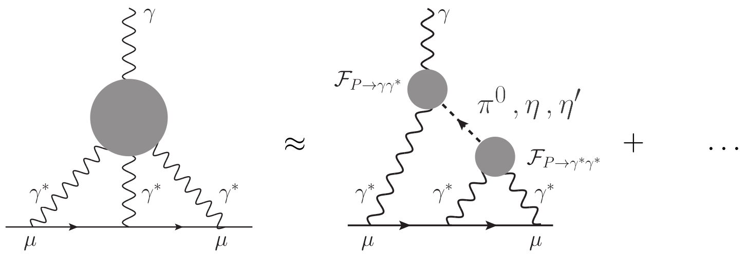
Figure 1: Pseudoscalar pole contribution to hadronic light-by-light scattering in the muon $(g-2)_{\mu}$. Adapted from Ref. [4].

It takes the form

$$a_{\mu}^{P\textrm{-pole}}=\left(\frac{\alpha}{\pi}\right)^{3}\int_{0}^{\infty} dQ_{1}\int_{0}^{\infty}dQ_{2}\int_{-1}^{+1}d\tilde{\tau}$$

$$\bigg{[}w_{1}(Q_{1},Q_{2},\tilde{\tau}){\cal F}_{P\rightarrow\gamma^{*}\gamma^{*}}(-Q_{1}^{2},-(Q_{1}+Q_{2})^{2}){\cal F}_{P\rightarrow\gamma^{*}\gamma^{*}}(-Q_{2}^{2},0)$$

$$+w_{2}(Q_{1},Q_{2},\tilde{\tau}){\cal F}_{P\rightarrow\gamma^{*}\gamma^{*}}(-Q_{1}^{2},-Q_{2}^{2}){\cal F}_{P\rightarrow\gamma^{*}\gamma^{*}}(-(Q_{1}+Q_{2})^{2},0)\bigg{]}\,,$$ (1)

where the nonperturbative information is encapsulated in the transition form factors ${\cal F}_{P\rightarrow\gamma^{*}\gamma^{*}}$ of the pseudoscalar mesons $P=\pi^{0},\eta,\eta^{\prime}$ to two virtual photons. The evaluation of the integrands in Eq. (1) requires the knowledge of the transition form factors (TFFs) at space-like momenta, both in the single and double virtual case. It turns out that these TFFs can indeed be obtained from a QCD calculation on a Euclidean lattice. The relevant kinematic region is determined by the positive weight functions $w_{1}$ and $w_{2}$ which depend on the absolute values of the photon momenta, the kinematic variable $\tilde{\tau}=\cos\theta\in[-1,+1]$, with $\theta$ being the angle between the photon momenta, and the mass of the pseudoscalar meson $P$. In these proceedings we focus on the pion-pole contribution for which first lattice results were obtained in [4, 5].

2 The transition form factors on the lattice

In the continuum Minkowski space the TFFs are defined via the matrix element of two electromagnetic currents $j_{\mu}$ and $j_{\nu}$ and the pseudoscalar state $P$ with four-momentum $p$,

$$M_{\mu\nu}(p,q_{1}) =i\int d^{4}x\,e^{iq_{1}x}\left<0\left|T\{j_{\mu}(x)j_{\nu}(0)\}\right|P(p)\right>$$

$$=\varepsilon_{\mu\nu\alpha\beta}q_{1}^{\alpha}q_{2}^{\beta}{\cal F}_{P\rightarrow\gamma^{*}\gamma^{*}}(q_{1}^{2},q_{2}^{2})\,.$$

For virtualities below the threshold for hadron production, the transition form factors can be analytically continued to Euclidean space, cf. Ref. [4], and are therefore accessible on the lattice. The Euclidean matrix element $M_{\mu\nu}^{E}(p,q_{1})$ can be calculated via an integral over the temporal separation $\tau=t_{i}-t_{f}$ of the two currents,

$$M_{\mu\nu}^{E}=\int_{-\infty}^{\infty}d\tau\,e^{\omega_{1}\tau}\tilde{A}_{\mu\nu}(\tau),\quad i^{n_{0}}M_{\mu\nu}^{E}(p,q_{1})=M_{\mu\nu}(p,q_{1}).$$ (2)

Here, $n_{0}$ denotes the number of temporal indices in $M_{\mu\nu}$, $q_{1}$ and $q_{2}$ are the photon virtualities, $p=q_{1}+q_{2}$ is the on-shell pseudoscalar momentum, $\omega_{1}$ is a real-valued free parameter with $q_{1}=(\omega_{1},\vec{q}_{1})$, and

$$\tilde{A}_{\mu\nu}(\tau)=\left<0\left|T\{j_{\mu}(\vec{q}_{1},\tau)j_{\nu}(\vec{p}-\vec{q}_{1},0)\}\right|P(p)\right>\,.$$

On the lattice this function is recovered from the three-point function

$$C_{\mu\nu}(\tau,t_{P})=a^{6}\sum_{\vec{x},\vec{z}}\langle j_{\mu}(\vec{x},t_{i})j_{\nu}(\vec{0},t_{f})P^{\dagger}(\vec{z},t_{0})e^{i\vec{p}\vec{z}}\rangle e^{-i\vec{x}\vec{q}_{1}}\equiv\langle j_{\mu}j_{\nu}P^{\dagger}\rangle\,,$$ (3)

via

$$\tilde{A}_{\mu\nu}(\tau)=\frac{2E_{P}}{Z_{P}}\lim_{t_{P}\to\infty}e^{E_{P}(t_{f}-t_{0})}C_{\mu\nu}(\tau,t_{P})\,,$$ (4)

where $t_{P}=\min(t_{f}-t_{0},t_{i}-t_{0})$ is the minimal temporal separation between the pseudoscalar and the two vector currents. The pseudoscalar meson energy $E_{P}$ and the factors $Z_{P}$ are determined through appropriate pseudoscalar two-point functions. Before integrating over $\tau$, one can contract the Lorentz structure of the matrix elements. The function $\tilde{A}_{\mu\nu}$ with one or more temporal indices vanishes for the pseudocalar at rest, and the spatial components can be written as $\tilde{A}(\tau)=im_{P}^{-1}\varepsilon_{ijk}\frac{\vec{q}_{1}^{i}}{\vec{q}_{1}^{2}}\tilde{A}_{jk}(\tau)$, and analogously for $C(\tau)$.

The amplitude $C_{\mu\nu}$ contains connected, vector current disconnected, pseudoscalar disconnected, and fully disconnected diagrams as illustrated in Figure 2.

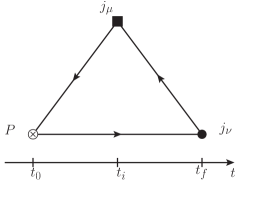
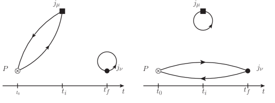
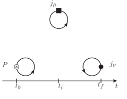
Figure 2: Contributions to the three-point function $C_{\mu\nu}$: Connected (top left), vector current disconnected (top middle and right), pseudoscalar disconnected (bottom left) and fully disconnected (bottom right).

For Wilson fermions the pseudoscalar disconnected diagrams on the second line are zero for $P=\pi_{0}$ by the exact cancellation between the up and down quark loops. For $P=\eta$ and $\eta^{\prime}$ this is not the case and these disconnected diagrams must be included. This is so also for $P=\pi_{0}$ in the twisted mass Wilson fermion discretization, where the diagrams on the second line are nonzero due to the broken isospin symmetry. Since this isospin breaking is a lattice artefact, we consider an isospin rotation $\pi^{0}\rightarrow-i\cdot(\pi^{+}+\pi^{-})$ with a corresponding transformation of the isospin decomposed light quark electromagnetic currents $j^{0,0}_{\mu}\rightarrow j^{0,0}_{\mu}$ and $j^{1,0}_{\mu}\rightarrow i\cdot(j^{1,+}_{\mu}-j^{1,-}_{\mu})$, which allows us to relate the neutral and charged pion form factors. The difference between the two at finite lattice spacing is a lattice artefact of order $O(a^{2})$.

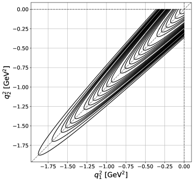
Figure 3: Range of photon virtualities spanned in our calculation on the ensemble cB072.64.

A further simplification is achieved by restricting the considerations to the kinematic situation where the pseudoscalar is at rest, i.e., $\vec{p}=\vec{0}$. Then, the expressions for the photon virtualities simplify to

$$q_{1}^{2}=\omega_{1}^{2}-\vec{q}_{1}^{2}\,,\quad q_{2}^{2}=(m_{P}-\omega_{1})^{2}-\vec{q}_{1}^{2}\,.$$ (5)

As a consequence, for each choice of spatial momentum $\vec{q}_{1}$ one obtains a continuous set of combinations of $q_{1}$ and $q_{2}$ which form an orbit in the $(q_{1}^{2},q_{2}^{2})$-plane as illustrated in Figure 3 for $m_{P}$ set to the physical pion mass. There we show the orbits for all the momenta calculated on the ensemble cB072.64. From Eqs. (5) it becomes clear that the shape of the orbits becomes squeezed along the diagonal as the pseudoscalar mass $m_{P}$ is lowered. This feature makes it particularly challenging to extract single virtual pion transition form factors ${\cal F}_{\pi\rightarrow\gamma^{*}\gamma^{*}}(q_{1}^{2},0)={\cal F}_{\pi\rightarrow\gamma^{*}\gamma^{*}}(0,q_{2}^{2})$ at large momenta $q_{i}^{2}$ on physical point ensembles if one uses only pions at rest. However, the problem can be circumvented by using moving frames, cf. [5]. For $P=\eta$ and $\eta^{\prime}$ the problem is less eminent due to the larger values of the meson masses $m_{P}$.

3 First results at the physical point

After this theoretical discussion we are now in the position to present first results for the transition form factor ${\cal F}_{\pi\rightarrow\gamma^{*}\gamma^{*}}$ of the pion obtained for the ensembles cB072.64 and cC060.80 at the physical point. First, we illustrate the quality of our data with sample results for the amplitude $\tilde{A}(\tau)$ defined in Eq. (4). In Figure 4 we show the full amplitude and separately the fully connected and the vector current disconnected contributions for two of the momentum orbits on the ensemble cB072.64. The vector current disconnected amplitude is multiplied by a factor $-50$ in order to facilitate comparison with the connected contribution and the full amplitude.

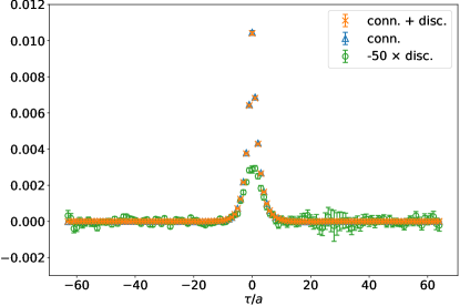
Figure 4: Amplitude $\tilde{A}(\tau)$ for momentum orbit $|\vec{q}^{2}|=10\,(2\pi/L)^{2}$ (left) and $|\vec{q}^{2}|=29\,(2\pi/L)^{2}$ on cB072.64. Shown in orange is the full contribution to $\tilde{A}(\tau)$, in blue the connected contribution and in green the vector current disconnected contribution multiplied by -50.

The examples illustrate that the disconnected contribution is very small, but significant. More generally, we find that in the peak region it is suppressed w.r.t. the connected contribution by a factor between 50 and 200 depending on the orbit. We also conclude from our data that the statistical error on the disconnected contribution is sufficiently well under control on the physical point ensembles.

To obtain the form factor we need to integrate $\tilde{A}(\tau)$ weighted by the factor $\exp(\omega_{1}\tau)$ over the whole temporal axis, cf. Eq. 2. In order to control the statistical error in the exponentially enhanced tail and to be able to integrate up to $\tau\rightarrow\infty$, we proceed as follows. First, we fit the lattice data by a model function $\tilde{A}^{\textrm{(fit)}}(\tau)$ in a range $\tau_{\textrm{min}}\leq|\tau|\leq\tau_{\textrm{max}}$, and then we replace the lattice data $\tilde{A}^{\textrm{(latt.)}}(\tau)$ by the data from the fit for $\tau>\tau_{\textrm{cut}}$,

$${\cal F}_{\pi\rightarrow\gamma^{*}\gamma^{*}}(q_{1}^{2},q_{2}^{2})=\int_{-\infty}^{\tau_{\textrm{cut}}}d\tau\,\tilde{A}^{\textrm{(latt.)}}(\tau)e^{\omega_{1}\tau}+\int_{\tau_{\textrm{cut}}}^{\infty}d\tau\,\tilde{A}^{\textrm{(fit)}}(\tau)e^{\omega_{1}\tau}.$$ (6)

Following Ref. [4] we use both a vector meson dominance (VMD) model and the lowest meson dominance (LMD) model to estimate the model dependence. We perform global fully correlated fits, i.e., we simultaneously fit all momentum orbits in the range $\tau_{\textrm{min}}\leq|\tau|\leq\tau_{\textrm{max}}$ and take into account the correlation between all fitted data. In Figure 5

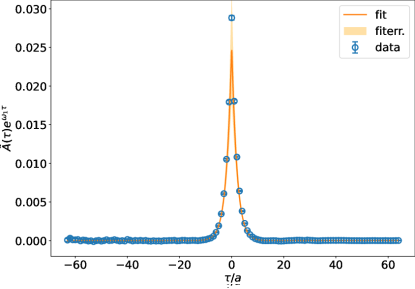
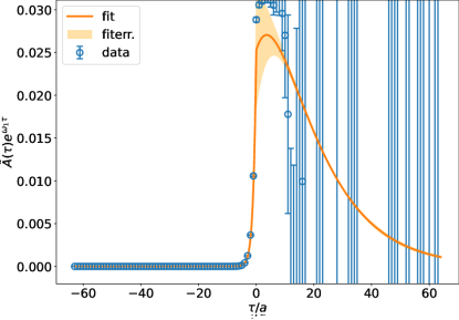
Figure 5: Integrand $\tilde{A}(\tau)e^{\omega_{1}\tau}$ on cB072.64 with LMD model fits for momentum orbit $|\vec{q}^{2}|=2\,(2\pi/L)^{2}$. Diagonal kinematics with $a\omega_{1}=am_{\pi}/2\approx 0.0284$ (left), single virtual kinematics with $a\omega_{1}=a|\vec{q_{1}}|\approx 0.1388$ (right).

we illustrate the procedure by showing the result for the integrand $\tilde{A}(\tau)e^{\omega_{1}\tau}$ of a typical global fit to $\tilde{A}(\tau)$ in the range $9\leq|\tau/a|\leq 12$ with $\chi^{2}/\textrm{dof}=1.20$ on the ensemble cB072.64 using the LMD model. The plot on the left shows the resulting integrand for the diagonal kinematics $q_{1}^{2}=q_{2}^{2}$, while the plot on the right shows it for the single virtual kinematics with $q_{1}^{2}=0$. The transition form factors obtained from the integration over the lattice data and the fitted data depend of course on the choice of the model, the fit range and the value $\tau_{\textrm{cut}}$. The variations resulting from these choices are carried through all further analysis steps and are included in the systematic error estimate of the final result for $a_{\mu}$. The typical values of $\tau_{\textrm{cut}}$ we use in our analysis result in a data content of well above 98% for most of the TFFs. However, for TFFs with (close to) single virtual kinematics, the data content is sometimes also less for higher momentum orbits. Here, the data content is defined as the fraction of the TFF coming from the first term in Eq. (6).

Once the form factors are obtained in the whole kinematic region as described by the yield plot in Figure 3, we parameterize them using a modified $z$-expansion of the form

$$P(Q_{1}^{2},Q_{2}^{2})\cdot\mathcal{F}_{\pi\gamma^{*}\gamma^{*}}(-Q_{1}^{2},-Q_{2}^{2})=\\ \sum_{m,n=0}^{N}c_{nm}\left(z_{1}^{n}-(-1)^{N+n+1}\frac{n}{N+1}z_{1}^{N+1}\right)\left(z_{2}^{m}-(-1)^{N+m+1}\frac{m}{N+1}z_{2}^{N+1}\right)$$ (7)

where $z_{k}=z(Q_{k}^{2})$ are modified four-momenta and $P(Q_{1}^{2},Q_{2}^{2})$ is a polynomial, see Ref. [5] and references therein for further details. We determine the coefficients $c_{nm}$ by fitting Eq. (7) to samples of ${\cal F}_{\pi\rightarrow\gamma^{*}\gamma^{*}}(-Q_{1}^{2},-Q_{2}^{2})$ in the $(Q_{1}^{2},Q_{2}^{2})$-plane. The sample points are given by a set of fixed values of $Q_{2}^{2}/Q_{1}^{2}$ on all momentum orbits, and we ensure that all included data points pass a certain threshold for the data content. In Figure 6 we show the result of such a (fully correlated) fit with $\chi^{2}/\textrm{dof}=0.96$ using $Q_{2}^{2}/Q_{1}^{2}=1.0,0.59,0.0$, and $N=2$ to the TFFs obtained from a global LMD fit with $\{\tau_{\textrm{min}}/a,\tau_{\textrm{max}}/a\}=\{9,12\}$, $\chi^{2}/\textrm{dof}$ = 1.20, $\tau_{\textrm{cut}}/a$ = 20 and a threshold of 90% on the ensemble cB072.64.

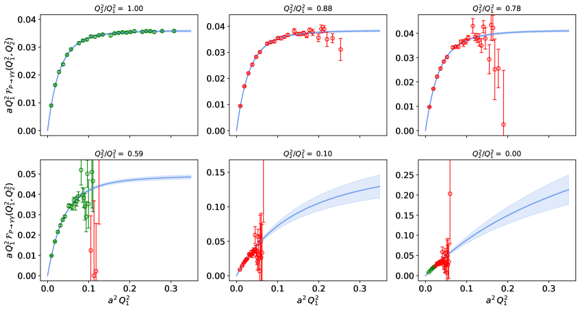
Figure 6: Illustration of transition form factors and their parameterization using the fitted modified $z$-expansion. Only the data coloured in green is included in the fit.

As a crosscheck for the quality of the fit we also show the data for three other ratios $Q_{2}^{2}/Q_{1}^{2}=0.88,$ 0.78, and 0.10 not included in the fit together with the fitted modified $z$-expansion. The variations resulting from varying the sampling of ${\cal F}_{\pi\rightarrow\gamma^{*}\gamma^{*}}(-Q_{1}^{2},-Q_{2}^{2})$ in the momentum plane are also included in the systematic error estimate of the final result for $a_{\mu}$.

Finally, having the parameterization of the TFFs at hand, we can use it in the three-dimensional integral representation in Eq. (1) and calculate the bare pion-pole contribution $a_{\mu}^{\pi\textrm{-pole, bare}}$ to the anomalous magnetic moment. In Figure 7 we show the results for $a_{\mu}^{\pi\textrm{-pole, bare}}$ on the two ensembles at the physical point as a function of $\tau_{\textrm{cut}}/a$. Each data point is a weighted average of $O(100)$ results from different fits for $\tilde{A}$ using VMD or LMD with different fit ranges and different fits using the modified $z$-expansion on different samplings in the momentum plane. The weighted average is obtained using weights inspired by the Akaike information criterion (AIC). The error therefore includes the variation w.r.t. the fitting of $\tilde{A}$ and the sampling of ${\cal F}_{\pi\rightarrow\gamma^{*}\gamma^{*}}$ in the $(Q_{1}^{2},Q_{2}^{2})$-plane.

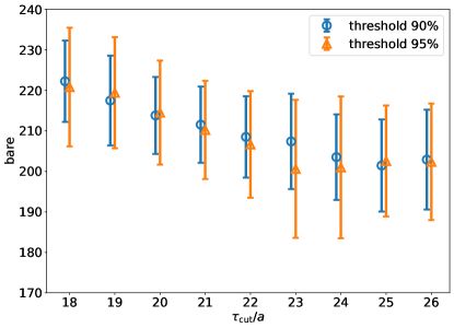
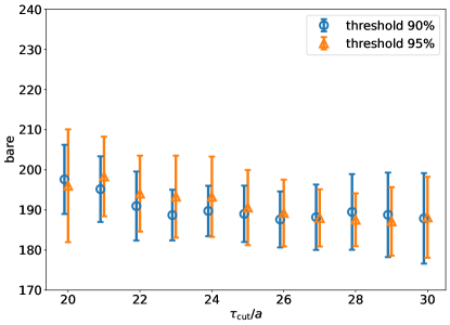
Figure 7: AIC averaged data for a range of $\tau_{\textrm{cut}}/a$ for the ensembles cB072.64 (left) and cC060.80 (right).

The variation of the final result with $\tau_{\textrm{cut}}$ indicates a residual dependence on the specific procedure of variance reduction in the large-$\tau$ tail of $\tilde{A}$. In principle, this dependence is removed in the limit $\tau_{\textrm{cut}}\rightarrow\infty$, but if $\tau_{\textrm{cut}}$ is chosen too large the $z$-expansion fits become unstable and hence the final result unreliable. Our results in Figure 7 indicate that choosing $\tau_{\textrm{cut}}\in[1.8,2.1]$ fm seems a safe choice and we perform a further AIC averaging over this range. This yields the bare results shown in Table 2 for the two physical point ensembles, with total errors in the 5%-8% range.

$a_{\mu}^{\pi-\text{pole, bare}}\cdot 10^{-11}$	threshold 90%	threshold 95%
cB072.64	208.9(10.1)(7.8)[12.8]	204.5(14.2)(6.3)[15.6]
cC060.80	188.9(9.9)(2.7)[10.2]	187.9(9.0)(1.9)[9.2]

Table 2: Bare results using the AIC procedure on the two physical point ensembles. The first error is the statistical error, the second the systematic error and the third the total error.

Since we use local iso-vector and iso-vector axial current operators in our amplitude $C_{\mu\nu}$, instead of conserved (point-split) current operators, we need to renormalize the bare results by the corresponding renormalization constants. Preliminary values are available for our setup from a calculation within ETMC.

4 Conclusion and outlook

After applying the renormalization factors and performing a rough estimate of the continuum limit, we obtain a preliminary value $a_{\mu}^{\pi-\text{pole}}=53.7(2.6)(3.1)[4.0]\cdot 10^{-11}$. This can be compared to the recent lattice result $a_{\mu}^{\pi-\text{pole}}=59.7(3.6)\cdot 10^{-11}$ from Ref. [5] and the dispersive result $a_{\mu}^{\pi-\text{pole}}=63.0^{+2.7}_{-2.1}\cdot 10^{-11}$ from Refs. [6, 7, 8], and we find agreement within 1 to 2 standard deviations. Finalizing the analysis might result in a slightly different central value, however, we expect that the relative total error will stay below the 10% level. We plan to analyze a third physical point ensemble at a finer lattice spacing which will result in a more robust continuum limit extrapolation. We also plan to calculate the form factors for the pion in a moving frame and to perform the analysis of the $\eta$- and $\eta^{\prime}$-pole contributions, and to include ensembles with larger pion masses.

References

- [1] Extended Twisted Mass collaboration, C. Alexandrou et al., Quark masses using twisted-mass fermion gauge ensembles, Phys. Rev. D 104 (2021) 074515, [2104.13408].
- [2] Extended Twisted Mass collaboration, C. Alexandrou et al., Ratio of kaon and pion leptonic decay constants with Nf=2+1+1 Wilson-clover twisted-mass fermions, Phys. Rev. D 104 (2021) 074520, [2104.06747].
- [3] M. Knecht and A. Nyffeler, Hadronic light by light corrections to the muon g-2: The Pion pole contribution, Phys. Rev. D 65 (2002) 073034, [hep-ph/0111058].
- [4] A. Gérardin, H. B. Meyer and A. Nyffeler, Lattice calculation of the pion transition form factor , Phys. Rev. D 94 (2016) 074507, [1607.08174].
- [5] A. Gérardin, H. B. Meyer and A. Nyffeler, Lattice calculation of the pion transition form factor with Wilson quarks, Phys. Rev. D 100 (2019) 034520, [1903.09471].
- [6] T. Aoyama et al., The anomalous magnetic moment of the muon in the Standard Model, Phys. Rept. 887 (2020) 1–166, [2006.04822].
- [7] M. Hoferichter, B.-L. Hoid, B. Kubis, S. Leupold and S. P. Schneider, Pion-pole contribution to hadronic light-by-light scattering in the anomalous magnetic moment of the muon, Phys. Rev. Lett. 121 (2018) 112002, [1805.01471].
- [8] M. Hoferichter, B.-L. Hoid, B. Kubis, S. Leupold and S. P. Schneider, Dispersion relation for hadronic light-by-light scattering: pion pole, JHEP 10 (2018) 141, [1808.04823].