Quantum readout error mitigation via deep learning

Abstract

Quantum computing devices are inevitably subject to errors. To leverage quantum technologies for computational benefits in practical applications, quantum algorithms and protocols must be implemented reliably under noise and imperfections. Since noise and imperfections limit the size of quantum circuits that can be realized on a quantum device, developing quantum error mitigation techniques that do not require extra qubits and gates is of critical importance. In this work, we present a deep learning-based protocol for reducing readout errors on quantum hardware. Our technique is based on training an artificial neural network with the measurement results obtained from experiments with simple quantum circuits consisting of singe-qubit gates only. With the neural network and deep learning, non-linear noise can be corrected, which is not possible with the existing linear inversion methods. The advantage of our method against the existing methods is demonstrated through quantum readout error mitigation experiments performed on IBM five-qubit quantum devices.

I Introduction

The theory of quantum computation opens up tremendous opportunities as it promises drastic computational benefits for solving commercially relevant problems [1, 2, 3, 4, 5]. One of the major technological hurdles against practical quantum advantage is the unavoidable noise and imperfections. Although the theory of quantum error correction and fault-tolerance guarantees that imperfections are not the fundamental objections to quantum computation  [6, 7, 8, 9, 10], the size of quantum circuits needed to realize the theory is beyond the reach of the near-term technology. Consequently, in near-term quantum computing, all physical qubits are expected to be operating as logical qubits, leading to the Noisy Intermediate-Scale Quantum (NISQ) era [5]. Therefore, to bridge the gap between theoretical results and experimental capabilities, developing algorithmic means at the software level to reduce quantum computational errors without increasing the quantum resource overhead, such as the number of qubits and gates, is desired [11, 12, 13, 14, 15].

This work addresses the problem of reducing the readout errors that occur during the final step of the quantum computation. We propose a machine learning-based protocol to reduce the quantum readout error. Our method trains an artificial neural network with real measurement outcomes from quantum circuits with known final states as input and ideal measurement outcomes of the same circuit as output. After training, the neural network is used to infer the ideal measurement outcomes from real measurement outcomes of arbitrary quantum computation. Since our quantum readout error mitigation (QREM) protocol only relies on training a classical neural network with known measurement outcomes, the extra quantum resource arises only for gathering noisy measurement results. This is done with a random state prepared by applying an arbitrary single-qubit gate to the default initial state of qubits that are subject to measurement in a quantum algorithm. Thus our method does not increase the number of qubits and gates beyond what is needed by the quantum algorithm itself.

Using the neural network and deep learning, non-linear readout errors can be corrected. This feature places our QREM method above the predominantly used methods based on linear inversion that do not take non-linear effects into account. Moreover, while the linear inversion method often produces non-physical results and requires post-optimization, our method always produces physically valid results. We compare our QREM with the linear inversion method through experiments with superconducting quantum devices available on the IBM cloud platform for two to five qubits. The experimental results demonstrate that the amount of readout error reduced by our method exceeds that of the previous method in all instances differentiated by the number of qubits and the error quantifier selected from mean squared error, Kullback-Leibler divergence and infidelity.

The remainder of the paper is organized as follows. Section II describes the theoretical framework of this work, such as the quantum readout error, existing mitigation methods for it, and the underlying idea of our neural network-based approach to the problem. Section III explains the machine learning algorithm used in this work for the quantum readout error mitigation. Section IV.1 presents the proof-of-principle experiment performed with three five-qubit quantum computers available on the IBM Quantum cloud platform. Conclusions and directions for future work are provided in Sec. V.

II Theoretical Framework

Quantum computation can be thought of as a three-step procedure consisting of input state initialization, unitary transformation, and readout. In experiments, the readout step is usually implemented as the projective measurement in the computational basis, which collapses an $n$-qubit final state $|\psi_{j}\rangle\in\mathbb{C}^{2^{n}}$ to $|i\rangle$ with the probability $p(i|j)=|\innerproduct{i}{\psi_{j}}|^{2}$. Without loss of generality, we denote $p(i)\coloneqq p(i|j)$. In the ideal (error free) case, the final result of a quantum algorithm is determined by the probability distribution of the measurement outcomes, denoted by

$$\bm{p}=\{p(0),p(1),\ldots,p(2^{n}-1)\}.$$

Equivalently, $\bm{p}$ is the set of diagonal elements of the final density matrix $\rho$ produced at the end of the quantum computation. Many quantum algorithms are designed in a way that the solution to the problem is encoded in the probability distribution $\bm{p}$. In particular, estimating an expectation value of some observable from such probability distribution is central to many NISQ algorithms, such as Variational Quantum Eigensolver (VQE) [16, 17, 18, 19], Quantum Approximate Optimizatoin Algorithm (QAOA) [20], Quantum Machine Learning (QML) [21, 22, 23], and simulation of stochastic processes [24, 25].

However, due to readout errors, the observed probability distribution can deviate from the ideal probability distribution. Hereinafter, we denote the probability to observe $|i\rangle$ in the experiment as $\hat{p}(i)$ and the error map as $\mathcal{N}$ that transforms the ideal probability vector to an observed one as $\hat{\bm{p}}=\mathcal{N}(\bm{p})$. Since $\mathcal{N}$ describes the transformation of a probability distribution, it must preserve the 1-norm. The goal of QREM is to minimize the loss function

$$D\left(\bm{p},\mathcal{N}(\bm{p})\right),$$ (1)

defined by some distance measure $D$ for probability distributions. The goal of QREM is conceptually depicted at the top of Fig. 1, with an example of a two-qubit case given in the bottom.

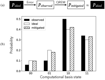
Figure 1: An illustration of the quantum readout error mitigation (QREM) procedure. In the noiseless case, the underlying quantum algorithm should generate a probability distribution $\boldsymbol{p}_{ideal}$ upon the measurement in the computational basis. However, due to imperfections and noise, one obtains the noisy distribution $\boldsymbol{p}_{observed}$, which deviates from the true distribution. The QREM method constructs a probability distribution $\boldsymbol{p}_{mitigated}$ based on $\boldsymbol{p}_{observed}$ that is as close to $\boldsymbol{p}_{ideal}$ as possible. The bar graph in (b) is an artificially generated two-qubit example that illustrates the role of QREM. After a QREM algorithm, $\boldsymbol{p}_{mitigated}$ is a more accurate description of the true probability distribution than the raw data.

Since QREM is of critical importance especially for NISQ computing, several protocols have been proposed recently to address this issue. In essence, these methods assume that the noisy function is linear and relies on solving the linear equation

$$\hat{\bm{p}}=\Lambda\bm{p},$$ (2)

where the linear response matrix $\Lambda$ is estimated by some tomographic means [18, 26, 27, 28, 29, 30, 31, 32]. This usually demands $O(2^{n})$ measurements with an assumption that the computational basis state preparation error is negligible compared to the readout error. The number of experiments can be reduced with certain assumptions about the noise model, such as those dominated by few-qubit correlations [33, 30, 31] and by independent single-qubit Pauli errors acting on the final state during the finite time between the last gate and the detection event [34]. After $\Lambda$ is found, correct measurement outcomes are predicted by calculating $\Lambda^{-1}\hat{\bm{p}}$. We refer to this technique as linear inversion (LI) based QREM (LI-QREM). This approach often requires extra classical post-processing [28, 29, 31], since the inversion may produce a vector that is not a probability distribution. In general, the readout noise is not static. Hence the QREM procedure described above needs to be frequently implemented as a part of the calibration routine of the given experimental setup.

While this work shares the same goal as the previous methods, we leverage classical deep learning techniques to approximate $\mathcal{N}^{-1}(\bm{p})$. Namely, we train a neural network (NN) denoted by $\mathcal{F}$ which describes the map $\bm{p}=\mathcal{F}(\hat{\bm{p}})$ such that $\mathcal{F}\approx\mathcal{N}^{-1}$. Since the deep learning model can take care of spurious non-linear effects, the amount of error suppression is expected to be beyond what the linear model can achieve. Moreover, by using the softmax function in the final layer of a neural network, one can ensure that the output always represents a probability distribution. Figure 2 compares the basic idea of previous LI-QREM and the neural network based method proposed in this work, which we refer to as NN-QREM.

Figure 2: QREM based on (a) linear error model and readout tomography (LI-QREM) (b) deep learning (NN-QREM). The deep learning model is trained to implement the function $\mathcal{F}$, which serves as an approximation to the inverse of the true error map, i.e. $\mathcal{F}\approx\mathcal{N}^{-1}$.

The following section explains the machine learning model in detail.

III The Machine Learning Algorithm

III.1 Data collection for training

In order to train a deep neural network for QREM, we need to have both $\bm{p}$ and $\hat{\bm{p}}$, meaning that qubits need to be prepared in some known state before measurement. Since single-qubit gate errors are usually negligible when compared to those of two-qubit gates and measurement in modern quantum devices [27, 28, 35], we prepare the training set of quantum states using single-qubit gates only. In particular, the training set is constructed by applying $R_{y}(\theta)$ gate, which corresponds to the rotation around the y-axis of the Bloch sphere, to all qubits in the system with randomly and independently generated angle $\theta\in[0,2\pi)$. Since the measurement is performed in the computational basis, which is the $\sigma_{z}$ basis by convention, there is no need to apply the $R_{z}$ gate. Hence the quantum circuit depth for generating a training data is one. Figure 3 represents the quantum circuit that generates $\hat{\bm{p}}$ as an input to the neural network for training. The ideal probability distribution $\bm{p}$, which is inserted as the output of the neural network during training, can easily be calculated from the rotation angles. For an $n$-qubit system, the probability to measure a computational basis state $b\in\{0,1\}^{n}$ (i.e. an $n$-bit string) is

$$p(b)=\left|\prod_{i}^{n}\cos^{1-b_{i}}(\theta_{i}/2)\sin^{b_{i}}(\theta_{i}/2)\right|^{2},$$

where $b_{i}$ is the $i$th bit of the binary string $b$.

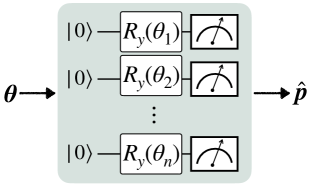
Figure 3: The quantum circuit for generating the noisy probability distribution $\hat{\bm{p}}$ used as an input to the neural network during training. The training data is generated by applying an arbitrary single-qubit rotation $R_{y}(\theta)$ to each qubit and measuring qubits in the computational basis. Training of the neural network also requires the ideal probability distribution $\bm{p}$, and this is calculated using the set of rotation angles $\bm{\theta}$ used in the quantum circuit.

III.2 Model construction

The deep learning model is constructed with an input layer, hidden layers, and an output layer (see Fig. 2 (b)). Input layer and output layer have $2^{n}$ nodes, whose numerical values represent the probability of measuring the computational basis states in the actual experiment and the ideal case, respectively. All hidden layers are fully connected layers, and each hidden node employs the Rectified Linear Unit (ReLU) as the activation function. The output layer uses the softmax function for activation, which ensures that the output represents a probability distribution. The loss function for optimizing the weights and biases of the neural network is the categorical cross entropy, which is normally used in multi-label classification problems. The free parameters are updated by the Adam optimizer [36] whose hyperparameters, such as the learning rate, are empirically chosen (see Sec. IV.1).

III.3 Inference

The trained neural network represents the function $\mathcal{F}\approx\mathcal{N}^{-1}$. Thus, the error-mitigated probability distribution, which is denoted by $\tilde{\bm{p}}$, is obtained by inserting $\hat{\bm{p}}$ from an experiment of interest as the input to the trained neural network. The inference can be expressed as $\tilde{\bm{p}}=\mathcal{F}(\hat{\bm{p}})\approx\mathcal{N}^{-1}(\hat{\bm{p}})$.

IV Experiment

IV.1 Experimental Setup

Two quantum readout error mitigation techniques, namely LI-QREM and NN-QREM were tested on three different five-qubit quantum computers available on IBM Quantum Experience. Training of the neural network and inference are carried out as described in Sec. III using Keras library of Python. The LI-QREM results are obtained by using the default readout error mitigation package in Qiskit Ignis [37] (i.e. $\mathtt{CompleteMeasFitter}$). We use the least squares method to calibrate the resulting matrix from the Qiskit library to ensure physical results.

On the five-qubit devices, QREM of two to five qubits are carried out. The quantum devices with smaller quantum volume were chosen in this study since the error mitigation is more critical for such devices. Furthermore, we chose devices of different qubit connectivity as shown in Fig. 4. For the first arrangement (Fig. 4 (a)), two quantum devices were selected based on the amount of queue on the cloud service, namely ibmq_quito and ibmq_belem, to minimize the experimental time. The two- and three-qubit QREM were performed on ibmq_quito, and the four- and five-qubit QREM experiments were performed on ibmq_belem. For the second arrangement, ibmq_qx2 was the only device available for us to use. Thus for this device, all two- to five-qubit experiments were implemented.

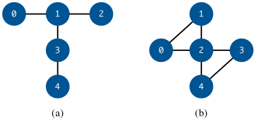
Figure 4: Coupling map (qubit connectivity) of the quantum devices used in this work. ibmq_quito and ibmq_belem have the arrangement shown in (a), and ibmq_qx2 has the arrangement shown in (b).

Several hyperparameters need to be fixed when training a neural network. In our experiments, we set the number of nodes in each hidden layer to be $5\times 2^{n}$ to ensure that the number of nodes scales only linearly with the size of the probability distribution. The learning rate for the Adam optimization algorithm was fine-tuned for each number of qubits. The number of hidden layers was optimized using 5-fold cross-validation (see Supplementary Information). The hyperparameter values of the neural networks used in the NN-QREM experiments are provided in Tab. 1 and Tab. 2 for the two device types shown in Fig. 4, respectively.

Num. of qubits	2	3	4	5
Num. of training data	1175	3472	9700	9700
Num. of test data	200	200	200	200
Num. of hidden layer	7	4	8	5
Num. of nodes in each hidden layer	20	40	80	160
Num. of epochs	300	300	300	300
Learning rate	0.001	0.001	$5\times 10^{-5}$	$5\times 10^{-5}$

Table 1: The hyperparameters and training details of the neural networks used in the NN-QREM experiments with two to five qubit in case of ibmq_belem and ibmq_quito.

Num. of qubits	2	3	4	5
Num. of training data	1800	3800	7800	9850
Num. of test data	200	200	200	200
Num. of hidden layer	5	2	7	5
Num. of nodes in each hidden layer	20	40	80	160
Num. of epochs	300	300	300	300
Learning rate	0.001	0.001	$5\times 10^{-5}$	$5\times 10^{-5}$

Table 2: The hyperparameters and training details of the neural networks used in the NN-QREM experiments with two to five qubit in case of ibmq_qx2.

IV.2 Loss functions

In this work, we evaluate three different distance measures (see Eq. (1)) to quantify the amount of readout error mitigation and to compare the performance of different QREM methods. The metrics used for comparison are mean squared error (MSE)

$$D_{\mathrm{MSE}}=\dfrac{1}{2^{n}}\sum\limits_{i=0}^{2^{n}-1}{|\bm{\tilde{p}}_{i}-\bm{p}_{i}|^{2}},$$

Kullback-Leibler divergence (KLD)

$$D_{\mathrm{KLD}}=\sum\limits_{i=0}^{2^{n}-1}{\bm{p_{i}}\log{\dfrac{\bm{p}_{i}}{\bm{\tilde{p}}_{i}}}},$$

and infidelity (IF)

$$D_{\mathrm{IF}}=1-\left(\sum\limits_{i=0}^{2^{n}-1}{\sqrt{\bm{p}_{i}\bm{\tilde{p}}_{i}}}\right)^{2},$$

where $\bm{p}_{i}$ and $\bm{\tilde{p}}_{i}$ are the $i$th elements of the ideal and the mitigated probability distributions, respectively. For all these measures, a smaller value indicates a better performance as they represent the dissimilarity. Moreover, the infidelity is equivalent to the quantum state infidelity of two diagonal density matrices.

IV.3 Results

Figure 5: Experimental QREM results for reducing (a) MSE, (b) KLD and (c) infidelity from ibmq_quito and ibmq_belem. Filled bars represent unmitigated results, unfilled bars represent the LI-QREM results, and the hatched bars represent NN-QREM results.

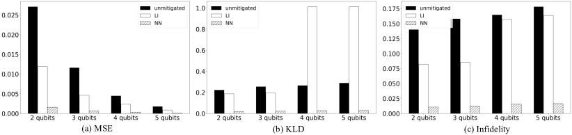
Figure 6: Experimental QREM results for reducing (a) MSE, (b) KLD and (c) infidelity from ibmq_qx2. Filled bars represent unmitigated results, unfilled bars represent the LI-QREM results, and the hatched bars represent NN-QREM results.

This section reports MSE, KLD and IF of (1) the raw (noisy) probability distribution $\bm{\hat{p}}$ (2) LI-QREM results $\bm{\tilde{p}}_{\mathrm{LI}}$ and (3) NN-QREM results $\bm{\tilde{p}}_{\mathrm{NN}}$ that are averaged over 200 test data. The QREM results are presented in Fig. 5 and Fig. 6 for the device type (a) and (b), respectively. The results clearly show that the NN-QREM can reduce the readout noise more effectively than the LI-QREM. Interestingly, LI-QREM is unable to reduce KLD in some cases, while NN-QREM reduces all quantifiers of the error in all cases.

To quantitatively compare the two methods, we define the performance improvement ratio for each loss function $D_{i}$ with the subscript $i$ being MSE, KLD, or IF, as

$$R_{i}=\frac{D_{i}^{\mathrm{LI}}-D_{i}^{\mathrm{NN}}}{D_{i}^{\mathrm{NN}}}\times 100(\%),$$ (3)

where the superscript indicates whether the result is from LI-QREM or NN-QREM. By the definition of $R_{i}$, $R_{i}>0$ indicates that NN-QREM is better than LI-QREM, and vice versa. Table 3 shows the performance improvement ratio for all metrics. The values in the table show that NN-QREM outperforms LI-QREM in all instances. A notable observation is that NN-QREM works particularly better for the device type (b). We speculate that the readout noise in device (b) has higher non-linearities than that of device (a), albeit rigorous device-dependence analysis is left our for future work.

	Num. of qubits	2	3	4	5
Device Type (a)	$R_{\mathrm{MSE}}$	19.9	18.4	30.4	17.6
	$R_{\mathrm{KLD}}$	174	466	59.8	200
	$R_{\mathrm{IF}}$	52.5	76.6	51.2	57.2
Device Type (b)	$R_{\mathrm{MSE}}$	648	564	611	592
	$R_{\mathrm{KLD}}$	888	775	3469	3305
	$R_{\mathrm{IF}}$	657	571	892	890

Table 3: Performance improvement ratio $R_{i}$ for all metrics tested in this work (i.e. MSE, KLD and IF) for each number of qubits. These numbers are categorized under two different device structures shown in Fig. 4, labeled as Type (a) and Type (b)

While the main purpose of our experiment is to demonstrate that the NN-based method is capable of mitigating the readout error beyond the existing linear inversion based methods, we point out that the neural networks used in this work can be further improved. For instance, one can choose to optimize the number of nodes in each hidden layer, instead of using some fixed number. One may also choose to use different activation functions and a different optimization algorithm, such as the Nesterov moment optimizer [38]. One may also explore various loss functions for optimization. For example, one can choose the MSE, KLD or IF as the loss function to minimize through training, instead of the cross entropy loss used in this work.

Another interesting question is whether the neural network trained based on the data generated from one quantum device can be used to mitigate the noise of other quantum devices. This method is expected to work well especially for devices with the similar hardware characteristics. We tested this idea on ibmq_quito and ibmq_belem, since they have similar hardware design with the same qubit connectivity. In particular, we applied the neural network trained with the two- and three-qubit datasets generated by ibmq_quito to mitigate the readout error in the dataset of ibmq_belem. The corresponding QREM results are presented in Tab. 4. The experimental results show that the NN-QREM is better than the LI-QREM for all instances, except for reducing MSE in the case of three-qubit readout error.

	Num. of qubits	2	3
ibmq_quito to ibmq_belem	$R_{\mathrm{MSE}}$	6.55	-10.8
	$R_{\mathrm{KLD}}$	379	470
	$R_{\mathrm{IF}}$	82.5	71.4

Table 4: Performance improvement ratio $R_{i}$ for three metrics (i.e. MSE, KLD and IF) for mitigating the readout error of ibmq_belem using the datasets acquired from ibmq_quito.

V Conclusion

This work proposes quantum readout error mitigation protocol based on deep learning with neural networks. The deep learning is known to be useful for finding non-linear relationships in a given dataset. This feature is utilized in our work to mitigate non-linear effects in the readout error. Hence our approach can achieve the level of error mitigation that is not attainable with the previous methods that rely on the linear error model. The advantage was clearly demonstrated through proof-of-principle experiments with two to five superconducting qubits. In all instances of experiments performed in this work, the neural network based QREM (NN-QREM) outperformed the linear inversion based QREM (LI-QREM) in reducing the error, which is quantified with three different measures: mean squared error, Kullback-Leibler divergence and infidelity. The improvement in error suppression is particularly more significant when Kullback-Leibler divergence and infidelity are considered. We also tested whether the data collected from one quantum device can be used to mitigate the readout error of the other devices. For example, we performed NN-QREM and LI-QREM to mitigate the readout error of ibmq_belem using the data obtained from ibmq_quito. Both methods can successfully mitigate the readout error when MSE and infidelity are considered, while only NN-QREM can also reduce KLD. Moreover, NN-QREM performed better than LI-QREM for this task in all instances, except in the case of three-qubits experiment with MSE.

Some remaining open problems and directions for future work are provided as follows. An important challenge in the domain of quantum error mitigation is the scalability of the algorithm, i.e. the total computational cost should not grow superpolynomially with the number of qubits. In our current construction, even if the number of training data is restricted to grow as $O(poly(n))$, the number of input and output nodes is $2^{n}$. However, the probability vector constructed by sampling from a quantum circuit is sparse as long as the number of repetition does not grow exponentially with $n$. Based on this observation, we plan to investigate machine learning methods for sparse data to explore the possibility of designing a scalable QREM algorithm. Another interesting future work is to develop a machine learning-based QREM protocol for the single-shot settings, which is important for many applications such as quantum teleportation, quantum error correction, and quantum communication.

Supplementary Information: Quantum readout error mitigation via deep learning

I Optimization of the number of hidden layers

This section explains the optimization procedure to decide the number of hidden layers of the neural network. In order to find the optimal number of hidden layers, $k$-fold cross-validation is carried out while changing the number of layers. The $k$-fold cross-validation process is summarized as follows:

1. Set the neural network model and its hyperparameters.

2. Split training data into $k$ sets of the same size.

3. Select one set as a validation set, and the other sets as a training set.

4. Train the neural network with the training set and calculate the score of the model through testing with the validation set.

5. Iterate through steps 3 to 4 $k$ times and calculate the average score of the model.

6. Iterate through steps 1 to 5 and select the model with the best average score.

The work presented in the main manuscript selects $k$ to be 5 and uses infidelity (IF) as the score. After the process, the model with the smallest average infidelity is selected for QREM experiments. The 5-fold cross-validation method is depicted in Supplementary Fig. 1.

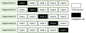
SUPPLEMENTARY FIG. 1: For 5-fold cross-validation, training set is divided into 5 subsets. The validation set is changed for each experiment and other sets that are not selected as the validation set remain as the training set. The black box indicates a validation set for the experiment. The white box indicates the training set for the experiment.

The average infidelity score as a function of the number of layers obtained during the 5-fold cross-validation process is shown in Supplementary Fig. 2 for quantum devices of type (a) and (b) (see Fig. 4 of the main manuscript for the device types).

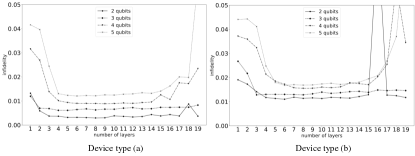
SUPPLEMENTARY FIG. 2: The average infidelity as a function of the number of layers for the quantum device of type (a) and for the device of type (b). The number of qubits used in both device types ranges from two to five.

II Robustness of QREM methods against drift

In general, the readout noise is not static. Hence QREM procedures described in the main manuscript needs to be carried out frequently as a part of the experimental calibration routine. Since QREM procedures can be costly, it is desirable to design QREM to be robust to the drift.

In the following, we show that the neural network-based QREM (NN-QREM) is more robust to the drift than the linear inversion-based QREM (LI-QREM). Recall that in the main manuscript the performance improvement ratio for each loss function $D_{i}$ with the subscript $i$ being MSE, KLD, or IF, is defined as

$$R_{i}=\frac{D_{i}^{\mathrm{LI}}-D_{i}^{\mathrm{NN}}}{D_{i}^{\mathrm{NN}}}\times 100(\%),$$ (S1)

where the superscript indicates whether the result is from LI-QREM or NN-QREM. By the definition of $R_{i}$, $R_{i}>0$ indicates that NN-QREM is better than LI-QREM, and vice versa. Supplementary Figure 3 shows the performance improvement ratio obtained with $\mathtt{ibmq\_belem}$ for 5-qubit QREM from 2021-06-25 to 2021-07-05 while the pre-trained neural network and the linear error matrix are fixed. The figure shows the mean values of 200 test data and the gray shaded region is the standard error. The training data for the neural network are collected from 2021-06-02 to 2021-06-11, and the data for the linear error matrix tomography are collected on 2021-06-17.

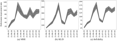
SUPPLEMENTARY FIG. 3: The performance improvement ratio of (a) MSE, (b) KLD, and (c) IF obtained from 2021-06-25 to 2021-07-05 while the pre-trained neural network and the linear error matrix are fixed. The figure shows the mean values of 200 test data and the gray shaded region is the standard error. The training data for the neural network are collected from 2021-06-02 to 2021-06-11, and the data for the error matrix tomography are collected on 2021-06-17.

For all loss functions, $R_{i}$ is greater than zero at all times and it qualitatively increases over time, indicating that the NN-QREM is more robust to drift than LI-QREM.

III Training with smaller dataset

The time required for training the neural network can be reduced by using a fewer number of training data. We tested the NN-QREM method with a smaller training dataset to see whether the good error mitigation performance can be retained while reducing the time cost. All hyperparameters and the test data are the same as the main paper, except the number of the training data is reduced by half. Despite having a smaller dataset, NN-QREM still performs better than LI-QREM as shown in SUPPLEMENTARY FIG.  4 and SUPPLEMENTARY TABLE  1. However, when two NN-QREM protocols with a different amount of training data are compared, the one with more data wins.

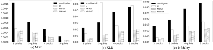
SUPPLEMENTARY FIG. 4: Experimental QREM results with two to five qubits for reducing (a) MSE, (b) KLD and (c) infidelity. Filled bars represent unmitigated results, unfilled bars represent the LI-QREM results, hatched bars represent the NN-QREM results with the full training dataset, and dotted bars represent the NN-QREM results results with the number of training dataset reduced by half.

Num. of qubits	2	3	4	5
$R_{\mathrm{MSE}}$	9.77	8.79	38.0	12.8
$R_{\mathrm{KLD}}$	133	411	53.5	179
$R_{\mathrm{IF}}$	26.9	68.1	44.9	44.0

SUPPLEMENTARY TABLE 1: Performance improvement ratio $R_{i}$ for all metrics tested in this work (i.e. MSE, KLD and IF) for each number of qubits. The number of training data for NN-QREM is a factor of two smaller than that used in the experiment presented in the main manuscript.

References

- [1] Seth Lloyd. Universal quantum simulators. Science, 273(5278):1073–1078, 1996.
- [2] Christof Zalka. Simulating quantum systems on a quantum computer. Proceedings of the Royal Society of London. Series A: Mathematical, Physical and Engineering Sciences, 454(1969):313–322, 1998.
- [3] Peter W Shor. Polynomial-time algorithms for prime factorization and discrete logarithms on a quantum computer. SIAM review, 41(2):303–332, 1999.
- [4] Aram W. Harrow, Avinatan Hassidim, and Seth Lloyd. Quantum algorithm for linear systems of equations. Phys. Rev. Lett., 103:150502, Oct 2009.
- [5] John Preskill. Quantum Computing in the NISQ era and beyond. Quantum, 2:79, August 2018.
- [6] Peter W Shor. Scheme for reducing decoherence in quantum computer memory. Physical review A, 52(4):R2493, 1995.
- [7] Andrew M Steane. Error correcting codes in quantum theory. Physical Review Letters, 77(5):793, 1996.
- [8] A Robert Calderbank and Peter W Shor. Good quantum error-correcting codes exist. Physical Review A, 54(2):1098, 1996.
- [9] Austin G Fowler, Matteo Mariantoni, John M Martinis, and Andrew N Cleland. Surface codes: Towards practical large-scale quantum computation. Physical Review A, 86(3):032324, 2012.
- [10] Barbara M. Terhal. Quantum error correction for quantum memories. Rev. Mod. Phys., 87:307–346, Apr 2015.
- [11] Guanru Feng, Joel J. Wallman, Brandon Buonacorsi, Franklin H. Cho, Daniel K. Park, Tao Xin, Dawei Lu, Jonathan Baugh, and Raymond Laflamme. Estimating the coherence of noise in quantum control of a solid-state qubit. Phys. Rev. Lett., 117:260501, Dec 2016.
- [12] Chao Song, Jing Cui, H. Wang, J. Hao, H. Feng, and Ying Li. Quantum computation with universal error mitigation on a superconducting quantum processor. Science Advances, 5(9), 2019.
- [13] Suguru Endo, Simon C. Benjamin, and Ying Li. Practical quantum error mitigation for near-future applications. Phys. Rev. X, 8:031027, Jul 2018.
- [14] Kristan Temme, Sergey Bravyi, and Jay M. Gambetta. Error mitigation for short-depth quantum circuits. Phys. Rev. Lett., 119:180509, Nov 2017.
- [15] Changjun Kim, Kyungdeock Daniel Park, and June-Koo Rhee. Quantum error mitigation with artificial neural network. IEEE Access, 8:188853–188860, 2020.
- [16] Alberto Peruzzo, Jarrod McClean, Peter Shadbolt, Man-Hong Yung, Xiao-Qi Zhou, Peter J. Love, Alán Aspuru-Guzik, and Jeremy L. O’Brien. A variational eigenvalue solver on a photonic quantum processor. Nature Communications, 5(1):4213, July 2014.
- [17] Jarrod R McClean, Jonathan Romero, Ryan Babbush, and Alán Aspuru-Guzik. The theory of variational hybrid quantum-classical algorithms. New Journal of Physics, 18(2):023023, feb 2016.
- [18] Abhinav Kandala, Antonio Mezzacapo, Kristan Temme, Maika Takita, Markus Brink, Jerry M. Chow, and Jay M. Gambetta. Hardware-efficient variational quantum eigensolver for small molecules and quantum magnets. Nature, 549(7671):242–246, September 2017.
- [19] George S. Barron and Christopher J. Wood. Measurement error mitigation for variational quantum algorithms, 2020.
- [20] Edward Farhi, Jeffrey Goldstone, and Sam Gutmann. A quantum approximate optimization algorithm, 2014.
- [21] Vojtech Havlícek, Antonio D. Córcoles, Kristan Temme, Aram W. Harrow, Abhinav Kandala, Jerry M. Chow, and Jay M. Gambetta. Supervised learning with quantum-enhanced feature spaces. Nature, 567(7747):209–212, 2019.
- [22] Carsten Blank, Daniel K. Park, June-Koo Kevin Rhee, and Francesco Petruccione. Quantum classifier with tailored quantum kernel. npj Quantum Information, 6(1):41, May 2020.
- [23] Daniel K. Park, Carsten Blank, and Francesco Petruccione. The theory of the quantum kernel-based binary classifier. Physics Letters A, 384(21):126422, 2020.
- [24] Carsten Blank, Daniel K. Park, and Francesco Petruccione. Quantum-enhanced analysis of discrete stochastic processes. npj Quantum Information, 7(1):126, August 2021.
- [25] Matthew Ho, Ryuji Takagi, and Mile Gu. Enhancing quantum models of stochastic processes with error mitigation. arXiv:2105.06448 [quant-ph], 2021.
- [26] Abraham Asfaw et al. Learn quantum computation using qiskit, 2020.
- [27] Yanzhu Chen, Maziar Farahzad, Shinjae Yoo, and Tzu-Chieh Wei. Detector tomography on ibm quantum computers and mitigation of an imperfect measurement. Phys. Rev. A, 100:052315, Nov 2019.
- [28] Filip B. Maciejewski, Zoltán Zimborás, and Michał Oszmaniec. Mitigation of readout noise in near-term quantum devices by classical post-processing based on detector tomography. Quantum, 4:257, April 2020.
- [29] Benjamin Nachman, Miroslav Urbanek, Wibe A. de Jong, and Christian W. Bauer. Unfolding quantum computer readout noise. npj Quantum Information, 6(1):84, September 2020.
- [30] Kathleen E. Hamilton, Tyler Kharazi, Titus Morris, Alexander J. McCaskey, Ryan S. Bennink, and Raphael C. Pooser. Scalable quantum processor noise characterization. In 2020 IEEE International Conference on Quantum Computing and Engineering (QCE), pages 430–440, 2020.
- [31] Sergey Bravyi, Sarah Sheldon, Abhinav Kandala, David C. Mckay, and Jay M. Gambetta. Mitigating measurement errors in multiqubit experiments. Phys. Rev. A, 103:042605, Apr 2021.
- [32] Alistair W. R. Smith, Kiran E. Khosla, Chris N. Self, and M. S. Kim. Qubit readout error mitigation with bit-flip averaging. Science Advances, 7(47):eabi8009, 2021.
- [33] Michael R Geller and Mingyu Sun. Toward efficient correction of multiqubit measurement errors: pair correlation method. Quantum Science and Technology, 6(2):025009, feb 2021.
- [34] H. Kwon and J. Bae. A hybrid quantum-classical approach to mitigating measurement errors in quantum algorithms. IEEE Transactions on Computers, pages 1–1, 2020.
- [35] Andrea Morello, Jarryd J. Pla, Patrice Bertet, and David N. Jamieson. Donor spins in silicon for quantum technologies. Advanced Quantum Technologies, 3(11):2000005, 2020.
- [36] Diederik P Kingma and Jimmy Ba. Adam: A method for stochastic optimization. arXiv preprint arXiv:1412.6980, 2014.
- [37] MD SAJID ANIS et al. Qiskit: An open-source framework for quantum computing, 2021.
- [38] Y. Nesterov. A method for solving the convex programming problem with convergence rate . Proceedings of the USSR Academy of Sciences, 269:543–547, 1983.