Quantum Monte Carlo simulations of highly frustrated magnets in a cluster basis: The two-dimensional Shastry-Sutherland model
Abstract
Quantum Monte Carlo (QMC) simulations constitute nowadays one of the most powerful methods to study strongly correlated quantum systems, provided that no “sign problem” arises. However, many systems of interest, including highly frustrated magnets, suffer from an average sign that is close to zero in standard QMC simulations. Nevertheless, a possible sign problem depends on the simulation basis, and here we demonstrate how a suitable choice of cluster basis can be used to eliminate or at least reduce the sign problem in highly frustrated magnets that were so far inaccessible to efficient QMC simulations. We focus in particular on the application of a two-spin (dimer)-based QMC method to the thermodynamics of the spin-1/2 Shastry-Sutherland model for SrCu2(BO3)2.
1 Introduction
Quantum many-body systems constitute a challenge for a quantitatively accurate treatment. In this context, Quantum Monte Carlo (QMC) methods have become one of the most powerful tools [1, 2, 3]. However, in some cases, including geometrically frustrated magnets, their use is limited by a phenomenon known as the “sign problem”, namely a cancellation of positive and negative weights of configurations [4, 5, 6]. In the present contribution, we illustrate how these problems can be overcome or at least alleviated by working in a suitable cluster basis [7, 8, 9, 10]. For the purpose of simplicity, we will focus on the application of a dimer basis to a highly frustrated two-dimensional spin-1/2 model known as the “Shastry-Sutherland model” [11] that is realised in the compound SrCu2(BO3)2 [12, 13].
2 Method and the Shastry-Sutherland model
One flexible QMC approach is based on the representation of the partition function as a high-temperature series [14, 15], leading to the “stochastic series expansion” (SSE). The SSE is based on a splitting of the Hamiltonian into bond terms . These terms are split in turn into different types, such that the action of each bond term on a given basis state either vanishes or yields exactly one other basis state . Note that one of the types is diagonal while all others are off-diagonal. Using , one finds in the given basis
| (1) |
where is the inverse temperature (we set the Boltzmann constant ). Important developments concern the representation and efficient Monte Carlo sampling of the sum in Eq. (1), as well as measurement of physical quantities, and we refer to Refs. [16, 17, 18, 10] for detailed discussions of these issues.
Here, our main concern will be a different one: the weights of a configuration in Eq. (1) are given by products of matrix elements and there is in general no guarantee that they are non-negative, i.e., that the expression Eq. (1) does indeed have a probabilistic interpretation. For diagonal terms of the Hamiltonian, one can add a constant shift to render non-negative. When off-diagonal terms are negative, one uses the absolute value of the weights for sampling such that the average of an observable is given as the ratio of the averages of the observable and of the sign [1, 4],
| (2) |
This allows one to run a QMC simulation for any given problem. However, if indeed negative contributions appear in the sum in Eq. (1), there is a cancellation of negative and positive contributions to , and if these are comparable in magnitude one may not be able to distinguish the normalisation from zero within the error bars of the calculation, thus rendering the results meaningless. This problem is known as the “sign problem”, and we will provide some examples in section 3. Nevertheless, because the sign of the terms in Eq. (1) depends on the choice of basis, one may be able to eliminate or at least alleviate it by a simulation basis that is suitably chosen for a given problem, and we will illustrate one such approach in the following.
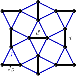
In order to be specific, we will now focus on the Shastry-Sutherland model, which is represented schematically in Fig. 1. The Hamiltonian in the single-site basis is
| (3) |
where are spin-1/2 operators for site . is the intra-dimer coupling (denoted by ) and the inter-dimer coupling () corresponds to a square lattice, as shown in Fig. 1. This model was constructed [11] to ensure that the ground state is an exact product of singlets formed on the dimer bonds for small and intermediate coupling ratios . More recently, this model was also found to be realised in the quantum spin system SrCu2(BO3)2 [12, 13], which increased the interest in calculating its thermodynamic properties.
As a consequence of the triangular arrangement of the and interactions, this problem is geometrically frustrated. Consequently, QMC simulations in the single-spin basis (3) suffer from a severe sign problem, as we will show in section 3. However, one may pass to the total-spin and spin-difference operators, respectively and , for the two spins and on a given dimer [19]. The coupling of the two spins in dimer can then be expressed through and the inter-dimer coupling for the two dimers and indicated in Fig. 1 takes the form
| (4) |
The first term corresponds just to a composite-spin model on a square lattice, which is unfrustrated and thus poses no QMC sign problem. The sign of the coefficient of the second term in Eq. (4) depends on the assignment of the labels and in dimer and varies for the different inter-dimer coupling terms throughout the lattice. There are also signs involved in the construction of the operator such that it is not immediately clear to which extent this second term may still give rise to a sign problem. Nevertheless, the operator yields dimer triplet states when applied to the singlet state of the dimer , . Because the ground state is an exact product of such dimer singlets for , one may expect the difference operators not to contribute to the leading orders at low temperatures, such that a potential sign problem remains manageable. We will show in the next section that indeed this turns out to be true in the regime where is not too large.
3 Results
We now present some QMC results for the Shastry-Sutherland model where we will focus on the two representative cases and .
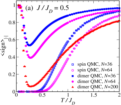
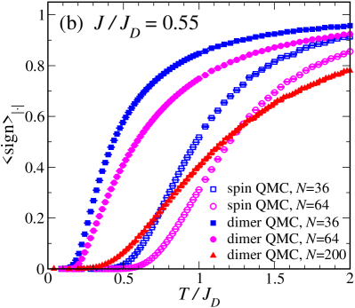
Figure 2 presents the average sign . In the single-spin basis (open symbols), the geometric frustration leads to the expected sign problem (see section 2), which manifests itself as the rapid drop of the average sign at low temperatures. If a sign problem arises, the average sign generically becomes exponentially small in [1, 4]. This is verified by the single-site results, where the average sign not only drops at low temperatures but also decreases with increasing system size . Working in the dimer basis improves the sign problem very significantly, as is illustrated by the full symbols in Fig. 2. There is still a sign problem, as evidenced by the regime in which . However, for and spins, the average sign is always bigger in the dimer basis than in the single-site basis. Most remarkably, at least in the case (Fig. 2(a)) the average sign does not vanish as temperature goes to zero, but instead recovers after going through a minimum around . This minimum still drops with increasing , but one can go to systems as large as and still ensure that , such that the resulting loss of accuracy can be compensated by improving the statistics.
At (Fig. 2(b)), the average sign no longer recovers for , even in the dimer basis. This difference between the cases and can be traced to an algorithmic phase transition at [19], where the effective model defined by the absolute value of the weights in Eq. (2) undergoes a transition out of the dimer phase. Nevertheless, in the dimer basis for spins retains a larger value than that in the single-site basis for the much smaller system at temperatures , as shown in Fig. 2(b).
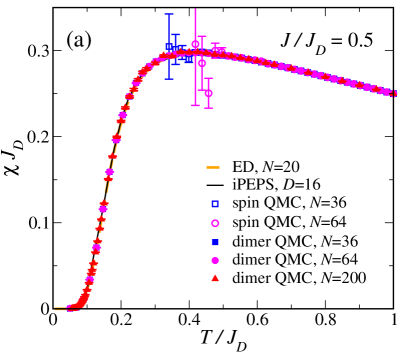
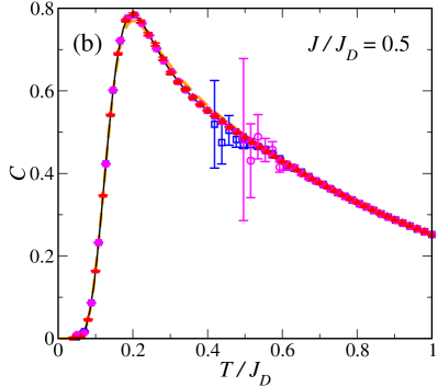
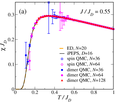
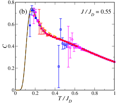
Next we present results for thermodynamic observables at and which are shown respectively in Figs. 3 and 4. As before, QMC results in the single-spin basis are shown by open symbols and results obtained in the dimer basis by filled symbols. For reference, we have included exact diagonalisation (ED) results for spins [19] and infinite projected entangled-pair states (iPEPS) data for a bond dimension [20]. As thermodynamic observables we have selected the magnetic susceptibility and specific heat ; the temperature window is chosen to include the maximum of these two quantities.
The single-site basis is barely able to resolve the maximum of at (Fig. 3(a)) or get close to it for (Fig. 4(a)), provided that one restricts a system size as small as . However, single-site QMC generally loses accuracy already at significantly higher temperatures, such that the maxima are out of reach and only the high-temperature regime is accessible, as was to be expected according to the average sign shown in Fig. 2. On the other hand, for , the dimer basis allows one to obtain accurate QMC data for systems with up to spins and at all temperatures, as shown in Fig. 3. For , the sign problem of Fig. 2(b) prevents one from reaching the zero-temperature limit, but the maximum of the magnetic susceptibility can still be well resolved in the dimer basis for spins (Fig. 4(a)). In order to resolve the maximum of (Fig. 4(b)) by QMC in the dimer basis, one needs to compromise on system size, i.e., restrict to , and on accuracy, but even still works significantly better in the dimer basis than in the single-spin basis, again as expected from the results for the average sign shown in Fig. 2.
The iPEPS data for can be considered as representative of the thermodynamic limit in the present parameter regime and at the level of resolution in Figs. 3 and 4 [20]. Indeed, all of our QMC results agree with iPEPS within the corresponding statistical error bars. On the other hand, small (albeit distinct) finite-size effects can be seen in the ED data, in particular around the maximum of and at temperatures above it. These finite-size effects become increasingly pronounced at the larger value (Fig. 4(b)). This highlights the importance of having access to larger systems in order to ensure quantitatively accurate results.
Concerning the physics of these thermodynamic quantities, we observe the emergence of low-temperature maxima in the magnetic susceptibility and the specific heat that move to lower temperature and sharpen as increases [19, 20]. In the present results, this is seen most clearly for the specific heat, shown in Figs. 3(b) and 4(b).
4 Conclusion
We have shown how a dimer basis can be used to perform accurate QMC simulations for the thermodynamic properties of a highly frustrated two-dimensional spin-1/2 model, the Shastry-Sutherland model, that would be out of reach of conventional approaches. The compound SrCu2(BO3)2 is believed to correspond to the parameter ratio [13, 20]. This ratio is still in the dimer phase of the Shastry-Sutherland model, but rather far beyond the algorithmic phase transition at [19]. Thus the parameter regime relevant to SrCu2(BO3)2 remains unfortunately inaccessible to accurate QMC simulations even in the dimer basis, and one needs to resort to other methods such as iPEPS [20, 21].
Still, there are other cases to which the ideas illustrated here can be applied. For example, in the case of a frustrated ladder, only boundary terms contribute to the sign problem, such that it remains sufficiently mild to allow for a detailed study of the entire phase diagram [8, 22]. Another case is a fully frustrated bilayer model, where the counterpart of the term in Eq. (4) is absent and thus the dimer basis eliminates the sign problem completely [9, 23, 24]. A detailed QMC study of the phase diagram then becomes possible, allowing one to trace a first-order phase transition from zero temperature to finite temperature until it terminates at an Ising critical point [24, 21].
The cluster-basis approach is is not restricted to dimers and we have demonstrated recently that it also works with a trimer (three-spin) basis [10]. This permits one to generalise the investigation of the fully frustrated bilayer model to a trilayer analogue, and study for example the influence of the ground-state entropy that arises in the latter model on the slope of the first-order line at finite temperatures [10].
We would like to thank Bruce Normand for numerous collaborations on related problems and for a critical reading of the manuscript.
References
References
- [1] Evertz H G 2003 Adv. Phys. 52 1–66 URL https://doi.org/10.1080/0001873021000049195
- [2] Troyer M, Alet F, Trebst S and Wessel S 2003 AIP Conf. Proc. 690 156–169 URL https://doi.org/10.1063/1.1632126
- [3] Sandvik A W 2010 AIP Conf. Proc. 1297 135–338 URL https://doi.org/10.1063/1.3518900
- [4] Troyer M and Wiese U J 2005 Phys. Rev. Lett. 94 170201 URL https://doi.org/10.1103/PhysRevLett.94.170201
- [5] Hangleiter D, Roth I, Nagaj D and Eisert J 2020 Sci. Adv. 6 eabb8341 URL https://doi.org/10.1126/sciadv.abb8341
- [6] Hen I 2021 Phys. Rev. Research 3 023080 URL https://doi.org/10.1103/PhysRevResearch.3.023080
- [7] Nakamura T 1998 Phys. Rev. B 57 R3197–R3200 URL https://doi.org/10.1103/PhysRevB.57.R3197
- [8] Honecker A, Wessel S, Kerkdyk R, Pruschke T, Mila F and Normand B 2016 Phys. Rev. B 93 054408 URL https://doi.org/10.1103/PhysRevB.93.054408
- [9] Alet F, Damle K and Pujari S 2016 Phys. Rev. Lett. 117 197203 URL https://doi.org/10.1103/PhysRevLett.117.197203
- [10] Weber L, Honecker A, Normand B, Corboz P, Mila F and Wessel S 2021 (Preprint 2105.05271v4) URL https://arxiv.org/abs/2105.05271v4
- [11] Shastry B S and Sutherland B 1981 Physica B+C 108 1069–1070 URL https://doi.org/10.1016/0378-4363(81)90838-X
- [12] Kageyama H, Yoshimura K, Stern R, Mushnikov N V, Onizuka K, Kato M, Kosuge K, Slichter C P, Goto T and Ueda Y 1999 Phys. Rev. Lett. 82 3168–3171 URL https://doi.org/10.1103/PhysRevLett.82.3168
- [13] Miyahara S and Ueda K 2003 J. Phys.: Condens. Matter 15 R327–R366 URL https://doi.org/10.1088/0953-8984/15/9/201
- [14] Handscomb D C 1964 Math. Proc. Cambridge Phil. Soc. 60 115–122 URL https://doi.org/10.1017/S030500410003752X
- [15] Sandvik A W 1992 J. Phys. A: Math. Gen. 25 3667–3682 URL https://doi.org/10.1088/0305-4470/25/13/017
- [16] Syljuåsen O F and Sandvik A W 2002 Phys. Rev. E 66 046701 URL https://doi.org/10.1103/PhysRevE.66.046701
- [17] Syljuåsen O F 2003 Phys. Rev. E 67 046701 URL https://doi.org/10.1103/PhysRevE.67.046701
- [18] Alet F, Wessel S and Troyer M 2005 Phys. Rev. E 71 036706 URL https://doi.org/10.1103/PhysRevE.71.036706
- [19] Wessel S, Niesen I, Stapmanns J, Normand B, Mila F, Corboz P and Honecker A 2018 Phys. Rev. B 98 174432 URL https://doi.org/10.1103/PhysRevB.98.174432
- [20] Wietek A, Corboz P, Wessel S, Normand B, Mila F and Honecker A 2019 Phys. Rev. Research 1 033038 URL https://doi.org/10.1103/PhysRevResearch.1.033038
- [21] Larrea Jiménez J, Crone S P G, Fogh E, Zayed M E, Lortz R, Pomjakushina E, Conder K, Läuchli A M, Weber L, Wessel S, Honecker A, Normand B, Rüegg C, Corboz P, Rønnow H M and Mila F 2021 Nature 592 370–375 URL https://doi.org/10.1038/s41586-021-03411-8
- [22] Wessel S, Normand B, Mila F and Honecker A 2017 SciPost Phys. 3 005 URL https://doi.org/10.21468/SciPostPhys.3.1.005
- [23] Ng K K and Yang M F 2017 Phys. Rev. B 95 064431 URL https://doi.org/10.1103/PhysRevB.95.064431
- [24] Stapmanns J, Corboz P, Mila F, Honecker A, Normand B and Wessel S 2018 Phys. Rev. Lett. 121 127201 URL https://doi.org/10.1103/PhysRevLett.121.127201