Pearson’s goodness-of-fit tests for sparse distributions

Shuhua Chang^a,b, Deli Li^c, Yongcheng Qi^d

^aCoordinated Innovation Center for Computable Modeling in Management Science, Yango University, Fujian 350015, China

^bCoordinated Innovation Center for Computable Modeling in Management Science, Tianjin University of Finance and Economics, Tianjin 300222, China
Email: szhang@tjufe.edu.cn

^cDepartment of Mathematical Sciences, Lakehead University Thunder Bay, Ontario, Canada P7B 5E1.
Email: dli@lakeheadu.ca

^dDepartment of Mathematics and Statistics, University of Minnesota Duluth, 1117 University Drive, Duluth, MN 55812, USA.
Email: yqi@d.umn.edu

Abstract. Pearson’s chi-squared test is widely used to test the goodness of fit between categorical data and a given discrete distribution function. When the number of sets of the categorical data, say $k$, is a fixed integer, Pearson’s chi-squared test statistic converges in distribution to a chi-squared distribution with $k-1$ degrees of freedom when the sample size $n$ goes to infinity. In real applications, the number $k$ often changes with $n$ and may be even much larger than $n$. By using the martingale techniques, we prove that Pearson’s chi-squared test statistic converges to the normal under quite general conditions. We also propose a new test statistic which is more powerful than chi-squared test statistic based on our simulation study. A real application to lottery data is provided to illustrate our methodology.

Keywords:  Goodness-of-fit; discrete distribution; sparse distribution; normal approximation; chi-square approximation

AMS 2020 Mathematics Subject Classification: 62E20

1 Introduction

Consider an experiment which can result in $k$ possible events, say, $E_{1},\cdots,E_{k}$, where $k\geq 2$ is an integer and $E_{1},\cdots,E_{k}$ form a partition of the sample space. Repeat the experiment $n$ times independently and let $o_{i}$ denote the observed frequency of event $E_{i}$ for $i\in\{1,\cdots,k\}$. Then $(o_{1},\cdots,o_{k})$ has a multinomial distribution. To test the null hypothesis that the probabilities for events $E_{1},\cdots,E_{k}$ are equal to $p_{1},\cdots,p_{k}$, respectively, where $p_{1},\cdots,p_{k}$ are $k$ specified positive numbers with $p_{1}+\cdots+p_{k}=1$, define the following chi-squared test statistic

$$\mathcal{X}^{2}_{n}=\sum^{k}_{i=1}\frac{(o_{i}-e_{i})^{2}}{e_{i}},$$ (1.1)

where $e_{i}=np_{i}$ is the expected number of events $E_{i}$ to occur in the $n$ trials of the experiment for $i\in\{1,\cdots,k\}$. The limiting distribution of $\mathcal{X}^{2}_{n}$ is a chi-squared distribution with $k-1$ degrees of freedom when $k$ is a fixed integer. This is the well-known chi-squared goodness-of-fit test proposed by Pearson [15]. A test with approximate size $\alpha$ rejects the null hypothesis if $\mathcal{X}^{2}_{n}>\chi^{2}_{k-1}(\alpha)$, where $\chi^{2}_{k-1}(\alpha)$ denotes the $\alpha$-level critical value of a chi-squared distribution with $k-1$ degrees of freedom for $\alpha\in(0,1)$.

As a statistical method, Pearson’s chi-squared goodness-of-fit test is one of the most popular topics offered in college statistics courses. The above testing problem can be restated in a different form. Let $f_{0}$ be a discrete probability mass function defined over $\{x_{i},1\leq i\leq k\}$ and set $p_{i}=f_{0}(x_{i})$ for $1\leq i\leq k$. Assume that a random sample of size $n$, $X_{1},\cdots,X_{n}$, is drawn from the distribution of a discrete random variable $X$, where $X$ is a discrete random variable having a probability mass function $f(x)$ for $x=x_{1},\cdots,x_{k}$. Now we can define $E_{i}=\{x_{i}\}$ for $1\leq i\leq k$ and set $o_{i}=\sum^{n}_{j=1}I(X_{j}\in E_{i})$ for $1\leq i\leq k$, and $e_{i}=np_{i}$. Then Pearson’s test statistic $\mathcal{X}^{2}_{n}$ defined in (1.1) can be used to test hypothesis $H_{0}:\leavevmode\nobreak\ f=f_{0}$; i.e. $f(x_{i})=f_{0}(x_{i})$ for $1\leq i\leq k$. Traditionally, Pearson’s chi-squared goodness-of-fit test is suggested to use only if the value of $k$ is relatively small compared with the sample size $n$. When there are infinite many values for a discrete random variable $X$ or the number of distinct values of $X$ is too large compared with the sample size $n$, one can first select a proper integer $k$ and then re-group values of $X$ into $k$ categories by putting the values of $X$ with small probabilities (under the null hypothesis) into one category. When $f_{0}$ is a probability density function, one can discretize the variable $X$ so that Pearson’s chi-squared goodness-of-fit test can be used to test whether the density function of $X$ is equal to $f_{0}$.

When a probability function or density function $f_{0}$ is not fully specified, that is, $f_{0}$ depends some unknown parameters, say $\boldsymbol{\theta}$, the probabilities $p_{1},\cdots,p_{k}$ depend on $\boldsymbol{\theta}$. We can replace $\boldsymbol{\theta}$ with some estimators such as the maximum likelihood estimator, then $\mathcal{X}^{2}_{n}$ still converges in distribution to a chi-squared distribution with $k-r-1$ degrees of freedom where $r$ is the dimension of $\boldsymbol{\theta}$. For more topics and their developments related to Pearson’s test statistics, we refer to Voinov et al. [19].

When the sample size $n$ is small or $k$ is relatively large, some expected frequencies $e_{i}$ may become too small. A variety of estimates of the discrete probability distribution of Pearson’s test statistics have been discussed in the literature, see, e.g. Cochran [2], Yarnold [20], Larntz [11], Lawal [12], Hutchinson [8] and references therein. Baglivo et al. [1] derived formulas for the exact distributions and significance levels of Pearson’s goodness of fit test statistics. Cressie and Read [4] provided a comprehensive review for Pearson’s goodness-of-fit test and the likelihood ratio test.

In this paper, we are interested in the goodness-of-fit test when both $n$ and $k$ go to infinity, that is, we allow that $k=k_{n}$ changes with $n$ and $k_{n}$ can be even much larger than $n$. We note that asymptotic normality of Pearson’s chi-squared test statistics has been obtained by Tumanyan [18] and Holst [7] when $n/k_{n}\to a\in(0,\infty)$ and some restrictive conditions are held. A recent work by Rempała and Wesołowski [17] extended this scope by imposing conditions on the following decomposition of Pearson’s test statistics:

$$\mathcal{X}^{2}_{n}=S_{n1}+S_{n2},\leavevmode\nobreak\ \mbox{ where }S_{n1}=\sum^{k_{n}}_{i=1}\frac{(o_{i}-e_{i})^{2}}{e_{i}}-\sum^{k_{n}}_{i=1}\frac{o_{i}-e_{i}}{e_{i}},\leavevmode\nobreak\ S_{n2}=\sum^{k_{n}}_{i=1}\frac{o_{i}-e_{i}}{e_{i}}.$$ (1.2)

By assuming that $S_{n2}$ is negligible, Rempała and Wesołowski [17] showed that $\mathcal{X}^{2}_{n}$ is asymptotically normal if $n^{2}/k_{n}\to\infty$ as $n\to\infty$. The conditions imposed in Rempała and Wesołowski [17] will be discussed further in Section 2. Since the negligibility condition is trivially true for equiprobable cells, that is, $p_{1}=\cdots=p_{k_{n}}$, $\mathcal{X}^{2}_{n}$ has a normal limit, and furthermore, Rempała and Wesołowski [17] showed in this case that $\mathcal{X}^{2}_{n}$, after properly normalized, converges in distribution to a Poisson distribution if $n^{2}/k_{n}\to\lambda\in(0,\infty)$.

Pearson’s chi-squared test has been proven to be unbiased if one uses equiprobable cells, see, e.g. Mann and Wald [13] and Cohen and Sackrowitz [3]. Koehler and Larntz [9] provided empirical evidence for the accuracy of the normal approximation when $n^{2}/k_{n}$ is reasonably large.

If one does not use equiprobable cells, Haberman [6] noted that Pearson’s test can be biased when some expected frequencies become too small. And this is the case if $k_{n}$ is too large compared with $n$. To overcome this drawback, Zelterman [21, 22] proposed to use $D^{2}$ statistic for the test, i.e. $S_{n1}$ in the decomposition (1.2). Kim et al. [10] compared some asymptotic properties of $\mathcal{X}^{2}_{n}$ statistic and $D^{2}$ statistic for large sparse multinomial distributions.

In this paper, we investigate the limiting distribution for Pearson’s goodness-of-fit test statistic $\mathcal{X}^{2}_{n}$ and $D^{2}$ statistic. By using the decomposition (1.2) for Pearson’s goodness-of-fit test statistic we propose some new test statistics which are more powerful in general.

The rest of the paper is organized as follows. In Section 2, we investigate the limiting distributions of Pearson’s goodness-of-fit test statistics and new test statistics. In Section 3, we carry out a simulation study to compare the performance of these test statistics in terms of the size and the power of the tests. In Section 4, we apply Pearson’s goodness-of-fit test statistics to test whether the winning numbers from Minnesota Lottery Game Daily 3 were randomly selected with equal probabilities. Then we summarize the paper with some concluding remarks. All proofs are given in the Supplement.

2 Main results

Throughout, we always assume that $k=k_{n}\to\infty$ as $n\to\infty$. We adopt some notations as follows. The symbol $\stackrel{{\scriptstyle d}}{{\rightarrow}}$ denotes the convergence in distribution, $N(0,1)$ denotes a standard normal random variable, and $\Phi(x)=(2\pi)^{-1/2}\int^{x}_{-\infty}e^{-t^{2}/2}dt$ is the cumulative distribution function of the standard normal. We also define

$$\sigma^{2}_{n1}=\frac{2(k_{n}-1)(n-1)}{n},\leavevmode\nobreak\ \leavevmode\nobreak\ \sigma_{n2}^{2}=\frac{1}{n}\big{(}\sum^{k_{n}}_{i=1}\frac{1}{p_{i}}-k_{n}^{2}\big{)},\leavevmode\nobreak\ \leavevmode\nobreak\ \leavevmode\nobreak\ \sigma_{n}^{2}=\sigma_{n1}^{2}+\sigma_{n2}^{2},$$ (2.1)

where $\sigma_{n}^{2}$, $\sigma_{n1}^{2}$ and $\sigma_{n2}^{2}$ are the variances of $\mathcal{X}^{2}_{n}$, $S_{n1}$ and $S_{n2}$, respectively. In Read and Cressie [16], the first three asymptotic moments have been derived for the so-called power-divergence statistics which include Pearson’s $\mathcal{X}^{2}_{n}$ statistic as a special case.

We need to impose the following conditions in deriving the limiting distributions for Pearson’s test statistic $\mathcal{X}^{2}_{n}$ and some new test statistics that we will propose in the paper:

We first investigate the asymptotic properties of $S_{n1}$ (i.e. $D^{2}$ statistic) and $\mathcal{X}_{n}^{2}$.

$$\frac{1}{n^{2}k_{n}^{2}}\sum^{k_{n}}_{i=1}\frac{1}{p_{i}^{2}}\to 0\mbox{ as }n\to\infty,$$ (2.2)

$$\min\Big{(}\frac{\sum^{k_{n}}_{i=1}\frac{1}{p_{i}^{3}}-k_{n}^{4}}{n^{3}\sigma_{n2}^{4}}I(\sigma_{n2}^{2}>0),\frac{\sigma_{n2}^{2}}{k_{n}}\Big{)}\to 0\mbox{ as }n\to\infty.$$ (2.3)

Theorem 2.1.

If (2.2) holds, then we have

$$\frac{S_{n1}-(k_{n}-1)}{\sigma_{n1}}\stackrel{{\scriptstyle d}}{{\rightarrow}}N(0,1)\leavevmode\nobreak\ \leavevmode\nobreak\ \leavevmode\nobreak\ \mbox{ as }n\to\infty,$$ (2.4)

where $\sigma_{n1}$ is defined in (2.1).

Theorem 2.2.

Under conditions (2.2) and (2.3) we have

$$\frac{\mathcal{X}^{2}_{n}-(k_{n}-1)}{\sigma_{n}}\stackrel{{\scriptstyle d}}{{\rightarrow}}N(0,1)\leavevmode\nobreak\ \leavevmode\nobreak\ \leavevmode\nobreak\ \mbox{ as }n\to\infty,$$ (2.5)

where $\sigma_{n}$ is defined in (2.1).

Based on the normal approximation (2.5), a test with approximate size $\alpha$ rejects the null hypothesis if $\mathcal{X}^{2}_{n}>k_{n}-1+\sigma_{n}z_{\alpha}$, where $z_{\alpha}$ denotes the $\alpha$-level critical value of the standard normal distribution for each $\alpha\in(0,1)$. Based on (2.4), a test with approximate size $\alpha$ rejects the null hypothesis if $S_{n1}>k_{n}-1+\sigma_{n1}z_{\alpha}$.

A test of size $\alpha$ is said to be unbiased if the power of the test is at least $\alpha$ under alternative hypotheses. The test based on the statistic $\mathcal{X}^{2}_{n}$ is not unbiased under some alternatives as pointed out by Haberman [6]. More seriously, our simulation study indicates that the test has a nearly zero power under some alternatives, that is, the test loses its power completely in those cases; see Table 2. In order to understand why this happens, we will look at the decomposition (1.2) for the goodness-of-fit test statistic $\mathcal{X}^{2}_{n}$. From Lemma A.1 in the Supplement, we have under the null hypothesis $P(E_{i})=p_{i}$ for $1\leq i\leq k_{n}$ that

$$\mathbb{E}(S_{n1}-(k_{n}-1))=0\mbox{ and }\mathbb{E}(S_{n2})=0,$$

and under the alternative $H_{1}$: $P(E_{i})=p_{i}^{\prime}$ for $1\leq i\leq k_{n}$ that

$$\mathbb{E}\big{(}S_{n1}-(k_{n}-1)|H_{1}\big{)}=(n-1)\sum^{k_{n}}_{i=1}\frac{(p_{i}^{\prime}-p_{i})^{2}}{p_{i}}\leavevmode\nobreak\ \mbox{ and }\leavevmode\nobreak\ \mathbb{E}(S_{n2}|H_{1})=\sum^{k_{n}}_{i=1}\frac{p_{i}^{\prime}-p_{i}}{p_{i}}.$$ (2.6)

The variances under $H_{1}$ can be calculated for both $S_{n1}$ and $S_{n2}$. Since the rejection region of the goodness-of-fit test is one-sided, the test gains its power from a shift to right in location of the test statistic $\mathcal{X}^{2}_{n}$ under the alternative. In $S_{n1}$, the effect of a shift is always positive, but the sign of $\sum^{k_{n}}_{i=1}\frac{p_{i}^{\prime}-p_{i}}{p_{i}}$, the location shift in $S_{n2}$, can be negative. If this shift in location to left in $S_{n2}$ is overwhelming, the observed values for $\mathcal{X}^{2}_{n}$ can be very small and will result in rejecting the alternative hypotheses.

Since we are considering the situation when both $n$ and $k_{n}$ are large, from (2.6), $|\mathbb{E}(S_{n2}|H_{1})|$ can be very large compared with $\mathbb{E}\big{(}S_{n1}-(k_{n}-1)|H_{1}\big{)}$ when $k_{n}$ is much larger than $n$. This indicates that using $|S_{n2}|$ in the test statistics can be more powerful than $S_{n2}$. We propose a class of test statistics $S_{n1}+c|S_{n2}|$, where $c\geq 0$ is a constant. Their limiting distributions are given as follows.

Theorem 2.3.

Under conditions (2.2) and (2.3) we have as $n\to\infty$

$$\sup_{x}\Big{|}P\Big{(}\frac{S_{n1}+c|S_{n2}|-(k_{n}-1)}{\sigma_{n1}}\leq x\Big{)}-P\Big{(}Z_{1}+\frac{c\sigma_{n2}}{\sigma_{n1}}|Z_{2}|\leq x\Big{)}\Big{|}\to 0,$$ (2.7)

where $Z_{1}$ and $Z_{2}$ are independent random variables with the standard normal distribution, and $c\geq 0$ is any given constant.

For each $s$, define $\Psi(x,s)$ as the cumulative distribution function of $Z_{1}+s|Z_{2}|$, i.e.

$$\Psi(x,s)=P(Z_{1}+s|Z_{2}|\leq x)=\sqrt{\frac{2}{\pi}}\int^{\infty}_{0}\Phi(x-st)\exp(-t^{2}/2)dt.$$ (2.8)

For each $\alpha\in(0,1)$, let $\psi_{\alpha}(s)$ denote an $\alpha$-level critical value of $\Psi(\cdot,s)$, that is, $1-\Psi(\psi_{\alpha}(s),s)=\alpha$. The integral in (2.8) has no close form solution but it can be evaluated numerically by using function ‘integrate’ in R. Critical values $\psi_{\alpha}(s)$ can be solved via the Newton-Raphson method. Note that $\Psi(x,0)=\Phi(x)$ and thus $\psi_{\alpha}(0)=z_{\alpha}$ for $\alpha\in(0,1)$.

Three test statistics, $S_{n1}$, $\mathcal{X}_{n}^{2}$, and $S_{n1}+c|S_{n2}|$ with $c\geq 0$, can be used to test the null hypothesis that $P(E_{i})=p_{i}$ for $1\leq i\leq k_{n}$, and their rejection regions at level $\alpha$, according to equations (2.4), (2.5) and (2.7), are given by

$$\mathcal{R}_{0}=\Big{\{}S_{n1}>k_{n}-1+\sigma_{n1}z_{\alpha}\Big{\}},$$

$$\mathcal{R}=\Big{\{}\mathcal{X}_{n}^{2}>k_{n}-1+\sigma_{n}z_{\alpha}\Big{\}},$$ (2.9)

and

$$\mathcal{R}_{c}=\Big{\{}S_{n1}+c|S_{n2}|>k_{n}-1+\sigma_{n1}\psi_{\alpha}(\frac{c\sigma_{n2}}{\sigma_{n1}})\Big{\}}$$ (2.10)

for $c\geq 0$. Note that test $\mathcal{R}_{0}$ can be considered as a special case of $\mathcal{R}_{c}$ defined in (2.10) with $c=0$.

The aforementioned test statistics (or their corresponding rejection regions) are the same when $p_{1}=\cdots=p_{k_{n}}$ since $\sigma_{n2}^{2}=0$ and $S_{n2}=0$ in this case. Note that Theorem 2.1 can be considered as a special case of Theorem 2.3 with $c=0$, but in Theorem 2.1 we impose only condition (2.2) which is less restrictive than conditions in Theorem 2.3. If we assume $p_{1}=\cdots=p_{k_{n}}$, condition (2.2) is equivalent to $\lim_{n\to\infty}k_{n}/n^{2}=0$. Immediately we have the following corollary.

Corollary 2.1.

Assume that $\{k_{n}\}$ is a sequence of positive integers such that $k_{n}\to\infty$ and $k_{n}=o(n^{2})$ as $n\to\infty$. Then under the assumption that $p_{1}=\cdots=p_{k_{n}}$, we have

$$\frac{\mathcal{X}^{2}_{n}-(k_{n}-1)}{\sigma_{n1}}\stackrel{{\scriptstyle d}}{{\rightarrow}}N(0,1)\leavevmode\nobreak\ \mbox{ as }\leavevmode\nobreak\ n\to\infty.$$

Under the assumption of the equiprobable cells with $p_{1}=\cdots=p_{k_{n}}$, we have $S_{n2}=0=\sum^{k_{n}}_{i=1}\frac{o_{i}-e_{i}}{e_{i}}$ for any samples, regardless of how large for any single term $\frac{o_{i}-e_{i}}{e_{i}}$. As a remedy, we can assign a weight for each term such that the weighted sum is not degenerate. Now we introduce a weighted version for $S_{n2}$ as follows

$$\overline{S}_{n2}=\sum^{k_{n}}_{i=1}\frac{c_{i}(o_{i}-e_{i})}{e_{i}},$$ (2.11)

where $c_{i}\geq 0$ for $1\leq i\leq k_{n}$ and $\sum^{k_{n}}_{i=1}c_{i}=k_{n}$. Obviously, $S_{n2}$ is a special case of $\overline{S}_{n2}$ with $c_{1}=\cdots=c_{k_{n}}=1$.

We can verify that

$$\overline{\sigma}_{n2}^{2}=\mathbb{E}(\overline{S}_{n2}^{2})=\frac{1}{n}\Big{(}\sum^{k_{n}}_{i=1}\frac{c_{i}^{2}}{p_{i}}-k_{n}^{2}\Big{)}\leavevmode\nobreak\ \mbox{ and }\leavevmode\nobreak\ \mathbb{E}(\overline{S}_{n2})=0;$$ (2.12)

see (A.31) in the Supplement.

Now we propose a new class of test statistics $S_{n1}+c|\overline{S}_{n2}|$, where $c\geq 0$ is a constant. We need the following condition for the asymptotic normality for those test statistics.

$$\min\Big{(}\frac{\sum^{k_{n}}_{i=1}\frac{c_{i}^{4}}{p_{i}^{3}}-k_{n}^{4}}{n^{3}\overline{\sigma}_{n2}^{4}}I(\overline{\sigma}_{n2}^{2}>0),\frac{\overline{\sigma}_{n2}^{2}}{k_{n}}\Big{)}\to 0\mbox{ as }n\to\infty.$$ (2.13)

Theorem 2.4.

Under conditions (2.2) and (2.13) we have as $n\to\infty$

$$\sup_{x}\Big{|}P\Big{(}\frac{S_{n1}+c|\overline{S}_{n2}|-(k_{n}-1)}{\sigma_{n1}}\leq x\Big{)}-P\Big{(}Z_{1}+\frac{c\overline{\sigma}_{n2}}{\sigma_{n1}}|Z_{2}|\leq x\Big{)}\Big{|}\to 0,$$ (2.14)

where $Z_{1}$ and $Z_{2}$ are independent random variables with the standard normal distribution, and $c\geq 0$ is any given constant.

For given weights $c_{1},\cdots,c_{k_{n}}$ and constant $c\geq 0$, a test of size $\alpha$ based on approximation (2.14) for test statistic $S_{n1}+c|\overline{S}_{n2}|$ has the following rejection region

$$\overline{\mathcal{R}}_{c}=\{S_{n1}+c|\overline{S}_{n2}|>k_{n}-1+\sigma_{n1}\psi_{\alpha}(\frac{c\overline{\sigma}_{n2}}{\sigma_{n1}})\},$$ (2.15)

where $\overline{\sigma}_{n2}$ is defined in (2.12).

Of particular interest, we offer a discussion for the selection on weights $c_{1},\cdots,c_{k_{n}}$ so that $\overline{S}_{n2}$ is non-degenerate and condition (2.13) is satisfied for the equiprobable cells. When $p_{1}=\cdots=p_{k_{n}}=\frac{1}{k_{n}}$, we select weights $c_{1},\cdots,c_{k_{n}}$ such that they are not identically equal to $1$. This ensures $\overline{\sigma}_{n2}^{2}>0$.

A very simple way is to select an integer $k_{0}$ such that $k_{0}\sim hk_{n}$ for some $h\in(0,1)$ and assign a value $k_{n}/k_{0}$ to $k_{0}$ of $c_{i}$’s and $0$ to the remaining $k_{n}-k_{0}$ weights. Then for any integer $r\geq 1$, we have

$$\sum^{k_{n}}_{i=1}\frac{c_{i}^{r+1}}{p_{i}^{r}}-k_{n}^{r+1}=k_{n}^{r}k_{0}\big{(}\frac{k_{n}}{k_{0}}\big{)}^{r+1}-k_{n}^{r+1}=\Big{(}\big{(}\frac{k_{n}}{k_{0}}\big{)}^{r}-1\Big{)}k_{n}^{r+1}\sim\big{(}h^{-r}-1\big{)}k_{n}^{r+1}.$$

Then the first term in the parentheses in (2.13) approximately equals

$$\frac{(h^{-3}-1)k_{n}^{4}}{n\big{(}(h^{-1}-1)k_{n}^{2}\big{)}^{2})}\sim\frac{h^{-3}-1}{(h^{-1}-1)^{2}}\frac{1}{n}\to 0$$

as $n\to\infty$. That is, (2.13) holds.

3 A simulation study

In this section, we compare the performance of the test statistics defined in Section 2 through some simulations.

We first compare the sizes and powers of the test statistics $\mathcal{X}_{n}^{2}$, $S_{n1}$ and $S_{n1}+c|S_{n2}|$ under some general null hypotheses. Then we compare the performance of $\mathcal{X}_{n}^{2}$ and $S_{n1}+c|\overline{S}_{n2}|$ under equiprobable cells with $p_{1}=\cdots=p_{k_{n}}$.

Firstly, we consider the following five tests, including $\mathcal{R}$, $\mathcal{R}_{0}$, $\mathcal{R}_{1}$, $\mathcal{R}_{3}$ and $\mathcal{R}_{5}$ as defined in (2.9) and (2.10) with selection of $\alpha=0.05$ and several combinations of $n$ and $k_{n}$. For each case, the simulation is repeated $10000$ times by using R package, and the sizes and powers of these tests are estimated.

We assume $k_{n}$ is an even integer and define

$$p_{1}=\cdots=p_{\frac{k_{n}}{2}}=\frac{r}{k_{n}},\leavevmode\nobreak\ \leavevmode\nobreak\ p_{\frac{k_{n}}{2}+1}=\cdots=p_{k_{n}}=\frac{2-r}{k_{n}}$$ (3.1)

for $r\in(0,2)$. For given $n$ and $k_{n}$, each of the above probability distributions is uniquely determined by $r$. We note that $p_{1}=\cdots=p_{k_{n}}=\frac{1}{k_{n}}$ if and only if $r=1$.

Table 1 contains estimated sizes for the five tests $\mathcal{R}$, $\mathcal{R}_{0}$, $\mathcal{R}_{1}$, $\mathcal{R}_{3}$ and $\mathcal{R}_{5}$ with $n=100$, $1000$ and some selected values for $k_{n}$. For each combination of ($n$, $k_{n})$, we take three probability distributions from (3.1) with $r=0.1$, $0.2$, $0.6$ and $1.0$, respectively. When $r=1.0$, all the five tests are the same. From Table 1 the estimated sizes for all five tests are very close to the nominal level $0.05$, and thus, we conclude all the five tests perform very well in terms of the accuracy in type I error.

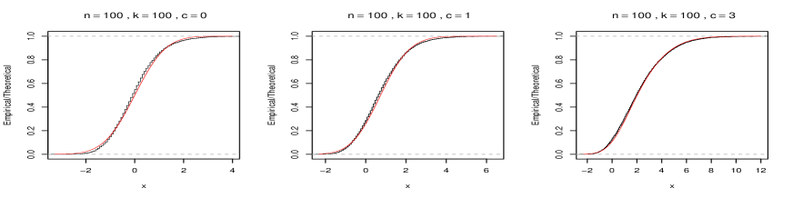
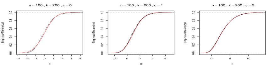
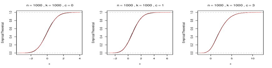
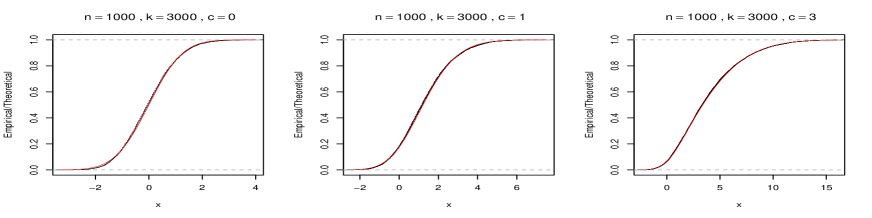
Figure 1: Plots of the empirical distribution for the standardized test statistics $(S_{n1}+c|S_{n2}|-(k_{n}-1))/\sigma_{n1}$ and their theoretical limiting cumulative distribution $\Psi(x,c\sigma_{n2}/\sigma_{n1})$ under the null hypothesis from family (3.1) with $r=0.2$. $\Psi$ is defined in (2.8). We select $c=0,1,$ and $3$, corresponding to the tests $\mathcal{R}_{0}$, $\mathcal{R}_{1}$ and $\mathcal{R}_{3}$. In these plots, the red/smooth lines represent the theoretical cumulative distributions $\Psi(x,c\sigma_{n2}/\sigma_{n1})$.

To assess the overall performance of the distributional approximations to the standardized test statistics $(S_{n1}+c|S_{n2}|-(k_{n}-1))/\sigma_{n1}$ under the null hypothesis, we compare the empirical distributions of the test statistics based on 10000 samples and their theoretical cumulative distribution functions under the null hypothesis with a distribution from family (3.1). Figure 1 contains plots for both the empirical distributions and the approximate distributions of the test statistics with $c=0$, $1$, $3$. The parameter of the distribution under $H_{0}$ is set to be $r=0.2$. We discover from Figure 1 that all three theoretical distributions for the test statistics fit the empirical distributions very well, and their accuracies improve when sample size is getting large. Results for other distributions are similar and are not reported here.

To estimate the power for these tests, for each combination of $n$ and $k_{n}$, we choose probability distribution (3.1) as the null hypothesis with $r=0.2$ (or $r=0.6$), and use probability distribution (3.1) with $r=0.2\pm 0.1$ (or accordingly, $r=0.6\pm 0.1$) as alternative hypotheses from which random samples are generated. Table 2 lists the estimated powers for the five tests. Surprisingly, the power of test $\mathcal{R}$ is nearly zero when the value of $r$ in the true alternative hypothesis is smaller than the value of $r$ specified in the null hypothesis, that is, Pearson’s goodness-of-fit test is seriously biased in those cases. As we have explained below equation (1.2), this is mainly due to $\sum^{k_{n}}_{i=1}\frac{p_{i}^{\prime}-p_{i}}{p_{i}}$. For example, if $r=0.2$ for the distribution under the null hypothesis and $r=0.1$ under the alternative, we have

$$\sum^{k_{n}}_{i=1}\frac{p_{i}^{\prime}-p_{i}}{p_{i}}=(\frac{-0.1}{0.2}+\frac{0.1}{1.8})\frac{k_{n}}{2}=-\frac{2k_{n}}{9}.$$

We can also estimate the standard deviation of $\mathcal{X}^{2}_{n}$ under the alternative hypothesis and find out that it is much smaller than order $k_{n}$. This explains the incapability of Pearson’s goodness-of-fit test in detecting an alternative in this case. We also notice that the performance of $\mathcal{R}$ is quite regular when $r=0.2$ for the distribution under the null hypothesis and $r=0.3$ under the alternative. Since $\sum^{k_{n}}_{i=1}\frac{p_{i}^{\prime}-p_{i}}{p_{i}}=\frac{2k_{n}}{9}>0$ in this case, Pearson’s goodness-of-fit test gains its power. In both examples, the power of test $\mathcal{R}_{c}$ increases with $c$. In the first example, test $\mathcal{R}_{c}$ is superior to $\mathcal{R}$ for all $c\geq 0$. In the second example, test $\mathcal{R}_{c}$ outperforms $\mathcal{R}$ when $c\geq 3$.

It seems plausible that test $\mathcal{R}_{c}$ with $c>0$ improves upon $\mathcal{R}$ when $\sum^{k_{n}}_{i=1}\frac{p_{i}^{\prime}-p_{i}}{p_{i}}$ is quite different from zero. It is interesting to know how much improvement can be made when $\sum^{k_{n}}_{i=1}\frac{p_{i}^{\prime}-p_{i}}{p_{i}}$ is zero or very close to zero. To make an empirical comparison, we introduce a new family of probability distributions. For convenience, we assume that $k_{n}$ is divisible by $4$ and define a family of probability distributions

$$p_{1}^{\prime}=\cdots=p_{\frac{k_{n}}{4}}^{\prime}=\frac{1.5r^{\prime}}{k_{n}},\leavevmode\nobreak\ p_{\frac{k_{n}}{4}+1}^{\prime}=\cdots=p_{\frac{k_{n}}{2}}^{\prime}=\frac{0.5r^{\prime}}{k_{n}},\leavevmode\nobreak\ p_{\frac{k_{n}}{2}+1}^{\prime}=\cdots=p_{k_{n}}^{\prime}=\frac{2-r^{\prime}}{k_{n}}$$ (3.2)

for $r^{\prime}\in(0,2)$. For given $n$ and $k_{n}$, each probability distribution above is uniquely determined by $r^{\prime}$. It is easy to see that for a probability distribution $(p_{1},\cdots,p_{k_{n}})$ from (3.1) and a probability distribution $(p_{1}^{\prime},\cdots,p_{k_{n}}^{\prime})$ from (3.2), $\sum^{k_{n}}_{i=1}\frac{p_{i}^{\prime}-p_{i}}{p_{i}}=0$ if $r=r^{\prime}$. Table 3 includes estimated powers of the five tests for several combinations of $n$ and $k_{n}$ with $r=r^{\prime}=0.6$, $1.4$. The probability distribution under the null hypothesis is from family (3.1) with parameter $r$ and the true probability distribution under the alternative is from (3.2) with parameter $r^{\prime}=r$. From Table 3, the power of $\mathcal{R}_{c}$ decreases with $c$ for large $c$. We note that the constant $c$ represents the weight of $|S_{n2}|$ we take into account in the test, and $S_{n1}$ has always a positive shift in location under the alternative, and thus it is more likely to detect the alternative if the weight of $|S_{n2}|$ in the test is smaller. In other words, increasing the weight $c$ can decrease the power of $\mathcal{R}_{c}$ in this case. Therefore, we do not recommend to use a large $c$ in general. In Table 3, we have used least favorable distributions to the use of $S_{n2}$ under alternatives since the expectations of $S_{n2}$ under the alternatives are zero. Overall, the performance of test $\mathcal{R}_{0}$ is slightly better than test $\mathcal{R}_{1}$ from Table 3.

Now we compare $\mathcal{X}_{n}^{2}$ and $S_{n1}+c|\overline{S}_{n2}|$ for the case of equiprobable cells. Recall that $\mathcal{X}_{n}=S_{n1}$ in this case. We define $\overline{S}_{n2}$ by using the method discussed at the end of Section 2, that is, we define $k_{0}=0.8k_{n}$ and set $c_{i}=\frac{k_{n}}{k_{0}}=\frac{1}{0.8}=1.25$ for $1\leq i\leq k_{0}$ and $0$ otherwise. This time, we consider only two tests, $\mathcal{R}_{0}$ and $\overline{\mathcal{R}}_{1}$, as defined in (2.9) and (2.15) with $c=1$. For several combinations of $n$ and $k_{n}$, the sizes for the two tests are estimated based on $10000$ replicates. The powers for the two tests are also estimated when the distributions under the alternatives are from family (3.1) with $r=0.8$, $1.2$ and $1.4$ or from family (3.2) with $r^{\prime}=0.8$, $1.1$ and $1.2$. The estimated sizes and powers are reported in Table 4.

From Table 4, we conclude that the sizes for both $\mathcal{R}_{1}$ and $\overline{\mathcal{R}}_{1}$ are close to the nominal level $0.05$, and in general, $\overline{\mathcal{R}}_{1}$ is more powerful than $\mathcal{R}_{1}$. These empirical results are consistent with Theorem 2.4, and adding the term $\overline{S}_{n2}$ defined in (2.11), a non-trivial linear combination of the terms $(o_{i}-e_{i})/e_{i}$, can improve the power of the test significantly.

Next, we extend our comparison of $S_{n1}$ and $S_{n1}+c|\overline{S}_{n2}|$ to some none-equiprobable cases. We also use the method discussed at the end of Section 2 to define $\overline{S}_{n2}$ by setting $k_{0}=0.40k_{n}$ this time. We consider the distributions from family (3.2) and use the same settings as in Table 3. Only for an illustration purpose, we demonstrate the weighted test statistics can improve the power of the test $\mathcal{R}_{1}$ when the expectation of $S_{n2}$ under $H_{1}$ in (2.6) is zero. Both the sizes and powers for tests $\mathcal{R}_{0}$ and $\mathcal{R}_{1}$ are reported in Table 5. From the table, we see that both the tests maintain reasonable sizes for all combinations of $n$ and $k_{n}$. From Tables 3 and 5, we can conclude that test $\overline{\mathcal{R}}_{1}$ performs significantly better than $\mathcal{R}_{0}$ and $\mathcal{R}_{1}$ in terms of power.

Finally, we compare the performance of these tests under sparsity. To this end, we introduce a class of distributions as follows

$$p_{1}=\cdots=p_{0.95k_{n}}=\frac{r}{8k_{n}},\leavevmode\nobreak\ \leavevmode\nobreak\ p_{0.95k_{n}+1}=\cdots=p_{k_{n}}=\frac{160-19r}{8k_{n}}$$ (3.3)

for $r\in(0,8)$, where $k_{n}$ is a multiple of $20$. We see that only $5\%$ of probabilities $p_{i}$’s take a larger value $\frac{160-19r}{8k_{n}}$ in (3.3). In our study, we select $r=2$ for the distribution under the null hypothesis and estimate the sizes of the five tests considered in Table 1 and estimate the powers of the tests under the alternatives $r=1$ and $r=3$ for some combinations of $n$ and $k_{n}$. The estimated sizes and powers are reported in Table 6.

Results in Table 6 are quite similar to Tables 1 and 2 in the following aspects: a. the estimated type I errors are close to nominal level $0.05$ for all five tests; b. Pearson’s test $\mathcal{R}$ loses its power totally for some distributions under the alternative while tests $\mathcal{R}_{1}$, $\mathcal{R}_{3}$, and $\mathcal{R}_{5}$ outperform with large powers. Although test $\mathcal{R}_{0}$ is better than Pearson’s test, its overall performance is not quite satisfactory. For example, for some distributions under the alternative, its powers are smaller than the type I errors. We examine the results in Table 6 when $n=100$ with $r=1$ under the alternative and find out that the power of the test decreases from $0.0416$ to $0.0246$ when $k_{n}$ increases from $100$ to $400$. The same phenomenon can also be observed when $n=1000$.

It is worth mentioning that conditions (2.2) and (2.3) that ensure the asymptotic normality of $S_{n1}$ and $\mathcal{X}^{2}_{n}$ may be moderately violated if $k_{n}$ is too large compared with $n$. This is the case for some combinations of $n$ and $k_{n}$ and for some distributions used in Table 6. In our study, the sizes (type I errors) of all five tests are reasonably close to the nominal level $0.05$; see Tables 1 and 6. In terms of power, test $\mathcal{R}_{1}$, $\mathcal{R}_{3}$, and $\mathcal{R}_{5}$ are also very robust as they gain good powers from Tables 2 and 6.

To conclude this section, we present more discussion on selection of $c$. Our simulation study indicates that there is no answer for optimal section of $c$ in general. As we have pointed out, $c$ represents the weight of $|S_{n2}|$ in test $\mathcal{R}_{c}$. When $c$ is large, the test $\mathcal{R}_{c}$ is almost the same as $\{|S_{n2}|/\sigma_{n2}>z_{\alpha/2}\}$, where $z_{\alpha/2}$ is the $\alpha/2$-level critical value of the standard normal distribution. On the one hand, the power of test $\mathcal{R}_{c}$ increases with $c$ in most cases in Tables 2 and 6. By comparing the powers of the test $\mathcal{R}_{c}$ for various values of $c$ in our simulation study, we find out that the increment in the power for the test $\mathcal{R}_{c}$ is very limited when $c$ is larger than $3$, and the power of $\mathcal{R}_{2}$ is close to that of $\mathcal{R}_{3}$ in most cases. On the other hand, Table 3 indicates that one may prefer to employ a test $\mathcal{R}_{c}$ with a smaller value $c$ in the worst scenarios such as those distributions given in (3.2). We observe from Table 3 that the power of $\mathcal{R}_{1}$ is very close to that of $\mathcal{R}_{0}$ in most cases. Our simulation study also shows that the power of $\mathcal{R}_{2}$ is only slightly smaller than that of $\mathcal{R}_{1}$ in most cases. Intuitively, the power of test $\mathcal{R}_{c}$ depends on the probability distributions under both the null and alternative hypotheses as well as the relative convergence rate of $n$ and $k_{n}$. A theoretical investigation on how the power function of the test $\mathcal{R}_{c}$ depends on these factors can be very helpful but may be very complicated. In practice, the distributions under the alternative are unknown, and the optimal choice of $c$ that works for all distributions does not exist. To balance different situations, one can use tests $\mathcal{R}_{1}$ or $\mathcal{R}_{2}$. As a general recommendation, one can calculate tests $\mathcal{R}$, $\mathcal{R}_{0}$, $\mathcal{R}_{1}$ and $\mathcal{R}_{2}$ for comparison purpose. One should be cautious about accepting the null hypothesis based on $\mathcal{R}$ or $\mathcal{R}_{0}$ since the powers of the two tests may be much smaller than their sizes or type I errors. In other words, tests $\mathcal{R}$ and $\mathcal{R}_{0}$ may reject the alternative hypotheses with a probability close to one when the null hypotheses are not true.

Table 1: Estimated Sizes of Tests (Nominal Level $\alpha=0.05$): Probability distributions under null hypotheses and the true distributions that are used to generate samples are from family (3.1) with different values for parameter $r$

Sample		Distribution	True	Probability of Rejecting $H_{0}$ for Tests
Size ($n$)	$k_{n}$	under $H_{0}$	distribution	$\mathcal{R}$	$\mathcal{R}_{0}$	$\mathcal{R}_{1}$	$\mathcal{R}_{3}$	$\mathcal{R}_{5}$
100	50	$r=0.1$	$r=0.1$	0.0679	0.0638	0.0642	0.0536	0.0500
100	50	0.2	0.2	0.0663	0.0614	0.0668	0.0633	0.0599
100	50	0.6	0.6	0.0609	0.0593	0.0628	0.0672	0.0674
100	50	1.0	1.0	0.0576	0.0576	0.0576	0.0576	0.0576
100	100	$r=0.1$	$r=0.1$	0.0610	0.0595	0.0569	0.0482	0.0450
100	100	0.2	0.2	0.0667	0.0610	0.0594	0.0567	0.0526
100	100	0.6	0.6	0.0579	0.0562	0.0594	0.0616	0.0642
100	100	1.0	1.0	0.0531	0.0531	0.0531	0.0531	0.0531
100	200	$r=0.1$	$r=0.1$	0.0644	0.0679	0.0567	0.0491	0.0413
100	200	0.2	0.2	0.0619	0.0579	0.0622	0.0536	0.0544
100	200	0.6	0.6	0.0580	0.0550	0.0606	0.0579	0.0539
100	200	1.0	1.0	0.0691	0.0691	0.0691	0.0691	0.0691
1000	300	$r=0.1$	$r=0.1$	0.0571	0.0543	0.0574	0.0521	0.0519
1000	300	0.2	0.2	0.0552	0.0523	0.0567	0.0562	0.0538
1000	300	0.6	0.6	0.0515	0.0518	0.0527	0.0536	0.0556
1000	300	1.0	1.0	0.0514	0.0514	0.0514	0.0514	0.0514
1000	1000	$r=0.1$	$r=0.1$	0.0570	0.0594	0.0583	0.0533	0.0543
1000	1000	0.2	0.2	0.0525	0.0548	0.0526	0.0523	0.0489
1000	1000	0.6	0.6	0.0538	0.0534	0.0526	0.0505	0.0516
1000	1000	1.0	1.0	0.0530	0.0530	0.0530	0.0530	0.0530
1000	3000	$r=0.1$	$r=0.1$	0.0542	0.0600	0.0515	0.0501	0.0505
1000	3000	0.2	0.2	0.0549	0.0568	0.0570	0.0511	0.0510
1000	3000	0.6	0.6	0.0544	0.0546	0.0561	0.0553	0.0532
1000	3000	1.0	1.0	0.0565	0.0565	0.0565	0.0565	0.0565
1000	10000	$r=0.1$	$r=0.1$	0.0485	0.0648	0.0447	0.0468	0.0472
1000	10000	0.2	0.2	0.0544	0.0614	0.0506	0.0493	0.0494
1000	10000	0.6	0.6	0.0520	0.0590	0.0567	0.0491	0.0486
1000	10000	1.0	1.0	0.0567	0.0567	0.0567	0.0567	0.0567

Table 2: Estimated Powers of Tests ($\alpha=0.05$): Probability distributions under null hypotheses and the true distributions that are used to generate samples are from family (3.1) with different values for parameter $r$

Sample		Distribution	True	Probability of Rejecting $H_{0}$ for Tests
Size ($n$)	$k_{n}$	under $H_{0}$	distribution	$\mathcal{R}$	$\mathcal{R}_{0}$	$\mathcal{R}_{1}$	$\mathcal{R}_{3}$	$\mathcal{R}_{5}$
100	50	$r=0.1$	$r=0.05$	0.0042	0.0455	0.1044	0.1408	0.1315
100	50	0.2	0.1	0.0041	0.0677	0.1998	0.3646	0.3864
100	50	0.2	0.3	0.3207	0.1377	0.2608	0.3679	0.3884
100	50	0.6	0.5	0.0436	0.0699	0.0909	0.1316	0.1614
100	50	0.6	0.7	0.1247	0.0856	0.1066	0.1463	0.1768
100	200	$r=0.1$	$r=0.05$	0.0025	0.0372	0.1120	0.1096	0.0893
100	200	0.2	0.1	0.0010	0.0413	0.2627	0.3577	0.3730
100	200	0.2	0.3	0.3890	0.1156	0.3178	0.3831	0.3935
100	200	0.6	0.5	0.0231	0.0573	0.0924	0.1526	0.1743
100	200	0.6	0.7	0.1399	0.0723	0.1111	0.1678	0.1946
1000	300	$r=0.1$	$r=0.05$	0.0000	0.0936	0.7955	0.9723	0.9823
1000	300	0.2	0.1	0.0001	0.2739	0.9465	0.9996	1.0000
1000	300	0.2	0.3	0.8806	0.3361	0.8425	0.9876	0.9951
1000	300	0.6	0.5	0.0369	0.1202	0.2360	0.5269	0.7207
1000	300	0.6	0.7	0.2917	0.1464	0.2591	0.5150	0.6971
1000	1000	$r=0.1$	$r=0.05$	0.0000	0.0577	0.9308	0.9825	0.9856
1000	1000	0.2	0.1	0.0000	0.1123	0.9937	0.9999	1.0000
1000	1000	0.2	0.3	0.9678	0.2041	0.9463	0.9953	0.9968
1000	1000	0.6	0.5	0.0072	0.0814	0.2860	0.7165	0.8531
1000	1000	0.6	0.7	0.3585	0.1000	0.2880	0.6896	0.8311
1000	3000	$r=0.1$	$r=0.05$	0.0000	0.0423	0.9741	0.9874	0.9880
1000	3000	0.2	0.1	0.0000	0.0657	0.9996	1.0000	1.0000
1000	3000	0.2	0.3	0.9951	0.1545	0.9902	0.9974	0.9979
1000	3000	0.6	0.5	0.0004	0.0632	0.4394	0.8597	0.9174
1000	3000	0.6	0.7	0.5278	0.0826	0.4314	0.8272	0.8948
1000	10000	$r=0.1$	$r=0.05$	0.0000	0.0431	0.9838	0.9883	0.9891
1000	10000	0.2	0.1	0.0000	0.0476	1.0000	1.0000	1.0000
1000	10000	0.2	0.3	0.9974	0.1292	0.9952	0.9967	0.9969
1000	10000	0.6	0.5	0.0000	0.0575	0.7122	0.9226	0.9377
1000	10000	0.6	0.7	0.7677	0.0777	0.6766	0.8997	0.9165

Table 3: Estimated Powers of Tests ($\alpha=0.05$): Probability distributions under null hypotheses and the true distributions that are used to generate samples are from family (3.1) with parameter $r$ and family (3.2) with parameter $r^{\prime}$, respectively

Sample		Distribution	Distribution	Probability of Rejecting $H_{0}$ for Tests
Size ($n$)	$k_{n}$	under $H_{0}$	under $H_{1}$	$\mathcal{R}$	$\mathcal{R}_{0}$	$\mathcal{R}_{1}$	$\mathcal{R}_{3}$	$\mathcal{R}_{5}$
100	100	$r=$0.6	$r^{\prime}=$0.6	0.1562	0.1511	0.1536	0.1400	0.1173
100	100	1.4	1.4	0.3179	0.3418	0.3386	0.2895	0.2168
100	200	$r=$0.6	$r^{\prime}=$0.6	0.1197	0.1238	0.1215	0.0992	0.0808
100	200	1.4	1.4	0.1940	0.2260	0.2241	0.1647	0.1185
1000	300	$r=$0.6	$r^{\prime}=$0.6	0.8606	0.8739	0.8716	0.8513	0.8083
1000	300	1.4	1.4	0.9999	1.0000	1.0000	1.0000	1.0000
1000	1000	$r=$0.6	$r^{\prime}=$0.6	0.4694	0.4939	0.4833	0.4016	0.2968
1000	1000	1.4	1.4	0.9713	0.9758	0.9721	0.9403	0.8441
1000	3000	$r=$0.6	$r^{\prime}=$0.6	0.2252	0.2575	0.2370	0.1556	0.1104
1000	3000	1.4	1.4	0.6195	0.7019	0.6605	0.4225	0.2482
1000	10000	$r=$0.6	$r^{\prime}=$0.6	0.1156	0.1547	0.1292	0.0794	0.0671
1000	10000	1.4	1.4	0.2212	0.3412	0.2761	0.1275	0.0924

Table 4: Estimated Sizes and Powers for Tests $\mathcal{R}_{0}$ and $\overline{\mathcal{R}}_{1}$ for Equiprobable Cells ($\alpha=0.05$). The distributions under alternatives are from family (3.1) with parameter $r$ and from family (3.2) with parameter $r^{\prime}$, respectively

Sample				Power under family (3.1)			Power under family (3.2)
Size ($n$)	$k_{n}$	Tests	Sizes	$r=0.8$	$r=1.2$	$r=1.4$	$r^{\prime}=0.8$	$r^{\prime}=1.1$	$r^{\prime}=1.2$
100	100	$\mathcal{R}_{0}$	0.0531	0.0964	0.0900	0.3009	0.2013	0.3030	0.4264
100	100	$\overline{\mathcal{R}}_{1}$	0.0593	0.1306	0.1262	0.4449	0.2544	0.3208	0.4656
100	200	$\mathcal{R}_{0}$	0.0691	0.0976	0.0973	0.2342	0.1830	0.2428	0.3349
100	200	$\overline{\mathcal{R}}_{1}$	0.0604	0.1256	0.1140	0.3720	0.2084	0.2234	0.3450
1000	300	$\mathcal{R}_{0}$	0.0514	0.4804	0.4739	0.9999	0.9978	0.9998	1.0000
1000	300	$\overline{\mathcal{R}}_{1}$	0.0556	0.6341	0.6264	1.0000	0.9990	0.9998	1.0000
1000	1000	$\mathcal{R}_{0}$	0.0530	0.2249	0.2238	0.9515	0.9501	0.9998	0.9945
1000	1000	$\overline{\mathcal{R}}_{1}$	0.0552	0.5072	0.4986	0.9993	0.9604	0.9998	0.9988
1000	3000	$\mathcal{R}_{0}$	0.0565	0.1384	0.1435	0.6444	0.4710	0.6459	0.8444
1000	3000	$\overline{\mathcal{R}}_{1}$	0.0561	0.5650	0.5587	0.9984	0.8342	0.7316	0.9675
1000	10000	$\mathcal{R}_{0}$	0.0567	0.0963	0.0972	0.3176	0.2268	0.3136	0.4599
1000	10000	$\overline{\mathcal{R}}_{1}$	0.0494	0.7127	0.7153	1.0000	0.8199	0.4869	0.9097

Table 5: Estimated Sizes and Powers of Tests $\mathcal{R}_{0}$ and $\overline{\mathcal{R}}_{1}$ ($\alpha=0.05$): Probability distributions under null hypotheses are from family (3.1) with parameter $r$ and the distributions under alternatives are from family (3.2) with parameter $r^{\prime}$

Sample		Distribution	Sizes for Tests		Distribution	Powers for Tests
Size ($n$)	$k_{n}$	under $H_{0}$	$\mathcal{R}_{0}$	$\overline{\mathcal{R}}_{1}$	under $H_{1}$	$\mathcal{R}_{0}$	$\overline{\mathcal{R}}_{1}$
100	100	$r=$0.6	0.0562	0.0612	$r^{\prime}=$0.6	0.1511	0.1844
100	100	1.4	0.0612	0.0665	1.4	0.3418	0.4478
100	200	$r=$0.6	0.0550	0.0515	$r^{\prime}=$0.6	0.1238	0.1525
100	200	1.4	0.0564	0.0606	1.4	0.2260	0.3704
1000	300	$r=$0.6	0.0518	0.0560	$r^{\prime}=$0.6	0.8739	0.9227
1000	300	1.4	0.0537	0.0548	1.4	1.0000	1.0000
1000	1000	$r=$0.6	0.0534	0.0547	$r^{\prime}=$0.6	0.4939	0.7565
1000	1000	1.4	0.0573	0.0560	1.4	0.9758	0.9995
1000	3000	$r=$0.6	0.0546	0.0542	$r^{\prime}=$0.6	0.2575	0.6527
1000	3000	1.4	0.0515	0.0547	1.4	0.7019	0.9949
1000	10000	$r=$0.6	0.0590	0.0497	$r^{\prime}=$0.6	0.1547	0.6164
1000	10000	1.4	0.0576	0.0505	1.4	0.3412	0.9947

Table 6: Estimated Sizes and Powers of Tests under Sparsity (Nominal Level $\alpha=0.05$): Probability distributions under null hypotheses and the true distributions that are used to generate samples are from family (3.3) with different values for parameter $r$

Sample		Distribution	True	Size or	Probability of Rejecting $H_{0}$ for Tests
Size($n$)	$k_{n}$	under $H_{0}$	distribution	power	$\mathcal{R}$	$\mathcal{R}_{0}$	$\mathcal{R}_{1}$	$\mathcal{R}_{3}$	$\mathcal{R}_{5}$
100	100	$r=$2	$r=$2	size	0.0623	0.0607	0.0610	0.0547	0.0509
100	100	2	1	power	0.0000	0.0416	0.7327	0.8545	0.8613
100	100	2	3	power	0.6877	0.2145	0.6008	0.7410	0.7559
100	200	$r=$2	$r=$2	size	0.0609	0.0632	0.0597	0.0516	0.0520
100	200	2	1	power	0.0000	0.0331	0.7878	0.8529	0.8688
100	200	2	3	power	0.7450	0.1899	0.6616	0.7526	0.7626
100	400	2	2	size	0.0584	0.0617	0.0517	0.0476	0.0468
100	400	2	1	power	0.0000	0.0246	0.8237	0.8714	0.8712
100	400	2	3	power	0.7837	0.1690	0.6973	0.7543	0.7611
1000	300	$r=$2	$r=$2	size	0.0598	0.0559	0.0601	0.0547	0.0518
1000	300	2	1	power	0.0000	0.9779	1.0000	1.0000	1.0000
1000	300	2	3	power	0.9999	0.8164	0.9997	1.0000	1.0000
1000	1000	$r=$2	$r=$2	size	0.0582	0.0602	0.0579	0.0540	0.0544
1000	1000	2	1	power	0.0000	0.5604	1.0000	1.0000	1.0000
1000	1000	2	3	power	1.0000	0.5143	1.0000	1.0000	1.0000
1000	3000	$r=$2	$r=$2	size	0.0551	0.0597	0.0536	0.0515	0.0516
1000	3000	2	1	power	0.0000	0.1361	1.0000	1.0000	1.0000
1000	3000	2	3	power	1.0000	0.3219	1.0000	1.0000	1.0000
1000	10000	$r=$2	$r=$2	size	0.0511	0.0633	0.0520	0.0488	0.0487
1000	10000	2	1	power	0.0000	0.0384	1.0000	1.0000	1.0000
1000	10000	2	3	power	1.0000	0.2211	1.0000	1.0000	1.0000

4 A real data application

As an application, we study the winning numbers from the Minnesota Lottery Game Daily 3. The game has been played for many years, and a winning number consisting of three digits is drawn daily. The three digits are drawn from digits $0,1,\cdots,9$. Minnesota Lottery does not reveal how the three digits are selected in its official website. According to the State Lottery Report Card (available at the site https://www.lotterypost.com/lottery-report-card.asp), the winning numbers for Minnesota Daily 3 are drawn by computer programs.

In Game Daily 3, there are $1000$ possible drawing outcomes. We are interested in whether the drawing mechanism for Daily 3 is random, this is, whether all $1000$ possible outcomes are equally likely. Recent winning numbers for this game can be found at the Minnesota Lottery web site https://www.mnlottery.com/games/lotto_games/daily_3/winning_s/. As an application, we examine some early data from Game Daily 3. We have collected a total of $2919$ data points from August 14, 1990 to August 13, 1998. The winning numbers were drawn every day except Christmas days in years 1990, 1991 and 1992. This old dataset was obtained from the official Minnesota lottery website but now it is no longer available. One may find it from https://www.lotterypost.com/results.

Since our null hypothesis is that $p_{1}=\cdots=p_{1000}=1/1000$, all three test statistics, $\mathcal{X}_{n}^{2}$, $S_{n1}$, and $S_{n1}+c|S_{n2}|$, are the same. We first apply all $2919$ data for the test. The observed $\mathcal{X}^{2}_{n}$ is $978.5677$ with mean $999$ and standard deviation $44.69$, and the standardized statistic is $(978.6777-999)/44.69=-0.4572$, which has a p-value $0.6962$. To apply the new test $\overline{\mathcal{R}}_{1}$, we assign a value $1.25$ to these $800$ weights $c_{i}$ to the cells associated to the drawing numbers whose first digits are smaller than $8$. Then we have an observed value $-0.1774$ for $\big{(}S_{n1}+|\overline{S}_{n2}|-(k_{n}-1)\big{)}/\sigma_{n}$, and the corresponding p-value is $0.6927$. Therefore, at the $5\%$ significance level, we couldn’t reject the null hypothesis and conclude that the $1000$ possible winning numbers may be drawn with equal probability.

Next, we test the hypothesis that $p_{1}=\cdots=p_{1000}=1/1000$ based on each of eight periods. A period starts from August 14 in one year and ends next August 13. Namely, Period 1 is from August 14, 1990 to August 13, 1991, and Period 2 is from August 14, 1991 to August 13, 1993, so on. For each of the first seven periods, both tests result in large p-values. For Period 8, that is, during Aug 14, 1997 to Aug 13, 1998, the p-value for test $\mathcal{R}$ is $0.00085$, and the p-value from test $\overline{\mathcal{R}}_{1}$ is $0.002867$. We identify that the data during August 14, 1997 and August 13, 1998 seem highly abnormal. We find out that both winning numbers $(3,7,5)$ and $(4,4,8)$ appeared $4$ times, and each of the other $11$ numbers appeared $3$ times.

Our second test procedure consists of $8$ individual tests. In order to control the overall type I error at the $5\%$ level, we use the Bonferroni inequality for multiple comparisons, that is, we reject the null hypothesis that $p_{1}=\cdots=p_{1000}=1/1000$ at level $0.05$ if any of the $8$ individuals tests is rejected at level $0.05/8=0.00625$. Since both tests $\mathcal{R}$ and $\overline{\mathcal{R}}_{1}$ have a p-value smaller than $0.00625$ for Period 8, we conclude that the hypothesis of equiprobability can be rejected at level $0.05$.

5 Concluding remarks

In this paper, we investigate the performance of Pearson’s goodness-of-fit test when both the number of cells and the sample size go to infinity. Under quite general conditions, we have obtained the limiting distributions for Pearson’s goodness-of-fit test statistic and Zelterman’s $D^{2}$ test statistic. By decomposing Pearson’s test statistic, we propose new test statistics so as to overcome the bias problem of Pearson’s chi-squared test. Our simulation study indicates that test $\mathcal{R}_{1}$ is superior to Pearson’s goodness-of-fit test $\mathcal{R}$ in general. $\mathcal{R}_{1}$ gains a much larger power than $\mathcal{R}$ in most cases and is no longer biased. Our new test $\overline{\mathcal{R}}_{1}$ is also much more powerful than $\mathcal{R}$ for testing the equiprobable cells. For small and moderate sample sizes, as pointed out by a referee, one can apply permutation procedures (Drikvandi et al. [5]) or bootstrap procedures (Nordhausen et al. [14]) to conduct the tests.

Supplementary material

Proofs of the main results in the paper are given in the Supplement.

Disclosure statement

No potential conflict of interest was reported by the authors.

Supplement

Pearson’s goodness-of-fit tests for sparse distributions

Shuhua Chang^a,b, Deli Li^c, Yongcheng Qi^d

^aCoordinated Innovation Center for Computable Modeling in Management Science, Yango University, Fujian 350015, China

^bCoordinated Innovation Center for Computable Modeling in Management Science, Tianjin University of Finance and Economics, Tianjin 300222, China
Email: szhang@tjufe.edu.cn

^cDepartment of Mathematical Sciences, Lakehead University Thunder Bay, Ontario, Canada P7B 5E1.
Email: dli@lakeheadu.ca

^dDepartment of Mathematics and Statistics, University of Minnesota Duluth, 1117 University Drive, Duluth, MN 55812, USA.
Email: yqi@d.umn.edu

Appendix: Proofs of the Main Results

For each $j\in\{1,\cdots,n\}$, define random variable $X_{j}=i$ if $E_{i}$ occurs in the $j$-th trial of the experiment. Then $X_{j},\leavevmode\nobreak\ 1\leq j\leq n$, are independent and identically distributed random variables with $P(X_{j}=i)=p_{i}$ for $1\leq i\leq k_{n}$, $1\leq j\leq n$. Define

$$\delta_{i,j}=I(X_{j}=i)-p_{i}\leavevmode\nobreak\ \leavevmode\nobreak\ \mbox{ for }1\leq i\leq k_{n},\leavevmode\nobreak\ 1\leq j\leq n$$

and set

$$\Delta_{i,\ell}=\sum^{\ell}_{j=1}\delta_{i,j}\leavevmode\nobreak\ \leavevmode\nobreak\ \mbox{ for }1\leq i\leq k_{n},\leavevmode\nobreak\ \leavevmode\nobreak\ 1\leq\ell\leq n.$$

For convenience, set $\Delta_{i,0}=0$ for any $1\leq i\leq k_{n}$.

From now on, we use $\mathbb{E}(\cdot)$ to denote the expectation under the null hypothesis that $P(E_{i})=p_{i}$ for $1\leq i\leq k_{n}$. When an alternative is specified as $H_{1}$: $P(E_{i})=p_{i}^{\prime}$ for $1\leq i\leq k_{n}$, where $(p_{1}^{\prime},\cdots,p_{k_{n}}^{\prime})\neq(p_{1},\cdots,p_{k_{n}})$, $\mathbb{E}(\cdot|H_{1})$ denotes the conditional expectation under $H_{1}$.

We can easily verify the following equations:

$$\mathbb{E}(\delta_{i,j})=0,\leavevmode\nobreak\ \leavevmode\nobreak\ \leavevmode\nobreak\ \mathbb{E}(\delta_{i,j}^{2})=p_{i}(1-p_{i});$$ (A.1)

$$\mathbb{E}(\delta_{i,j}\delta_{i^{\prime},j^{\prime}})=0\leavevmode\nobreak\ \leavevmode\nobreak\ \mbox{ if }j\neq j^{\prime};$$ (A.2)

$$\mathbb{E}(\delta_{i,j}\delta_{i^{\prime},j})=\left\{\begin{array}[]{ll}p_{i}(1-p_{i}),&\hbox{ if }i=i^{\prime};\\ -p_{i}p_{i^{\prime}},&\hbox{ if }i\neq i^{\prime},\end{array}\right.$$ (A.3)

$$\sum_{i=1}^{k_{n}}\delta_{i,j}=0\leavevmode\nobreak\ \leavevmode\nobreak\ \mbox{ and }\leavevmode\nobreak\ \sum_{i=1}^{k_{n}}\Delta_{i,j}=0,$$ (A.4)

where $1\leq i,i^{\prime}\leq k_{n}$, $1\leq j,j^{\prime}\leq n$ in the above equations.

Since $\sum^{\ell}_{j=1}I(X_{j}=i)$ is the sum of $\ell$ independent Bernoulli random variables, its distribution is binomial. We have

$$\mathbb{E}(\Delta_{i,\ell}^{2})=\ell p_{i}(1-p_{i}),\leavevmode\nobreak\ \leavevmode\nobreak\ \leavevmode\nobreak\ 1\leq\ell\leq n.$$ (A.5)

We can also verify that

$$\mathbb{E}(\Delta_{i_{1},\ell}\Delta_{i_{2},\ell})=-\ell p_{i_{1}}p_{i_{2}},\leavevmode\nobreak\ \leavevmode\nobreak\ \leavevmode\nobreak\ 1\leq i_{1}\neq i_{2}\leq k_{n},\leavevmode\nobreak\ \leavevmode\nobreak\ 1\leq\ell\leq n.$$ (A.6)

For each $i\in\{1,\cdots,k_{n}\}$, we have

$$o_{i}=\sum^{n}_{j=1}I(X_{j}=i)\leavevmode\nobreak\ \leavevmode\nobreak\ \leavevmode\nobreak\ \mbox{ and }o_{i}-e_{i}=\sum^{n}_{j=1}\delta_{i,j}=\Delta_{i,n}.$$ (A.7)

We also need the following expectations under the alternative $H_{1}$

$$\mathbb{E}(\delta_{i,j}|H_{1})=p_{i}^{\prime}-p_{i}\leavevmode\nobreak\ \leavevmode\nobreak\ \mbox{ and }\leavevmode\nobreak\ \leavevmode\nobreak\ \mathbb{E}(\delta_{i,j}\delta_{i,j^{\prime}}|H_{1})=(p_{i}^{\prime}-p_{i})^{2}$$ (A.8)

for $1\leq i\leq k_{n}$, $1\leq j\neq j^{\prime}\leq n$.

Lemma A.1.

Let $S_{n1}$ and $S_{n2}$ be defined in (1.2). Then

$$S_{n1}=\frac{1}{n}\sum^{k_{n}}_{i=1}\frac{1}{p_{i}}\sum_{1\leq j_{1}\neq j_{2}\leq n}\delta_{i,j_{1}}\delta_{i,j_{2}}+k_{n}-1$$ (A.9)

and

$$S_{n2}=\frac{1}{n}\sum^{n}_{j=1}\sum^{k_{n}}_{i=1}\frac{\delta_{i,j}}{p_{i}}.$$ (A.10)

Under the null hypothesis that $P(X_{1}=i)=p_{i}$ for $1\leq i\leq k_{n}$, we have

$$\mathbb{E}(S_{n1}-(k_{n}-1))=0,\leavevmode\nobreak\ \leavevmode\nobreak\ \mathbb{E}(S_{n2})=0;$$ (A.11)

Under the alternative $H_{1}$: $P(X_{1}=i)=p_{i}^{\prime}$ for $1\leq i\leq k_{n}$, we have

$$\mathbb{E}\big{(}S_{n1}-(k_{n}-1)|H_{1}\big{)}=(n-1)\sum^{k_{n}}_{i=1}\frac{(p_{i}^{\prime}-p_{i})^{2}}{p_{i}},\leavevmode\nobreak\ \leavevmode\nobreak\ \mathbb{E}(S_{n2}|H_{1})=\sum^{k_{n}}_{i=1}\frac{p_{i}^{\prime}-p_{i}}{p_{i}}.$$ (A.12)

Proof. With the notations in the beginning of the section, (A.10) can be verified easily by using (A.7). To show (A.9), notice that

$$\mathcal{X}^{2}_{n} = \sum^{k_{n}}_{i=1}\frac{(\sum^{n}_{j=1}\delta_{i,j})^{2}}{np_{i}}$$ (A.13)

$$= \frac{1}{n}\sum^{k_{n}}_{i=1}\frac{1}{p_{i}}\sum^{n}_{j_{1}=1}\sum^{n}_{j_{2}=1}\delta_{i,j_{1}}\delta_{i,j_{2}}$$

$$= \frac{1}{n}\sum^{k_{n}}_{i=1}\frac{1}{p_{i}}\sum_{1\leq j_{1}\neq j_{2}\leq n}\delta_{i,j_{1}}\delta_{i,j_{2}}+\frac{1}{n}\sum^{k_{n}}_{i=1}\frac{1}{p_{i}}\sum^{n}_{j=1}\delta_{i,j}^{2}.$$

Since $\delta_{i,j}^{2}=I(X_{j}=i)-2I(X_{j}=i)p_{i}+p_{i}^{2}$, $\sum^{k_{n}}_{i=1}I(X_{j}=i)=1$, and $\sum^{k_{n}}_{i=1}p_{i}=1$, we have

$$\frac{1}{n}\sum^{k_{n}}_{i=1}\frac{1}{p_{i}}\sum^{n}_{j=1}\delta_{i,j}^{2} = \frac{1}{n}\sum^{k_{n}}_{i=1}\sum^{n}_{j=1}\Big{(}\frac{I(X_{j}=i)}{p_{i}}-2I(X_{j}=i)+p_{i}\Big{)}$$

$$= \frac{1}{n}\sum^{n}_{j=1}\sum^{k_{n}}_{i=1}\Big{(}\frac{I(X_{j}=i)}{p_{i}}-2I(X_{j}=i)+p_{i}\Big{)}$$

$$= \frac{1}{n}\sum^{n}_{j=1}\Big{(}\sum^{k_{n}}_{i=1}\frac{I(X_{j}=i)}{p_{i}}-1\Big{)}$$

$$= \frac{1}{n}\sum^{n}_{j=1}\sum^{k_{n}}_{i=1}\frac{I(X_{j}=i)-p_{i}}{p_{i}}+(k_{n}-1)$$

$$= \frac{1}{n}\sum^{n}_{j=1}\sum^{k_{n}}_{i=1}\frac{\delta_{i,j}}{p_{i}}+(k_{n}-1)$$

$$= S_{n2}+k_{n}-1,$$

which, together with (A.13), yields (A.9).

Equations (A.11) and (A.12) follow from (A.9), (A.10), (A.2) and (A.8). This completes the proof. ∎

Lemma A.2.

Let $c_{i}$, $1\leq i\leq k_{n}$, be non-negative numbers with $\sum^{k_{n}}_{i=1}c_{i}=k_{n}$. Then for any $j\geq 1$

$$\beta_{nj}:=\sum^{k_{n}}_{i=1}\frac{c_{i}^{j+1}}{p_{i}^{j}}-k_{n}^{j+1}\geq 0,$$ (A.14)

and the equality holds only if for some $c>0$, $c_{i}=cp_{i}$ for $1\leq i\leq k_{n}$.

Proof. We will prove (A.14) by induction. By using the Cauchy-Schwarz inequality we get

$$\sum^{k_{n}}_{i=1}\frac{c_{i}^{2}}{p_{i}}=\sum^{k_{n}}_{i=1}\big{(}\frac{c_{i}}{p_{i}^{1/2}}\big{)}^{2}\sum^{k_{n}}_{i=1}(p_{i}^{1/2})^{2}\geq\Big{(}\sum^{k_{n}}_{i=1}\frac{c_{i}}{p_{i}^{1/2}}p_{i}^{1/2}\Big{)}^{2}=k_{n}^{2}$$

and the equality holds only if $(\frac{c_{1}}{\sqrt{p_{1}}},\cdots,\frac{c_{k_{n}}}{\sqrt{p_{k_{n}}}})=c(\sqrt{p_{1}},\cdots,\sqrt{p_{k_{n}}})$ for some $c>0$, and the latter is equivalent to $c_{i}=cp_{i}$ for $1\leq i\leq k_{n}$. This implies (A.14) holds with $j=1$. Now assume (A.14) holds for all $j\leq j_{0}$ for some $j_{0}\geq 1$. We need to show (A.14) holds with $j=j_{0}+1$. If $j_{0}+1=2k$ is an even number where $k\geq 1$, then it follows from the Cauchy-Schwarz inequality that

$$\sum^{k_{n}}_{i=1}\frac{c_{i}^{j_{0}+2}}{p_{i}^{j_{0}+1}}=\frac{1}{k_{n}}\sum^{k_{n}}_{i=1}\big{(}\frac{c_{i}^{k+1/2}}{p_{i}^{k}}\big{)}^{2}\sum^{k_{n}}_{i=1}(c_{i}^{1/2})^{2}\geq\frac{1}{k_{n}}\Big{(}\sum^{k_{n}}_{i=1}\frac{c_{i}^{k+1}}{p_{i}^{k}}\Big{)}^{2}\geq\frac{1}{k_{n}}(k_{n}^{k+1})^{2}=k_{n}^{j_{0}+2},$$

and the equality holds only if $c_{i}=cp_{i}$ for $1\leq i\leq k_{n}$ for some $c>0$, proving (A.14) with $j=j_{0}+1$. If $j_{0}+1=2k+1$ is an odd number with $k\geq 1$, then again from the Cauchy-Schwarz inequality

$$\sum^{k_{n}}_{i=1}\frac{c_{i}^{j_{0}+2}}{p_{i}^{j_{0}+1}} = \sum^{k_{n}}_{i=1}\big{(}\frac{c^{k+1}}{p_{i}^{(2k+1)/2}}\big{)}^{2}\sum^{k_{n}}_{i=1}(p_{i}^{1/2})^{2}\geq\Big{(}\sum^{k_{n}}_{i=1}\frac{c_{i}^{k+1}p_{i}^{1/2}}{p_{i}^{(2k+1)/2}}\Big{)}^{2}$$

$$\geq \Big{(}\sum^{k_{n}}_{i=1}\frac{c_{i}^{k+1}}{p_{i}^{k}}\Big{)}^{2}\geq\big{(}k_{n}^{k+1}\big{)}^{2}=k_{n}^{j_{0}+2},$$

i.e. (A.14) holds with $j=j_{0}+1$. Similarly, we have the equality only if $c_{i}=cp_{i}$ for $1\leq i\leq k_{n}$ for some $c>0$. This completes the proof. ∎

Lemma A.3.

Assume $\{n_{r},\leavevmode\nobreak\ r\geq 1\}$ is an increasing sequence of positive integers. If (2.2) holds with $n=n_{r}$ as $r\to\infty$, then (2.4) holds with $n=n_{r}$ as $r\to\infty$.

Proof. For brevity, we will drop the subscript $r$ and write $n_{r}$ as $n$ in the proof.

To prove (2.4), we will employ a martingale technique. To this end, we first rewrite $S_{n1}$ as

$$S_{n1}-(k_{n}-1) = \frac{1}{n}\sum^{k_{n}}_{i=1}\frac{1}{p_{i}}\sum_{1\leq j_{1}\neq j_{2}\leq n}\delta_{i,j_{1}}\delta_{i,j_{2}}$$

$$= \frac{2}{n}\sum^{k_{n}}_{i=1}\frac{1}{p_{i}}\sum_{1\leq j_{1}<j_{2}\leq n}\delta_{i,j_{1}}\delta_{i,j_{2}}$$

$$= \frac{2}{n}\sum^{k_{n}}_{i=1}\frac{1}{p_{i}}\sum^{n}_{\ell=2}\sum_{j=1}^{\ell-1}\delta_{i,j}\delta_{i,\ell}$$

$$= \sum^{n}_{\ell=2}\Big{(}\frac{2}{n}\sum^{k_{n}}_{i=1}\frac{1}{p_{i}}\sum_{j=1}^{\ell-1}\delta_{i,j}\delta_{i,\ell}\Big{)}$$

$$= \sum^{n}_{\ell=2}\Big{(}\frac{2}{n}\sum^{k_{n}}_{i=1}\frac{1}{p_{i}}\Delta_{i,\ell-1}\delta_{i,\ell}\Big{)}.$$

Let $\mathcal{F}_{n\ell}=\sigma(X_{1},X_{2},\cdots,X_{\ell})$ denote the $\sigma$-algebra generated by $\{X_{1},X_{2},\cdots,X_{\ell}\}$ for $1\leq\ell\leq n$, and $\mathcal{F}_{n0}=\{\phi,\Omega\}$ is the trivial $\sigma$-algebra. Now set

$$z_{n\ell}=\frac{2}{n}\sum^{k_{n}}_{i=1}\frac{1}{p_{i}}\Delta_{i,\ell-1}\delta_{i,\ell},\leavevmode\nobreak\ \leavevmode\nobreak\ 1\leq\ell\leq n.$$ (A.15)

Note that $z_{n1}=0$. By the independence of $\delta_{i,\ell}$ and $\mathcal{F}_{n(\ell-1)}$, we have

$$\mathbb{E}(z_{n\ell}|\mathcal{F}_{n(\ell-1)})=\frac{2}{n}\sum^{k_{n}}_{i=1}\frac{1}{p_{i}}\Delta_{i,\ell-1}\mathbb{E}(\delta_{i,\ell}|\mathcal{F}_{n(\ell-1)})=0\leavevmode\nobreak\ \leavevmode\nobreak\ \leavevmode\nobreak\ \mbox{ for }1\leq\ell\leq n.$$

Therefore, $\{z_{n\ell},\leavevmode\nobreak\ \mathcal{F}_{n\ell},\leavevmode\nobreak\ 1\leq\ell\leq n,\leavevmode\nobreak\ n\geq 2\}$ form an array of martingale differences. Since $S_{n1}=\sum^{n}_{\ell=1}z_{n\ell}$, it is sufficient to show that

$$\frac{\sum^{p_{n}}_{\ell=1}z_{n\ell}}{\sigma_{n1}}\stackrel{{\scriptstyle d}}{{\rightarrow}}N(0,1).$$ (A.16)

In view of Corollary 3.1 in Hall and Heyde [1], the martingale central limit theorem (A.16) holds if the following two conditions hold:

$$\frac{1}{\sigma_{n1}^{2}}\sum^{n}_{\ell=1}\mathbb{E}(z_{n\ell}^{2}I(|z_{n\ell}|\geq\varepsilon\sigma_{n1})|\mathcal{F}_{n(\ell-1)})\to 0\leavevmode\nobreak\ \leavevmode\nobreak\ \leavevmode\nobreak\ \mbox{ in probability}$$ (A.17)

for every $\varepsilon>0$, and

$$\frac{1}{\sigma_{n1}^{2}}\sum^{n}_{\ell=1}\mathbb{E}(z_{n\ell}^{2}|\mathcal{F}_{n(\ell-1)})\to 1\leavevmode\nobreak\ \leavevmode\nobreak\ \leavevmode\nobreak\ \mbox{ in probability}.$$ (A.18)

Recall $z_{n\ell}$ is defined in (A.15). We have

$$z_{n\ell}^{2}=\frac{4}{n^{2}}\sum_{1\leq i_{1},i_{2}\leq k_{n}}\frac{\Delta_{i_{1},\ell-1}\Delta_{i_{2},\ell-1}}{p_{i_{1}}p_{i_{2}}}\delta_{i_{1},\ell}\delta_{i_{2},\ell}.$$ (A.19)

By taking conditional expectations on $\mathcal{F}_{n(\ell-1)}$, using the independence of $\delta_{i_{1},\ell}\delta_{i_{2},\ell}$ and $\mathcal{F}_{n(\ell-1)}$ we get

$$\mathbb{E}(z_{n\ell}^{2}|\mathcal{F}_{n(\ell-1)})$$

$$= \frac{4}{n^{2}}\sum_{1\leq i_{1},i_{2}\leq k_{n}}\frac{\Delta_{i_{1},\ell-1}\Delta_{i_{2},\ell-1}}{p_{i_{1}}p_{i_{2}}}\mathbb{E}\big{(}\delta_{i_{1},\ell}\delta_{i_{2},\ell}|\mathcal{F}_{n(\ell-1)}\big{)}$$

$$= \frac{4}{n^{2}}\sum_{1\leq i_{1},i_{2}\leq k_{n}}\frac{\Delta_{i_{1},\ell-1}\Delta_{i_{2},\ell-1}}{p_{i_{1}}p_{i_{2}}}\mathbb{E}\big{(}\delta_{i_{1},\ell}\delta_{i_{2},\ell}\big{)}$$

$$= \frac{4}{n^{2}}\Big{(}\sum_{1\leq i_{1}=i_{2}\leq k_{n}}\frac{\Delta_{i_{1},\ell-1}\Delta_{i_{2},\ell-1}}{p_{i_{1}}p_{i_{2}}}\mathbb{E}\big{(}\delta_{i_{1},\ell}\delta_{i_{2},\ell}\big{)}+\sum_{1\leq i_{1}\neq i_{2}\leq k_{n}}\frac{\Delta_{i_{1},\ell-1}\Delta_{i_{2},\ell-1}}{p_{i_{1}}p_{i_{2}}}\mathbb{E}\big{(}\delta_{i_{1},\ell}\delta_{i_{2},\ell}\big{)}\Big{)}.$$

In view of (A.3) and (A.4), we get for $2\leq\ell\leq n$

$$\mathbb{E}(z_{n\ell}^{2}|\mathcal{F}_{n(\ell-1)})$$

$$= \frac{4}{n^{2}}\Big{(}\sum_{1\leq i\leq k_{n}}\frac{\Delta_{i,\ell-1}^{2}}{p_{i}}(1-p_{i})-\sum_{1\leq i_{1}\neq i_{2}\leq k_{n}}\Delta_{i_{1},\ell-1}\Delta_{i_{2},\ell-1}\Big{)}$$

$$= \frac{4}{n^{2}}\Big{(}\sum_{1\leq i\leq k_{n}}\frac{\Delta_{i,\ell-1}^{2}}{p_{i}}(1-p_{i})+\sum_{1\leq i_{1}=i_{2}\leq k_{n}}\Delta_{i_{1},\ell-1}\Delta_{i_{2},\ell-1}-\sum_{1\leq i_{1},i_{2}\leq k_{n}}\Delta_{i_{1},\ell-1}\Delta_{i_{2},\ell-1}\Big{)}$$

$$= \frac{4}{n^{2}}\Big{(}\sum_{1\leq i\leq k_{n}}\frac{\Delta_{i,\ell-1}^{2}}{p_{i}}(1-p_{i})+\sum_{1\leq i\leq k_{n}}\Delta_{i,\ell-1}^{2}-(\sum_{1\leq i\leq n}\Delta_{i,\ell-1}\big{)}^{2}\Big{)}$$

$$= \frac{4}{n^{2}}\sum_{1\leq i\leq k_{n}}\frac{\Delta_{i,\ell-1}^{2}}{p_{i}}.$$

Therefore, we get the conditional variance for the martingale differences $\{z_{n\ell},\leavevmode\nobreak\ \mathcal{F}_{n\ell},\leavevmode\nobreak\ 1\leq\ell\leq n,\leavevmode\nobreak\ n\geq 2\}$

$$\sigma^{2}_{n|c}:=\sum^{n}_{\ell=2}\mathbb{E}(z_{n\ell}^{2}|\mathcal{F}_{n(\ell-1)})=\frac{4}{n^{2}}\sum^{n}_{\ell=2}\sum_{1\leq i\leq k_{n}}\frac{\Delta_{i,\ell-1}^{2}}{p_{i}},$$ (A.20)

and from (A.5)

$$\mathbb{E}(\sigma^{2}_{n|c}) = \frac{4}{n^{2}}\sum^{n}_{\ell=2}\sum_{1\leq i\leq k_{n}}\frac{(\ell-1)p_{i}(1-p_{i})}{p_{i}}$$ (A.21)

$$= \frac{4}{n^{2}}\sum^{n}_{\ell=2}(\ell-1)\sum_{1\leq i\leq k_{n}}(1-p_{i})$$

$$= \frac{4}{n^{2}}\frac{n(n-1)}{2}(k_{n}-1)$$

$$= \frac{2(n-1)(k_{n}-1)}{n}$$

$$= \sigma_{n1}^{2},$$

where $\sigma_{n1}^{2}$ is the variance defined in Theorem 2.1.

Taking into account the above computation, (A.17) and (A.18) follow if we can verify the following equations

$$\sum^{n}_{\ell=1}\mathbb{E}(z^{4}_{n\ell})=o(\sigma_{n1}^{4})\leavevmode\nobreak\ \leavevmode\nobreak\ \mbox{ as }n\to\infty$$ (A.22)

and

$$\mathbb{E}(\sigma^{2}_{n|c}-\sigma_{n1}^{2})^{2}=o(\sigma_{n1}^{4})\leavevmode\nobreak\ \leavevmode\nobreak\ \mbox{ as }n\to\infty.$$ (A.23)

We will prove (A.23) first. Rewrite

$$\sigma^{2}_{n|c} = \frac{4}{n^{2}}\sum^{n}_{\ell=2}\sum_{1\leq i\leq k_{n}}\frac{\Delta_{i,\ell-1}^{2}}{p_{i}}$$

$$= \frac{4}{n^{2}}\sum^{n}_{\ell=2}\sum_{i=1}^{k_{n}}\frac{1}{p_{i}}\sum_{1\leq j_{1},j_{2}\leq\ell-1}\delta_{i,j_{1}}\delta_{i,j_{2}}$$

$$= \frac{4}{n^{2}}\sum^{n}_{\ell=2}\sum_{i=1}^{k_{n}}\frac{1}{p_{i}}\Big{(}\sum_{j=1}^{k_{n}}\delta_{i,j}^{2}+2\sum_{1\leq j_{1}<j_{2}\leq\ell-1}\delta_{i,j_{1}}\delta_{i,j_{2}}\Big{)}$$

$$= \frac{4}{n^{2}}\sum^{n}_{\ell=2}\sum_{i=1}^{k_{n}}\frac{1}{p_{i}}\sum_{j=1}^{\ell-1}\delta_{i,j}^{2}++\frac{8}{n^{2}}\sum^{n}_{\ell=3}\sum_{i=1}^{k_{n}}\frac{1}{p_{i}}\sum_{1\leq j_{1}<j_{2}\leq\ell-1}\delta_{i,j_{1}}\delta_{i,j_{2}}$$

$$= :I_{n1}+I_{n2}.$$

Then (A.23) follows if

$$\mathbb{E}\big{(}I_{n1}-\sigma_{n1}^{2}\big{)}^{2}=o(\sigma_{n1}^{4})\leavevmode\nobreak\ \leavevmode\nobreak\ \mbox{ and }\leavevmode\nobreak\ \leavevmode\nobreak\ \mathbb{E}\big{(}I_{n2}^{2}\big{)}=o(\sigma_{n1}^{4}).$$ (A.24)

Note that

$$I_{n1} = \frac{4}{n^{2}}\sum^{n}_{\ell=2}\sum_{j=1}^{\ell-1}\sum_{i=1}^{k_{n}}\frac{1}{p_{i}}\delta_{i,j}^{2}$$

$$= \frac{4}{n^{2}}\sum^{n}_{\ell=2}\sum_{j=1}^{\ell-1}\sum_{i=1}^{k_{n}}\big{(}\frac{I(X_{j}=i)}{p_{i}}+p_{i}-2I(X_{j}=i)\big{)}$$

$$= \frac{4}{n^{2}}\sum^{n}_{\ell=2}\sum_{j=1}^{\ell-1}\Big{(}\sum_{i=1}^{k_{n}}\frac{I(X_{j}=i)}{p_{i}}-1\Big{)}$$

$$= \frac{4}{n^{2}}\sum^{n}_{\ell=2}\sum_{j=1}^{\ell-1}\Big{(}\sum_{i=1}^{k_{n}}\frac{I(X_{j}=i)-p_{i}}{p_{i}}+k_{n}-1\Big{)}$$

$$= \frac{4}{n^{2}}\sum^{n}_{\ell=2}\sum_{j=1}^{\ell-1}\Big{(}\sum_{i=1}^{k_{n}}\frac{\delta_{i,j}}{p_{i}}+k_{n}-1\Big{)}$$

$$= \frac{4}{n^{2}}\sum^{n}_{\ell=2}\sum_{j=1}^{\ell-1}\sum_{i=1}^{k_{n}}\frac{\delta_{i,j}}{p_{i}}+\frac{4}{n^{2}}\sum^{n}_{\ell=2}\sum_{j=1}^{\ell-1}(k_{n}-1)$$

$$= \frac{4}{n^{2}}\sum^{n}_{\ell=2}\sum_{j=1}^{\ell-1}\sum_{i=1}^{k_{n}}\frac{\delta_{i,j}}{p_{i}}+\sigma_{n1}^{2}$$

$$= \frac{4}{n^{2}}\sum^{n-1}_{j=1}\sum_{i=1}^{k_{n}}\frac{(n-j)\delta_{i,j}}{p_{i}}+\sigma_{n1}^{2}.$$

The last step is obtained from the previous one by taking summation over $\ell$ first. In view of (A.2) and (A.3) we get

$$\mathbb{E}\big{(}I_{n1}-\sigma_{n1}^{2}\big{)}^{2} = \frac{16}{n^{4}}\mathbb{E}\big{(}\sum^{n-1}_{j=1}\sum_{i=1}^{k_{n}}\frac{(n-j)\delta_{i,j}}{p_{i}}\big{)}^{2}$$

$$= \frac{16}{n^{4}}\sum_{1\leq j_{1},j_{2}\leq n-1}\sum_{1\leq i_{1},i_{2}\leq k_{n}}\frac{(n-j_{1})(n-j_{2})\mathbb{E}\big{(}\delta_{i_{1},j_{1}}\delta_{i_{2},j_{2}}\big{)}}{p_{i_{1}}p_{i_{2}}}$$

$$= \frac{16}{n^{4}}\sum_{j=1}^{n-1}\sum_{1\leq i_{1},i_{2}\leq k_{n}}\frac{(n-j)^{2}\mathbb{E}\big{(}\delta_{i_{1},j}\delta_{i_{2},j}\big{)}}{p_{i_{1}}p_{i_{2}}}$$

$$= \frac{16}{n^{4}}\sum_{j=1}^{n-1}(n-j)^{2}\Big{(}\sum_{1\leq i\leq k_{n}}\frac{p_{i}(1-p_{i})}{p_{i}^{2}}+\sum_{1\leq i_{1}\neq i_{2}\leq k_{n}}\frac{-p_{i_{1}}p_{i_{2}}}{p_{i_{1}}p_{i_{2}}}\Big{)}$$

$$= \frac{16}{n^{4}}\sum_{j=1}^{n-1}(n-j)^{2}\Big{(}\sum_{i=1}^{k_{n}}\frac{1}{p_{i}}-k_{n}^{2}\Big{)}$$

$$= \frac{O(k_{n}^{2})}{nk_{n}^{2}}\Big{(}\sum_{i=1}^{k_{n}}\frac{1}{p_{i}}-k_{n}^{2}\Big{)}$$

$$= o(\sigma_{n1}^{4}).$$

We have used the fact that $\lim_{n\to\infty}\frac{1}{nk_{n}^{2}}(\sum_{i=1}^{k_{n}}\frac{1}{p_{i}}-k_{n}^{2})=0$, which follows from condition (2.2) since

$$\sum_{i=1}^{k_{n}}\frac{1}{p_{i}}\leq\sqrt{\sum^{k_{n}}_{i=1}\frac{1}{p_{i}^{2}}\sum^{k_{n}}_{i=1}1}=o(nk_{n})k_{n}^{1/2}=o(nk_{n}^{2})$$ (A.25)

from the Cauchy-Schwarz inequality. The first part of (A.24) is obtained.

To prove the second part of (A.24), we can take summation over $\ell$ first. Then we have

$$I_{n2} = \frac{8}{n^{2}}\sum^{n}_{\ell=3}\sum_{i=1}^{k_{n}}\frac{1}{p_{i}}\sum_{1\leq j_{1}<j_{2}\leq\ell-1}\delta_{i,j_{1}}\delta_{i,j_{2}}$$

$$= \frac{8}{n^{2}}\sum^{k_{n}}_{j=2}\sum_{i=1}^{k_{n}}\frac{n-j}{p_{i}}\Delta_{i,j-1}\delta_{i,j}.$$

We note that $\mathbb{E}\big{(}\Delta_{i_{1},j_{1}-1}\delta_{i_{1},j_{1}}\Delta_{i_{2},j_{2}-1}\delta_{i_{2},j_{2}}\big{)}=0$ if $j_{1}\neq j_{2}$ for any $1\leq i_{1},i_{2}\leq k_{n}$. We thus have from equations (A.1), (A.3), (A.5) and (A.6) that

$$\mathbb{E}(I_{n2}^{2}) = \frac{64}{n^{4}}\sum_{2\leq j_{1},j_{2}\leq n}\sum_{1\leq i_{1},i_{2}\leq k_{n}}\frac{(n-j_{1})(n-j_{2})}{p_{i_{1}}p_{i_{2}}}\mathbb{E}\big{(}\Delta_{i_{1},j_{1}-1}\delta_{i_{1},j_{1}}\Delta_{i_{2},j_{2}-1}\delta_{i_{2},j_{2}}\big{)}$$

$$= \frac{64}{n^{4}}\sum_{2\leq j\leq n}\sum_{1\leq i_{1},i_{2}\leq k_{n}}\frac{(n-j)^{2}}{p_{i_{1}}p_{i_{2}}}\mathbb{E}\big{(}\Delta_{i_{1},j-1}\delta_{i_{1},j}\Delta_{i_{2},j-1}\delta_{i_{2},j}\big{)}$$

$$= \frac{64}{n^{4}}\sum_{2\leq j\leq n}\sum_{1\leq i_{1},i_{2}\leq k_{n}}\frac{(n-j)^{2}}{p_{i_{1}}p_{i_{2}}}\mathbb{E}\big{(}\Delta_{i_{1},j-1}\Delta_{i_{2},j-1}\big{)}\mathbb{E}\big{(}\delta_{i_{1},j}\delta_{i_{2},j}\big{)}$$

$$= \frac{64}{n^{4}}\sum_{2\leq j\leq n}(n-j)^{2}\Big{(}\sum_{1\leq i\leq k_{n}}\frac{(j-1)p_{i}^{2}(1-p_{i})^{2}}{p_{i}^{2}}+\sum_{1\leq i_{1}\neq i_{2}\leq k_{n}}\frac{(j-1)p_{i_{1}}^{2}p_{i_{2}}^{2}}{p_{i_{1}}p_{i_{2}}}\Big{)}$$

$$= \frac{64}{n^{4}}\sum_{2\leq j\leq n}(n-j)^{2}(j-1)\Big{(}\sum_{1\leq i\leq k_{n}}(1-p_{i})^{2}+\sum_{1\leq i_{1}\neq i_{2}\leq k_{n}}p_{i_{1}}p_{i_{2}}\Big{)}$$

$$= \frac{64(k_{n}-1)}{n^{4}}\sum_{2\leq j\leq n}(n-j)^{2}(j-1)$$

$$= O(k_{n}-1)$$

$$= o(\sigma_{n1}^{4}),$$

proving the second part of (A.24).

Finally, we show (A.22). To estimate $\mathbb{E}(z_{n\ell}^{4})$, we need the following calculations which are straightforward:

$$d_{4}(i): = \mathbb{E}(\delta_{i,\ell}^{4})=p_{i}(1-p_{i})^{4}+p_{i}^{4}(1-p_{i}),$$

$$d_{3,1}(i,j): = \mathbb{E}(\delta_{i,\ell}^{3}\delta_{j,\ell})=p_{i}p_{j}(1-p_{i}-p_{j})-(1-p_{i})^{3}p_{i}p_{j}-p_{i}^{3}(1-p_{j})p_{j},$$

$$d_{2,2}(i,j): = \mathbb{E}(\delta_{i,\ell}^{2}\delta_{j,\ell}^{2})=p_{i}p_{j}(1-p_{i}-p_{j})+p_{i}p_{j}^{2}(1-p_{i})^{2}+p_{i}^{2}p_{j}(1-p_{j})^{2},$$

$$d_{2,1,1}(i,j,m): = \mathbb{E}(\delta_{i,\ell}^{2}\delta_{j,\ell}\delta_{m,\ell})=p_{i}^{2}p_{j}p_{m}(1-p_{i}-p_{j}-p_{m})+(1-p_{i})^{2}p_{i}p_{j}p_{m}$$

$$\leavevmode\nobreak\ \leavevmode\nobreak\ -p_{i}^{2}p_{j}(1-p_{j})p_{m}-p_{i}^{2}p_{j}p_{m}(1-p_{m}),$$

$$d_{1,1,1,1}(i,j,m,r): = \mathbb{E}(\delta_{i,\ell}\delta_{j,\ell}\delta_{m,\ell}\delta_{r,\ell})$$

$$= p_{i}p_{j}p_{m}p_{r}(1-p_{i}-p_{j}-p_{m}-p_{r})-p_{i}p_{j}p_{m}p_{r}(1-p_{i})$$

$$\leavevmode\nobreak\ \leavevmode\nobreak\ -p_{i}p_{j}p_{m}p_{r}(1-p_{j})-p_{i}p_{j}p_{m}p_{r}(1-p_{m})-p_{i}p_{j}p_{m}p_{r}(1-p_{r})$$

$$= -3p_{i}p_{j}p_{m}p_{r},$$

where integers $i,j,m,r\in\{1,\cdots,k_{n}\}$ assume different values if they appear in the same equations. Then it follows from the above equations that

$$d_{4}(i)\leq 2p_{i},\leavevmode\nobreak\ |d_{3,1}(i,j)|\leq 3p_{i}p_{j},\leavevmode\nobreak\ d_{2,2}(i,j)\leq 3p_{i}p_{j},\leavevmode\nobreak\ \leavevmode\nobreak\ |d_{2,1,1}(i,j,m)|\leq 4p_{i}p_{j}p_{m}$$

and

$$d_{1,1,1,1}(i,j,m,r)=-3p_{i}p_{j}p_{m}p_{r}.$$

Now we estimate $\mathbb{E}\big{(}\Delta_{i_{1},\ell}\Delta_{i_{2},\ell}\Delta_{i_{3},\ell}\Delta_{i_{4},\ell}\big{)}$. Note that

$$\mathbb{E}\big{(}\Delta_{i_{1},\ell}\Delta_{i_{2},\ell}\Delta_{i_{3},\ell}\Delta_{i_{4},\ell}\big{)} = \mathbb{E}\big{(}\sum^{\ell}_{\ell_{1}=1}\delta_{i_{1},\ell_{1}}\sum^{\ell}_{\ell_{2}=1}\delta_{i_{2},\ell_{2}}\sum^{\ell}_{\ell_{3}=1}\delta_{i_{3},\ell_{3}}\sum^{\ell}_{\ell_{4}=1}\delta_{i_{4},\ell_{4}}\big{)}$$

$$= \mathbb{E}\big{(}\sum_{1\leq\ell_{1},\ell_{2},\ell_{3},\ell_{4}\leq\ell}\delta_{i_{1},\ell_{1}}\delta_{i_{2},\ell_{2}}\delta_{i_{3},\ell_{3}}\delta_{i_{4},\ell_{4}}\big{)}$$

$$= \sum_{1\leq\ell_{1},\ell_{2},\ell_{3},\ell_{4}\leq\ell}\mathbb{E}\big{(}\delta_{i_{1},\ell_{1}}\delta_{i_{2},\ell_{2}}\delta_{i_{3},\ell_{3}}\delta_{i_{4},\ell_{4}}\big{)}.$$

It is easy to see that $\mathbb{E}\big{(}\delta_{i_{1},\ell_{1}}\delta_{i_{2},\ell_{2}}\delta_{i_{3},\ell_{3}}\delta_{i_{4},\ell_{4}}\big{)}\neq 0$ only if $\ell_{1}=\ell_{2}=\ell_{3}=\ell_{4}$, or $\ell_{1},\ell_{2},\ell_{3},\ell_{4}$ form two distinct matching pairs such as $\ell_{1}=\ell_{2}\neq\ell_{3}=\ell_{4}$. Therefore, we have

$$\mathbb{E}\big{(}\Delta_{i_{1},\ell}\Delta_{i_{2},\ell}\Delta_{i_{3},\ell}\Delta_{i_{4},\ell}\big{)} = \sum_{1\leq j\leq\ell}\mathbb{E}\big{(}\delta_{i_{1},j}\delta_{i_{2},j}\delta_{i_{3},j}\delta_{i_{4},j}\big{)}+\sum_{1\leq m\neq r\leq\ell}\mathbb{E}\big{(}\delta_{i_{1},m}\delta_{i_{2},m}\big{)}\mathbb{E}\big{(}\delta_{i_{3},r}\delta_{i_{4},r}\big{)}$$

$$+\sum_{1\leq m\neq r\leq j}\mathbb{E}\big{(}\delta_{i_{1},m}\delta_{i_{3},m}\big{)}\mathbb{E}\big{(}\delta_{i_{2},r}\delta_{i_{4},r}\big{)}+\sum_{1\leq m\neq r\leq j}\mathbb{E}\big{(}\delta_{i_{1},m}\delta_{i_{4},m}\big{)}\mathbb{E}\big{(}\delta_{i_{2},r}\delta_{i_{3},r}\big{)}.$$

This, together with (A.3), yields

$$D_{4}^{(\ell)}(i): = \mathbb{E}(\Delta_{i,\ell}^{4})=\ell d_{4}(i)+3\ell(\ell-1)p_{i}^{2}(1-p_{i})^{2},$$

$$D_{3,1}^{(\ell)}(i,j): = \mathbb{E}(\Delta_{i,\ell}^{3}\Delta_{j,\ell})=\ell d_{3,1}(i,j)-3\ell(\ell-1)p_{i}^{2}(1-p_{i})p_{j},$$

$$D_{2,2}^{(\ell)}(i,j): = \mathbb{E}(\Delta_{i,\ell}^{2}\Delta_{j,\ell}^{2})=\ell d_{2,2}(i,j)+\ell(\ell-1)\big{(}p_{i}p_{j}(1-p_{i})(1-p_{j})+2p_{i}^{2}p_{j}^{2}\big{)},$$

$$D_{2,1,1}^{(\ell)}(i,j,m): = \mathbb{E}(\Delta_{i,\ell}^{2}\Delta_{j,\ell}\Delta_{m,\ell})=\ell d_{2,1,1}(i,j,m)+\ell(\ell-1)(3p_{i}^{2}p_{j}p_{m}-p_{i}p_{j}p_{m}),$$

$$D_{1,1,1,1}^{(\ell)}(i,j,m,r): = \mathbb{E}(\Delta_{i,\ell}\Delta_{j,\ell}\Delta_{m,\ell}\Delta_{r,\ell})=\ell d_{1,1,1,1}(i,j,m,r)+3\ell(\ell-1)p_{i}p_{j}p_{m}p_{r},$$

where $i,j,m,r$ are different integers if they appear in the same equation. Therefore, we get $2\leq\ell\leq n$

$$D_{4}^{(\ell-1)}(i)d_{4}(i) \leq 4\ell p_{i}^{2}+6\ell^{2}p_{i}^{3},$$

$$D_{3,1}^{(\ell-1)}(i,j)d_{3,1}(i,j) \leq 9\ell p_{i}^{2}p_{j}^{2}+9\ell^{2}p_{i}^{3}p_{j}^{2},$$

$$D_{2,2}^{(\ell-1)}(i,j)d_{2,2}(i,j) \leq 9\ell^{2}p_{i}^{2}p_{j}^{2},$$

$$D_{2,1,1}^{(\ell-1)}(i,j,m)d_{2,1,1}(i,j,m) \leq 16\ell^{2}p_{i}^{2}p_{j}^{2}p_{m}^{2},$$

$$D_{1,1,1,1}^{(\ell-1)}(i,j,m,r)d_{1,1,1,1}(i,j,m,r) \leq 9\ell^{2}p_{i}^{2}p_{j}^{2}p_{m}^{2}p_{r}^{2}.$$

It follows from (A.19) that for $2\leq\ell\leq n$

$$z_{n\ell}^{4}=\frac{4}{n^{4}}\sum_{1\leq i_{1},i_{2},i_{3},i_{4}\leq k_{n}}\frac{\Delta_{i_{1},\ell-1}\Delta_{i_{2},\ell-1}\Delta_{i_{3},\ell-1}\Delta_{i_{4},\ell-1}}{p_{i_{1}}p_{i_{2}}p_{i_{3}}p_{i_{4}}}\delta_{i_{1},\ell}\delta_{i_{2},\ell}\delta_{i_{3},\ell}\delta_{i_{4},\ell},$$

and thus

$$\mathbb{E}(z_{n\ell}^{4})=\frac{4}{n^{4}}\sum_{1\leq i_{1},i_{2},i_{3},i_{4}\leq k_{n}}\frac{\mathbb{E}\big{(}\Delta_{i_{1},\ell-1}\Delta_{i_{2},\ell-1}\Delta_{i_{3},\ell-1}\Delta_{i_{4},\ell-1}\big{)}}{p_{i_{1}}p_{i_{2}}p_{i_{3}}p_{i_{4}}}\mathbb{E}\big{(}\delta_{i_{1},\ell}\delta_{i_{2},\ell}\delta_{i_{3},\ell}\delta_{i_{4},\ell}\big{)}.$$ (A.26)

We will divide $\{(i_{1},i_{2},i_{3},i_{4}):1\leq i_{1},i_{2},i_{3},i_{4}\leq n\}$ into several subsets, and classify these subsets into groups. The contributions to $\mathbb{E}(z_{n\ell}^{4})$ from subsets within each group are the same, and we will list only one representative subset within each group. The above inequalities will be used in the following estimations.

• Group 1: $i_{1},i_{2},i_{3},i_{4}$ are the same, that is, $\{(i_{1},i_{2},i_{3},i_{4}):1\leq i_{1}=i_{2}=i_{3}=i_{4}\leq n\}=:G_{1}$. The sum of the summands over $G_{1}$ on the right-hand side of (A.26) is equal to

  $$\sigma_{1}^{(\ell)}:=\sum_{1\leq i\leq n}\frac{1}{p_{i}^{4}}D_{4}^{(\ell-1)}(i)d_{4}(i)\leq 4(\ell-1)\sum^{k_{n}}_{i=1}\frac{1}{p_{i}^{2}}+6(\ell-1)^{2}\sum^{k_{n}}_{i=1}\frac{1}{p_{i}}.$$

• Group 2: Exactly three of $i_{1},i_{2},i_{3},i_{4}$ are the same. A representative is $\{(i_{1},i_{2},i_{3},i_{4}):1\leq i_{1}=i_{2}=i_{3}\neq i_{4}\leq n\}=:G_{2}$. There are 4 such subsets. The sum of the summands over $G_{2}$ on the right-hand side of (A.26) is equal to

  $$\sigma_{2}^{(\ell)}:=\sum_{1\leq i,\neq j\leq n}\frac{1}{p_{i}^{3}p_{j}}D_{3,1}^{(\ell-1)}(i,j)d_{3,1}(i,j)\leq 9(\ell-1)\sum^{k_{n}}_{i=1}\frac{1}{p_{i}}+9(\ell-1)^{2}k_{n}.$$

• Group 3: $i_{1},i_{2},i_{3},i_{4}$ form two distinct matching pairs. A representative is $\{(i_{1},i_{2},i_{3},i_{4}):1\leq i_{1}=i_{2}\neq i_{3}=i_{4}\leq n\}=:G_{3}$. There are $3$ such subsets within this group. The sum of the summands over $G_{3}$ on the right-hand side of (A.26) is equal to

  $$\sigma_{3}^{(\ell)}:=\sum_{1\leq i\neq j\leq n}\frac{1}{p_{i}^{2}p_{j}^{2}}D_{2,2}^{(\ell-1)}(i,j)d_{2,2}(i,j)\leq 9(\ell-1)^{2}k_{n}^{2}.$$

• Group 4: Exactly two of $i_{1},i_{2},i_{3},i_{4}$ are the same and there is only one matching pair. A representative is $\{(i_{1},i_{2},i_{3},i_{4}):1\leq i_{1}=i_{2}\neq i_{3}\neq i_{4}\leq n\}=G_{4}$. There are $6$ subsets within this group. The sum of the summands over $G_{4}$ on the right-hand side of (A.26) is equal to

  $$\sigma_{4}^{(\ell)}:=\sum_{1\leq i\neq j\neq m\leq n}\frac{1}{p_{i}^{2}p_{j}p_{m}}D_{2,1,1}^{(\ell-1)}(i,j,m)d_{2,1,1}(i,j,m)\leq 16(\ell-1)^{2}k_{n}.$$

• Group 5: $i_{1},i_{2},i_{3},i_{4}$ are distinct, that is, $\{(i_{1},i_{2},i_{3},i_{4}):1\leq i_{1}\neq i_{2}\neq i_{3}\neq i_{4}\leq n\}=:G_{5}$. The sum of the summands over $G_{5}$ on the right-hand side of (A.26) is equal to

  $$\sigma_{5}^{(\ell)}:=\sum_{1\leq i\neq j\neq m\neq r\leq n}\frac{1}{p_{i}p_{j}p_{m}p_{r}}D_{1,1,1,1}^{(\ell-1)}(i,j,m,r)d_{1,1,1,1}(i,j,m,r)\leq 9(\ell-1)^{2}.$$

Therefore, we have for $2\leq\ell\leq n$

$$\mathbb{E}(z_{n\ell}^{4})\leq\frac{4}{n^{4}}\Big{(}\sigma_{1}^{(\ell)}+4\sigma_{2}^{(\ell)}+3\sigma_{3}^{(\ell)}+6\sigma_{4}^{(\ell)}+\sigma_{5}^{(\ell)}\Big{)}.$$

By summing up on both sides of the above inequality we have

$$\sum^{n}_{\ell=2}\mathbb{E}(z_{n\ell}^{4}) \leq \frac{4}{n^{4}}\Big{(}\sum^{n}_{\ell=2}\sigma_{1}^{(\ell)}+4\sum^{n}_{\ell=2}\sigma_{2}^{(\ell)}+3\sum^{n}_{\ell=2}\sigma_{3}^{(\ell)}+6\sum^{n}_{\ell=2}\sigma_{4}^{(\ell)}+\sum^{n}_{\ell=2}\sigma_{5}^{(\ell)}\Big{)}$$

$$\leq (\frac{2}{n^{2}}\sum^{k_{n}}_{i=1}\frac{1}{p_{i}^{2}}+\frac{8}{n}\sum^{k_{n}}_{i=1}\frac{1}{p_{i}})+(\frac{72}{n}\sum^{k_{n}}_{i=1}\frac{1}{p_{i}}+\frac{48k_{n}}{n})$$

$$+\frac{36k_{n}^{2}}{n}+\frac{72k_{n}}{n}+\frac{12}{n}$$

$$\leq \frac{2}{n^{2}}\sum^{k_{n}}_{i=1}\frac{1}{p_{i}^{2}}+\frac{80}{n}\sum^{k_{n}}_{i=1}\frac{1}{p_{i}}+\frac{36(k_{n}+2)^{2}}{n}.$$

Since $\sigma_{n1}^{2}\sim 2k_{n}$, equation (A.22) follows immediately from (A.25) and condition (2.2). This completes the proof. ∎

Lemma A.4.

Let $c_{i}\geq 0$, $1\leq i\leq k_{n}$, be given weights such that $\sum^{k_{n}}_{i=1}c_{i}=k_{n}$. Assume $\{n_{r},\leavevmode\nobreak\ r\geq 1\}$ is an increasing sequence of positive integers. If

$$\frac{\beta_{n_{r}3}}{n_{r}\beta_{n_{r}1}^{2}}\to 0\leavevmode\nobreak\ \leavevmode\nobreak\ \mbox{ and }\leavevmode\nobreak\ \leavevmode\nobreak\ \frac{k_{n_{r}}^{2}}{n_{r}\beta_{n_{r}1}}\to 0\mbox{ as }r\to\infty,$$ (A.27)

where $\beta_{n_{r}j}$’s are defined in (A.14), then we have

$$\frac{\overline{S}_{n_{r}2}}{\overline{\sigma}_{n_{r}2}}\stackrel{{\scriptstyle d}}{{\rightarrow}}N(0,1)\leavevmode\nobreak\ \leavevmode\nobreak\ \leavevmode\nobreak\ \mbox{ as }r\to\infty,$$ (A.28)

where $\overline{\sigma}_{n2}$ is defined in (2.12). If, additionally, (2.2) holds with $n=n_{r}$ as $r\to\infty$, we have

$$\Big{(}\frac{S_{n_{r}1}-(k_{n_{r}}-1)}{\sigma_{n_{r}1}},\frac{\overline{S}_{n_{r}2}}{\overline{\sigma}_{n_{r}2}}\Big{)}\stackrel{{\scriptstyle d}}{{\rightarrow}}(Z_{1},Z_{2}),$$ (A.29)

where $Z_{1}$ and $Z_{2}$ are i.i.d. standard normal random variables.

Proof. As in the proof of Lemma A.3, we denote $n_{r}$ as $n$ for brevity.

It follows from (2.11) and (A.7) that

$$\overline{S}_{n2} = \sum^{k_{n}}_{i=1}c_{i}\Big{(}\frac{o_{i}}{e_{i}}-1\Big{)}$$

$$= \frac{1}{n}\sum^{k_{n}}_{i=1}\Big{(}\frac{c_{i}}{p_{i}}\sum^{n}_{j=1}I(X_{j}=i)-c_{i}n\Big{)}$$

$$= \frac{1}{n}\sum^{n}_{j=1}\Big{(}\sum^{k_{n}}_{i=1}\frac{c_{i}I(X_{j}=i)}{p_{i}}-k_{n}\Big{)}.$$

Set

$$y_{nj}=\sum^{k_{n}}_{i=1}\frac{c_{i}I(X_{j}=i)}{p_{i}}-k_{n},\leavevmode\nobreak\ \leavevmode\nobreak\ \leavevmode\nobreak\ 1\leq j\leq n.$$ (A.30)

Then $\overline{S}_{n2}=\frac{1}{n}\sum^{n}_{j=1}y_{nj}$. Note that $y_{n1},\cdots,y_{nn}$ are $n$ i.i.d. random variables with mean $0$. Since for any integer $r\geq 2$

$$\mathbb{E}\Big{(}\sum^{k_{n}}_{i=1}\frac{c_{i}I(X_{j}=i)}{p_{i}}\Big{)}^{r}=\mathbb{E}\Big{(}\sum^{k_{n}}_{i=1}\frac{c_{i}^{r}I(X_{j}=i)}{p_{i}^{r}}\Big{)}=\sum^{k_{n}}_{i=1}\frac{c_{i}^{r}}{p_{i}^{r-1}},$$

we have

$$\mathbb{E}(y_{n1}^{2})=\mathbb{E}\Big{(}\sum^{k_{n}}_{i=1}\frac{c_{i}I(X_{j}=i)}{p_{i}}\Big{)}^{2}-k_{n}^{2}=\sum^{k_{n}}_{i=1}\frac{c_{i}^{2}}{p_{i}}-k_{n}^{2}=\beta_{n1},$$

which implies

$$\overline{\sigma}_{n2}^{2}=\mathrm{Var}(\overline{S}_{n2})=\frac{\beta_{n1}}{n}.$$ (A.31)

Furthermore, we have

$$\mathbb{E}(y_{n1}^{4}) = \mathbb{E}\Big{(}\sum^{k_{n}}_{i=1}\frac{c_{i}I(X_{j}=i)}{p_{i}}-k_{n}\Big{)}^{4}$$

$$= \mathbb{E}\Big{(}\sum^{k_{n}}_{i=1}\frac{c_{i}I(X_{j}=i)}{p_{i}}\Big{)}^{4}-4k_{n}\mathbb{E}\Big{(}\sum^{k_{n}}_{i=1}\frac{c_{i}I(X_{j}=i)}{p_{i}}\Big{)}^{3}$$

$$\leavevmode\nobreak\ \leavevmode\nobreak\ +6k_{n}^{2}\mathbb{E}\Big{(}\sum^{k_{n}}_{i=1}\frac{c_{i}I(X_{j}=i)}{p_{i}}\Big{)}^{2}-4k_{n}^{3}\mathbb{E}\Big{(}\sum^{k_{n}}_{i=1}\frac{c_{i}I(X_{j}=i)}{p_{i}}\Big{)}+k_{n}^{4}$$

$$= \sum^{k_{n}}_{i=1}\frac{c_{i}^{4}}{p_{i}^{3}}-k_{n}^{4}-4k_{n}\Big{(}\sum^{k_{n}}_{i=1}\frac{c_{i}^{3}}{p_{i}^{2}}-k_{n}^{3}\Big{)}+6k_{n}^{2}\Big{(}\sum^{k_{n}}_{i=1}\frac{c_{i}^{2}}{p_{i}}-k_{n}^{2}\Big{)}$$

$$\leq \sum^{k_{n}}_{i=1}\frac{c_{i}^{4}}{p_{i}^{3}}-k_{n}^{4}+6k_{n}^{2}\Big{(}\sum^{k_{n}}_{i=1}\frac{c_{i}^{2}}{p_{i}}-k_{n}^{2}\Big{)}$$

$$= \beta_{n3}+6k_{n}^{2}\beta_{n1}$$

from (A.14).

Note that as $n\to\infty$

$$\frac{1}{(\sqrt{n\beta_{n1}})^{4}}\sum^{n}_{j=1}\mathbb{E}(y_{nj}^{4})=\frac{\mathbb{E}(y_{n1}^{4})}{n\beta_{n1}^{2}}\leq\frac{\beta_{n3}}{n\beta_{n1}^{2}}+\frac{6k_{n}^{2}}{n\beta_{n1}}\to 0$$ (A.32)

from (A.27). This is Lyapunov’s condition for the central limit theorem

$$\frac{\overline{S}_{n2}}{\overline{\sigma}_{n2}}=\frac{\sum^{n}_{j=1}y_{nj}}{\sqrt{n\beta_{n1}}}\stackrel{{\scriptstyle d}}{{\rightarrow}}N(0,1).$$

Therefore, we have proved (A.28).

Since both $\frac{S_{n1}-(k_{n}-1)}{\sigma_{n1}}$ and $\frac{\overline{S}_{n2}}{\overline{\sigma}_{n2}}$ converge in distribution to the standard normal, to show (A.29), it suffices to show that for any $s,t\in\mathbb{R}$

$$s\frac{S_{n1}-(k_{n}-1)}{\sigma_{n1}}+t\frac{\overline{S}_{n2}}{\overline{\sigma}_{n2}}\stackrel{{\scriptstyle d}}{{\rightarrow}}N(0,s^{2}+t^{2}),$$

or equivalently

$$T_{n}(s,t):=\frac{s}{\sqrt{s^{2}+t^{2}}}\frac{S_{n1}-(k_{n}-1)}{\sigma_{n1}}+\frac{t}{\sqrt{s^{2}+t^{2}}}\frac{\overline{S}_{n2}}{\overline{\sigma}_{n2}}\stackrel{{\scriptstyle d}}{{\rightarrow}}N(0,1).$$ (A.33)

Now fix $s,t\in\mathbb{R}$. Set

$$a_{n}=\frac{s}{\sqrt{s^{2}+t^{2}}}\frac{1}{\sigma_{n1}},\leavevmode\nobreak\ \leavevmode\nobreak\ b_{n}=\frac{s}{\sqrt{s^{2}+t^{2}}}\frac{1}{\sqrt{n\beta_{n1}}}.$$

Note that $y_{n\ell}=\sum^{k_{n}}_{i=1}\frac{c_{i}\delta_{i,\ell}}{p_{i}}$. Define

$$x_{n\ell}=a_{n}z_{n\ell}+b_{n}y_{n\ell},$$

where $z_{n\ell}$’s are defined in (A.15) in the proof of Lemma A.3. Then we have

$$T_{n}(s,t)=\sum^{n}_{\ell=1}x_{n\ell}.$$

Obviously, $\{x_{n\ell},\mathcal{F}_{n\ell},\leavevmode\nobreak\ 1\leq\ell\leq n,\leavevmode\nobreak\ n\geq 1\}$ is an array of martingale differences.

In view of (A.3) and (A.4), we have $\mathbb{E}(\delta_{i,\ell}\delta_{i^{\prime},\ell})=p_{i}I(i=i^{\prime})-p_{i}p_{i^{\prime}}$ and $\sum^{k_{n}}_{i=1}\Delta_{i,\ell-1}=0$, which imply

$$\mathbb{E}(y_{n\ell}z_{n\ell}|\mathcal{F}_{n(\ell-1)}) = \frac{2}{n}\sum^{k_{n}}_{i=1}\sum^{k_{n}}_{i^{\prime}=1}\frac{c_{i^{\prime}}}{p_{i}p_{i^{\prime}}}\Delta_{i,\ell-1}\mathbb{E}(\delta_{i,\ell}\delta_{i^{\prime},\ell})$$

$$= \frac{2}{n}\sum_{1\leq i=i^{\prime}\leq k_{n}}\frac{c_{i^{\prime}}}{p_{i}p_{i^{\prime}}}\Delta_{i,\ell-1}p_{i}-\frac{2}{n}\sum^{k_{n}}_{i=1}\sum^{k_{n}}_{i^{\prime}=1}\frac{c_{i^{\prime}}}{p_{i}p_{i^{\prime}}}\Delta_{i,\ell-1}p_{i}p_{i^{\prime}}$$

$$= \frac{2}{n}\sum^{k_{n}}_{i=1}\frac{c_{i}\Delta_{i,\ell-1}}{p_{i}}-\frac{2}{n}\sum^{k_{n}}_{i^{\prime}=1}c_{i^{\prime}}\sum^{k_{n}}_{i=1}\Delta_{i,\ell-1}$$

$$= \frac{2}{n}\sum^{k_{n}}_{i=1}\frac{c_{i}\Delta_{i,\ell-1}}{p_{i}}.$$

Therefore, we have

$$\mathbb{E}\big{(}\mathbb{E}(y_{n\ell}z_{n\ell}|\mathcal{F}_{n(\ell-1)})\big{)}=0.$$

Define

$$\tau_{n}=\sum^{n}_{\ell=1}\mathbb{E}(y_{n\ell}z_{n\ell}|\mathcal{F}_{n(\ell-1)}).$$

Then $\tau_{n}$ can be written as

$$\tau_{n}=\frac{2}{n}\sum^{n-1}_{j=1}(n-j)\sum^{k_{n}}_{i=1}\frac{c_{i}\delta_{i,j}}{p_{i}}=\frac{2}{n}\sum^{n-1}_{j=1}(n-j)y_{nj},$$

where $y_{nj}$’s, as defined in (A.30), are iid random variables with mean $0$ and variance $\beta_{n1}$. We conclude that

$$\mathbb{E}(\tau_{n}^{2})\leq 4n\beta_{n1}.$$ (A.34)

By using the formula

$$x_{n\ell}^{2}=(a_{n}z_{n\ell}+b_{n}y_{n\ell})^{2}=a_{n}^{2}z_{n\ell}^{2}+b_{n}^{2}y_{n\ell}^{2}+2a_{n}b_{n}z_{n\ell}y_{n\ell},$$

we get the conditional variance for the martingale differences $\{x_{n\ell}\}$

$$\lambda_{n|c}^{2}: = \sum^{n}_{\ell=1}\mathbb{E}(x_{n\ell}^{2}|\mathcal{F}_{n(\ell-1)})$$

$$= a_{n}^{2}\sum^{n}_{\ell=1}\mathbb{E}(z_{n\ell}^{2}|\mathcal{F}_{n(\ell-1)})+b_{n}^{2}\sum^{n}_{\ell=1}\mathbb{E}(y_{n\ell}^{2}|\mathcal{F}_{n(\ell-1)})+2a_{n}b_{n}\sum^{n}_{\ell=1}\mathbb{E}(z_{n\ell}y_{n\ell}|\mathcal{F}_{n(\ell-1)})$$

$$= a_{n}^{2}\sigma_{n|c}^{2}+nb_{n}^{2}\beta_{n1}+2a_{n}b_{n}\tau_{n}.$$

Therefore, we have from (A.20) and (A.21) that

$$\mathbb{E}(\lambda_{n|c}^{2})=a_{n}^{2}\sigma_{n1}^{2}+nb_{n}^{2}\beta_{n1}+0=1.$$

By using the same argument as that in the proof of Lemma A.3, if we can show

$$\sum^{n}_{\ell=1}\mathbb{E}(x_{n\ell}^{4})=o(1)$$ (A.35)

and

$$\mathbb{E}(\lambda_{n|c}^{2}-1)^{2}=o(1),$$ (A.36)

then we can apply the martingale central limit theorem to obtain (A.33). In fact, since

$$\lambda_{n|c}^{2}-1=a_{n}^{2}(\sigma_{n|c}^{2}-\sigma_{n1}^{2})+2a_{n}b_{n}\tau_{n},$$

we have from the $c_{r}$-inequality

$$\mathbb{E}(\lambda_{n|c}^{2}-1)^{2} \leq 2\Big{(}a_{n}^{4}\mathbb{E}(\sigma_{n|c}^{2}-\sigma_{n1}^{2})^{2}+4a_{n}^{2}b_{n}^{2}\mathbb{E}(\tau_{n}^{2})\Big{)}$$

$$\leq 2\Big{(}\frac{\mathbb{E}(\sigma_{n|c}^{2}-\sigma_{n1}^{2})^{2}}{\sigma_{n1}^{4}}+\frac{4\mathbb{E}(\tau_{n}^{2})}{\sigma_{n1}^{2}n\beta_{n1}}\Big{)}$$

$$\to 0$$

in view of (A.23) and (A.34). This proves (A.36). Again, by using the $c_{r}$-inequality we have that as $n\to\infty$

$$\sum^{n}_{\ell=1}\mathbb{E}(x_{n\ell}^{4}) \leq 8\sum^{n}_{\ell=1}\Big{(}\mathbb{E}(a_{n}^{4}z_{n\ell}^{4})+b_{n}^{4}\mathbb{E}(y_{n\ell}^{4})\Big{)}$$

$$\leq \frac{8}{\sigma_{n1}^{4}}\sum^{n}_{\ell=1}\mathbb{E}(z_{n\ell}^{4})+\frac{1}{(\sqrt{n\beta_{n1}})^{4}}\sum^{n}_{\ell=1}\mathbb{E}(y_{n\ell}^{4})$$

$$\to 0$$

from (A.22) and (A.32), proving (A.35). This completes the proof of the lemma. ∎

Proof of Theorem 2.1. Theorem 2.1 is a direct consequence of Lemma A.3 when $n_{r}$ is the entire sequence of all positive integers. ∎

Proof of Theorem 2.2. We will employ subsequence arguments, that is, (2.5) holds if and only if for any increasing sequence of positive integers, there exists its further subsequence, say, $\{n_{r},\leavevmode\nobreak\ r\geq 1\}$ such that (2.5) holds along $n=n_{r}$ as $r\to\infty$. Since $\sigma_{n2}^{2}/\sigma_{n}^{2}\in[0,1)$, $n_{r}$ can be selected in a way that $\sigma_{n_{r}2}^{2}/\sigma_{n_{r}}^{2}$ has a limit in $[0,1]$. Therefore, it suffices to show that (2.5) holds for $n=n_{r}$ for any increasing sequence of integers $\{n_{r}\}$ as long as

$$\lim_{r\to\infty}\frac{\sigma_{n_{r}2}^{2}}{\sigma_{n_{r}1}^{2}}=v\leavevmode\nobreak\ \mbox{ for some }v\in[0,1].$$

First, consider the case $v=0$. From Chebyshev’s inequality, we have that for every $\delta>0$

$$P(\frac{|S_{n_{r}2}|}{\sigma_{n_{r}}}>\delta)\leq\frac{1}{\delta^{2}}\mathbb{E}\Big{(}\frac{|S_{n_{r}2}|}{\sigma_{n_{r}}}\Big{)}^{2}=\frac{1}{\delta^{2}}\frac{\sigma_{n_{r}2}^{2}}{\sigma_{n_{r}}^{2}}\to 0$$

as $r\to\infty$. This implies $S_{n_{r}2}/\sigma_{n_{r}}$ converges to zero in probability as $r\to\infty$. Since (2.2) implies (2.4) from Theorem 2.1, we obtain

$$\frac{\mathcal{X}^{2}_{n_{r}}-(k_{n_{r}}-1)}{\sigma_{n_{r}}} = \frac{\sigma_{n_{r}1}}{\sigma_{n_{r}}}\frac{S_{n_{r}1}-(k_{n_{r}}-1)}{\sigma_{n_{r}1}}+\frac{S_{n_{r}2}}{\sigma_{n_{r}}}$$

$$= (1+o(1))\frac{S_{n_{r}1}-(k_{n_{r}}-1)}{\sigma_{n_{r}1}}+o_{p}(1)$$

$$\stackrel{{\scriptstyle d}}{{\rightarrow}} N(0,1)$$

as $r\to\infty$, i.e. (2.5) holds with $n=n_{r}$.

Now consider the case $v\in(0,1]$. We can use Lemma A.4 for $c_{1}=\cdots=c_{k_{n}}=1$. In this case, $\overline{S}_{n2}=S_{n2}$, $\overline{\sigma}_{n2}=\sigma_{n2}$, and conditions (2.13) and (2.3) are the same.

Since $\sigma_{n1}^{2}\sim 2k_{n}$, we have

$$\frac{\sigma_{n_{r}2}^{2}}{k_{n_{r}}}\sim\frac{2\sigma_{n_{r}2}^{2}}{\sigma_{n_{r}1}^{2}}=\frac{2\sigma_{n_{r}2}^{2}}{\sigma_{n_{r}}^{2}-\sigma_{n_{r}2}^{2}}\to\frac{2v}{1-v}>0.$$

The above limit is interpreted as infinity if $v=1$. This, together with (2.3), implies that the first term within the parentheses in (2.3) must tend to zero as $n=n_{r}$ goes to infinity, that is,

$$\frac{\beta_{n_{r}3}}{n_{r}\beta_{n_{r}1}^{2}}=\frac{\sum^{k_{n_{r}}}_{i=1}\frac{1}{p_{i}^{3}}-k_{n_{r}}^{4}}{n_{r}^{3}\sigma_{n_{r}2}^{4}}\to 0$$

as $r\to\infty$. We have used (A.31) here. Furthermore, (2.2) and (A.14) with $j=2$ imply that $\frac{k_{n}}{n^{2}}\to 0$ as $n\to\infty$, and thus

$$\frac{k_{n_{r}}^{2}}{n_{r}\beta_{n_{r}1}}=\frac{k_{n_{r}}}{n_{r}^{2}}\frac{k_{n_{r}}}{\sigma_{n_{r}1}^{2}}\to 0\leavevmode\nobreak\ \leavevmode\nobreak\ \mbox{ as }r\to\infty.$$

Therefore, (A.27) is satisfied. In view of (A.29) we have

$$\frac{\mathcal{X}^{2}_{n_{r}}-(k_{n_{r}}-1)}{\sigma_{n_{r}}}=\frac{\sigma_{n_{r}1}}{\sigma_{n_{r}}}\frac{S_{n_{r}1}-(k_{n_{r}}-1)}{\sigma_{n_{r}1}}+\frac{\sigma_{n_{r}2}}{\sigma_{n_{r}}}\frac{S_{n_{r}2}}{\sigma_{n_{r}2}}\stackrel{{\scriptstyle d}}{{\rightarrow}}\sqrt{v}Z_{1}+\sqrt{1-v}Z_{2}.$$

The above limit is a standard normal random variable. Thus, we have proved (2.5) with $n=n_{r}$. ∎

Proof of Theorem 2.3. Theorem 2.3 is a special case of Theorem 2.4. ∎

Proof of Theorem 2.4. When $c=0$, the test statistic $S_{n1}+c|\overline{S}_{n2}|$ is the same as $S_{n1}$, and Theorem 2.1 ensures Theorem 2.4. Therefore, we focus on the case $c>0$. We note that

$$\sup_{x}\Big{|}P\big{(}\frac{S_{n1}+c|\overline{S}_{n2}|}{\sigma_{n1}}\leq x\Big{)}-P\Big{(}Z_{1}+\frac{c\overline{\sigma}_{n2}}{\sigma_{n1}}|Z_{2}|\leq x\Big{)}\Big{|}$$

$$= \sup_{x}\Big{|}P\Big{(}\frac{1}{1+\frac{c\overline{\sigma}_{n2}}{\sigma_{n1}}}\frac{S_{n1}+c|\overline{S}_{n2}|}{\sigma_{n1}}\leq x\Big{)}-P\Big{(}\frac{1}{1+\frac{c\overline{\sigma}_{n2}}{\sigma_{n1}}}(Z_{1}+\frac{c\overline{\sigma}_{n2}}{\sigma_{n1}}|Z_{2}|)\leq x\Big{)}\Big{|}=:\Theta_{n}.$$

We will also use subsequence arguments as those in the proof of Theorem 2.2. To show that $\Theta_{n}$ converges to zero, it suffices to prove that $\Theta_{n_{r}}\to 0$ as $r\to\infty$ for every increasing sequence of integers $\{n_{r}\}$ such that

$$\frac{\frac{c\overline{\sigma}_{n_{r}2}}{\sigma_{n_{r}1}}}{1+\frac{c\overline{\sigma}_{n_{r}2}}{\sigma_{n_{r}1}}}\to v\leavevmode\nobreak\ \leavevmode\nobreak\ \mbox{ for some }v\in[0,1].$$

The proof is similar to that in the proof of Theorem 2.2.

When $v=0$, we have $\frac{c\overline{\sigma}_{n_{r}2}}{\sigma_{n_{r}1}}\to 0$ as $r\to\infty$. By using Chebyshev’s inequality we can show that

$$\frac{c\overline{S}_{n_{r}2}}{\sigma_{n_{r}1}}=\frac{c\overline{\sigma}_{n_{r}2}}{\sigma_{n_{r}1}}\frac{\overline{S}_{n_{r}2}}{\overline{\sigma}_{n_{r}2}}\leavevmode\nobreak\ \leavevmode\nobreak\ \mbox{ converges to zero in probability},$$

which, coupled with Lemma A.3, yields that

$$\frac{1}{1+\frac{c\overline{\sigma}_{n_{r}2}}{\sigma_{n_{r}1}}}\frac{S_{n_{r}1}+c|\overline{S}_{n_{r}2}|}{\sigma_{n_{r}1}}=\frac{1}{1+\frac{c\overline{\sigma}_{n_{r}2}}{\sigma_{n_{r}1}}}\frac{S_{n_{r}1}}{\sigma_{n_{r}1}}+\frac{c\overline{S}_{n_{r}2}}{\sigma_{n_{r}1}}=(1+o(1))\frac{S_{n_{r}1}}{\sigma_{n_{r}1}}+o_{p}(1)\stackrel{{\scriptstyle d}}{{\rightarrow}}N(0,1).$$

Obviously, we have $\frac{1}{1+\frac{c\overline{\sigma}_{n_{r}2}}{\sigma_{n_{r}1}}}(Z_{1}+\frac{c\overline{\sigma}_{n_{r}2}}{\sigma_{n_{r}1}}|Z_{2}|)\to Z_{1}$. Therefore, we get

$$\sup_{x}|P\Big{(}\frac{1}{1+\frac{c\overline{\sigma}_{n_{r}2}}{\sigma_{n_{r}1}}}\frac{S_{n_{r}1}+c|\overline{S}_{n_{r}2}|}{\sigma_{n_{r}1}}\leq x\Big{)}-\Phi(x)|\to 0$$ (A.37)

and

$$\sup_{x}|P\Big{(}\frac{1}{1+\frac{c\overline{\sigma}_{n_{r}2}}{\sigma_{n_{r}1}}}(Z_{1}+\frac{c\overline{\sigma}_{n_{r}2}}{\sigma_{n_{r}1}}|Z_{2}|)\leq x\Big{)}-\Phi(x)|\to 0$$ (A.38)

as $r\to\infty$. By using the triangle inequality, $\Theta_{n_{r}}$ is dominated by the sum of the two suprema above and thus converges to zero.

When $v\in(0,1]$, by following the same arguments in the proof of Theorem 2.2, we can show (A.27) is satisfied. Hence, we can have (A.29), and both $\frac{1}{1+\frac{c\overline{\sigma}_{n_{r}2}}{\sigma_{n_{r}1}}}\frac{S_{n_{r}1}+c|\overline{S}_{n_{r}2}|}{\sigma_{n_{r}1}}$ and $\frac{1}{1+\frac{c\overline{\sigma}_{n_{r}2}}{\sigma_{n_{r}1}}}(Z_{1}+\frac{c\overline{\sigma}_{n_{r}2}}{\sigma_{n_{r}1}}|Z_{2}|)$ converge in distribution to $(1-v)Z_{1}+v|Z_{2}|$ which is a continuous random variable. Denote the cumulative distribution of this limit as $\Phi_{v}$. Then (A.37) and (A.38) hold if $\Phi$ is replaced by $\Phi_{v}$. Again, by using the triangle inequality we get that $\Theta_{n_{r}}$ converges to zero as $r\to\infty$. ∎

References

• [1] Baglivo J., Olivier D. and Pagano M. (1992). Methods for exact goodness-of-fit tests. Journal of the American Statistical Association 87, 464–469.
• [2] Cochran, W. G. (1952). The $\chi^{2}$ test of goodness of fit. Annals of Mathematical Statistics 23, 315–345.
• [3] Cohen, A. and Sackrowitz, H.B. (1975). Unbiasedness of the chi-square, likelihood ratio, and other goodness of fit tests for the equal cell case. The Annals of Statistics 3, 959–964.
• [4] Cressie, N. and Read, T.A.C. (1989). Pearson’s $\chi^{2}$ and the loglikelihood ratio statistic $G^{2}$: a comparative review. International Statistical Review 57, 19–43.
• [5] Drikvandi, R., Khodadadi, A. and Verbeke, G. (2012). Testing variance components in balanced linear growth curve models. Journal of Applied Statistics 39, 563-572.
• [6] Haberman, S.J. (1988). A warning on the use of chi-squared statistics with frequency tables with small expected cell counts. Journal of the American Statistical Association 83, 555–560.
• [7] Holst, L. (1972). Asymptotic normality and efficiency for certain goodness-of-fit tests. Biometrika 59, 137–145.
• [8] Hutchinson, T. P. (1979). The validity of the chi-squared test when expected frequencies are small: A list of recent research references. Communications in Statistics - Theory and Methods 8, 327–335.
• [9] Koehler, K. J. and Larntz, K. (1980). An empirical investigation of goodness-of-fit statistics for sparse multinomials. Journal of the American Statistical Association 75, 336–344.
• [10] Kim, S., Choi, H. and Lee, S. (2009). Estimate-based goodness-of-fit test for large sparse multinomial distributions. Computational Statistics and Data Analysis 53, 1122–1131.
• [11] Larntz, K. (1978). Small-sample comparisons of exact levels for chi-squared goodness-of-fit statistics. Journal of the American Statistical Association 73, 253–263.
• [12] Lawal, H. B. (1980). Tables of percentage points of Pearson’s goodness-of-fit statistic for use with small expectations. Applied Statistics 29, 292–298.
• [13] Mann, H.B. and Wald, A. (1942). On the choice of the number of class intervals in the application of the chi-squared test. Annals of Mathematical Statistics 13, 306–317.
• [14] Nordhausen, K., Oja, H., Tyler, D. E. and Virta, J. (2017). Asymptotic and bootstrap tests for the dimension of the non-Gaussian subspace. IEEE Signal Processing Letters 24, 887-891.
• [15] Pearson, K. (1900). On the criterion that a given system of deviations from the probable in the case of a correlated system of variables is such that it can be reasonably supposed to have arisen from random sampling, Philosophical Magazine 50, 157–175.
• [16] Read, T. R. C. and Cressie, N. A. C. (1988). Goodness-of-Fit Statistics for Discrete Multivariate Data. Springer, New York.
• [17] RempaΕ‚a, G. A. and WesoΕ‚owski, J. (2016). Double asymptotics for the chi-square statistic. Statistics and Probability Letters 119, 317–325.
• [18] Tumanyan, S. Kh. (1956). Asymptotic distribution of $\chi^{2}$ criterion when the number of observations and classes increase simultaneously. Theory of Probability and its Applications 1, 131–145.
• [19] Voinov, V., Nikulin, M. and Balakrishnan, N. (2013). Chi-Squared Goodness of Fit Tests with Applications. Academic Press.
• [20] Yarnold, J.K. (1970). The minimum expectation in $\chi^{2}$ goodness of fit tests and the accuracy of approximations for the null distribution. Journal of the American Statistical Association 65, 864–886.
• [21] Zelterman, D. (1986). The log likelihood ratio for sparse multinomial mixtures. Statistics and Probability Letters 4, 95–99.
• [22] Zelterman, D. (1987) Goodness-of-fit tests for large sparse multinomial distributions. Journal of the American Statistical Association 82, 624–629

References

• [1] Hall, P. and Heyde, C. C. (1980). Martingale Limit Theory and its Applications. Academic Press, New York.