Traversing Time with Multi-Resolution Gaussian Process State-Space Models

Abstract

Gaussian Process state-space models capture complex temporal dependencies in a principled manner by placing a Gaussian Process prior on the transition function. These models have a natural interpretation as discretized stochastic differential equations, but inference for long sequences with fast and slow transitions is difficult. Fast transitions need tight discretizations whereas slow transitions require backpropagating the gradients over long subtrajectories. We propose a novel Gaussian process state-space architecture composed of multiple components, each trained on a different resolution, to model effects on different timescales. The combined model allows traversing time on adaptive scales, providing efficient inference for arbitrarily long sequences with complex dynamics. We benchmark our novel method on semi-synthetic data and on an engine modeling task. In both experiments, our approach compares favorably against its state-of-the-art alternatives that operate on a single time-scale only.

1 Introduction

Time-series modeling lies at the heart of many tasks: forecasting the daily number of new cases in epidemiology (zimmer2020), optimizing stock portfolios (heaton2017deep) or predicting the emissions of a car engine (yu2020deep). In many cases, we do not know the underlying physical model but instead need to learn the dynamics from data, ideally in a non-parametric manner to support arbitrary dynamics. Irrespective of the total amount of data, many interesting phenomena (e.g. rapid transitions in dynamics) manifest only in a small subset of the samples, calling for probabilistic forecasting techniques.

Gaussian Process state-space models (GPSSMs) hold the promise to model non-linear, unknown dynamics in a probabilistic manner by placing a Gaussian Process (GP) prior on the transition function (wang2005gaussian; frigola2015bayesian). While inference has been proven to be challenging for this model family, there has been a lot of progress in the past years and recent approaches vastly improved the scalability (eleftheriadis2017identification; doerr2018probabilistic).

For long trajectories, methods updating the parameters using the complete sequence converge poorly due to the vanishing and exploding gradient problem (pascanu2013difficulty). While specialized architectures help circumventing the problem in the case of recurrent neural networks (hochreiter1997lstm; chung2014empirical), it is not clear how one can apply these concepts to GP models. Furthermore, the problem of large runtime and memory footprints for training persists, as the gradients need to be backpropagated through the complete sequence. A natural solution is to divide the trajectory into mini-batches which reduces training time significantly, but also lowers the flexibility of the model: long-term effects that evolve slower than the size of one mini-batch can no longer be inferred (williams1995gradient).

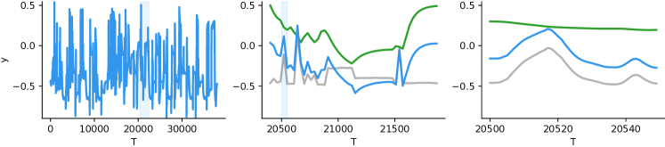
Figure 1: Resolution Matters. A semi-synthetic dataset (blue) created as a sum of two functions, one with fast varying dynamics (gray) and one with slowly varying dynamics (green)). Left: Shown is the complete trajectory. Using all observations for each parameter update is too time- and memory-consuming. Middle: Shown is a dilated mini-batch of size $50$ for which we have selected every $30$th observation. It allows for fitting the slowly varying function (green). The fast dynamics (gray) cannot be inferred as the observations are too sparse. Right: Shown is a mini-batch of size $50$ on the standard resolution. The mini-batch only covers a short interval of the trajectory as can be noted by the different time axis. It allows for fitting the fast varying function (gray). The slow dynamics (green) cannot be inferred as the gradient information is too weak. Our algorithm allows learning on multiple resolutions to capture effects on different timescales.

To address the problem of modeling long-term dependencies while retaining the computational advantage of mini-batching, we propose a novel GPSSM architecture with $L$ additive components. The resulting posterior is intractable, and we apply variational inference to find an efficient and structured approximation (blei2017variational). To capture effects on different time scales, our training scheme cycles through the components, whereby each component $l\in\{1,...,L\}$, is trained on a different resolution. For training the low-resolution components, we downsample the observations of the sequence, allowing us to pack a longer history in a mini-batch of fixed size (see Figure 1).

We further show that our algorithm is grounded in a coherent statistical framework by interpreting the GP transition model as a stochastic differential equation (SDE) similar to hegde2018deep. This relationship enables us to train our components on adaptive scales to capture effects on multiple time scales. From a numerical perspective, our method decomposes the dynamics of the data according to its required step sizes. Long-term effects are learned by low-resolution components corresponding to large step sizes, short-term effects by high-resolution components corresponding to small step sizes.

We validate our new algorithm experimentally and show that it works well in practice on semi-synthetic data and on a challenging engine modeling task. Furthermore, we demonstrate that our algorithm outperforms its competitors by a large margin in cases where the dataset consists of fast and slow dynamics. For the engine modeling task, we introduce a new dataset to the community that contains the raw emissions of a gasoline car engine and has over 500,000 measurements. The dataset is available at https://github.com/boschresearch/Bosch-Engine-Datasets.

2 Background on GPSSMs and SDEs

Gaussian Processes in a Nutshell

The GP prior, $f(x)\sim GP(0,k(x,x^{\prime}))$, defines a distribution over functions, $f:\mathbb{R}^{D_{x}}\rightarrow\mathbb{R}$, and is fully specified by the kernel $k:\mathbb{R}^{D_{x}}\times\mathbb{R}^{D_{x}}\rightarrow\mathbb{R}$. Given a set of arbitrary inputs, $x_{M}=\{x_{m}\}_{m=1}^{M}$, their function values, $f_{M}=\{f(x_{m})\}_{m=1}^{M}$, follow a Gaussian distribution $p(f_{M})=\mathcal{N}(f_{M}|0,\text{K}_{MM})$ where $\text{K}_{MM}=\{k(x_{m},x_{m^{\prime}})\}_{m=1,m^{\prime}=1}^{M}$.

For a new set of input points, $x_{N}=\{x_{n}\}_{n=1}^{N}$, the predictive distribution over the corresponding function values, $f_{N}=\{f(x_{n})\}_{n=1}^{N}$, can then be obtained by conditioning the joint distribution on $f_{M}$, leading to $p(f_{N}|f_{M})=\mathcal{N}(f_{N}|\mu(x_{N}),\Sigma(x_{N}))$ with

$$\mu(x_{N}) = \text{K}_{NM}\text{K}_{MM}^{-1}f_{M},$$ (1)

$$\Sigma(x_{N}) = \text{K}_{NN}-\text{K}_{NM}\text{K}_{MM}^{-1}\text{K}_{NM}^{\top},$$ (2)

where the cross-covariances $K_{NM}$ are defined similarly as $\text{K}_{MM}$, i.e. $\text{K}_{NM}=\{k(x_{n},x_{m})\}_{n,m=1}^{N,M}$. For a more detailed introduction, we refer the interested reader to rasmussen2006gaussian.

Gaussian Process State-Space Models

We are given a dataset $y_{T}=\{y_{t}\}_{t=1}^{T}$ over $T$ time points. Each time point $t$ is characterized by the outputs $y_{t}\in\mathbb{R}^{D_{y}}$. State-space models (see e.g. sarkka2013bayesian) offer a general way to describe time-series data by introducing a latent state, $x_{t}\in\mathbb{R}^{D_{x}}$, that captures the compressed history of the system, for each time point $t\in\{1,\ldots,T\}$. Assuming the process and observational noise to be i.i.d. Gaussian distributed, the model can be written down as follows:

$$x_{t+1}|x_{t}\sim\mathcal{N}(x_{t+1}|x_{t}+f(x_{t}),\text{Q}),\;\;\;\;\;\;\;\;\;\;y_{t}|x_{t}\sim\mathcal{N}(y_{t}|g(x_{t}),\Omega),$$

where $f:\mathbb{R}^{D_{x}}\rightarrow\mathbb{R}^{D_{x}}$ models the change of the latent state in time and $g:\mathbb{R}^{D_{x}}\rightarrow\mathbb{R}^{D_{y}}$ maps the latent state to the observational space. The covariance $\text{Q}\in\mathbb{R}^{{D_{x}}\times{D_{x}}}$ describes the process noise, and $\Omega\in\mathbb{R}^{{D_{y}}\times{D_{y}}}$ the observational noise. Following the literature (wang2005gaussian; deisenroth2011pilco), we assume that the update in the latent state can be modeled under a GP prior, i.e. $f(x)\sim GP(0,k(x,x^{\prime}))$. The model generalizes easily to problems with exogenous inputs that we left out in favor of an uncluttered notation.

Finally, we chose a linear model $g(x_{t})=Cx_{t}$ with output matrix $C\in\mathbb{R}^{D_{y}\times D_{x}}$ as emission function. This is a widely adopted design choice, since the linear emission model reduces non-identifiabilities of the solution (frigola2015bayesian). Our approach generalizes to non-linear models as well, which might for instance be important in cases in which prior knowledge supports the use of more expressive emission models.

Sparse Parametric Gaussian Process State-Space Models

Sparse GPs augment the model by a set of inducing points $(x_{M},f_{M})$ that can be exploited during inference to summarize the training data in an efficient way.  snelson2005sparse introduced the so-called FITC (fully independent training conditional) approximation on the augmented joint density $p(f_{M},f_{N})$ by assuming independence between the function values, $f_{N}$, conditioned on the set of inducing points, $f_{M}$, i.e. $p(f_{N},f_{M})\approx\prod_{n}p(f_{n}|f_{M})p(f_{M})$ with $p(f_{n}|f_{M})=\mathcal{N}(f_{n}|\mu(x_{n}),\Sigma(x_{n}))$. Recently, this and similar formulations have regained interest in the community, since they simplify inference and yield good empirical performance (jankowiak2020parametric; rossi2020rethinking). We follow this line of work by assuming the same conditional factorization,

$$f_{M} \sim\mathcal{N}(f_{M}|0,\text{K}_{MM}),$$ (3)

$$f_{t}|f_{M} \sim\mathcal{N}(f_{t}|\mu(x_{t}),\Sigma(x_{t})),$$ (4)

$$x_{t+1}|x_{t},f_{t} \sim\mathcal{N}(x_{t+1}|x_{t}+f_{t},\text{Q}),$$ (5)

where $f_{t}$ are the GP predictions at time index $t$ with mean $\mu(x_{t})$ and covariance $\Sigma(x_{t})$ [Eqs. eq:gpmean and eq:gpcov]. The FITC approximation has also found its way into the GPSSM literature: doerr2018probabilistic use it in the same way as we do (see also discussion in ialongo2019overcoming).

The difference to the standard formulation is mostly pronounced if we sample twice from the same region with large GP uncertainty [Eq. eq:gpcov]: samples from the FITC prior are assumed to be independent, while samples from the standard prior are correlated. Since the GP uncertainty is only large in input regions that are not covered by the inducing points, we deem the differences to be rather subtle and accept them in favor of establishing a bridge between the GPSSM and the GPSDE formulation, as we show in the following.

Gaussian Process Stochastic Differential Equations

SDEs can be regarded as a stochastic extension to ordinary differential equations where randomness enters the system via Brownian motion. Their connection to GPSSMs is obtained by considering the SDE