Distilled Domain Randomization

Abstract

Deep reinforcement learning is an effective tool to learn robot control policies from scratch. However, these methods are notorious for the enormous amount of required training data which is prohibitively expensive to collect on real robots. A highly popular alternative is to learn from simulations, allowing to generate the data much faster, safer, and cheaper. Since all simulators are mere models of reality, there are inevitable differences between the simulated and the real data, often referenced as the ‘reality gap’. To bridge this gap, many approaches learn one policy from a distribution over simulators. In this paper, we propose to combine reinforcement learning from randomized physics simulations with policy distillation. Our algorithm, called Distilled Domain Randomization (DiDoR), distills so-called teacher policies, which are experts on domains that have been sampled initially, into a student policy that is later deployed. This way, DiDoR learns controllers which transfer directly from simulation to reality, i.e., without requiring data from the target domain. We compare DiDoR against three baselines in three sim-to-sim as well as two sim-to-real experiments. Our results show that the target domain performance of policies trained with DiDoR is en par or better than the baselines’. Moreover, our approach neither increases the required memory capacity nor the time to compute an action, which may well be a point of failure for successfully deploying the learned controller.

I Introduction

Learning from randomized simulations has shown to be a promising approach for learning robot control policies that transfer to the real world. Examples cover manipulation [1, 2, 3, 4, 5], trajectory optimization [6], continuous control [7, 8, 9], vision [10, 11, 12, 13], and locomotion tasks [14, 15, 16]. Independent of the task, all domain randomization methods can be classified based on the fact if they use target domain data to update the distribution over simulators or not. While adapting the domain parameter distribution is in general superior, there are problem settings where (i) the target domain is not accessible until deployment, (ii) iterating a sim-to-real loop is too expensive, or (iii) the problem can be simulated well enough to directly execute the learned policy. For any of these three scenarios, zero-shot learning using domain randomization is either a viable or the only option. However, naive randomization approaches have the disadvantage that the domain parameter distribution is easily selected too wide, such that the agent can not learn something meaningful. In this case, the cause of failure is the large variance of the policy update, which results from collecting training data in many different environments at every update step. To resolve this issue, we propose to learn individual expert policies each mastering exactly one domain which has been sampled randomly from the distribution over simulators. Subsequently, these experts are used as teachers from which a student can learn by imitation. Here, we focus on the supervised learning technique called on-policy distillation [17, 18, 19, 20] which belongs to the overarching category of knowledge distillation [21] methods. Policy distillation transfers the behavior of one or more teacher policies, typically deep neural networks, into one (smaller) student policy. There are several other ways to learn from an ensemble of teachers [22], which are out of the scope of this paper.

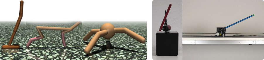
Figure 1: The evaluation platforms. Sim-to-sim (left): hopper, half-cheetah, and ant. Sim-to-real (right): Furuta pendulum, and cart-pole.

Contributions

We advance the state of the art by introducing Distilled Domain Randomization (DiDoR), the first algorithm which leverages the synergies between domain randomization and policy distillation to bridge the reality gap in robotics. Three particular synergies are: (i) The individual training procedures are more stable and reproducible compared to other domain randomization approaches, because the reinforcement learning for the teachers is done for one simulation instance only. (ii) For DiDoR, the computer only needs to hold one policy in memory at a time. (iii) Since the final network is small, the time to compute the next command is reduced significantly compared to methods that query an ensemble of experts. Especially the last two points are beneficial to satisfy real-time requirements on a physical device. Furthermore, DiDoR is easy to implement and parallelize, yet effective as demonstrated by comparing against three baselines in three sim-to-sim and two sim-to-real experiments. Finally, we made all our implementations available open-source in a common software framework. This also includes Peer-to-Peer Distillation Reinforcement Learning [23], which has not been tested in sim-to-real settings so far.

II Related Work

We categorize the related work by the two techniques that make up DiDoR: domain randomization (Section II-A), and policy distillation (Section II-B).

II-A Domain Randomization

The core idea of domain randomization is to expose the agent to various instances of the same environment such that it learns a policy which solves the task for a distribution of domain parameters, and therefore is more robust against model mismatch. Here, we focus on static domain randomization as used in DiDoR. These approaches do not update the domain parameter distribution, and directly deploy the learned policy in the target domain. More specifically, we narrow our selection down to algorithms that randomize the system dynamics and achieved the sim-to-real transfer.

Most prominently, the robotic in-hand manipulation reported by OpenAI in [1] demonstrated that domain randomization in combination with model engineering and the usage of recurrent neural networks enables direct sim-to-real transfer on an unprecedented difficulty level. Similarly, Peng et al. [2] combined model-free RL with recurrent neural network policies trained using experience replay in order to push an object by controlling a robotic arm. In contrast, Mordatch et al. [6] employed finite model ensembles to run trajectory optimization on a small-scale humanoid robot. After carefully identifying the system’s parameters, Lowrey et al. [3] learned a continuous controller for a three-finger positioning task. Their results show that the policy learned from the identified model was able to perform the sim-to-real transfer, but the policies learned from an ensemble of models were more robust to modeling errors. Tan et al. [14] presented an example for learning quadruped gaits from randomized simulations. They found empirically that sampling domain parameters from a uniform distribution together with applying random forces and regularizing the observation space can be sufficient to cross the reality gap. Aside from to the previous methods, Muratore et al. [8] introduce an approach to estimate the transferability of a policy learned from randomized physics simulations. Moreover, the authors propose a meta-algorithm which provides a probabilistic guarantee on the performance loss when transferring the policy between two domains form the same distribution.

II-B Policy Distillation

Policy distillation describes the transfer of knowledge about a specific task from one or multiple teachers to a student. This technique originates from the seminal work of Hinton et al. [21] which introduced knowledge distillation. The supervised learning method distills an ensemble of models into a single model, which typically is smaller than the original ones. Therefore, knowledge distillation can be seen as a generalization of model compression. In the context of (deep) RL, the knowledge transfer is achieved by training the student to imitate the teacher such that the decision making of the policy matches. While most of the related work considered deep Q-networks, knowledge distillation can be applied regardless of the model’s architecture or the method used for training the teachers. To the best of our knowledge, policy distillation was not applied in a sim-to-real scenario, yet.

Policy distillation is strongly connected to multi-task learning where each teacher is specialized in a different task, e.g. an Atari game [18, 24], or an image classifier [25]. In the multi-task setting, the teachers’ knowledge is distilled into a student in order to bootstrap the student’s learning procedure. Note that the approach presented in this paper has a fundamentally different goal. DiDoR distills multiple experts of the same task, but specialized in different instances, to obtain a control policy that is robust to model mismatch. Romero et al. [26] showed that besides model compression, policy distillation can yield students which improve over their teachers’ performance by choosing deeper and thinner neural networks for the student together with reusing the teachers’ hidden layers. Recently, Zhao et al. [23] proposed an online peer-to-peer distillation called Peer-to-Peer Distillation Reinforcement Learning (P2PDRL) which differs from previous methods during the distillation step. In line with the idea of domain randomization, each teacher is assigned to a random domain and the policy update is regularized by its peers. The regularization reduces the variance of the policy update. Unlike DiDoR, the teachers are assigned to a new domain at every iteration of the algorithm, which makes the training of the domain experts more noisy for P2PDRL. Moreover, P2PDRL requires all teachers to be held in memory during training. The authors evaluated P2PDRL on five sim-to-sim experiments using the MuJoCo physics engine. Czarnecki et al. [20] provided a unifying overview of policy distillation. According to their categorization, DiDoR can be labeled an on-policy distillation method. The authors emphasize that seemingly minor differences between the approaches can have major effects on the resulting algorithm, such as the loss of its convergence guarantees, or a different application scenario.

III Problem Statement and Notation

Consider a discrete-time dynamical system

$$\begin{gathered}\fs_{t+1}\sim\mathcal{P}_{\bm{\xi}}\!\left(\fs_{t+1}|\fs_{t},\fa_{t}\right),\quad\fs_{0}\sim\mu_{\bm{\xi}}\!\left(\fs_{0}\right),\\ \fa_{t}\sim\pi_{\ftheta}\!\left(\fa_{t}|\fs_{t}\right),\quad\bm{\xi}\sim p_{\bm{\phi}}\!\left(\bm{\xi}\right),\end{gathered}$$ (1)

with the continuous state ${\fs_{t}\in\mathcal{S}_{\bm{\xi}}\subseteq\mathbb{R}^{{n_{s}}}}$ and continuous action ${\fa_{t}\in\mathcal{A}_{\bm{\xi}}\subseteq\mathbb{R}^{{n_{a}}}}$ at a time step $t$. The environment, also called domain, is characterized by its parameters ${\bm{\xi}\in\mathbb{R}^{{n_{\xi}}}}$ (e.g., masses, friction coefficients, time delays, or camera properties) which are in general assumed to be random variables distributed according to an unknown probability distribution ${p\colon\mathbb{R}^{{n_{\xi}}}\to\mathbb{R}^{+}}$. Here we make the common assumption that the domain parameters or the true system obey a parametric distribution $p_{\bm{\phi}}\!\left(\bm{\xi}\right)$ with unknown parameters $\bm{\phi}$ (e.g., mean and variance). The domain parameters determine the transition probability density function ${\mathcal{P}_{\bm{\xi}}\colon\mathcal{S}_{\bm{\xi}}\times\mathcal{A}_{\bm{\xi}}\times\mathcal{S}_{\bm{\xi}}\to\mathbb{R}^{+}}$ that describes the system’s stochastic dynamics. The initial state $\fs_{0}$ is drawn from the start state distribution ${\mu_{\bm{\xi}}\colon\mathcal{S}_{\bm{\xi}}\to\mathbb{R}^{+}}$. We model the reward to be a deterministic function of the current state and action ${r_{\bm{\xi}}\colon\mathcal{S}_{\bm{\xi}}\times\mathcal{A}_{\bm{\xi}}\to\mathbb{R}}$. Together with the temporal discount factor ${\gamma\in[0,1]}$, the system forms a Markov Decision Process (MDP) described by the tuple ${\mathcal{M}_{\bm{\xi}}=\left\langle\mathcal{S}_{\bm{\xi}},\mathcal{A}_{\bm{\xi}},\mathcal{P}_{\bm{\xi}},\mu_{\bm{\xi}},r_{\bm{\xi}},\gamma\right\rangle}$.

The goal of a Reinforcement Learning (RL) agent is to maximize the expected (discounted) return, a numeric scoring function which measures the policy’s performance. The expected discounted return of a policy $\pi_{\ftheta}\!\left(\fa_{t}|\fs_{t}\right)$ with the parameters $\ftheta\in\Theta\subseteq\mathbb{R}^{{n_{\theta}}}$ is defined as

$$J\!\left(\ftheta,\bm{\xi}\right)= \mathbb{E}_{\fs_{0}\sim\mu_{\bm{\xi}}\left(\fs_{0}\right)}\bigg{[}\mathbb{E}_{\fs_{t+1}\sim\mathcal{P}_{\bm{\xi}}\left(\fs_{t},\fa_{t}\right),\ \fa_{t}\sim\pi_{\ftheta}\!\left(\fa_{t}|\fs_{t}\right)}\bigg{[}$$

$$\sum\nolimits_{t=0}^{T-1}\gamma^{t}r_{\bm{\xi}}\!\left(\fs_{t},\fa_{t}\right)\Big{|}\ftheta,\bm{\xi},\fs_{0}\bigg{]}\bigg{]}.$$ (2)

While learning from experience, the agent adapts its policy parameters. The resulting state-action-reward tuples are collected in trajectories, a.k.a. rollouts, ${\bm{\tau}=\{\fs_{t},\fa_{t},r_{t}\}_{t=0}^{T-1}\in\mathcal{T}}$ with $r_{t}=r_{\bm{\xi}}\!\left(\fs_{t},\fa_{t}\right)$. When augmenting the RL setting with domain randomization, the goal becomes to maximize the expected (discounted) return for a distribution of domain parameters

$$J\!\left(\ftheta\right) =\mathbb{E}_{\bm{\xi}\sim p\left(\bm{\xi}\right)}\!\left[J\!\left(\ftheta,\bm{\xi}\right)\right]$$ (3)

$$=\mathbb{E}_{\bm{\xi}\sim p\left(\bm{\xi}\right)}\!\left[\mathbb{E}_{\bm{\tau}\sim p(\bm{\tau})}\!\left[\sum\nolimits_{t=0}^{T-1}\gamma^{t}r_{\bm{\xi}}\!\left(\fs_{t},\fa_{t}\right)\Big{|}\ftheta,\bm{\xi},\fs_{0}\right]\right].$$

The outer expectation with respect to the domain parameter distribution $p\!\left(\bm{\xi}\right)$ is the key difference compared to the standard MDP formulation. It enables the learning of robust policies, in the sense that these policies work for a whole set of environments instead of overfitting to a particular instance.

IV Distilled Domain Randomization (DiDoR)

The goal of DiDoR is to learn a control policy in simulation such that it directly transfers to the real device, i.e., without using any data from the target domain. To accomplish this, DiDoR combines domain randomization with policy distillation. In the following, we describe the procedure in detail. A brief summary is given by Algorithm 1.

Figure 2: Sketch of the proposed sim-to-real method DiDoR.

input : domain parameter distribution $p_{\bm{\phi}}\!\left(\bm{\xi}\right)$, number of teachers $N$, iterations $I$, and epochs $E$

output : trained student policy parameters $\ftheta^{s}$

1 Initialize the teacher $\ftheta_{1:N}^{t}$ and the student $\ftheta^{s}$ policy parameters randomly

2 Sample one environment instance per teacher $\bm{\xi}_{1:N}\sim p_{\bm{\phi}}\!\left(\bm{\xi}\right)$

Train the teachers individually on their environment $\ftheta_{1:N}^{t}\leftarrow\textsc{PolOpt}(\bm{\xi}_{1:N})$

  $\triangleright$ parallelizable

3 for each iteration $i=1\!:\!I$ do

4       for each teacher $n=1\!:\!N$ do $\triangleright$ parallelizable

5             Execute student in each teacher domain $\ftau_{n}\leftarrow\textsc{Rollout}(\pi_{\ftheta^{s}},\bm{\xi}_{n})$ $\triangleright$ data collection

6      for each epoch $e=1\!:\!E$ do $\triangleright$ policy distillation

7             Compute the policy distillation loss $\mathcal{L}\leftarrow\sum_{n=1}^{N}\mathrm{KL}(\pi_{\ftheta_{n}^{t}}\!\left(\ftau_{n}\right)\|\pi_{\ftheta^{s}}\!\left(\ftau_{n}\right))$

8             Update $\ftheta^{s}$ using $\mathcal{L}_{\textrm{KL}}$

9            

Algorithm 1 Distilled Domain Randomization

First, we randomly initialize a set of $N$ teacher policies $\ftheta_{1:N}^{t}$ as well as the student policy $\ftheta^{s}$. For each teacher, one domain parameter configuration is sampled from the given domain parameter distribution $p_{\bm{\phi}}\!\left(\bm{\xi}\right)$. The parameters of this distribution are defined a priori by the user. Next, each teacher is trained exclusively in one of the sampled domains (Figure 2). There are no restrictions for the selection of the training algorithm or the policy type. At this point, we could utilize ensemble methods to create a policy out of the teacher networks, e.g., by averaging their actions. However, the time to compute a motor command linearly increases the number of teachers. Acting in the physical world, robots are subject to hard real-time constraints, which can severely limit ensemble-based methods (Section V-B). By distilling all teachers into one student, we obtain a single policy that encodes knowledge from all teachers. Therefore policy distillation approaches like DiDoR have a smaller memory footprint and faster execution times compared to ensemble methods. To gather the training data for distillation, we execute the student policy in every teacher environment, and collect the rollouts $\ftau_{1:N}$. Subsequently, we minimize the sum of Kullback-Leibler (KL) divergences between the action distributions of every student-teacher pair, given the collected rollouts:

$$\mathcal{L}=\sum\nolimits_{n=1}^{N}\mathrm{KL}\!\left(\pi_{\ftheta_{n}^{t}}\!\left(\ftau_{n}\right)\Big{\|}\pi_{\ftheta^{s}}\!\left(\ftau_{n}\right)\right)$$

This loss corresponds to a multi-teacher variant of on-policy distill [20] without the entropy penalty. We found the entropy penalty to be unnecessary in the sim-to-real setting, since the entropy of the resulting student policy is already regulated by the fact that the teacher policies have been learned using domain randomization. Hence, designing the domain parameter distribution $p_{\bm{\phi}}\!\left(\bm{\xi}\right)$ indirectly controls the entropy of the teacher policies.

V Experiments

To examine the robustness of DiDoR, we conducted three sim-to-sim (Section V-A) as well as two sim-to-real experiments (Section V-B). The sim-to-sim scenarios can be seen as a proof of concept, where we evaluate the learned policies in 32 unknown simulation instances randomly sampled from the domain parameter distribution. The sim-to-real experiments are significantly more challenging due to the underactuated nature of the chosen tasks as well as the inevitable approximation errors of the simulator. Moreover, robot control imposes hard time constraints. Since the control cycles of the cart-pole and the Furuta pendulum (Figure 1) are running at $500\text{\,}\mathrm{Hz}\text{/}$, the policy must not take more that $2\text{\,}\mathrm{ms}\text{/}$ to compute one forward pass. For simulating the randomized dynamical systems, we use the MuJoCo physics engine [27] as well as the SimuRLacra framework [28].

We compare DiDoR to the following baseline methods:

1. Uniform Domain Randomization (UDR) randomly samples a new set of domain parameters at every iteration, and updates the policy based on the data generated using these parameters. Thus, the policy permanently experiences new instances of the domain, which in turn leads to an increased robustness against model mismatch.

2. Ensemble Methods combine a set of policies in order to obtain a stronger model. Since we trained several teachers for DiDoR on different (random) domain instances, we can use them for the formation of an ensemble. However, there are numerous ways to query them. Motivated by prior experiments, we chose to average the action outputs of all policies within the ensemble. Hence, this baseline serves as a straightforward ablation of DiDoR without the policy distillation step. A considerable disadvantage of ensemble methods is that the execution time scales linearly with the number of elements, since this method requires a forward pass through all teacher policies. Nevertheless, this effect can be mitigated by using parallelization.

3. Peer-to-Peer Distillation Reinforcement Learning (P2PDRL) [23] is a policy distillation method aiming at learning robust policies. Similar to DiDoR, several teachers, here called workers, are trained on different domains. However, while our teachers are trained independently, these workers are trained at the same time and share knowledge via a special distillation loss, which in the end aligns the action distributions of the policies. Moreover, the domain parameters of the environments of the workers are drawn each iteration, while in DiDoR they stay fixed.

The training method as well as the policy architecture can be chosen freely for all algorithms. We decided to use Proximal Policy Optimization (PPO) [29] and feedforward neural networks. To facilitate a fair comparison, we tried to train all methods with similar configurations, e.g., UDR got as many iterations as all teachers combined. However, there were practical limitations which made a fair comparison difficult. While the teachers in DiDoR can train independently, all workers in P2PDRL work simultaneously and need to be kept in memory at the same time. Therefore, we had to reduce the number of workers for P2PDRL, especially for the MuJoCo environments (Section V-A) to one fourth of the number of teachers in DiDoR. Moreover, we choose all hyper-parameters which are common for the selected approaches, e.g. the policy architecture, identically. A report all hyper-parameters for training can be found in Table I. Moreover, we list the domain parameter distributions from the sim-to-real experiments in the appendix. To accelerate the learning, we followed the recommendations from [30] for on-policy training, finding that many of the suggestions did not yield the desired effect. However, initializing the action distribution of the policy such that it had approximately zero mean, significantly increased the initial return, thus decreased the number of necessary iterations.

V-A Sim-to-Sim Experiments

For a first validation in simulation, we used three locomotion tasks from the OpenAI Gym [31]: hopper, half-cheetah, and ant. We augmented each MuJoCo environment with domain randomization. However, the domain parameters of the training domain have lower variance than those of the test domain, therefore we can evaluate the robustness of the transfer. The commonality of the rather mixed sim-to-sim results displayed in Figure 3 is that DiDoR performs en par or better than the baselines depending on which metric is applied (e.g., highest median or highest peak performance). From the fact that, except for UDR, every approach works on at least two out of the three tasks, we conclude that the high variance of the returns originates from too aggressive domain randomization, i.e., a too broad domain parameter distribution.

(a) Sim-to-sim results for the hopper task

(b) Sim-to-sim results for the ant task

(c) Sim-to-sim results for the half-cheetah task

Figure 3: Sim-to-sim performance of the proposed method (DiDoR) as well as the baselines in three simulation environments: (left) evaluation of DiDoR’s student policy in its teacher domains. (right) evaluation of all methods in randomly sampled domains which have not been seen during training. The results were obtained by evaluating four policies, trained from different random seeds, per algorithm, each executing 100 rollouts with different initial states on 32 unknown simulation instances. The white circles mark the median values.

V-B Sim-to-Real Experiments

We evaluate the chosen methods’ zero-shot sim-to-real transfer on two underactuated swing-up and balance tasks (Figure 1). The Furuta pendulum [32] is a rotary inverted pendulum with fast dynamics. Its relatively short pendulum arm makes the stabilization of the upper equilibrium difficult. The cart-pole is a cart-driven inverted pendulum on a rail. For this platform, the contact between the cart’s wheel (soft plastic) and the rail (metal) is particularly hard to model. We strongly believe that the simulation does not capture some of the highly nonlinear friction effects. This hypotheses is backed up by the results in Figure 4(b) (right), which show a higher variance, i.e., a higher failure rate, across all methods. In contrast, the middle subplots in Figure 4 reveal that all methods were able to solve both simulated swing-up and balance tasks. Comparing the left and middle subplots in Figure 4, we observe that DiDoR performed equally well on randomly sampled domains as on the teacher domains, providing evidence for good generalization capabilities. We explain the UDR policies’ inability to transfer by a too narrow domain parameter distribution. The most likely consequence of this is that UDR did not capture enough variation during training while still learning with its high-variance gradient estimates. The sim-to-real deployment on the Furuta pendulum is more benign (Figure 4(a)). Aside from negligibly few failures of two baseline methods, the vast majority of policies transferred.

During our experiments, we observed that at some points in time the individual elements of the ensemble baselines commanded actions which approximately canceled each other. If desired, this situation can be resolved by replacing the average over policy outputs with a different querying strategy. Finally, we attribute the relatively low performance of P2PDRL to a suboptimal hyper-parameter selection. Unfortunately, the suggestions in [23] did not produce satisfying results. This might be due to the fact that the authors tuned the parameters for other sim-to-sim tasks.

(a) Sim-to-real underactuated swing-up and balance task on the Furuta pendulum

(b) Sim-to-real underactuated swing-up and balance task on the cart-pole

Figure 4: Sim-to-real performance of the proposed method (DiDoR) as well as the baselines on two physical platforms: (left) evaluation of DiDoR’s student policy in its teacher domains. (middle) evaluation of all methods in randomly sampled domains which have not been seen during training. The results were obtained by evaluating four policies, trained from different random seeds, per algorithm, each executing 100 rollouts with different initial states on 32 simulation instances. The white circles mark the median values. (right) evaluation of all methods on the real-world device. The return was estimated from four policies per method, each executed 10 times on both platforms.

Table I: Hyper-parameters for training all reported policies.

Parameter	Value
algorithm	PPO [29] with GAE [33]
policy architecture	FNN 64-64 tanh
rollout length	8000 steps at $500\text{\,}\mathrm{Hz}\text{/}$
discount factor $\gamma$	0.99
lambda	0.97
parallel environments	48 (sim-to-real), 64 (sim-to-sim)
number of iterations	40
initial exploration variance	1.0
PPO clip ratio	0.1
learning rate	$110-3$ (sim-to-real), $110-4$ (sim-to-sim)
KL clip (PPO update)	0.05
DiDoR specific
teacher number	16 (sim-to-real), 8 (sim-to-sim)
P2PDRL specific
worker number	4 (cart-pole), 2 (all other tasks)
distillation loss coefficient $\alpha$	0.05 (sim-to-real), 0.01 (sim-to-sim)

VI Conclusion

We have introduced Distilled Domain Randomization (DiDoR), an algorithm that combines domain randomization and knowledge distillation to learn policies that are able to transfer from simulation to reality. By distilling the expert knowledge of multiple teachers, which have been learned in various instances of the problem, the resulting student policy is more robust to the inevitable model mismatch that occurs when deploying a learned policy on the physical system. We have evaluated the presented method on three sim-to-sim and two sim-to-real experiments. Our results show the advantages of DiDoR over uniform domain randomization, an ensemble of teachers, and Peer-to-Peer Distillation Reinforcement Learning. In contrast to these baselines, DiDoR neither increases the required memory capacity, nor the time to compute an action. Both features make the proposed approach better suited for high-frequency control on real robots. Moreover, DiDoR is vastly parallelizable and has been shown to generalize better to unseen domains. For future research, we plan to investigate the effect of replacing the distillation loss, as for example described in [20].

Appendix

In the subsequent tables, we list the domain parameter distributions of the Furuta pendulum (Table II) and the cart-pole (Table III) experiments. Normal distributions are parameterized with mean and standard deviation, uniform distributions with lower and upper bound.

Table II: The domain parameter distribution for the sim-to-real Furuta pendulum experiment.

Parameter	Distribution
gravity constant	$\mathcal{N}\left(g\big{|}$9.81$,$0.981$\right)$\mathrm{kg}\text{/}$$
pend. pole mass	$\mathcal{N}\left(m_{p}\big{|}$0.024$,$0.048$\right)$\mathrm{kg}\text{/}$$
rot. pole mass	$\mathcal{N}\left(m_{p}\big{|}$0.095$,$0.019$\right)$\mathrm{kg}\text{/}$$
pend. pole length	$\mathcal{N}\left(l_{p}\big{|}$0.129$,$0.026$\right)$\mathrm{m}\text{/}$$
rot. pole length	$\mathcal{N}\left(l_{r}\big{|}$0.085$,$0.017$\right)$\mathrm{m}\text{/}$$
pend. pole damping	$\mathcal{U}\left(d_{p}\big{|}$110-6$,$2.510-7$\right)$\mathrm{N}\text{\,}\mathrm{m}\text{\,}\mathrm{s}\text{/}\mathrm{rad}$$
rot. pole damping	$\mathcal{N}\left(d_{r}\big{|}$510-6$,$1.2510-6$\right)$\mathrm{N}\text{\,}\mathrm{m}\text{\,}\mathrm{s}\text{/}\mathrm{rad}$$
motor resistance	$\mathcal{N}\left(R_{m}\big{|}$8.4$,$1.68$\right)$\mathrm{\SIUnitSymbolOhm}\text{/}$$
motor constant	$\mathcal{N}\left(k_{m}\big{|}$0.042$,$8.410-3$\right)$\mathrm{N}\text{\,}\mathrm{m}\text{/}\mathrm{A}$$

Table III: The domain parameter distribution for the sim-to-real cart-pole experiment.

Parameter	Distribution
gravity constant	$\mathcal{N}\left(g\big{|}$9.81$,$0.981$\right)$\mathrm{kg}\text{/}$$
cart mass	$\mathcal{N}\left(m_{c}\big{|}$0.38$,$0.076$\right)$\mathrm{kg}\text{/}$$
pole mass	$\mathcal{N}\left(m_{p}\big{|}$0.127$,$2.5410-2$\right)$\mathrm{kg}\text{/}$$
pole length	$\mathcal{N}\left(l_{p}\big{|}$0.168\,25$,$3.36510-2$\right)$\mathrm{m}\text{/}$$
rail length	$\mathcal{N}\left(l_{r}\big{|}$0.814$,$0.163$\right)$\mathrm{m}\text{/}$$
motor pinion radius	$\mathcal{N}\left(r_{mp}\big{|}$6.3510-3$,$1.2710-3$\right)$\mathrm{m}\text{/}$$
gear ratio	$\mathcal{N}\left(K_{g}\big{|}3.71,0.93\right)$
gearbox efficiency	$\mathcal{U}\left(\eta_{g}\big{|}$0.675$,$1.0$\right)$
motor efficiency	$\mathcal{U}\left(\eta_{m}\big{|}$0.675$,$1.0$\right)$
motor moment of inertia	$\mathcal{N}\left(J_{m}\big{|}$3.910-7$,$9.7510-8$\right)$\mathrm{kg}\text{\,}{\mathrm{m}}^{2}\text{/}$$
motor torque constant	$\mathcal{N}\left(k_{m}\big{|}$7.6710-3$,$1.9210-3$\right)$\mathrm{N}\text{\,}\mathrm{m}\text{/}\mathrm{A}$$
motor armature resistance	$\mathcal{N}\left(R_{m}\big{|}$2.6$,$0.65$\right)$\mathrm{\SIUnitSymbolOhm}\text{/}$$
motor viscous damping coeff. w.r.t. load	$\mathcal{U}\left(B_{\textrm{eq}}\big{|}$4.05$,$6.75$\right)$\mathrm{N}\text{\,}\mathrm{s}\text{/}\mathrm{m}$$
pole viscous friction coeff.	$\mathcal{U}\left(B_{p}\big{|}$1.810-3$,$3.0$\right)$\mathrm{N}\text{\,}\mathrm{s}\text{/}$$
friction coefficient cart - rail	$\mathcal{U}\left(\mu_{c}\big{|}$0.01$,$0.03$\right)$

References

- [1] OpenAI, M. Andrychowicz, B. Baker, M. Chociej, R. Józefowicz, B. McGrew, J. W. Pachocki, A. Petron, M. Plappert, G. Powell, A. Ray, J. Schneider, S. Sidor, J. Tobin, P. Welinder, L. Weng, and W. Zaremba, “Learning dexterous in-hand manipulation,” Int. J. Robot. Res., vol. 39, no. 1, 2020. [Online]. Available: https://doi.org/10.1177/0278364919887447
- [2] X. B. Peng, M. Andrychowicz, W. Zaremba, and P. Abbeel, “Sim-to-real transfer of robotic control with dynamics randomization,” in ICRA, Brisbane, Australia, May 21-25, 2018, pp. 1–8. [Online]. Available: https://doi.org/10.1109/ICRA.2018.8460528
- [3] K. Lowrey, S. Kolev, J. Dao, A. Rajeswaran, and E. Todorov, “Reinforcement learning for non-prehensile manipulation: Transfer from simulation to physical system,” in SIMPAR 2018, Brisbane, Australia, May 16-19, 2018, pp. 35–42. [Online]. Available: https://doi.org/10.1109/SIMPAR.2018.8376268
- [4] OpenAI, I. Akkaya, M. Andrychowicz, M. Chociej, M. Litwin, B. McGrew, A. Petron, A. Paino, M. Plappert, G. Powell, R. Ribas, J. Schneider, N. Tezak, J. Tworek, P. Welinder, L. Weng, Q. Yuan, W. Zaremba, and L. Zhang, “Solving rubik’s cube with a robot hand,” ArXiv e-prints, vol. 1910.07113, 2019. [Online]. Available: http://arxiv.org/abs/1910.07113
- [5] Y. Chebotar, A. Handa, V. Makoviychuk, M. Macklin, J. Issac, N. D. Ratliff, and D. Fox, “Closing the sim-to-real loop: Adapting simulation randomization with real world experience,” in ICRA, Montreal, QC, Canada, May 20-24, 2019, pp. 8973–8979. [Online]. Available: https://doi.org/10.1109/ICRA.2019.8793789
- [6] I. Mordatch, K. Lowrey, and E. Todorov, “Ensemble-cio: Full-body dynamic motion planning that transfers to physical humanoids,” in IROS, Hamburg, Germany, September 28 - October 2, 2015, pp. 5307–5314. [Online]. Available: https://doi.org/10.1109/IROS.2015.7354126
- [7] W. Yu, J. Tan, C. K. Liu, and G. Turk, “Preparing for the unknown: Learning a universal policy with online system identification,” in RSS, Cambridge, Massachusetts, USA, July 12-16, 2017. [Online]. Available: http://www.roboticsproceedings.org/rss13/p48.html
- [8] F. Muratore, M. Gienger, and J. Peters, “Assessing transferability from simulation to reality for reinforcement learning,” IEEE Trans. Pattern Anal. Mach. Intell., vol. 43, pp. 1172–1183, 11 2021. [Online]. Available: https://doi.org/10.1109/TPAMI.2019.2952353
- [9] F. Muratore, C. Eilers, M. Gienger, and J. Peters, “Data-efficient domain randomization with bayesian optimization,” IEEE Robotics Autom. Lett., vol. 6, no. 2, pp. 911–918, 2021. [Online]. Available: https://doi.org/10.1109/LRA.2021.3052391
- [10] J. Tobin, R. Fong, A. Ray, J. Schneider, W. Zaremba, and P. Abbeel, “Domain randomization for transferring deep neural networks from simulation to the real world,” in IROS, Vancouver, BC, Canada, September 24-28, 2017, pp. 23–30. [Online]. Available: https://doi.org/10.1109/IROS.2017.8202133
- [11] F. Sadeghi and S. Levine, “CAD2RL: real single-image flight without a single real image,” in RSS, Cambridge, Massachusetts, USA, July 12-16, 2017. [Online]. Available: http://www.roboticsproceedings.org/rss13/p34.html
- [12] J. Tobin, L. Biewald, R. Duan, M. Andrychowicz, A. Handa, V. Kumar, B. McGrew, A. Ray, J. Schneider, P. Welinder, W. Zaremba, and P. Abbeel, “Domain randomization and generative models for robotic grasping,” in IROS, Madrid, Spain, October 1-5, 2018, pp. 3482–3489. [Online]. Available: https://doi.org/10.1109/IROS.2018.8593933
- [13] S. James, P. Wohlhart, M. Kalakrishnan, D. Kalashnikov, A. Irpan, J. Ibarz, S. Levine, R. Hadsell, and K. Bousmalis, “Sim-to-real via sim-to-sim: Data-efficient robotic grasping via randomized-to-canonical adaptation networks,” in CVPR, Long Beach, CA, USA, June 16-20. Computer Vision Foundation / IEEE, 2019, pp. 12 627–12 637.
- [14] J. Tan, T. Zhang, E. Coumans, A. Iscen, Y. Bai, D. Hafner, S. Bohez, and V. Vanhoucke, “Sim-to-real: Learning agile locomotion for quadruped robots,” in RSS, Pittsburgh, Pennsylvania, USA, June 26-30, 2018. [Online]. Available: http://www.roboticsproceedings.org/rss14/p10.html
- [15] R. Antonova, A. Rai, T. Li, and D. Kragic, “Bayesian optimization in variational latent spaces with dynamic compression,” in CoRL, Osaka, Japan, October 30 - November 1, ser. Proceedings of Machine Learning Research, vol. 100. PMLR, 2019, pp. 456–465. [Online]. Available: http://proceedings.mlr.press/v100/antonova20a.html
- [16] X. B. Peng, E. Coumans, T. Zhang, T. E. Lee, J. Tan, and S. Levine, “Learning agile robotic locomotion skills by imitating animals,” in RSS, Virtual Event / Corvalis, Oregon, USA, July 12-16, 2020. [Online]. Available: https://doi.org/10.15607/RSS.2020.XVI.064
- [17] S. Ross, G. J. Gordon, and D. Bagnell, “A reduction of imitation learning and structured prediction to no-regret online learning,” in AISTATS, Fort Lauderdale, USA, April 11-13, ser. JMLR Proceedings, vol. 15. JMLR.org, 2011, pp. 627–635. [Online]. Available: http://proceedings.mlr.press/v15/ross11a/ross11a.pdf
- [18] E. Parisotto, L. J. Ba, and R. Salakhutdinov, “Actor-mimic: Deep multitask and transfer reinforcement learning,” in ICLR, San Juan, Puerto Rico, May 2-4, 2016. [Online]. Available: http://arxiv.org/abs/1511.06342
- [19] K. Lin, S. Wang, and J. Zhou, “Collaborative deep reinforcement learning,” ArXiv e-prints, vol. 1702.05796, 2017. [Online]. Available: http://arxiv.org/abs/1702.05796
- [20] W. M. Czarnecki, R. Pascanu, S. Osindero, S. M. Jayakumar, G. Swirszcz, and M. Jaderberg, “Distilling policy distillation,” in AISTATS, Naha, Okinawa, Japan, 16-18 April, ser. Proceedings of Machine Learning Research, vol. 89. PMLR, 2019, pp. 1331–1340. [Online]. Available: http://proceedings.mlr.press/v89/czarnecki19a.html
- [21] G. Hinton, O. Vinyals, and J. Dean, “Distilling the Knowledge in a Neural Network,” ArXiv e-prints, 2015, arXiv: 1503.02531. [Online]. Available: http://arxiv.org/abs/1503.02531
- [22] T. Osa, J. Pajarinen, G. Neumann, J. A. Bagnell, P. Abbeel, and J. Peters, “An algorithmic perspective on imitation learning,” Found. Trends Robotics, vol. 7, no. 1-2, pp. 1–179, 2018. [Online]. Available: https://doi.org/10.1561/2300000053
- [23] C. Zhao and T. M. Hospedales, “Robust domain randomised reinforcement learning through peer-to-peer distillation,” ArXiv e-prints, vol. 2012.04839, 2020. [Online]. Available: https://arxiv.org/abs/2012.04839
- [24] A. A. Rusu, S. G. Colmenarejo, Ç. Gülçehre, G. Desjardins, J. Kirkpatrick, R. Pascanu, V. Mnih, K. Kavukcuoglu, and R. Hadsell, “Policy distillation,” in ICLR, San Juan, Puerto Rico, May 2-4, 2016. [Online]. Available: http://arxiv.org/abs/1511.06295
- [25] W.-H. Li and H. Bilen, “Knowledge distillation for multi-task learning,” in Computer Vision – ECCV 2020 Workshops. Springer, 2020, pp. 163–176.
- [26] A. Romero, N. Ballas, S. E. Kahou, A. Chassang, C. Gatta, and Y. Bengio, “Fitnets: Hints for thin deep nets,” in ICLR, San Diego, CA, USA, May 7-9, 2015. [Online]. Available: http://arxiv.org/abs/1412.6550
- [27] E. Todorov, T. Erez, and Y. Tassa, “Mujoco: A physics engine for model-based control,” in IROS, Vilamoura, Algarve, Portugal, October 7-12, 2012, pp. 5026–5033. [Online]. Available: https://doi.org/10.1109/IROS.2012.6386109
- [28] F. Muratore, “Simurlacra - a framework for reinforcement learning from randomized simulations,” https://github.com/famura/SimuRLacra, 2020.
- [29] J. Schulman, F. Wolski, P. Dhariwal, A. Radford, and O. Klimov, “Proximal policy optimization algorithms,” ArXiv e-prints, 2017. [Online]. Available: http://arxiv.org/abs/1707.06347
- [30] M. Andrychowicz, A. Raichuk, P. Stanczyk, M. Orsini, S. Girgin, R. Marinier, L. Hussenot, M. Geist, O. Pietquin, M. Michalski, S. Gelly, and O. Bachem, “What matters in on-policy reinforcement learning? a large-scale empirical study,” ArXiv e-prints, vol. 2006.05990, 2020. [Online]. Available: https://arxiv.org/abs/2006.05990
- [31] G. Brockman, V. Cheung, L. Pettersson, J. Schneider, J. Schulman, J. Tang, and W. Zaremba, “Openai gym,” 2016. [Online]. Available: http://arxiv.org/abs/1606.01540
- [32] K. Furuta, M. Yamakita, and S. Kobayashi, “Swing-up control of inverted pendulum using pseudo-state feedback,” Proc. Inst. Mech. Eng. Part I, vol. 206, no. 4, pp. 263–269, 1992.
- [33] J. Schulman, P. Moritz, S. Levine, M. I. Jordan, and P. Abbeel, “High-dimensional continuous control using generalized advantage estimation,” ArXiv e-prints, vol. 1506.02438, 2015. [Online]. Available: http://arxiv.org/abs/1506.02438