Sidestepping the inversion of the weak-lensing covariance matrix with Approximate Bayesian Computation

Abstract

Weak gravitational lensing is one of the few direct methods to map the dark-matter distribution on large scales in the Universe, and to estimate cosmological parameters. We study a Bayesian inference problem where the data covariance $\bm{\mathrm{C}}$, estimated from a number $n_{\textrm{s}}$ of numerical simulations, is singular. In a cosmological context of large-scale structure observations, the creation of a large number of such $N$-body simulations is often prohibitively expensive. Inference based on a likelihood function often includes a precision matrix, $\Psi=\bm{\mathrm{C}}^{-1}$. The covariance matrix corresponding to a $p$-dimensional data vector is singular for $p\geq n_{\textrm{s}}$, in which case the precision matrix is unavailable. We propose the likelihood-free inference method Approximate Bayesian Computation (ABC) as a solution that circumvents the inversion of the singular covariance matrix. We present examples of increasing degree of complexity, culminating in a realistic cosmological scenario of the determination of the weak-gravitational lensing power spectrum for the upcoming European Space Agency satellite Euclid. While we found the ABC parameter estimate variances to be mildly larger compared to likelihood-based approaches, which are restricted to settings with $p<n_{\textrm{s}}$, we obtain unbiased parameter estimates with ABC even in extreme cases where $p/n_{\textrm{s}}\gg 1$. The code has been made publicly available to ensure the reproducibility of the results.

figurec

[A] addressline=AIM, CEA, CNRS, Université Paris-Saclay, Université de Paris, city=Gif-sur-Yvette, postcode=91191, country=France

[B] addressline=Université Clermont Auvergne, CNRS/IN2P3, LPC, postcode=63000, city=Clermont-Ferrand, country=France

[C] addressline=Department of Statistics, University of Wisconsin, city=Madison, postcode=53706, country=USA

1 Introduction

Matter on large scales in our Universe is distributed in structures such as walls, filaments, and halos that form the so-called cosmic web [e.g., 76, 34], and most of the matter is composed of dark matter. A powerful probe to measure statistical properties of the cosmic (dark-)matter density is weak gravitational lensing, which is the phenomenon of light rays being deflected by the tidal gravitational fields of the large-scale structure (LSS). These deflections result in the images of observed galaxies being distorted coherently, which is referred to as cosmic shear. The measurement of galaxy shapes and their correlations allow us to infer certain statistical and time-varying properties of the LSS, and the geometry of the Universe.

Cosmological inference attempts to determine the parameters of the cosmological model that describes the LSS and geometry of the Universe at different epochs using observed galaxies at a range of distances from us. Weak lensing is most sensitive to two cosmological parameters: (i) the matter density parameter $\Omega_{\textrm{m}}$, which is the present-day ratio of the matter density, $\rho_{\mathrm{m}}$, and critical density, $\rho_{\mathrm{crit}}=3H_{0}^{2}/(8\pi G)$, where $H_{0}=100\,h$ km s^-1 Mpc^-1 is the Hubble constant and $G$ is Newton’s gravitational constant; (ii) $\sigma_{8}$, the standard deviation of density fluctuations in spheres of $8h^{-1}$ Mpc radius. The parameter $\sigma_{8}$ is also the normalisation of the density power spectrum, which we introduce later.

One of the main weak-lensing observables is the angular power spectrum of cosmic shear, $C_{\ell}$, which measures shear correlations induced by the LSS as a function of angular Fourier mode on the sky, denoted by $\ell$. A mode $\ell$ denotes a spatial frequency on the sphere, which is related to angular distance on the sky $\vartheta$ as $\vartheta=\pi/\ell$. Due to the non-linear and non-Gaussian evolution of the cosmic matter density field, different scales become correlated. For weak-lensing inference of cosmological parameters, these correlations need to be included to avoid biasing the estimated parameters and their uncertainties [4, 67], which is accomplished by estimating the covariance of the lensing observables [39, 63].

Despite the non-Gaussian nature of the observables, a multivariate normal distribution for the likelihood is a good approximation in many cases [e.g., 68, 22]. This is because the intrinsically non-Gaussian shear is estimated by measuring galaxy shapes where the corresponding noise contribution is due to the variability of the intrinsic shape of galaxies, which is uncorrelated and Gaussian. This noise is particularly important on small and intermediate scales, where the intrinsic shear field is non-Gaussian. This renders the distribution of observed shear more Gaussian, and biases on cosmological parameter from inference under a multivariate normal likelihood approximation are small [49].

A multivariate normal distribution depends on the data covariance matrix $\bm{\mathrm{C}}$. To obtain this matrix for high-dimensional and correlated data is challenging. Several options have been pursued for cosmic shear. One option is based on analytical calculation using a model prediction [40]. This typically involves higher-order statistics for which models are not well known. Moreover, astrophysical and observational systematic effects such as intrinsic galaxy alignment for weak lensing [33] are difficult to model. Another approach is estimation from the data [20], which requires a sufficiently large data volume to create sub-samples. In addition, estimators such as Jackknife re-sampling are likely to provide results with an unacceptable bias. A third approach uses numerical simulations of the data, such as $N$-body simulations [25]. These are typically very expensive so that only a relatively small number $n_{\textrm{s}}$ of independent simulations are available for a restricted number of cosmological models.

An additional difficulty comes from the fact that evaluating the likelihood function requires the inverse of the covariance $\bm{\mathrm{C}}$ (i.e., the precision matrix $\bm{\mathrm{\Psi}}$). Since matrix inversion is a highly non-linear operation, uncertainties in the elements of $\bm{\mathrm{C}}$ are amplified and spread throughout $\bm{\mathrm{\Psi}}$. This mixing of matrix elements can create undesired correlations. In a cosmological context this can correlate errors on different scales, which could be the case if simulations are unreliable or biased on certain scales. For example, dark-matter-only $N$-body simulations are biased on small scales due to the lack of baryonic physics in those simulations [13]. In this paper we focus on the simulation-based estimation of the covariance matrix. The precision and accuracy of the estimated precision matrix, $\hat{\bm{\mathrm{\Psi}}}$, depend on the ratio $p/n_{\rm s}$, where $p$ is the dimension of the data (in our setting, this is the number of $\ell$-modes on which the cosmic-shear power spectrum is measured), and the number of available simulations $n_{\rm s}$. The smaller $p/n_{\rm s}$ is, the more precise the matrix estimation. If $p/n_{\rm s}\geq 1$, the estimated covariance matrix is singular, and the precision matrix is undefined [55]. Even if $p/n_{\rm s}<1$ the estimated $\hat{\bm{\mathrm{\Psi}}}$ suffers from a variance that depends on $p/n_{\rm s}$ and increases the uncertainty of the estimated parameters. To reach a desired high accuracy of the estimated parameters from likelihood inference, the ratio $p/n_{\rm s}$ has to be much smaller than unity [74].

Current cosmological observations from dedicated experiments or surveys provide data vectors used for inference with typical sizes of order $p\sim 100$. For future experiments such as the Vera Rubin Observatory (VRO) Legacy Survey of Space and Time [50] or the ESA space mission Euclid [17], this number can be thousands, or even tens of thousands when weak-lensing is combined with other cosmological probes. Keeping the $p/n_{\rm s}$ ratio low would therefore require a large number of $N$-body simulations of LSS, which includes modeling the mutual gravitational interaction of $N\sim{\cal O}(10^{9-11})$ mass points over cosmic times. Such simulations demand substantial computation time, memory, and storage space; hence, producing them in these large numbers for the estimation of $\bm{\mathrm{\Psi}}$ is extremely challenging.

To address these challenges, we develop an approach for inference with weak gravitational lensing using Approximate Bayesian Computation [ABC; e.g., 8, 6, 53] that does not require the estimation of the precision matrix, but only the covariance matrix. An important advantage of using ABC is that a likelihood function does not need to be specified, but instead a forward model is used to generate realizations that are then compared to the real observations. However, this does not preclude the use of a likelihood-motivated generative model. In the proposed method, the generative model is motivated by a Gaussian likelihood function, but with ABC an inverse covariance matrix is not needed. One of the key benefits of this approach is that it allows for the setting where $p/n_{\rm s}\geq 1$. For parameter inference with ABC we do not need to evaluate the likelihood function, $L$, but instead can produce random samples from the data-generating distribution; in our weak-lensing setting where assuming a multivariate normal distribution is considered reasonable, this only requires an estimate of $\bm{\mathrm{C}}$.

ABC has been explored in previous work for weak lensing for various observables such as weak-lensing peak counts [47, 48], which is the number of maxima in a (filtered) observed shear map. Peaks are a sensitive cosmological probe of non-Gaussian structures, since they trace the over-dense, highly non-linear regions in the cosmic density field. Further ABC studies were undertaken for the cosmic-shear power spectrum [37], and its Fourier transform, the correlation function [15].

While the focus of this paper is weak gravitational lensing, the methods developed are applicable to other settings where bypassing the direct estimation of the precision matrix is desirable. However, a way to simulate realizations of the data is needed.

In this paper we show empirically that our proposed ABC approach can provide unbiased parameter estimates and uncertainties that are relatively stable with respect to the number of simulations used for the covariance matrix estimation. We find that the number of simulations can be as low as $n_{\textrm{s}}=2$ and still produce reasonable estimates of $\bm{\mathrm{C}}$. As noted above, an incorrect precision matrix can bias likelihood-based inferred parameters, see also [67]. Such biases are amplified during the matrix inversion, and localised errors can spread across the entire matrix. Our approach minimizes such undesired effects, and we can expect a lower sensitivity of the inferred parameters to covariance matrix errors. We emphasize that we are using a likelihood-motivated forward model for the ABC algorithm; a different generative model could also be considered that does not require a covariance matrix, but may have other costs such as more computationally-intensive data generation.

The article is organised as follows. We provide a brief introduction to cosmological inference with weak gravitational lensing in Sect. 2 to motivate our approach. Section 3 gives an overview of our methodology using ABC. Section 4 discusses our three simulation studies that demonstrate the performance and limits of the proposed approach. These include a simple linear model (Sect. 4.2), a non-linear weak-lensing inspired function (Sect. 4.3), and a realistic weak-lensing case (Sect. 4.4). Concluding remarks are presented in Sect. 5.

2 Background

We begin this section by providing additional background on our motivating example of cosmological inference using weak lensing, including a description of the statistical model of the corresponding observable. Then we present some details about covariance and precision matrix estimation, which motivates our use of ABC.

2.1 Weak gravitational lensing

In most results from gravitational lensing observations to date, the data are second-order statistics of the weak-lensing cosmic shear field, and thus can be derived from the shear power spectrum $C_{\ell}$. The power spectrum is a one-dimensional function of angular Fourier scale $\ell$, which is the modulus of the 2D Fourier vector $\bm{\ell}$ on the sky.

2.1.1 The density contrast power spectrum

Before defining the weak-lensing power spectrum $C_{\ell}$, several other quantities need to be introduced. The density contrast, $\delta(\bm{x},z)=[\rho(\bm{x},z)-\bar{\rho}(z)]/\bar{\rho}(z)$, is the scaled matter density fluctuation $\rho$ around the spatial mean, $\bar{\rho}$, at redshift $z$, and 3D position $\bm{x}$. Redshift is the relative wavelength change between emitted and observed radiation of an object. In general, due to the expansion of the Universe the receding velocity of a galaxy increases with distance, which results in a larger redshift. Redshift can be used as a proxy for cosmological distance. The position vector $\bm{x}$ is a comoving coordinate, which remains constant with the expansion of the Universe. At early times and on large scales, $\left|\delta\right|\ll 1$, and the evolution of the density can be described by linear Newtonian perturbation theory [e.g., 56, 16]. On small scales, the non-linear evolution due to gravitational collapse is typically modeled by phenomenological approaches, e.g., parameterized models of halo formation and clustering, some based on numerical simulations [71].

The first moment of the density field vanishes by definition, $\mathbb{E}\left(\delta\right)=0$. Its second moment, or two-point correlation function $\xi_{\delta}$ is defined as

$$\xi_{\delta}(\bm{x}_{1},\bm{x}_{2})=\mathbb{E}\left[\delta(\bm{x}_{1})\delta(\bm{x}_{2})\right]=\int\int\delta(\bm{x}_{1})\delta(\bm{x}_{2})P[\delta(\bm{x}_{1}),\delta(\bm{x}_{2})]\mathrm{d}\delta(\bm{x}_{1})\mathrm{d}\delta(\bm{x}_{2}),$$ (1)

where $P[\delta(\bm{x}_{1}),\delta(\bm{x}_{2})]$ is the joint probability distribution function of $\delta(\bm{x}_{1})$ at position $\bm{x}_{1}$ and $\delta(\bm{x}_{2})$ at $\bm{x}_{2}$.

We assume that on large scales the density field is statistically homogeneous and isotropic. In that case, the two-point correlation function is invariant under translation and rotation such that $\xi_{\delta}(\bm{x}_{1},\bm{x}_{2})=\xi_{\delta}(|\bm{x}_{1}-\bm{x}_{2}|)$. In addition, the Fourier transform of $\xi_{\delta}$, known as the 3D power spectrum of the density field $P_{\delta}$, can be written as

$$P_{\delta}(k)=\int_{\mathbb{R}^{3}}\mathrm{d}^{3}y\,\mathrm{e}^{\mathrm{i}\bm{k}\bm{y}}\xi_{\delta}(y).$$ (2)

Due to statistical isotropy the power spectrum only depends on the modulus of the 3D wave mode, $k=|\bm{k}|$.

2.1.2 The weak-lensing power spectrum

For weak gravitational lensing by galaxies, the basic observable is the shape of a galaxy, expressed as complex ellipticity $\varepsilon$. Lensing by the LSS changes the galaxy shape, and imprints a shear $\gamma$. If a galaxy has an intrinsic ellipticity $\varepsilon^{\rm s}$, to first order, the following relation holds,

$$\varepsilon\approx\varepsilon^{\rm s}+\gamma.$$ (3)

Thus, the lensing shear $\gamma$ can be estimated by the observed ellipticity of galaxies, noting that the expected value of their intrinsic ellipticity vanishes.

The lensing shear power spectrum is a projection, or integral along the redshift direction of the matter density power spectrum of Eq. (2). The following equation shows the result for a flat universe where the spatial curvature vanishes, and consequently the total (matter + radiation + cosmological constant) density is equal to the critical density $\rho_{\mathrm{crit}}$ at all times. Integrating along comoving distance $\chi$, which is related to redshift as ${\rm d}\chi=-{\rm d}zH^{-1}(z)$, with the Hubble parameter $H(z)=H_{0}\left[\Omega_{\textrm{m}}(1+z)^{3}+1-\Omega_{\textrm{m}}\right]^{1/2}$ for a flat universe, we get

$$C_{\ell}=\frac{9}{4}\,\Omega_{\rm m}^{2}\left(\frac{H_{0}}{c}\right)^{4}\int_{0}^{\chi_{\rm lim}}{\rm d}\chi\,[1+z(\chi)]^{2}q^{2}(\chi)P_{\delta}\left(\frac{\ell}{\chi},\chi\right),$$ (4)

where $c$ is the speed of light. This equation holds under some approximations that are very good in most practical cases [46, 43, 42]. The lensing efficiency $q$ is given as an integral over the normalised galaxy number count ${\rm d}\chi\,n(\chi)$ and geometrical factors, as

$$q(\chi)=\int\limits_{\chi}^{\chi_{\rm lim}}{\rm d}\chi^{\prime}\,n(\chi^{\prime})\frac{\chi^{\prime}-\chi}{\chi^{\prime}},$$ (5)

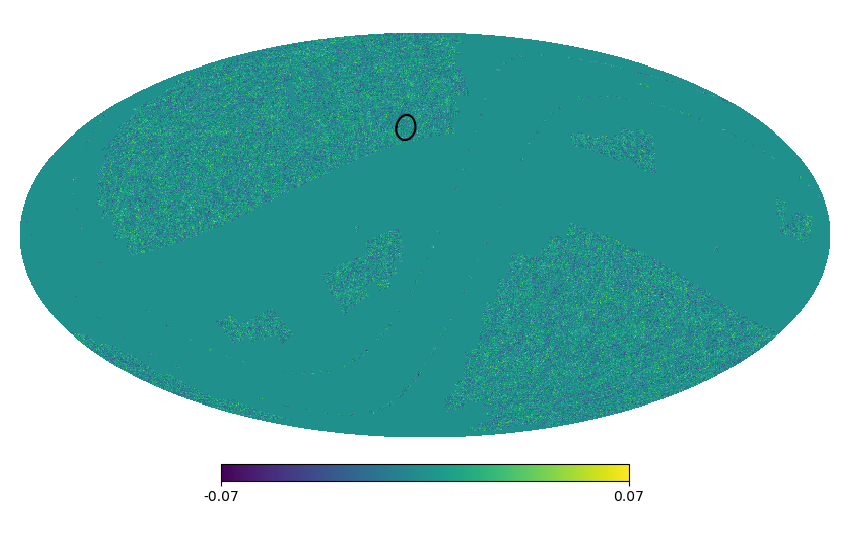
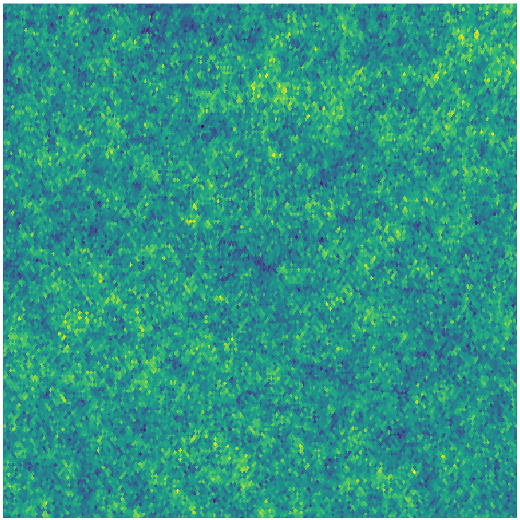
Figure 1: A map of the convergence sampled from a log-normal distribution with power spectrum Eq. (4) and parameters as described in Sect. 4.4. The colors encode the values of the weak-lensing convergence as indicated by the color bar. Left panel: Full sky map in Mollweide projection, ecliptic coordinates, showing the Euclid footprint, see Scaramella et al. [62] for more details. The large bands are the Ecliptic and Galactic plane, which are masked due to dust extinction and zodiacal light. Right plot: Zoom-in of a $10\times 10$ deg² area, marked by the circle in the left image.

The lensing power spectrum of Eq. (4) is the most fundamental observable for cosmological inference as it depends on cosmological parameters in several ways. It is a linear projection of the 3D matter power spectrum $P_{\delta}$, which encodes the matter distribution and its evolution over redshift. The projection kernel is a function of the comoving distance $\chi$, which depends on the matter content and the geometry of the Universe. In addition, it is directly affected by two cosmological parameters: the matter density $\Omega_{\textrm{m}}$ and the Hubble constant $H_{0}$.

The $C_{\ell}$ describes the power in the shear field $\gamma$ as a function of projected Fourier distance on the sky $\ell$. We write in the flat-sky approximation

$$\left\langle\tilde{\gamma}(\bm{\ell})\tilde{\gamma}^{\ast}(\bm{\ell}^{\prime})\right\rangle=\delta_{\textrm{D}}^{(2)}(\bm{\ell}-\bm{\ell}^{\prime})\,C_{\ell},$$ (6)

where $\tilde{\gamma}$ denotes the Fourier transform of $\gamma$, and the superscript ‘^∗’ denotes the complex conjugation. Due to statistical homogeneity, different Fourier modes of the field $\gamma$ are uncorrelated, which is expressed by the 2D Dirac delta distribution $\delta_{\textrm{D}}^{(2)}$. On large scales, $\ell\lesssim 100$, the shear field is very close to Gaussian, and different Fourier modes of the power spectrum are uncorrelated. The $C_{\ell}$ has a maximum at $\ell$ of a few $10$, which corresponds to the size of the horizon at the time of matter-density equality. This is defined as the time in the early Universe when the matter density equals the radiation density, and matter subsequently became dominant, at a redshift of $z_{\rm eq}\approx 31,000\,\Omega_{\mathrm{m}}h^{2}$, in the early Universe. The non-linear regime starts at $\ell\gtrsim 1,000$, marked by an increase of power, and the convergence field becomes non-Gaussian resulting in the power spectrum becoming correlated across different $\ell$-modes. An example of the lensing power spectrum will be presented in Sect. 4.3.1.

2.1.3 The lensing power-spectrum covariance

For the observed lensing power spectrum, $C_{\ell,{\rm obs}}$, we need to account for shot noise, which is due to intrinsic galaxy ellipticities having a non-vanishing dispersion $\sigma_{\varepsilon}$ of typically $0.3$ - $0.4$. We write

$$C_{\ell,{\rm obs}}=C_{\ell}+\frac{\sigma_{\varepsilon}^{2}}{\bar{n}},$$ (7)

In the linear regime for the density contrast, the lensing power spectrum can be approximated by a normal distribution with uncorrelated Fourier modes. The variance in this approximation is

$$\mathbb{E}\left(C_{\ell,\text{obs}}^{2}\right)-\mathbb{E}\left(C_{\ell,\text{obs}}\right)^{2}=\frac{1}{f_{\textrm{sky}}(2\ell+1)}C_{\ell,\text{obs}}^{2},$$ (8)

where $f_{\textrm{sky}}$ is the fraction of the observed sky area [38]. This diagonal covariance matrix will be referred to as the Gaussian covariance.

This Gaussian covariance is appropriate in the regime where the Fourier modes of the lensing field are independent. This is no longer true on small scales, where the non-linear evolution of the density field leads to mode coupling. Further, there is a coupling of non-linear, small scales to long-wavelength modes that can be larger than the observed area. This is due to the finite observed volume, which is not representative of the ensemble, large-scale density fluctuations. These fluctuations induce additional power on small scales, which create the coupling between small and large scales. These mode couplings mean that different modes of the field $\gamma$ are no longer independent, and the distribution of $\gamma$ becomes non-Gaussian. This implies that the covariance of the convergence power spectrum is no longer diagonal. Note that the Fourier modes of $\gamma$ itself are still uncorrelated, since Eq. (6) is based only on the homogeneity of $\gamma$. The small-to-long wavelength mode couplings lead to an additional lensing covariance, which is the dominant non-Gaussian contribution [4]. This term is called super-survey covariance (SSC). Barreira et al. [4] showed that the total weak-lensing power-spectrum covariance is well represented by the Gaussian covariance plus the SSC term, which we refer to as the Gaussian plus SSC covariance.

Eq. (4) is the power spectrum of not only the shear, but of a scalar field called the convergence. This field can be obtained from the shear field, and is more directly related to the density contrast. Fig. 1 shows a realisation of a convergence field, drawn from a log-normal distribution with powe r spectrum Eq. (4). The cosmological parameters and redshift distribution that are used are described in Sect. 4.4. To the full-sky convergence map the footprint mask of the Euclid survey is applied, resulting in a remaining observed area of $f_{\mathrm{sky}}=0.3636$ corresponding to $15,000$ deg². Euclid [45] is a European space experiment, to be launched in early 2023. Euclid will observe $1.5$ billion galaxies in optical and infrared wavelengths. Weak gravitational lensing is one of the two main cosmological observables for Euclid. The Euclid mask cuts out unobserved regions, with the main areas being the Galactic and the Ecliptic plane. These regions on the sky are heavily influenced by dust in the Milky Way disk, and zodiacal light (reflection of sun light by dust particles), respectively. These effects adversely impact the number of observable background galaxies, their flux and their measured shapes.

2.1.4 The lensing likelihood function

We suppose that the observed power spectrum $C_{\ell}$ is measured at $p$ discrete Fourier scales $\ell_{i},i=1\ldots p$. The data vector $\bm{y}=\{C_{\ell_{i}}\}$ is assumed to follow a $p$-dimensional multivariate normal distribution, $\bm{y}\sim{\cal N}_{p}(\bm{m}(\bm{\theta}),\bm{\mathrm{C}})$, with mean $\bm{m}(\bm{\theta})\in\mathbb{R}^{p}$ and $p\times p$ covariance matrix $\bm{\mathrm{C}}$. The mean depends on the parameter vector $\bm{\theta}\in\mathbb{R}^{n_{\theta}}$. The likelihood function $L$ is the usual multivariate normal likelihood given in log form by

$$-\ln L(\bm{y}|\bm{\theta}) =\,{\rm const}+\frac{1}{2}\ln{\rm tr\,}\,\bm{\mathrm{C}}+\frac{1}{2}\chi^{2}(\bm{y}|\bm{\theta});$$

$$\chi^{2}(\bm{y}|\bm{\theta}) =\left[\bm{y}-\bm{m}(\bm{\theta})\right]^{\rm t}\bm{\mathrm{\Psi}}\left[\bm{y}-\bm{m}(\bm{\theta})\right],$$ (9)

which depends on the precision matrix, $\bm{\mathrm{\Psi}}=\bm{\mathrm{C}}^{-1}$. The covariance and precision matrices are considered independent of $\bm{\theta}$.

2.2 Estimators of the covariance and precision matrices

A summary of estimators for the covariance matrix ($\hat{\bm{\mathrm{C}}}$), and a biased ($\hat{\bm{\mathrm{\Psi}}}_{\ast}$) and unbiased ($\hat{\bm{\mathrm{\Psi}}}$) estimator of the precision matrix are displayed in Table 1. Along with the estimators, their first and second moments are also included. Note that throughout we use the notation $\bm{z}^{\mathrm{t}}$ to indicate the transpose of $\bm{z}$, and given some matrix $\bm{\mathrm{Z}}$, $Z_{ij}$ represents the element in the $i$th row and $j$th column of $\bm{\mathrm{Z}}$. In Table 1, the estimators consider simulated realizations of the data vector, $\bm{y}_{j}\in\mathbb{R}^{p}$, with $j=1,\ldots,n_{\rm s}$. The sample mean vector is $\bm{\bar{y}}\in\mathbb{R}^{p}$, where $\bm{\bar{y}}=n_{\rm s}^{-1}\sum_{j=1}^{n_{\rm s}}\bm{y}_{j}$.

For $\bm{y}\sim{\cal N}(\bm{m}(\bm{\theta}),\bm{\mathrm{C}})$, the covariance estimator is $p$-Wishart-distributed, $\nu\hat{\bm{\mathrm{C}}}\sim{\cal W}_{p}(\bm{\mathrm{C}},\nu)$, with degrees of freedom $\nu=n_{\rm s}-1$. The Wishart distribution is well-defined for $\nu>p-1$, for which $\hat{\bm{\mathrm{C}}}$ is invertible. For $\nu\leq p-1$, $\hat{\bm{\mathrm{C}}}$ is singular, and $\hat{\bm{\mathrm{C}}}$ follows a singular or anti-Wishart distribution [51].

A biased estimator of the precision matrix is $\hat{\bm{\mathrm{\Psi}}}_{\ast}$ [69], as displayed in Table 1. This estimator follows an inverse-Wishart distribution, $\nu\hat{\bm{\mathrm{\Psi}}}_{\ast}\sim{\cal W}_{p}^{-1}\left(\bm{\mathrm{\Psi}},\nu\right)$, with degrees of freedom $\nu$. A debiased estimator can be found as $\hat{\bm{\mathrm{\Psi}}}=\left(\nu-p-1\right)\nu^{-1}\hat{\bm{\mathrm{\Psi}}}_{\ast}$. This result has been routinely used to debias the estimated covariance from simulations in weak gravitational lensing [e.g., 26, 36, 44], and cosmology in general [e.g., 24, 57, 25].

Symbol	Description	Form
$\hat{\bm{\mathrm{C}}}$	Covariance	$\hat{\bm{\mathrm{C}}}=\frac{1}{n_{\rm s}-1}\sum_{j=1}^{n_{\rm s}}\left({\bm{y}^{j}}-\bm{\bar{y}}\right)\left({\bm{y}^{j}}-\bm{\bar{y}}\right)^{\rm t}$
	matrix	$\mathbb{E}\hat{\bm{\mathrm{C}}}=\nu\,\bm{\mathrm{S}}=\bm{\mathrm{C}}$
		$\mathbb{E}(\hat{C}_{ij}-C_{ij})^{2}=\nu^{-1}\left(C_{ij}^{2}+C_{ii}C_{jj}\right)$, [61]
$\hat{\bm{\mathrm{\Psi}}}_{\ast}$	Precision	$\hat{\bm{\mathrm{\Psi}}}_{\ast}=\hat{\bm{\mathrm{C}}}^{-1}$
	matrix	$\mathbb{E}(\hat{\bm{\mathrm{\Psi}}}_{\ast})=(\nu-p-1)^{-1}\nu\,\bm{\mathrm{C}}^{-1}$
		for $\nu>p-1$, [61]
		$\mathbb{E}(\hat{\Psi}_{\ast ij}-\Psi_{\ast ij})^{2}=\frac{\nu^{2}\left[\left(\nu-p+1\right)\Psi_{ij}^{2}+(\nu-p-1)\Psi_{ii}\Psi_{jj}\right]}{(\nu-p)(\nu-p-1)^{2}(\nu-p-3)}$,
		for $\nu>p+3$, [14]
$\hat{\bm{\mathrm{\Psi}}}$	Precision	$\hat{\bm{\mathrm{\Psi}}}=\alpha\hat{\bm{\mathrm{\Psi}}}_{\ast}$
	matrix	$\alpha=\frac{\nu-p-1}{\nu}=\frac{n_{\textrm{s}}-p-2}{n_{\textrm{s}}-1}$
		$\mathbb{E}(\hat{\bm{\mathrm{\Psi}}})=\bm{\mathrm{C}}^{-1}$
		$\mathbb{E}(\hat{\Psi}_{ij}-\Psi_{ij})^{2}=\alpha^{2}\mathbb{E}(\hat{\Psi}_{\ast ij}-\Psi_{\ast ij})^{2}$

Table 1: Estimators and two moments for covariance and precision matrices.

To show how the analytical expressions for the variances of the estimators compare to (i) the estimated variances computed based on random draws from the sampling distributions of the estimators and (ii) the estimated variances computed from random draws of the data vector from a multivariate normal, we carried out a comparison by doing the following. Consider a $10\times 10$ identity covariance matrix $\bm{\mathrm{C}}=\bm{\mathrm{I}}_{10}$. We plot the variance of the $(1,1)$-element of $\hat{\bm{\mathrm{C}}}$ (green), $\hat{\bm{\mathrm{\Psi}}}_{\ast}$ (blue), and $\hat{\bm{\mathrm{\Psi}}}$ (red) in Fig. 2. The analytical expressions, shown as lines, are well-reproduced when sampling from ${\cal W}_{10}(\bm{\mathrm{C}},n_{\rm s}-1)$ and ${\cal W}_{10}^{-1}(\bm{\mathrm{C}}^{-1},n_{\rm s}-1)$ (filled symbols). We also sample a vector $\bm{y}$ from a multivariate normal distribution, calculate $\hat{\bm{\mathrm{C}}}$, $\hat{\bm{\mathrm{\Psi}}}_{\ast}$, and $\hat{\bm{\mathrm{\Psi}}}$ using the estimators from Table 1, and the variance of the estimators from the $\nu+1$ simulations (open symbols). The key point is that we can estimate mean and variance of the covariance estimator $\hat{\bm{\mathrm{C}}}$ for $\nu\leq p-1$ by simulating realizations from the appropriate multivariate normal distribution, even in cases where the inverse covariance is no longer defined (green open circles). We make extensive use of this feature in the proposed methodology.

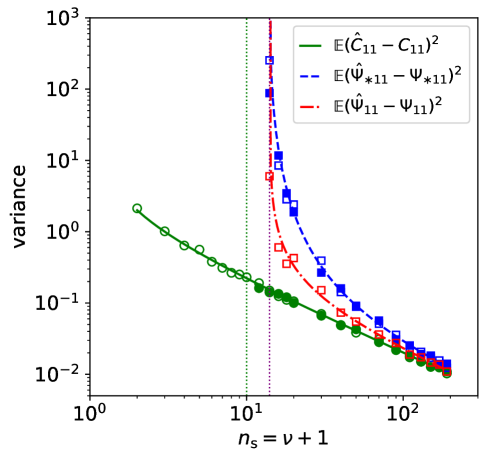
Figure 2: Variance of the Wishart (${\cal W}_{10}$, green solid line/circles) and inverse Wishart (${\cal W}_{10}^{-1}$, dashed blue line/squares) distributions, as function of $\nu+1$. The dash-dotted line and squares show the debiased variance of ${\cal W}_{10}^{-1}$. Values are $(1,1)$ matrix elements, lines analytical expressions, filled symbols samples from ${\cal W}_{10}$ and ${\cal W}_{10}^{-1}$. Open symbols use samples from ${\cal N}$. The vertical lines indicate the limit of ${\cal W}_{10}$ (${\cal W}_{10}^{-1}$), at $\nu=p-1$ ($\nu=p+3$).

3 Approximate Bayesian Computation (ABC)

Some of the problems that plague traditional likelihood-based inference methods can be circumvented with Approximate Bayesian Computation [ABC; 72, 59, 8, 6]. Rather than specifying a likelihood function, ABC works by drawing samples from a simulation model, $\bm{y}_{\text{sim}}\sim M(\bm{\theta})$. The basic ABC algorithm [72, 59] samples values of $\bm{\theta}^{*}$ from some user-specified prior(s), $\pi(\bm{\theta})$, generating a simulated dataset $\bm{y}_{\text{sim}}\sim M(\bm{\theta}^{*})$, and then comparing $\bm{y}_{\text{sim}}$ to the observed dataset, $\bm{y}_{\text{obs}}$. If $\bm{y}_{\text{sim}}$ and $\bm{y}_{\text{obs}}$ are “close enough” (discussed more specifically below), then $\bm{\theta}^{*}$ is retained and contributes to the particle approximation of the posterior distribution of $\bm{\theta}$.

For the simulation model, the likelihood function need not to be known explicitly. For example, the simulation model could, in theory, be derived from $N$-body simulations if they were computationally feasible for use in an ABC algorithm (which they are not). Since $N$-body simulations are too computationally intensive, fast approximate simulations could be used instead. The simulations generate realizations of observables through a complex forward process that mimics the gravitational interactions in an expanding Universe.

ABC can also be carried out by replacing a complex likelihood-free simulation model with sampling from an explicitly chosen distribution (from which a likelihood function $L$ would be based). The advantage in this case over MCMC is that $L$ does not need to be evaluated. In particular, if the chosen distribution is a multivariate normal, the precision matrix is not required which is important in our setting.

We compare ABC-based parameter estimates and their uncertainties to the corresponding Fisher matrix-based and MCMC-based quantities. We assume that we have simulated $n_{\rm s}$ independent multivariate normal random vectors from which we compute an estimate of the covariance matrix using $\hat{\bm{\mathrm{C}}}$ from Table 1. The Fisher matrix and MCMC then require the evaluation of a likelihood function together with an estimate of the precision matrix. For ABC we need only to generate data vectors from a simulation model, which do not depend on $\hat{\bm{\mathrm{\Psi}}}$, but only on $\hat{\bm{\mathrm{C}}}$. We demonstrate that inference using ABC is possible when $\nu\leq p+1$, even for $p/\nu>100$, and the results do not appear to depend on $\nu$.

3.1 ABC algorithm

The basic ABC algorithm discussed above can be computationally inefficient so a number of extensions of this algorithm have been proposed (e.g., Sisson et al. 70, Beaumont et al. 7, Moral et al. 54, Bonassi and West 9). In this work, we use the CosmoABC implementation of the ABC-Population Monte Carlo (ABC-PMC) algorithm [7] described in [30].

ABC-PMC starts with the basic ABC algorithm in iteration $t=1$ where samples of a $n_{\theta}$-dimensional parameter vector $\bm{\theta}$ are proposed from the prior distribution, $\pi(\bm{\theta})$. Simulated data, $\bm{y}_{\text{sim}}$, are generated from the simulation model using a proposed $\bm{\theta}^{*}$, and are then compared to the observations, $\bm{y}_{\text{obs}}$, via a distance function $D(\cdot,\cdot)$. Often the distance function uses summaries $\bm{s}(\cdot)$ of the simulated and observations rather than the data themselves. The distance functions developed for our setting are discussed in Sect. 3.3. If $D[\bm{s}(\bm{y}_{\text{sim}}),\bm{s}(\bm{y}_{\text{obs}})]\leq\epsilon_{t}$, where $\epsilon_{t}$ is a tolerance value for iteration $t$, then the proposed $\bm{\theta}^{*}$ is retained; otherwise it is discarded. This is repeated until $M$ values are accepted, $\{\bm{\theta}^{(j)}\}_{j=1}^{M}$.

In subsequent iterations $t=2,\ldots,T$, rather than drawing directly from $\pi(\bm{\theta})$, the previous iteration’s ABC posterior is used where the selected values are moved according to a user-specified kernel, $K(\bm{\theta},\cdot)$ (in our case, a Gaussian kernel). Importance weights are defined to account for this change in proposal distribution after the initial use of the prior in step $t=1$, and the resulting ABC posterior distribution is based on the particle system $\{\bm{\theta}_{t}^{(j)},W_{t}^{(j)}\}_{j=1}^{M}$ where $W_{t}^{(j)}$ are the importance weights such that $\sum_{j=1}^{M}W_{t}^{(j)}=1$. We update the distance threshold $\epsilon_{t+1}$ of iteration $t+1$ as the $q$ percentile of the distances in iteration $t$, with $q=0.75$.

For the stopping criterion, at each iteration the number of accepted particles divided by the number of proposed particles, $\delta_{t}$, is computed. If $\delta_{t}<\delta_{0}$, where $\delta_{0}$ is a user-specified threshold, the sampling is stopped, which occurs when the number of draws exceeds the number of particles by $1/\delta_{0}$. We refer the reader to Ishida et al. [30] for a detailed description of the algorithm.

3.2 Simulation set-up

3.2.1 Data generation

For all our experiments, we simulate observation $\bm{d}_{\text{obs}}=(\bm{x}_{\text{obs}},\bm{y}_{\text{obs}})$, with $\bm{x}_{\text{obs}}=({x_{\text{obs}}}_{,1},\ldots,$ ${x_{\text{obs}}}_{,p})$ and $\bm{y}_{\text{obs}}=({y_{\text{obs}}}_{,1},\ldots,{y_{\text{obs}}}_{,p})$, as follows. We fix the abscissa vector $\bm{x}_{\text{obs}}$, and the $p\times p$ covariance matrix $\bm{\mathrm{C}}$. Then we generate $n_{\textrm{r}}$ independent draws of the observed ordinate vectors $\bm{y}^{r}_{\text{obs}}$, $r=1\ldots n_{\textrm{r}}$ as multivariate normal random variable, $\bm{y}^{r}_{\text{obs}}\sim{\cal N}(\bm{m}(\bm{\theta}_{0}),\bm{\mathrm{C}})$. The mean is the model prediction for a given fixed model parameter vector $\bm{\theta}_{0}$. Next, for each $r$ and given a simulation sample size $n_{\textrm{s}}=\nu-1$ we compute the sample covariance $\hat{\bm{\mathrm{C}}}$. If $p\leq\nu$, we can sample directly from a Wishart distribution, $\hat{\bm{\mathrm{C}}}\sim{\cal W}_{p}(\bm{\mathrm{C}},\nu)$. For $p>\nu$, we instead generate $n_{\rm s}$ multivariate normal random variables $\bm{y}^{j}\sim{\cal N}(\bm{y}^{r},\bm{\mathrm{C}})$, and compute $\hat{\bm{\mathrm{C}}}$ according to Table 1.

3.2.2 ABC sampling details

To create the initial ABC set of particles we draw $2M$ values from the prior, and retain the $M$ particles that result in the lowest distance. Each subsequent ABC-PMC iteration uses $M$ particles. For each simulated observation corresponding to a proposed parameter vector $\bm{\theta}^{*}$, we create a model prediction $\bm{y}_{\text{sim}}(\bm{\theta}^{*})\sim{\cal N}(\bm{m}(\bm{\theta}^{*}),\hat{\bm{\mathrm{C}}})$, where $\hat{\bm{\mathrm{C}}}$ is the sample covariance matrix generated earlier (which is singular for $p<\nu$).

3.3 Summary statistics and distances

The cases discussed in this work simulate one-dimensional functions $f:\mathbb{R}\rightarrow\mathbb{R}$, mimicking the weak-lensing power spectrum $C_{\ell}$ of Eq. (4). The data vectors are composed of joint abscissa and ordinate vectors, $\bm{d}_{\text{Z}}=(\bm{x}_{\text{Z}},\bm{y}_{\text{Z}})$, Z $\in$ {obs, sim}, where the two identifiers stand for observation and simulation, respectively.

In the following we introduce the distance functions used in this work, that do not depend on the estimated precision matrix. We propose simple distance functions that ignore any correlation between data points, and also a new distance function that accounts for correlation without depending on $\hat{\Psi}$.

3.3.1 Parameter-based distance function

For a function $f$ which can be described by a parameter vector $\bm{\theta}\in\mathbb{R}^{n_{\theta}}$, a distance function can be constructed based on parameter estimates as follows. For a given set of simulated data vectors $\bm{d}_{\text{sim}}=(\bm{x}_{\text{sim}},\bm{y}_{\text{sim}})$, the function $f$ is fitted with $\hat{\bm{\theta}}_{\text{sim}}$, which is obtained from an ordinary least squares regression. An analogous fit is performed on the observed data to yield the best-fit parameter $\hat{\bm{\theta}}_{\text{obs}}$. For this case, the summary statistic depends on the best-fit parameters,

$$\bm{s}_{\rm param}(\bm{d})=\hat{\bm{\theta}},$$ (10)

corresponding to a compression of the data into $n_{\theta}$ values. Then, the parameter distance $D_{\rm param}$ is

$$D_{\rm param} [\bm{s}_{\rm param}(\bm{d}_{\text{obs}}),\bm{s}_{\rm param}(\bm{d}_{\text{sim}})]=\sqrt{\sum_{i=1}^{n_{\theta}}\left[{\theta_{\text{obs}}^{\ast}}_{,i}-{\theta_{\text{sim}}^{\ast}}_{,i}\right]^{2}}.$$ (11)

3.3.2 Covariance-based distance function

A more general summary statistic $\bm{s}$, which uses the full data vector, is

$$\bm{s}(\bm{d})=\bm{y}.$$ (12)

A general distance function is the Mahalanobis distance $D_{\bm{\mathrm{\Psi}}}$, given as

$$D_{\bm{\mathrm{\Psi}}}[\bm{s}(\bm{d}_{\text{obs}}),\bm{s}(\bm{d}_{\text{sim}})]=\sqrt{\Delta\bm{y}^{\rm t}{\bm{\mathrm{\Psi}}}\Delta\bm{y}},$$ (13)

where

$$\Delta\bm{y}=\bm{y}_{\text{obs}}-\bm{y}_{\text{sim}}$$ (14)

This distance can however not be used if the true precision matrix is not known and the estimated covariance matrix is singular. We therefore have to find an alternative distance. A distance derived from Eq. (13) can be obtained by replacing the precision matrix by a diagonal matrix with the reciprocal elements of the estimated covariance matrix $\hat{C}$ on the diagonal. This results in the inverse-variance distance function

$$D_{\hat{C}}[\bm{s}(\bm{d}_{\text{obs}}),\bm{s}(\bm{d}_{\text{sim}})]=\sqrt{\sum_{i}\left(\frac{\Delta y_{i}}{\hat{C}_{ii}}\right)^{2}},$$ (15)

The diagonal elements $\hat{C}_{ii}$ are non-zero even in the case where $\hat{\bm{\mathrm{C}}}$ is singular.

3.3.3 Autocorrelation-based distance function

Next, we introduce a new distance that accounts for the correlation of data points but does not require the inversion of the covariance matrix. Note that with this distance the covariance matrix is only used to generate the simulated data. This distance is based on the autocorrelation function (acf) of the data $\bm{y}_{\text{obs}}$, which is a function of lag $t$. We define the unnormalised acf as

$$\xi_{\bm{y}}^{\textrm{u}}(t)=\frac{1}{(p-t)}\sum_{i=1}^{p-t}\left(y_{i}-\bar{y}^{(1,p-t)}\right)\,\left(y_{i+t}-\bar{y}^{(t+1,p)}\right);\quad\quad t=0\ldots p-1,$$ (16)

where we subtract from each shifted data vector the corresponding mean,

$$\bar{y}^{(m,n)}=\frac{1}{(m-n)}\sum_{i=m}^{n}y_{i}.$$ (17)

The function $\xi_{\bm{y}}^{\textrm{u}}(t)$ is normalised such that its value is unity at $t=0$, which gives the acf as the following

$$\xi_{t}(\bm{y})=\frac{\xi_{t}^{\textrm{u}}(\bm{y})}{\xi_{0}^{\textrm{u}}(\bm{y})}.$$ (18)

The acf quantifies the mean autocorrelation of the data between two entries with indices separated by $t$, in the case of equidistant abscissa; this difference is $\Delta x=x_{i+t}-x_{i}$ for all $i$. The autocorrelation is used in the distance function to penalize data points that are strongly correlated with others by increasing the overall distance. The acf distance is defined as

$$D_{\rm acf} [\bm{s}(\bm{d}_{\text{obs}}),\bm{s}(\bm{d}_{\text{sim}})]=\left|\sum_{i,j=1}^{{n_{\textrm{d}}}}\Delta y_{i}\,\xi_{|i-j|}\,\Delta y_{j}\right|.$$ (19)

This distance accounts for the correlation between data points without depending on the precision matrix. For a given difference between data points indices $t=|i-j|$, the acf $\xi_{|i-j|}$ contributes to the distance as a weight, and represents the average correlation corresponding to that $t$. Summands in Eq. (19) with $i=j$ contribute maximally to the distance, with unit weight $\xi_{0}=1$. Off-diagonal terms with $i\neq j$ that are not correlated do not contribute significantly to the distance; the intuition is that the distance should not be influenced by the difference between uncorrelated data points. On the other hand, two correlated data points with $0<\xi_{|i-j|}\leq 1$ contribute to the overall distance, by penalising models that predict $y_{{}_{\text{sim}},i}$ to be very different from $y_{{}_{\text{obs}},j}$.

4 Simulation Study

In this section we present three simulation experiments to evaluate the performance of the proposed ABC method. We investigate the uncertainty in the covariance matrix estimation, and its propagation to the parameter estimates, their standard errors, and the uncertainty in the parameter estimates’ errors (i.e., the uncertainty in the uncertainty). All three experiments simulate one-dimensional functions, where the abscissa values are drawn from a multivariate normal distribution with a given covariance matrix. A flat prior is used in each of the $n_{\theta}=2$ dimensions of $\bm{\theta}$. Next, we describe different methods for comparison with the proposed ABC approach.

4.1 Comparison methods

The performance of the proposed ABC method is compared to a Fisher information matrix approach where the Fisher matrix is computed for a multivariate normal distribution. The Fisher matrix is computed at the (true) input values for the parameters. For the first example, a Metropolis-Hastings Monte-Carlo Markov Chain (MCMC) sampling approach is also considered, and the parameter estimates are based on the posterior mean.

For the multivariate normal distribution of Eq. (9), if the data covariance $\bm{\mathrm{C}}$ does not depend on $\bm{\theta}$, the Fisher matrix $\bm{\mathrm{F}}$ is given as [10]

$$\bm{\mathrm{F}} =\bm{\mathrm{M}}^{\textrm{t}}\bm{\mathrm{\Psi}}\bm{\mathrm{M}}$$ (20)

with $M_{ij}=\partial m_{i}/\partial\theta_{j}$, see Tegmark et al. [75] for a seminal discussion in a cosmology context. When the true precision matrix $\bm{\mathrm{\Psi}}$ is replaced by $\hat{\bm{\mathrm{\Psi}}}_{\ast}$ and $\hat{\bm{\mathrm{\Psi}}}$ (see Table 1), the corresponding estimated Fisher matrices are denoted as $\hat{\bm{\mathrm{F}}}_{\ast}$ and $\hat{\bm{\mathrm{F}}}$, respectively. The parameter covariance (estimate) is obtained by inverting the Fisher matrix (estimate), see App. A for more details.

The likelihood is no longer multivariate normal if the true precision matrix $\bm{\mathrm{\Psi}}$ is replaced by an estimate. Instead, a Hotelling $T^{2}$ likelihood function is appropriate [see 29, 52]. This distribution was also derived in Sellentin and Heavens [65], where they marginalise the multivariate normal likelihood over the Wishart distribution of the estimated inverse covariance matrix. The resulting log-likelihood is

$$-\ln L_{T^{2}}(\bm{y}|\bm{\theta})=\,{\rm const}+\frac{\nu+1}{2}\ln\left[1+\frac{\chi^{2}_{\ast}(\bm{y}|\bm{\theta})}{\nu}\right],$$ (21)

where $\chi^{2}_{\ast}$ is similar to the term given in Eq. (9), but with the estimated (biased) inverse covariance $\hat{\bm{\mathrm{\Psi}}}_{\ast}$ instead of $\bm{\mathrm{\Psi}}$.

For our first simulation study (Sect. 4.2), we explore the multivariate normal of Eq. (9) and Hotelling $T^{2}$ likelihood of Eq. (21) with a Metropolis-Hastings Monte-Carlo Markov Chain sampler, implemented in stan [11]. For each number of simulations $n_{\rm s}$ used for the covariance estimation, we produce $n_{\rm r}=50$ independent MCMC runs. We compute the convergence of the samples by running three chains with $2,000$ points for each run, after discarding the first $1,000$ burn-in phase chain points.

4.2 Experiment: affine function with diagonal covariance matrix

With this experiment we explore the capability of the proposed ABC algorithm to infer parameters compared to likelihood-based approaches using a model with a diagonal covariance matrix.

4.2.1 Data-generating model

We consider an affine function model $\bm{m}(\bm{\theta})=a\bm{x}+b\bm{1}$, where the slope $a$ and intercept $b$ are the model parameters $\bm{\theta}=(a,b)$. The input model is set to $\theta_{0}=(1,0)$. As described in Sect. 3.2.1, we fix the abscissa vector $\bm{x}$ and covariance matrix $\bm{\mathrm{C}}$. The former are generated once by drawing $p=750$ uniform variables $x_{i},i=1\ldots p$, $x_{i}\sim{\cal U}(-\Delta/2;\Delta/2)$ with $\Delta=200$. Note that this precludes the use of the acf distance, which requires an equidistantly spaced $\bm{x}$. The input covariance matrix is the diagonal, matrix

$$\bm{\mathrm{C}}=\sigma^{2}\bm{\mathrm{I}}_{p}.$$ (22)

Here, $\bm{\mathrm{I}}_{p}$ is the $p\times p$ identity matrix, and we fix the value of the variance as $\sigma^{2}=5$.

4.2.2 Distance function

We use the parameter summary statistic of Eq. (10) and the corresponding distance function, $D_{\text{param}}$ from Eq. (11), with parameter $\bm{\theta}=(a,b)$. We carry out one modification to the distance function since we found that using the absolute value of $b$ improves the convergence and the resulting errors on $b$. The modified parameter distance is then

$$D^{\prime}_{\rm param} [\bm{s}_{\rm param}(\bm{d}_{\text{obs}}),\bm{s}_{\rm param}(\bm{d}_{\text{sim}})]=\sqrt{(a_{\text{obs}}^{\ast}-a_{\text{sim}}^{\ast})^{2}+(|b_{\text{obs}}^{\ast}|-|b_{\text{sim}}^{\ast}|)^{2}}.$$ (23)

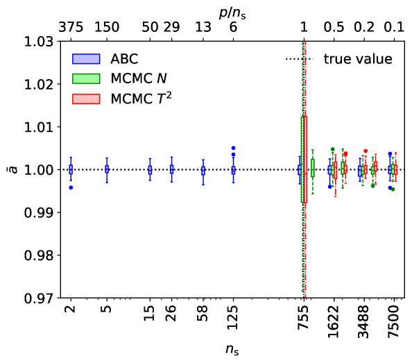
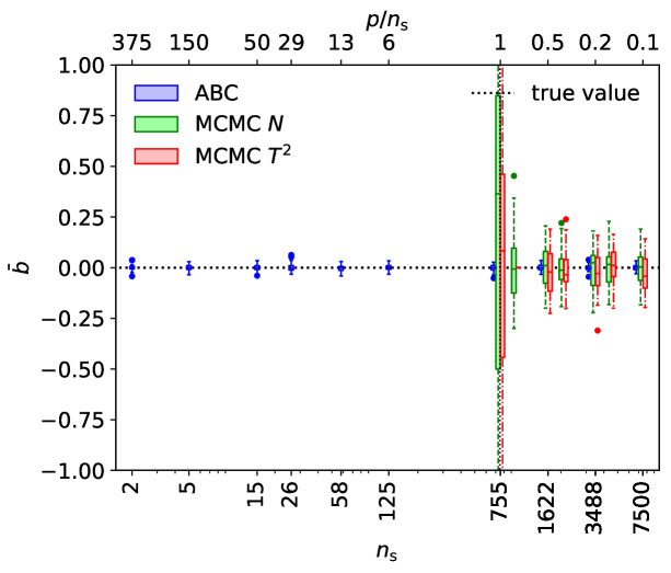
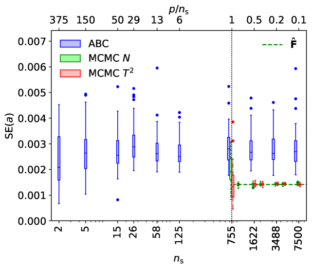
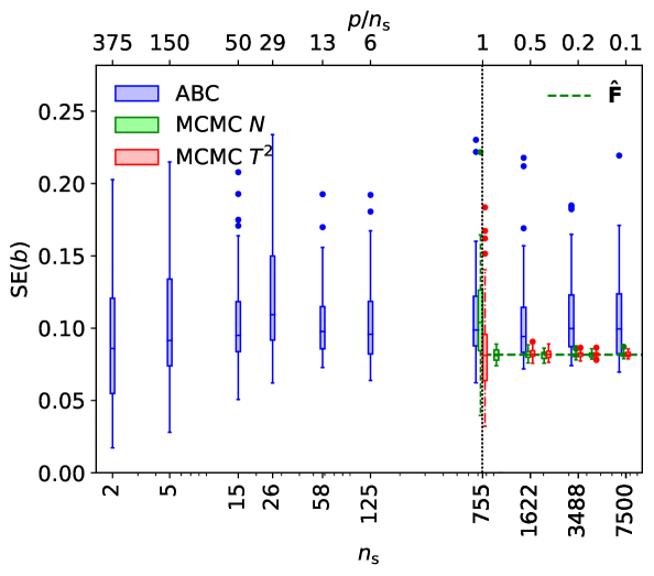
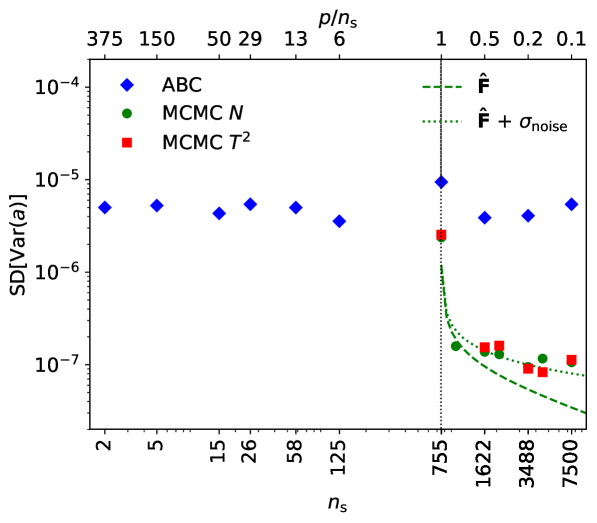
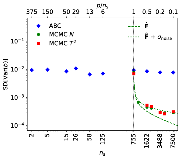
Figure 3: Mean (top row), SE (middle) and SD of the variance (bottom) of the parameter estimates of $a$ (left column) and $b$ (right column). Results are shown for ABC (solid blue boxes, diamonds), and MCMC sampling of the normal ($T^{2}$) likelihood with dashed green lines and circles (dash-dotted red lines and squares). Each point corresponds to a number of simulations $n_{\textrm{s}}$ used for the covariance estimate, and its inverse for MCMC sampling. The top panels show the true input values for $a$ and $b$ as dotted lines. The middle panels display Fisher-matrix prediction for the normal likelihood with dashed lines. The bottom plots show as dashed line the prediction for the normal likelihood (A.1) and the dotted line has added Monte-Carlo noise (see §4.2.4).

4.2.3 Experiment details

We use $M=100$ points in each PMC iteration after the first, and a convergence criterion of $\delta=0.025$. This leads to a typical number of $\sim 36$ iterations. The total number of proposed particles, for which the distance needs to be computed, is around $30,000$, corresponding to a overall acceptance rate of $0.12$. For comparison, we explore the multivariate normal likelihood from Eq. (9) and Hotelling $T^{2}$ likelihood from Eq. (21) with a Metropolis-Hastings MCMC sampler as discussed in Sect. 4.1.

4.2.4 Results

Fig. 3 shows the average estimate $\bar{\bm{\hat{}}{\theta}}$, the standard error SE($\bm{\hat{}}\theta)$, and the standard deviation of the variance SD$[$Var$(\bm{\hat{}}\theta)]$ of the parameter $\bm{\theta}=(a,b)$, for ABC and the likelihood-based comparison methods. From the $n_{\textrm{r}}=50$ runs we obtain the distribution of the mean and standard errors, shown as box plot. We estimate SD$[$Var$(\bm{\hat{}}\theta)]$ as the standard deviation over the $50$ estimates of Var($\bm{\hat{}}\theta)$. The plot suggests unbiased mean estimates for both $a$ and $b$ for all methods considered, even for a singular covariance when $p\geq n_{\rm s}$ for the proposed ABC method. This is true down to the extreme case of $n_{\rm s}=2$, corresponding to a ratio $p/n_{\rm s}=375$. The SE estimates for ABC are larger compared to the multivariate normal prediction, see Sects. 4.1 and A.2. No significant dependence on the number of simulations $n_{\rm s}$ for the covariance computation is visible.

For the normal and $T^{2}$ likelihood the estimated SD$[$Var$(\hat{\bm{\theta}})]$ is biased high compared to the Fisher-matrix prediction, derived in A.1. There is additional variance intrinsic to Monte-Carlo sampling that does not stem from the inversion of the covariance. We estimate this uncertainty by evaluating the normal likelihood function with the true precision matrix $\bm{\mathrm{\Psi}}=\sigma^{-2}\bm{\mathrm{I}}_{p}$. We find a distribution of the variances of the parameter estimators with finite width, reflecting the sampling noise, which we estimate as SD${}_{\mathrm{noise}}[$Var$(\hat{a})]=4.6\times 10^{-8}$, and SD${}_{\mathrm{noise}}[$Var$(\hat{b})]=1.75\times 10^{-4}$, with around $10\%$ uncertainty on these values. When this is added to the predicted SD[Var] values (dotted lines in Fig. 3), there is good agreement with the Fisher-matrix prediction.

The normal likelihood has a smaller estimated SD$[$Var$(\hat{\bm{\theta}})]$ compared to ABC, and decreases with increasing $n_{\mathrm{s}}$. The SE of the estimators diverge for both the normal and the Hotelling $T^{2}$ likelihood at $n_{\rm s}=p$. The SD$[$Var$(\hat{\bm{\theta}})]$ from ABC are larger than the ones corresponding to sampling under either likelihood, but do not show a significant dependence on $n_{\mathrm{s}}$ remaining more or less constant down to $n_{\mathrm{s}}=2$.

4.3 Experiment: a weak-gravitational-lensing inspired case

The model for the experiment discussed in this section approximates more closely the statistical properties of weak-gravitational lensing data, in particular the cosmic shear power spectrum observable, $C_{\ell}$, where $\ell$ is the 2D Fourier wave number on the sky. In this study, two distance function options are considered to compare their performances, including assessing the usefulness of accounting for correlations in the data points.

4.3.1 Data-generating model

This example is an analytical model that mimics a weak-lensing power spectrum $C_{\ell}$ (Sect. 4.3). With respect to the previous example (Sect. 4.2), additional complexity typically arising for weak lensing is included: First, the model is non-linear in the parameters, and second, data points are correlated. We follow Sect. 3.2.1 to generate the data vectors for this experiment. The following quadratic function is considered

$$q(x)=c+a(x-x_{0})^{2},$$ (24)

which is a rough approximation of $\log_{10}\left(\ell C_{\ell}\right)$, where we identify $x\equiv\log_{10}\ell$. In Fig. 4, we fit the parabola of Eq. (24) to a weak-lensing power spectrum model, obtained with the software nicaea [41].

Two parameters are defined that reproduce the effect of the main cosmological parameters on $C_{\ell}$, as follows. First, a tilt parameter $t$ corresponds to the matter density $\Omega_{\rm m}$. The matter density determines the epoch of matter-radiation equality in the early Universe, which is responsible (among other factors) for the peak in $C_{\ell}$. For a larger $\Omega_{\rm m}$, the matter-dominated phase starts earlier, and suppression of power in the radiation-dominated era on small scales (large $\ell$) is reduced, shifting the peak to the right. The tilt is proportional to the shift parameter $x_{0}$ in Eq. (24). Second, an amplitude parameter $A$ mimics the 3D density power-spectrum normalisation $\sigma_{8}$. To first-order, $C_{\ell}\propto\sigma_{8}^{2}$, and thus $A$ is given by twice the logarithm of the constant term $c$ in Eq. (24).

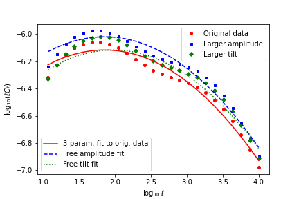
Figure 4: Weak-lensing power spectrum $C_{\ell}$ (points), and best-fit quadratic functions (lines) from Eq. (24). The red circles correspond to parameters $\Omega_{\rm m}=0.306$ and $\sigma_{8}=0.827$. For the blue squares (green diamonds), the values of $\sigma_{8}$ ($\Omega_{\rm m}$) are increased by $10\%$. The dashed and dotted lines are the best-fit curves with free amplitude and tilt, respectively.

Choosing the proportionality constants between $t,A$, and the parabola parameters such that the best-fit values of $t$ and $A$ corresponds to the input model parameters $\Omega_{\rm m}=0.306$ and $\sigma_{8}=0.827$, we find

$$x_{0}=6.05\,t;\quad\quad c=2\log_{10}A-5.95,$$ (25)

where $a=-0.176$ in Eq. (24) is fixed. Fig. 4 shows that changing $\Omega_{\rm m}$ and $\sigma_{8}$ by a small amount can be reproduced by changing $t$ and $A$ by similar amounts, without modifying the other parameters.

Such an approximation would not be acceptable for cosmological modeling, but is sufficient for this experiment because we are mainly interested in a simple and analytical example that roughly reproduces cosmological effects.

The abscissa $\bm{x}$ of the data vector (see Sect. 3.3) consists of $p=10$ values $x_{i}=\ell_{i}$, equally spaced in $\ell$ between $\ell_{\rm min}=25$ and $\ell_{\rm max}=4,000$. The ordinate vector is chosen to mimic the $C_{\ell}$. In this approximation for the weak-lensing power spectrum, this corresponds to

$$m_{i}=10^{q(\log_{10}\ell_{i})}\ell_{i}^{-1}=10^{q(x_{i})-x_{i}}.$$ (26)

As described in Sect. 3.2.1, $n_{\textrm{r}}$ independent observable vectors are generated as multivariate normal, $y_{\text{obs}}^{r}\sim{\cal N}(\bm{m}(\bm{\theta}_{0}),\bm{\mathrm{C}})$. The fixed model parameter vector is $\bm{\theta}_{0}=(t_{0}=0.306,A_{0}=0.827)$.

Two scenarios are used for the uncertainty and correlations between data points in our model. First, we use the diagonal Gaussian covariance matrix with elements according to Eq. (8), where the data points are uncorrelated. Then we consider the Gaussian plus SSC covariance (see Sect. 2.1.3) to model the non-Gaussian and non-linear evolution of the weak-lensing power spectrum on small scales.

For the Gaussian term we mimic the weak-lensing Gaussian covariance given by Eq. (7) and Eq. (8), where we insert $y$ from Eq. (26) for the “signal” $C_{\ell}$. For the SSC term, we use the one derived in Barreira et al. [5], and parameterize the SSC contribution scaled by the weak-lensing power spectrum, see Fig. 3 in Barreira et al. [5]. The correlation matrix of the total covariance (Gaussian + SSC) is plotted in Fig. 6.

To set the numerical values in the covariance matrix, Eqs. (7) and (8), we model a survey with properties similar to what is expected for Euclid [45, 17] with $f_{\textrm{sky}}=0.3636$, corresponding to a observed sky area of $15,000$ deg². The galaxy density in the single redshift bin is chosen as $\bar{n}=30$ arcmin^-2, the intrinsic ellipticity dispersion set to $\sigma_{\varepsilon}=0.31$.

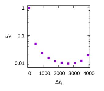
Figure 5: A realization of the normalized auto-correlation function $\xi_{t}$ (18). The x-axis shows the corresponding angular scale difference $\Delta\ell_{t}=\ell_{i+t}-\ell_{i}$, which is independent of $i$.

4.3.2 Distance function

Because the data are correlated in this setting, we consider the acf distance function of Eq. (19). The results are compared with the inverse-variance distance of Eq. (15), which ignores the correlation in the data. The acf of one of the $n_{\textrm{r}}=25$ realizations of the observations $\bm{y}_{\text{sim}}$ is displayed in Fig. 5. After a sharp drop from zero lag, the correlation stays above zero. This represents the correlation between small and large scales (large $\Delta\ell_{t}$), which can be seen in the covariance matrix (Fig. 6). The acf can thus capture some of the correlation information of the data vector, to be used in the distance function.

4.3.3 Experiment details

As in the previous example, each PMC iteration after the first is carried out with $M=100$ accepted particles. To reach convergence, we use a slightly tighter convergence criterion of $\delta=0.015$ resulting in a mean number of iterations to reach convergence of $32$. The total number of draws per run is $40,000$, corresponding to an overall acceptance rate of around $0.08$. The focus of this experiment is the comparison of different ABC distances regarding correlations in the data. Sect. 4.2.4 has established the accuracy of our Fisher-matrix prediction by comparing those with MCMC sampling, which we do not repeat here. Instead, we only compare ABC to the Fisher matrix, see A.3 for the expressions for this example.

$\bm{\mathrm{C}}$	dist.	infer.	$n_{\textrm{s}}$	$\bar{\hat{t}}$	SE$(\hat{t})$	SD$[$Var$(\hat{t})]$	$\bar{\hat{A}}$	SE$(\hat{A})$	SD$[$Var$(\hat{A})]$
G	$\hat{\bm{\mathrm{\Psi}}}$	$\hat{\bm{\mathrm{F}}}$	$\leq p$	-	not computable		-	not computable
			$>p$	-	$0.0007$	$2.9\cdot 10^{-7}$	-	$0.0019$	$2.2\cdot 10^{-6}$
G	diag $\!\hat{\bm{\mathrm{C}}}$	ABC	$\leq p$	$0.3058$	$0.0007$	$2.4\cdot 10^{-7}$	$0.8275$	$0.0019$	$1.8\cdot 10^{-6}$
			$>p$	$0.3059$	$0.0008$	$2.3\cdot 10^{-7}$	$0.8275$	$0.0022$	$2.0\cdot 10^{-6}$
G+SSC	$\hat{\bm{\mathrm{\Psi}}}$	$\hat{\bm{\mathrm{F}}}$	$\leq p$	-	not computable		-	not computable
			$>p$	-	$0.0007$	$3.3\cdot 10^{-7}$	-	$0.0039$	$9.1\cdot 10^{-6}$
G+SSC	diag $\!\hat{\bm{\mathrm{C}}}$	ABC	$\leq p$	$0.3060$	$0.0012$	$5.3\cdot 10^{-7}$	$0.8265$	$0.0043$	$9.8\cdot 10^{-6}$
			$>p$	$0.3061$	$0.0013$	$7.2\cdot 10^{-7}$	$0.8260$	$0.0050$	$8.7\cdot 10^{-6}$
G+SSC	acf	ABC	$\leq p$	$0.3056$	$0.0024$	$2.4\cdot 10^{-6}$	$0.8266$	$0.0049$	$1.3\cdot 10^{-5}$
			$>p$	$0.3055$	$0.0025$	$1.6\cdot 10^{-6}$	$0.8266$	$0.0054$	$1.1\cdot 10^{-5}$

Table 2: Results for the weak-lensing inspired example of Sect. 4.3. Columns: $\bm{\mathrm{C}}$: The covariance matrix used in the model, Gaussian (G), or Gaussian plus super-survey covariance (G+SSC); dist: The covariance component of the distance function; the corresponding equations are Eq. (20) for the Fisher matrix of the normal likelihood; Eq. (15) for the inverse-variance distance; and Eq. (19) for the acf distance, which does not depend on the covariance matrix; infer.: Inference method; $n_{\textrm{s}}$: Simulation size compared to the data vector length $p$. $\hat{t}$, $\hat{A}$: Mean of tilt and amplitude estimates. SE$(\hat{t})$, SE$(\hat{A})$: Standard error of tilt and amplitude estimate. SD$[$Var$(\hat{t})]$, SD$[$Var$(\hat{A})]$: Standard deviation of the variance of tilt and amplitude estimates; The true input values are $t=0.306$ and $A=0.827$. For the Fisher matrix we use Eq. (29) to obtain SD[Var]. Highlighted cells correspond to a singular covariance.

4.3.4 Results

Fig. 7 shows ABC under the non-Gaussian covariance model (G+SSC) with the acf distance Eq. (19). In all cases the ABC parameter estimates are consistent with the true values. The results are summarized in Table 2 for different distance functions and compared using the Fisher-matrix estimates. We average over $n_{\textrm{r}}=25$ runs, and two ranges of the number of simulations: (1) the values $n_{\textrm{s}}=2,5,10$, written as “$\leq p$” in the table; and (2) the values $n_{\textrm{s}}=20,40$, denoted by “$>p$”. For (2) the covariance matrix is non-singular, and thus only this case is available for the Fisher-matrix predictions.

For a Gaussian input model covariance ABC (with the inverse-variance distance (Eq. (15)) shows standard errors (SE) of the parameter estimates close to the Cramér-Rao bound.

With correlated data points via the addition of the SSC term, under the normal likelihood, the SE for the estimated tilt $\hat{t}$ is similar than for the uncorrelated case. However, the SE of the amplitude estimate $\hat{A}$ doubles. With ABC and the inverse-variance distance the SE of $\hat{t}$ $\hat{A}$. Using the acf distance the SE($\hat{t}$) doubles, but the SE$(\hat{A})$ increases only by a small amount.

Table 2 also shows the standard deviation of the variance with the different $n_{\textrm{s}}$ cases. The acf distance results in larger variations compared to the inverse-variance distance. No systematic increase is visible for the case of singular covariance, and the values are relatively independent of $n_{\textrm{s}}$, see Fig. 7. This is not the case for the Fisher-matrix prediction, as already seen in the previous example, and SD[Var] diverges for $n_{\textrm{s}}=p+2$.

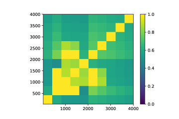
Figure 6: Correlation coefficient of the total covariance matrix (Gaussian + SSC). The axis labels show the values of $\ell$.

To summarize, the acf distance function results in a SE and a SD of the variance of the parameter estimate that are larger compared to the inverse-variance distance. For both distance, the errors of the parameter estimates are above the Cramér-Rao bound.

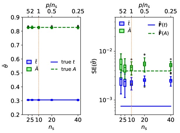
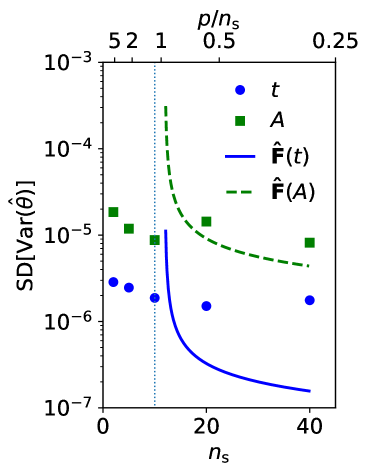
Figure 7: Mean (left), standard error (middle), and standard deviation of the variance (right) of the parameters estimates for $t$ and $A$ from the weak-gravitational-lensing inspired model of Sect. 4.3. The acf distance of Eq. (19) is used. Each simulation size $n_{\textrm{s}}$ corresponds to a number of simulations $n_{\rm s}$ used for the covariance matrix estimate. In the left plot, horizontal lines show the true input values. The middle and right panels display predictions based on the Fisher matrix for the normal likelihood (thin lines). Average values are also displayed in Table 2.

4.4 Experiment: A realistic weak-gravitational lensing model

In this section a realistic weak-lensing power spectrum $C_{\ell}$ derived from a numerical, non-linear model of the large-scale structure and lensing projection is considered [71]. The free parameters are the matter density $\Omega_{\textrm{m}}$ and the power-spectrum normalisation $\sigma_{8}$. One of the main astrophysical contaminants to weak lensing is intrinsic galaxy alignment. Galaxy shapes can be correlated to their surrounding dark-matter environment by gravitational interactions. Alignments can be created by the exertion of torquing moments, or anisotropic stretching and accretion, induced by the surrounding tidal field. Intrinsic alignment creates correlations between galaxy intrinsic galaxy ellipticities (II), and between shear and intrinsic galaxy ellipticities (GI). The former is only important for galaxies very close in redshift, the relative number of which is low in our case of a single broad redshift distribution. Therefore we only account for the GI cross-correlation. Intrinsic alignment can be modeled as a power spectrum $C_{\ell}^{\textrm{GI}}$, which is added to the weak-lensing power spectrum defined in Eq. (4) with an amplitude $A_{\textrm{IA}}$. This results in a new expression for the observed power spectrum from Eq. (7) as

$$C_{\ell,{\rm obs}}=C_{\ell}+A_{\textrm{IA}}C_{\ell}^{\textrm{GI}}+\frac{\sigma_{\varepsilon}^{2}}{\bar{n}}.$$ (27)

In this experiment, we select a fixed value of $A_{\textrm{IA}}=2$, which follows [18].

4.4.1 Data-generating model

As in the previous example the data is composed of the abscissa vector $\bm{x}$ consisting of $n_{\mathrm{d}}=10$ values $x_{i}=\ell_{i}$, equally spaced in $\ell$ between $\ell_{\rm min}=25$ and $\ell_{\rm max}=4,000$. The ordinate vector is the weak-lensing power spectrum, $\bm{y}=\{C_{\ell_{i}}\}$. The covariance matrix is the same as in Sect. 4.3.1; we use the two cases of a Gaussian, and of a Gaussian plus SSC covariance. We chose again a set-up corresponding to a survey similar to Euclid, with observed sky area fraction $f_{\textrm{sky}}=0.363$, galaxy density $\bar{n}=30$ arcmin^-2, and intrinsic ellipticity dispersion $\sigma_{\varepsilon}=0.31$.

4.4.2 Distance function.

We consider the inverse-variance distance Eq. (15), and the acf distance Eq. (19).

$\bm{\mathrm{C}}$	dist.	infer.	$n_{\textrm{s}}$	$\overline{\hat{\Omega}}_{\mathrm{m}}$	SE$(\hat{\Omega}_{\mathrm{m}})$	SD$[$Var$(\hat{\Omega}_{\mathrm{m}})]$	$\overline{\hat{\sigma}}_{8}$	SE$(\hat{\sigma}_{8})$	SD$[$Var$(\hat{\sigma}_{8})]$
G	$\hat{\bm{\mathrm{\Psi}}}$	$\hat{\bm{\mathrm{F}}}$	$\leq p$	-	not computable		-	not computable
			$>p$	-	$0.0032$	$6.0\cdot 10^{-6}$	-	$0.0047$	$1.3\cdot 10^{-5}$
G	diag $\!\hat{\bm{\mathrm{C}}}$	ABC	$\leq p$	$0.3060$	$0.0038$	$6.7\cdot 10^{-6}$	$0.8268$	$0.0056$	$1.4\cdot 10^{-5}$
			$>p$	$0.3057$	$0.0038$	$4.8\cdot 10^{-6}$	$0.8273$	$0.0056$	$1.0\cdot 10^{-5}$
G+SSC	$\hat{\bm{\mathrm{\Psi}}}$	$\hat{\bm{\mathrm{F}}}$	$\leq p$	-	not computable		-	not computable
			$>p$	-	$0.0033$	$6.2\cdot 10^{-6}$	-	$0.0060$	$2.1\cdot 10^{-5}$
G+SSC	diag $\!\hat{\bm{\mathrm{C}}}$	ABC	$\leq p$	$0.3058$	$0.0036$	$5.6\cdot 10^{-6}$	$0.8270$	$0.0061$	$1.6\cdot 10^{-5}$
			$>p$	$0.3067$	$0.0036$	$4.8\cdot 10^{-6}$	$0.8256$	$0.0060$	$1.3\cdot 10^{-5}$
G+SSC	acf	ABC	$\leq p$	$0.3064$	$0.0054$	$1.1\cdot 10^{-5}$	$0.8264$	$0.0077$	$2.6\cdot 10^{-5}$
			$>p$	$0.3062$	$0.0055$	$1.4\cdot 10^{-5}$	$0.8267$	$0.0076$	$2.5\cdot 10^{-5}$

Table 3: Results for the realistic weak-lensing case of Sect.4.4. See Table 2 for details. The true input parameters are $\Omega_{\textrm{m}}=0.306$ and $\sigma_{8}=0.827$.

4.4.3 Experiment details

Each iteration is run with twice the number of points compared to the previous two examples, $M=200$ points, and the initial number of draws from the prior is $M=400$. The convergence criterion is $\delta=0.015$, leading to $41$ iterations on average. With on average $87,000$ draws per run, the overall acceptance rate is $0.1$.

4.4.4 Results

The results are summarized in Table 3, and Fig. 8 shows ABC with the acf distance compared to Fisher-matrix predictions. The results for this weak-lensing case are similar to the quadratic model from Sect. 4.3: the ABC estimates are consistent with the true parameter values. There is no visible dependence on the number of simulations used to compute the covariance matrix, including the case of a singular matrix. We see no adversarial effects on the results from forward-modelling simulations generated with a small number of simulations and under a singular covariance. The main difference to Sect. 4.3 is that SE and SD[Var] for $\hat{\Omega}_{\textrm{m}}$ from ABC is close to the normal likelihood case. The tilt parameter $t$ in Sect. 4.3 had values of SE and SD[Var] significantly larger than the Fisher-matrix predictions, contrary to ${\Omega}_{\textrm{m}}$ in this example.

For the inverse-variance distance the SE of the parameter estimates are very close to the Cramér-Rao bound. The SD[Var] are smaller than in the multivariate normal case. The results from the acf distance are never below the Cramér-Rao case. This indicates that the inverse-variance distance under-estimates the parameter errors due to neglecting the correlation of the observed data vector. This is remedied with the acf distance.

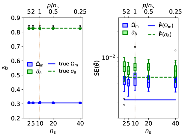
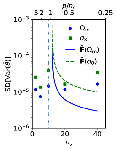
Figure 8: Mean (left), SE (middle), and standard deviation of the variance (SD[Var]; right) of the parameter estimates of $\Omega_{\textrm{m}}$ and $\sigma_{8}$ from the realistic weak-gravitational lensing model of Sect. 4.4. The acf distance of Eq. (19) is used. See Fig. 7 for more details. Numerical values for this setting are shown in Table 3.

5 Conclusions

This paper addresses the challenge of inference in the presence of a singular covariance matrix estimate $\hat{\bm{\mathrm{C}}}$. This can be the case for correlated cosmological observations of the large-scale structure, where the covariance matrix is estimated from $N$-body simulations of the data. If the (typically small since computationally costly) number of simulations $n_{\textrm{s}}$ is less than the (typically large) data dimension $p$, $\hat{\bm{\mathrm{C}}}$ is singular. Likelihood-based inference that requires a precision matrix estimate $\hat{\bm{\mathrm{\Psi}}}$ is not possible in that case. The situation is exacerbated if the covariance matrix also depends on the parameters, and needs to be re-computed for every sampled model [28].

The proposed solution to this challenge is to use an Approximate Bayesian Computation (ABC) framework. To generate model predictions from a multivariate distribution is possible under a singular covariance, and does not require the precision matrix. We consider three examples with increasing complexity: an affine function with diagonal data covariance, a non-linear model with correlated data points inspired by the cosmological weak-gravitational-lensing power spectrum, and a realistic weak-lensing case. The results demonstrate that the proposed ABC approach can recover the input parameter values in these inference problems, with as low a number of simulations as $n_{\textrm{s}}=2$.

Other methods that reduce the number of required simulations to $n_{\textrm{s}}<p$ add an apriori known covariance component, for example shrinkage methods [32, 23] or other hybrid approaches [19]. These methods were tested for $p/n_{\rm s}\leq 12$, while the proposed ABC method can provide reliable parameter constraints for a covariance matrices up to $p/n_{\textrm{s}}=375$.

Data compression has been suggested as a way forward to reduce the requirements on simulations, e.g. Heavens et al. [27], Asgari and Schneider [2], Alsing and Wandelt [1], Charnock et al. [12], Jeffrey et al. [31]. Some of these methods however require the computation of the precision matrix of the un-compressed data. In addition, data compression can potentially lose important information. The proposed ABC approach can work with compressed data, but does not depend on it.

In our simulation study, we found that the estimated parameter means, their standard error, and the standard deviations of their variance do not depend on $n_{\textrm{s}}$. This is in contrast to MCMC sampling, where the standard errors of the estimates display a bias that depends on the number of simulations. The standard errors of the parameter estimates from ABC are in most cases larger than the Cramér-Rao lower bound. Using the predictions from a Hotelling $T^{2}$ distribution, corresponding to an estimated covariance matrix that follows a Wishart distribution, we obtain similar standard errors with ABC.

We introduce a new distance function based on the autocorrelation function (acf) of the data (Eq. 19), which does not use the covariance matrix. The proposed acf distance can account for correlations in the data without relying on a precision matrix. Overall, the proposed ABC framework provides a strategy for inference of correlated observations when it is not possible to run numerous $N$-body simulations to estimate the precision matrix.

Appendix A Parameter covariance matrix for the multivariate normal distribution

A.1 Estimated parameter covariance and its covariance matrix

The $n_{\theta}\times p$ matrix $\bm{\mathrm{M}}$ defined in Eq. (20) has rank $n_{\theta}$. The parameter covariance matrix is the inverse of the Fisher matrix, $\bm{\mathrm{\Phi}}=\bm{\mathrm{F}}^{-1}.$ Since in our case $n_{\theta}=2$, we can analytically take the inverse of $\bm{\mathrm{F}}$ to obtain the parameter variance

$$\textrm{Var}\left(\hat{\theta}_{i}\right)=\Phi_{ii}=\left|\bm{\mathrm{F}}\right|^{-1}F_{jj},$$ (28)

for $(i,j)\in\{(1,2),(2,1)\}$.

An estimator of $\bm{\mathrm{\Phi}}$ can be defined using the estimated precision matrix, $\hat{\bm{\mathrm{\Phi}}}=\left[\bm{\mathrm{M}}^{\textrm{t}}\hat{\Psi}\bm{\mathrm{M}}\right]^{-1}=\left[\bm{\mathrm{M}}^{\textrm{t}}(\hat{\bm{\mathrm{C}}})^{-1}\bm{\mathrm{M}}\right]^{-1}$. Since $\nu\hat{\bm{\mathrm{C}}}\sim{\cal W}_{p}(C,\nu)$, we can apply Theorem 3.3.13 from [21], according to which the estimated parameter covariance matrix follows a Wishart distribution with scale matrix $\bm{\mathrm{\Phi}}=\left[\bm{\mathrm{M}}^{\textrm{t}}{\bm{\mathrm{C}}}^{-1}\bm{\mathrm{M}}\right]^{-1}$ and degrees of freedom $\nu-p+n_{\theta}$: $\left(\nu-p+n_{\theta}\right)\hat{\bm{\mathrm{\Phi}}}\sim{\cal W}_{n_{\theta}}(\bm{\mathrm{\Phi}},\nu-p+n_{\theta})$. Following Table 1, we can write the covariance of the parameter covariance as

$$\mathbb{E}\left(\hat{\Phi}_{ij}-\Phi_{ij}\right)^{2}=\left(\nu-p+n_{\theta}\right)^{-1}\left(\Phi_{ij}^{2}-\Phi_{ii}\Phi_{jj}\right)^{2}$$ (29)

Note that different expression have been obtained in [73] and [66].

The following two sections compute the numerical values of the parameter variances for the affine function (Sect. 4.2), and the weak-lensing inspired example (Sect. 4.3), respectively.

A.2 Standard errors for the affine function

The following expressions correspond to the example of an affine function model $\bm{m}(\bm{\theta})=a\bm{x}+b\bm{1}$, described in Sect. 4.2. With $\theta_{1}=a$ and $\theta_{2}=b$, thus $\partial\bm{m}/\partial\theta_{1}=\bm{x}$ and $\partial\bm{m}/\partial\theta_{2}=\bm{1}$, the Fisher matrix is written as

$$\bm{\mathrm{F}}= \left(\begin{array}[]{cc}\bm{x}^{\rm t}\bm{\mathrm{\Psi}}\bm{x}&\bm{x}^{\rm t}\bm{\mathrm{\Psi}}\bm{1}\\ \bm{x}^{\rm t}\bm{\mathrm{\Psi}}\bm{1}&\bm{1}^{\rm t}\bm{\mathrm{\Psi}}\bm{1}\end{array}\right)\,=\frac{1}{\sigma^{2}}\left(\begin{array}[]{cc}\sum_{i}x_{i}^{2}&\sum_{i}x_{i}\\ \sum_{i}x_{i}&p\end{array}\right).$$ (34)

Using the expected values of the uniformly-distributed $x_{i}$ and their squares, we obtain $F_{11}=(p\Delta^{2})/(12\sigma^{2})$, and $F_{12}=F_{21}=0$. The parameter estimate variances are then

$$\textrm{Var}(\hat{a})=\Phi_{11}=\left({\bm{\mathrm{F}}}^{-1}\right)_{11}=\frac{\sigma^{2}}{p}\frac{12}{\Delta^{2}};\quad\textrm{Var}(\hat{b})=\Phi_{22}=({\bm{\mathrm{F}}}^{-1})_{22}=\frac{\sigma^{2}}{p}.$$ (35)

With $\Delta=200,p=750$, and $\sigma^{2}=5$, the numerical values for the standard errors are SE$(\hat{a})=1/(500\sqrt{2})\approx 0.001414$, SE$(\hat{b})=1/(5\sqrt{6})\approx 0.08165$.

A.3 Standard errors for the weak-lensing inspired example

The following expressions correspond to the example of the weak-lensing inspired example defined in Sect. 4.3. The model function $\bm{m}$ is given by Eqs. (24), (25), and (26). We first compute the derivatives analytically,

$$\frac{\partial\bm{m}}{\partial t}= \frac{a\log 10}{2\times 6.05}(\bm{x}-x_{0}\bm{1})\odot\bm{m}(\bm{\theta});$$

$$\frac{\partial\bm{m}}{\partial A}= \frac{2}{A}\bm{m}(\bm{\theta}),$$ (36)

where $\odot$ denotes Hadamard (element-wide) multiplication. The parameter variances are then obtained by numerically computing the Fisher matrix Eq. (20), and taking the inverse Eq. (28).

A.4 Standard errors for the realistic weak-lensing inspired

For the realistic weak-lensing example (Sect. 4.4), the derivatives of the data vector $y_{\text{sim}}$ with respect to the parameters $\Omega_{\textrm{m}}$ and $\sigma_{8}$ are computed numerically using finite differences. The parameter variances are then obtained following A.3.

References

- Alsing and Wandelt [2018] Alsing, J., Wandelt, B., May 2018. Generalized massive optimal data compression. MNRAS 476, L60–L64.
- Asgari and Schneider [2015] Asgari, M., Schneider, P., Jun. 2015. A new data compression method and its application to cosmic shear analysis. A&A 578, A50.
- Astropy Collaboration et al. [2013] Astropy Collaboration, Robitaille, T. P., Tollerud, E. J., Greenfield, P., Droettboom, M., Bray, et al., Oct. 2013. Astropy: A community Python package for astronomy. A&A 558, A33.
- Barreira et al. [2018a] Barreira, A., Krause, E., Schmidt, F., Oct. 2018a. Accurate cosmic shear errors: do we need ensembles of simulations? JCAP 10, 053.
- Barreira et al. [2018b] Barreira, A., Krause, E., Schmidt, F., Jun 2018b. Complete super-sample lensing covariance in the response approach. JCAP 2018 (6), 015.
- Beaumont [2010] Beaumont, M. A., 2010. Approximate bayesian computation in evolution and ecology. Annual review of ecology, evolution, and systematics 41, 379–406.
- Beaumont et al. [2009] Beaumont, M. A., Cornuet, J.-M., Marin, J.-M., Robert, C. P., 2009. Adaptive approximate Bayesian computation. Biometrika 96 (4), 983 – 990.
- Beaumont et al. [2002] Beaumont, M. A., Zhang, W., Balding, D. J., 2002. Approximate Bayesian computation in population genetics. Genetics 162, 2025 – 2035.
- Bonassi and West [2015] Bonassi, F. V., West, M., 2015. Sequential monte carlo with adaptive weights for approximate bayesian computation. Bayesian Analysis 1 (1), 1–19.
- Bunn [1995] Bunn, E. F., Jan. 1995. Statistical Analysis of Cosmic Microwave Background Anisotropy. Ph.D. Thesis.
-
Carpenter et al. [2017]
Carpenter, B., Gelman, A., Hoffman, M., et al., 2017. Stan: A probabilistic
programming language. Journal of Statistical Software, Articles 76 (1),
1–32.
URL https://www.jstatsoft.org/v076/i01 - Charnock et al. [2018] Charnock, T., Lavaux, G., Wandelt, B. D., Apr. 2018. Automatic physical inference with information maximizing neural networks. Phys. Rev. D97 (8), 083004.
- Chisari et al. [2019] Chisari, N. E., Mead, A. J., Joudaki, S., et al., Jun 2019. Modelling baryonic feedback for survey cosmology. The Open Journal of Astrophysics 2 (1), 4.
- Cook and Forzani [2011] Cook, R., Forzani, L., 01 2011. On the mean and variance of the generalized inverse of a singular wishart matrix. Electronic Journal of Statistics 5.
- Dalmasso et al. [2020] Dalmasso, N., Pospisil, T., Lee, A. B., et al., Jan. 2020. Conditional density estimation tools in python and R with applications to photometric redshifts and likelihood-free cosmological inference. Astronomy and Computing 30, 100362.
- Eisenstein and Hu [1998] Eisenstein, D. J., Hu, W., Mar. 1998. Baryonic Features in the Matter Transfer Function. ApJ 496, 605.
- Euclid Collaboration et al. [2020] Euclid Collaboration, Blanchard, A., et al., Oct. 2020. Euclid preparation. VII. Forecast validation for Euclid cosmological probes. A&A 642, A191.
- Fortuna et al. [2021] Fortuna, M. C., Hoekstra, H., Joachimi, B., et al., Feb. 2021. The halo model as a versatile tool to predict intrinsic alignments. MNRAS 501 (2), 2983–3002.
- Friedrich and Eifler [2018] Friedrich, O., Eifler, T., Jan. 2018. Precision matrix expansion - efficient use of numerical simulations in estimating errors on cosmological parameters. MNRAS 473 (3), 4150–4163.
- Friedrich et al. [2016] Friedrich, O., Seitz, S., Eifler, T. F., Gruen, D., Mar. 2016. Performance of internal covariance estimators for cosmic shear correlation functions. MNRAS 456, 2662–2680.
-
Gupta and Nagar [1999]
Gupta, A., Nagar, D., 1999. Matrix Variate Distributions. Monographs and
Surveys in Pure and Applied Mathematics. Taylor & Francis.
URL https://books.google.fr/books?id=PQOYnT7P1loC - Hahn et al. [2019] Hahn, C., Beutler, F., Sinha, M., Berlind, A., Ho, S., Hogg, D. W., May 2019. Likelihood non-Gaussianity in large-scale structure analyses. MNRAS 485 (2), 2956–2969.
- Hall and Taylor [2019] Hall, A., Taylor, A., Feb. 2019. A Bayesian method for combining theoretical and simulated covariance matrices for large-scale structure surveys. MNRAS 483 (1), 189–207.
-
Hamimeche and Lewis [2009]
Hamimeche, S., Lewis, A., Apr 2009. Properties and use of CMB power spectrum
likelihoods. Phys. Rev. D 79, 083012.
URL https://link.aps.org/doi/10.1103/PhysRevD.79.083012 - Harnois-Déraps et al. [2018] Harnois-Déraps, J., Amon, A., Choi, A., et al., Nov. 2018. Cosmological simulations for combined-probe analyses: covariance and neighbour-exclusion bias. MNRAS 481 (1), 1337–1367.
- Hartlap et al. [2007] Hartlap, J., Simon, P., Schneider, P., Mar. 2007. Why your model parameter confidences might be too optimistic. Unbiased estimation of the inverse covariance matrix. A&A 464, 399–404.
- Heavens et al. [2000] Heavens, A. F., Jimenez, R., Lahav, O., Oct. 2000. Massive lossless data compression and multiple parameter estimation from galaxy spectra. MNRAS 317, 965–972.
- Heavens et al. [2017] Heavens, A. F., Sellentin, E., de Mijolla, D., Vianello, A., Dec. 2017. Massive data compression for parameter-dependent covariance matrices. MNRAS 472, 4244–4250.
-
Hotelling [1931]
Hotelling, H., 08 1931. The generalization of student’s ratio. Ann. Math.
Statist. 2 (3), 360–378.
URL https://doi.org/10.1214/aoms/1177732979 - Ishida et al. [2015] Ishida, E. E. O., Vitenti, S. D. P., Penna-Lima, M., Cisewski, J., et al., Nov. 2015. COSMOABC: Likelihood-free inference via Population Monte Carlo Approximate Bayesian Computation. Astronomy and Computing 13, 1–11.
- Jeffrey et al. [2021] Jeffrey, N., Alsing, J., Lanusse, F., Feb. 2021. Likelihood-free inference with neural compression of DES SV weak lensing map statistics. MNRAS 501 (1), 954–969.
- Joachimi [2017] Joachimi, B., Mar. 2017. Non-linear shrinkage estimation of large-scale structure covariance. MNRAS 466, L83–L87.
- Joachimi et al. [2015] Joachimi, B., Cacciato, M., Kitching, T. D., et al., Nov. 2015. Galaxy Alignments: An Overview. SSR 193, 1–65.
- Joeveer and Einasto [1978] Joeveer, M., Einasto, J., Jan. 1978. Has the Universe the Cell Structure? In: Longair, M. S., Einasto, J. (Eds.), Large Scale Structures in the Universe. Vol. 79. p. 241.
-
Jones et al. [2001–]
Jones, E., Oliphant, T., Peterson, P., et al., 2001–. SciPy: Open source
scientific tools for Python.
URL http://www.scipy.org/ - Joudaki et al. [2017] Joudaki, S., Blake, C., Heymans, C., et al., Feb. 2017. CFHTLenS revisited: assessing concordance with Planck including astrophysical systematics. MNRAS 465 (2), 2033–2052.
- Kacprzak et al. [2020] Kacprzak, T., Herbel, J., Nicola, A., et al., Apr. 2020. Monte Carlo Control Loops for cosmic shear cosmology with DES Year 1. Phys. Rev. D101 (8), 082003.
- Kaiser [1992] Kaiser, N., Apr. 1992. Weak gravitational lensing of distant galaxies. ApJ 388, 272–286.
- Kaiser [1998] Kaiser, N., May 1998. Weak Lensing and Cosmology. ApJ 498, 26–42.
- Kayo and Takada [2013] Kayo, I., Takada, M., Jun. 2013. Cosmological parameters from weak lensing power spectrum and bispectrum tomography: including the non-Gaussian errors. arXiv:1306.4684.
- Kilbinger et al. [2009] Kilbinger, M., Benabed, K., Guy, et al., 2009. Dark-energy constraints and correlations with systematics from CFHTLS weak lensing, SNLS supernovae Ia and WMAP5. A&A 497, 677–688.
- Kilbinger et al. [2017] Kilbinger, M., Heymans, C., Asgari, M., et al., 2017. Precision calculations of the cosmic shear power spectrum projection. MNRAS 472, 2126–2141.
- Kitching et al. [2017] Kitching, T. D., Alsing, J., Heavens, A. F., Jimenez, R., McEwen, J. D., Verde, L., Aug. 2017. The limits of cosmic shear. MNRAS 469, 2737–2749.
- Krause et al. [2017] Krause, E., Eifler, T. F., Zuntz, J., et al., Jun. 2017. Dark Energy Survey Year 1 Results: Multi-Probe Methodology and Simulated Likelihood Analyses. arXiv e-prints, arXiv:1706.09359.
- Laureijs et al. [2011] Laureijs, R., Amiaux, J., Arduini, S., et al., Oct. 2011. Euclid Definition Study Report. arXiv:1110.3193.
- Limber [1953] Limber, D. N., Jan. 1953. The Analysis of Counts of the Extragalactic Nebulae in Terms of a Fluctuating Density Field. ApJ 117, 134–+.
- Lin and Kilbinger [2015] Lin, C.-A., Kilbinger, M., 2015. A new model to predict weak-lensing peak counts. II. Parameter constraint strategies. A&A 583, A70.
- Lin et al. [2016] Lin, C.-A., Kilbinger, M., Pires, S., 2016. A new model to predict weak-lensing peak counts III. Filtering technique comparisons. A&A 593, A88.
- Lin et al. [2020] Lin, C.-H., Harnois-Déraps, J., Eifler, T., Pospisil, T., Mandelbaum, R., Lee, A. B., Singh, S., LSST Dark Energy Science Collaboration, Dec. 2020. Non-Gaussianity in the weak lensing correlation function likelihood - implications for cosmological parameter biases. MNRAS 499 (2), 2977–2993.
- LSST Science Collaboration et al. [2009] LSST Science Collaboration, Abell, et al., Dec. 2009. LSST Science Book, Version 2.0. arXiv:0912.0201.
- Mardia et al. [1979a] Mardia, K. V., Kent, J. T., Bibby, J. M., 1979a. Multivariate Analysis, 1st Edition. Academic Press.
-
Mardia et al. [1979b]
Mardia, K. V., Kent, J. T., Bibby, J. M., 1979b. Multivariate
analysis / K.V. Mardia, J.T. Kent, J.M. Bibby. Academic Press London ; New
York.
URL http://www.loc.gov/catdir/toc/els031/79040922.html - Marin et al. [2011] Marin, J.-M., Pudlo, P., Robert, C. P., Ryder, R., Jan. 2011. Approximate Bayesian Computational methods. arXiv:1101.0955.
- Moral et al. [2011] Moral, P. D., Doucet, A., Jasra, A., 2011. An adaptive sequential Monte Carlo method for approximate Bayesian computation. Statistics and Computing 22 (5), 1009–1020.
-
Olkin and Roy [1954]
Olkin, I., Roy, S. N., 06 1954. On multivariate distribution theory. Ann. Math.
Statist. 25 (2), 329–339.
URL https://doi.org/10.1214/aoms/1177728789 - Peebles [1980] Peebles, P. J. E., 1980. The Large-Scale Structure of the Universe. Princeton University Press.
- Percival et al. [2014] Percival, W. J., Ross, A. J., Sánchez, A. G., et al., Apr. 2014. The clustering of Galaxies in the SDSS-III Baryon Oscillation Spectroscopic Survey: including covariance matrix errors. MNRAS 439, 2531–2541.
- Price-Whelan et al. [2018] Price-Whelan, A. M., Sipőcz, B. M., Günther, H. M., et al., Sep. 2018. The Astropy Project: Building an Open-science Project and Status of the v2.0 Core Package. AJ 156, 123.
- Pritchard et al. [1999] Pritchard, J. K., Seielstad, M. T., Perez-Lezaun, A., 1999. Population growth of human Y chromosomes: A study of Y chromosome microsatellites. Molecular Biology and Evolution 16 (12), 1791 – 1798.
- Riddell et al. [2021] Riddell, A., Hartikainen, A., Carter, M., Mar. 2021. pystan (3.0.0). PyPI.
-
Rosen [1988]
Rosen, D. V., 1988. Moments for matrix normal variables. Statistics 19 (4),
575–583.
URL https://doi.org/10.1080/02331888808802132 - Scaramella et al. [2021] Scaramella, R., Amiaux, J., Mellier, Y., et al., Aug. 2021. Euclid preparation: I. The Euclid Wide Survey. arXiv:2108.01201.
- Schneider et al. [2002] Schneider, P., Van Waerbeke, L., Kilbinger, M., Mellier, Y., 2002. Analysis of two-point statistics of cosmic shear: I. Estimators and covariances. A&A 396, 1–19.
- Seabold and Perktold [2010] Seabold, S., Perktold, J., 2010. statsmodels: Econometric and statistical modeling with python. In: 9th Python in Science Conference.
- Sellentin and Heavens [2016] Sellentin, E., Heavens, A. F., Feb. 2016. Parameter inference with estimated covariance matrices. MNRAS 456, L132–L136.
- Sellentin and Heavens [2017] Sellentin, E., Heavens, A. F., Feb. 2017. Quantifying lost information due to covariance matrix estimation in parameter inference. MNRAS 464 (4), 4658–4665.
- Sellentin and Starck [2019] Sellentin, E., Starck, J.-L., Aug 2019. Debiasing inference with approximate covariance matrices and other unidentified biases. JCAP2019 (8), 021.
- Simon et al. [2015] Simon, P., Semboloni, E., van Waerbeke, L., et al., 2015. CFHTLenS: a Gaussian likelihood is a sufficient approximation for a cosmological analysis of third-order cosmic shear statistics. MNRAS 449, 1505–1525.
- Siskind [1972] Siskind, V., 1972. Second moments of inverse wishart-matrix elements. Biometrika 59, 690–691.
- Sisson et al. [2007] Sisson, S. A., Fan, Y., Tanaka, M. M., 2007. Sequential Monte Carlo without likelihoods. Proceedings of the National Academy of Science 104 (6), 1760 – 1765.
- Takahashi et al. [2012] Takahashi, R., Sato, M., Nishimichi, T., Taruya, A., Oguri, M., Dec. 2012. Revising the Halofit Model for the Nonlinear Matter Power Spectrum. ApJ 761, 152.
- Tavaré et al. [1997] Tavaré, S., Balding, D. J., Griffiths, R., Donnelly, P., 1997. Inferring coalescence times from DNA sequence data. Genetics 145, 505 – 518.
- Taylor and Joachimi [2014] Taylor, A., Joachimi, B., Aug. 2014. Estimating cosmological parameter covariance. MNRAS 442, 2728–2738.
- Taylor et al. [2013] Taylor, A., Joachimi, B., Kitching, T., Jul. 2013. Putting the precision in precision cosmology: How accurate should your data covariance matrix be? MNRAS 432, 1928–1946.
- Tegmark et al. [1997] Tegmark, M., Taylor, A., Heavens, A., 1997. Karhunen-Loève Eigenvalue Problems in Cosmology: How Should We Tackle Large Data Sets? ApJ 480, 22.
- Zel’Dovich [1970] Zel’Dovich, Y. B., Mar. 1970. Reprint of 1970A&A…..5…84Z. Gravitational instability: an approximate theory for large density perturbations. A&A 500, 13–18.