On the existence of holomorphic curves in compact quotients of $\mathrm{SL}(2,\mathbb{C})$

Abstract.

We prove the existence of a pair $(\Sigma,\,\Gamma)$, where $\Sigma$ is a compact Riemann surface with $\text{genus}(\Sigma)\,\geq\,2$, and $\Gamma\,\subset\,{\rm SL}(2,\mathbb{C})$ is a cocompact lattice, such that there is a generically injective holomorphic map $\Sigma\,\longrightarrow\,{\rm SL}(2,\mathbb{C})/\Gamma$. This gives an affirmative answer to a question raised by Huckleberry and Winkelmann [HW] and by Ghys [Gh].

1. Introduction

Compact complex manifolds with holomorphically trivial tangent bundle are known to be biholomorphic to a quotient of a complex Lie group $G$ by a discrete cocompact subgroup $\Gamma$ [Wa]. These manifolds, also known as parallelizable complex manifolds, are Kähler if and only if the Lie group $G$ is abelian (in which case the manifold is a compact complex torus).

Whenever $G$ is a semi-simple Lie group, and $\Gamma\,\subset\,G$ is a cocompact lattice, a theorem of Huckleberry and Margulis [HM] says that $G/\Gamma$ does not admit any complex analytic hypersurface. In particular, the algebraic dimension of $G/\Gamma$ is zero, meaning $G/\Gamma$ does not admit any nonconstant meromorphic function.

An important class of examples consists of compact quotients of $G\,=\,\text{SL}(2,\mathbb{C})$ by cocompact Kleinian subgroups $\Gamma\,\subset\,\text{SL}(2,\mathbb{C})$. Since $\text{PSL}(2,\mathbb{C})$ is the group of orientation preserving isometries of the hyperbolic $3$-space $\mathbb{H}^{3}$, the compact quotient $\text{SL}(2,\mathbb{C})/\Gamma$ is an unramified double cover of the $\text{SO}(3,\mathbb{R})$-bundle of oriented orthonormal frames of the compact hyperbolic $3$-manifold $\mathbb{H}^{3}/\Gamma$. While the embedding of $\Gamma$ into $\text{SL}(2,\mathbb{C})$ is known to be rigid by Mostow’s Theorem, the flexibility of the complex structure of $\text{SL}(2,\mathbb{C})/\Gamma$ was discovered by Ghys [Gh] where he showed that the corresponding Kuranishi space has positive dimension for all $\Gamma$ with positive first Betti number. The corresponding compact hyperbolic $3$-manifolds can be constructed using Thurston’s hyperbolisation Theorem (see, for instance, [Th] and [Gh, Lemme 6.2] for constructions of compact hyperbolic $3$-manifolds with prescribed rational cohomology ring). Nevertheless, much of the interplay between the geometry of the compact hyperbolic $3$-manifold $\mathbb{H}^{3}/\Gamma$ and the complex structure of its oriented orthonormal frame bundle $\text{PSL}(2,\mathbb{C})/\Gamma$ remains to be explored.

In course of his studies of the deformation space of the complex structures of $\text{SL}(2,\mathbb{C})/\Gamma$ Ghys [Gh] encountered a problem previously raised by Huckleberry and Winkelmann [HW] which would generalize the Huckleberry-Margulis Theorem [HM] to holomorphic curves: Does there exist a compact 3-manifold $\text{SL}(2,\mathbb{C})/\Gamma$ admitting a compact holomorphic curve of genus $g\geq 2$? Note that the case of elliptic curves covered by one-parameters groups in $\text{SL}(2,\mathbb{C})$ are well-known to exist in certain quotients $\text{SL}(2,\mathbb{C})/\Gamma$.

In this paper we give an affirmative answer to this open question following a strategy due to Ghys, see [BDHH, CDHeL]. We construct on the trivial holomorphic bundle of rank two over a Riemann surfaces $\Sigma$ an irreducible holomorphic $\text{SL}(2,\mathbb{C})$-connection such that the image of the corresponding monodromy homomorphism lies in a cocompact lattice $\Gamma$ in $\text{SL}(2,\mathbb{C})$. The parallel frame of this connection then gives rise to a holomorphic map from $\Sigma$ into the quotient $\text{SL}(2,\mathbb{C})/\Gamma$ which, due to the irreducibility of the connection, does not factor through any elliptic curve. A first step towards realizing Ghys’ strategy was previously made in [BDHH] where holomorphic connections with (real) Fuchsian monodromy were constructed. In this paper we first show that every irreducible $\text{SL}(2,\mathbb{R})$-representation with sufficient many symmetries can be realized as the monodromy of a holomorphic $\text{SL}(2,\mathbb{C})$-connection. Then an example of such a symmetric representation contained in a cocompact lattice $\Gamma$ in $\text{SL}(2,\mathbb{C})$ is given. We end with an outlook on the relationship between holomorphic curves in SL$(2,\mathbb{C})/\Gamma$ and surfaces of constant mean curvature $H\,=\,1$ in the hyperbolic 3-space.

2. Statements of the main theorems and strategy of proof

Let $\Gamma\,\subset\,\operatorname{SL}(2,\mathbb{C})$ be a cocompact lattice and consider the compact complex $3$-manifold $N\,=\,\operatorname{SL}(2,\mathbb{C})/\Gamma$. This three manifold can be viewed as the double covering of the $\mathrm{SO}(3)$-frame bundle of the corresponding hyperbolic 3-orbifold $\mathbb{H}^{3}/\Gamma$ and it is called the unitary frame bundle. Let $\Sigma$ be a Riemann surface of genus $g\,\geq\,2$, fix a base point $x_{0}\,\in\,\Sigma$ and consider an irreducible representation

$$\rho_{\Sigma}\,\colon\,\pi_{1}(\Sigma,\,x_{0})\,\longrightarrow\,\Gamma\,\subset\,\operatorname{SL}(2,\mathbb{C}).$$

Following an idea of Ghys, we aim at realizing such a representation $\rho_{\Sigma}$ as the monodromy representation of a holomorphic flat connection $\nabla$ on the trivial holomorphic $\mathbb{C}^{2}$-bundle over $\Sigma$. Then the corresponding parallel frame $\Psi\colon\Sigma\rightarrow\operatorname{SL}(2,\mathbb{C}),$ with $\Psi(x_{0})=$ Id induces a well-defined holomorphic map $f_{\rho_{\Sigma}}$ from $\Sigma$ into $N$ (with monodromy representation $\rho_{\Sigma}$). The map $f_{\rho_{\Sigma}}$ does not factor through an elliptic curve since $\rho_{\Sigma}$ is irreducible.

In the following we impose various symmetries on $\Sigma$ and $\rho_{\Sigma}$. Let $\Sigma$ be the covering of $\mathbb{C}P^{1}$ of degree $g+1$ defined by the equation

$$y^{g+1}\,=\,\frac{(z-p_{1})(z-p_{2})}{(z-p_{3})(z-p_{4})},$$ (2.1)

where

$$p_{1}\,=\,e^{i\varphi},\quad p_{2}\,=\,-e^{-i\varphi},\quad p_{3}\,=\,-e^{i\varphi},\quad p_{4}\,=\,e^{-i\varphi}$$ (2.2)

with $\varphi\,\in\,(0,\,\pi/2)$, i.e., $\Sigma$ is totally branched over $p_{1},\,p_{2},\,p_{3},\,p_{4}$. The representations $\rho_{\Sigma}\,=\,\widehat{\rho}$ we consider are compatible with the covering, i.e., it is induced by the monodromy representation $\rho$ of a particular rank $2$ logarithmic connection $\nabla$ (described in Section 3.1) over the 4-punctured sphere

$$S_{4}\,:=\,\mathbb{C}P^{1}\setminus\{p_{1},\,\dots,\,p_{4}\}.$$ (2.3)

Fix a base point $s_{0}\,\in\,S_{4}$, and let $\gamma_{p_{j}}\,\in\,\pi_{1}(S_{4},\,s_{0})$ be the curve that goes around $p_{j}$ anti-clockwise for $j=1,...,4$, such that $\gamma_{p_{4}}\gamma_{p_{3}}\gamma_{p_{2}}\gamma_{p_{1}}\,=\,1$ (see Section 3.2). Let $M_{j}$ denote the monodromy of $\nabla$ along $\gamma_{p_{j}}$. Then $\rho$ is assumed to satisfy the following RSR condition.

Definition 2.1.

An irreducible representation $\rho\,\colon\,\pi_{1}(S_{4},\,s_{0})\,\longrightarrow\,\operatorname{SL}(2,\mathbb{C})$ is called RSR-representation if it has the following three properties:

• Real:  $\rho$ takes values in $\operatorname{SL}(2,\mathbb{R})$ and

  $$x\,=\,\operatorname{tr}(M_{1}M_{2})\,<\,-2,\ \,y\,=\,\operatorname{tr}(M_{2}M_{3})\,<\,-2,\ \,z\,=\,\operatorname{tr}(M_{1}M_{3})\,<\,-2,$$

  where $M_{j}\,=\,\rho(\gamma_{p_{j}})$.

• Symmetric:  the four monodromies $M_{1},\,\cdots,\,M_{4}$ lie in the same conjugacy class determined by $\text{diag}(e^{2\pi i\widetilde{r}},\,e^{-2\pi i\widetilde{r}})$ for some $\widetilde{r}\,\in\,(\tfrac{1}{4},\,\tfrac{1}{2})$.

• Rectangular:  $\text{tr}(M_{1}M_{3})\,=\,\text{tr}(M_{2}M_{4})$.

Every $\rho\,\in\,{\rm Hom}(\pi_{1}(S_{4},\,s_{0}),\,\operatorname{SL}(2,\mathbb{C}))$ such that $\rho(\gamma_{p_{j}})^{k}\,=\,1$ for all $j=1,\,...,\,4,$ for some integer $k\,>\,0$, lifts to a representation of $\pi_{1}(\Sigma,\,x_{0})$ for the Riemann surface in (2.1) of suitable genus $g$, see Lemma 3.16 for the details. This motivates the definition of the genus of a RSR-representation, see also [BDHH, Section 3].

Definition 2.2.

Let $\rho$ be a RSR-representation such that one (and hence all, as they have same conjugacy class) of $M_{1},\,\cdots,\,M_{4}$ have order $k\,\in\,\mathbb{N}.$ Then, the genus of $\rho$ is $k-1,$ if $k$ is odd, and it is $\tfrac{k}{2}-1$ if $k$ is even.

Since the symmetries are analogous to those of the Lawson minimal surfaces of genus $g$, we define:

Definition 2.3.

Any homomorphism $\widehat{\rho}\,:\,\pi_{1}(\Sigma,\,x_{0})\,\longrightarrow\,\operatorname{SL}(2,\mathbb{R})$ induced by some RSR-representation $\rho$ (defined in (2.1)) is called real Lawson-symmetric (RL).

Our main theorem is the following.

Theorem 2.4 (Main Theorem).

Let $\rho$ be a RSR-representation of genus $g$, and let $\Gamma$ be a compatible cocompact lattice in ${\rm SL}(2,\mathbb{C})$, meaning $\Gamma$ contains the image of the corresponding RL-representation $\widehat{\rho}$. Then there exists a genus g Riemann surface $\Sigma$ of the form (2.1) and a holomorphic map from $\Sigma$ to the compact complex 3-manifold SL$(2,\mathbb{C})/\Gamma$. Moreover, the holomorphic map does not factor through a torus.

Remark 2.5.

The techniques presented in this paper produce in fact infinitely many holomorphic maps from Riemann surfaces $\Sigma^{n},$ $n\in\mathbb{N},$ of the same genus into $\operatorname{SL}(2,\mathbb{C})/\Gamma$ inducing the same RL-representation $\widehat{\rho}.$ To enhance clarity we discuss here only the simplest case arising from grafting once.

Remark 2.6.

The assumption of the theorem is for example fulfilled if the 3-manifold $\mathbb{H}^{3}/\Gamma$ contains a totally geodesic surface of genus $g\geq 2$ with enough symmetries such that the induced monodromy representation $\widehat{\rho}$ is RL. Note that in the example we give below, the representation $\widehat{\rho}$ is not Fuchsian.

We prove the following (see Theorem 6.1):

Theorem 2.7.

Let $\Gamma$ be the cocompact lattice in $\mathbb{H}^{3}$ given by the dodecahedron tiling $\{5,3,4\}$ of the hyperbolic 3-space. Then there exist a holomorphic curve of genus $4$ in the compact 3-manifold SL$(2,\mathbb{C})/\Gamma.$

Remark 2.8.

The RSR-representation $\rho$ is obtained from the pentagon tiling of $\mathbb{H}^{2}\subset\mathbb{H}^{3}$ which can be extended to the dodecahedron tiling of $\mathbb{H}^{3}.$ The genus of the RSR-representation is 4. The holomorphic map obtained from this example has 4 simple branch points and by Riemann-Hurwitz it cannot factor through a lower genus surface.

The symmetry assumptions in Theorem 2.4 ensure that the moduli space $\mathcal{M}_{\mathbb{R},sym}(\Sigma)$ of compatible equivariant $\operatorname{SL}(2,\mathbb{R})$-representations, which contains $\rho$, is only (real) $1$-dimensional. Moreover, the compatible Riemann surface structures on $\Sigma$ are determined by rectangular tori $T^{2}_{\tau}\,=\,\mathbb{C}/\mathbb{Z}\oplus i\tau\mathbb{Z}$ for $\tau\,\in\,\mathbb{R}_{>0}$ with one puncture $[0]\,\in\,T^{2}_{\tau}$ given by an appropriate quotient of a Hitchin cover of $\Sigma$. The corresponding flat connections and their representations can therefore be investigated on $T^{2}_{\tau}$ instead of $\Sigma$. The details of the setup are explained in Section 3. To obtain a holomorphic map into $\operatorname{SL}(2,\mathbb{C})/\Gamma$ we show that every element of $\mathcal{M}_{\mathbb{R}}^{r}(T^{2}_{\tau})\cong\mathcal{M}_{\mathbb{R},sym}(\Sigma)$ can be realized as the monodromy representation of a logarithmic connection $\nabla^{H}$ on a specific rank 2 parabolic bundle $H$. Then, this connection over $T^{2}_{\tau}$ is shown to lift to a holomorphic connection on $\mathcal{O}^{\oplus 2}$ over the Riemann surface $\Sigma$ with induced RL-monodromy $\widehat{\rho}.$

In a first step we therefore construct a logarithmic connection $\nabla^{H}(\tau)$ with $\operatorname{SL}(2,\mathbb{R})$-monodromy for every punctured torus $T^{2}_{\tau}\setminus\{o\}$, compare with Theorem 5.3, with the prescribed parabolic structure $H$. This theorem is of independent interest and it is proven in Section 5. The main observation is that grafting, a procedure generating new real projective structures from old ones, changes the induced spin structure on the surface. In this context it is very important to note that we perform grafting not on flat projective bundles, but on their lifts to flat vector bundles which yield the different spin structures. We recall grafting for compact Riemann surfaces in Section 4 together with its straight forward generalization to the case of a 1-punctured torus. Using abelianization on a fixed $T^{2}_{\tau}$ and the fact that (every connected component of) the moduli space $\mathcal{M}_{\mathbb{R}}^{r}$ is diffeomorphic to $\mathbb{R}_{>0}$, we obtain (via the intermediate value theorem) that there exists a holomorphic connection $\nabla^{H}(\tau)$ (on the prescribed parabolic bundle) with real monodromy between the uniformization connection $\nabla^{U}$ of $T^{2}_{\tau}$ and another oper connection $\nabla^{G}$ of $T^{2}_{\tau}$ obtained from a simple-grafting of the uniformization connection of a different Riemann surface $T^{2}_{\tau^{uG}}$.

In a second step, fixing a given representation $\rho\in\mathcal{M}^{r}_{\mathbb{R}}$, we start at an appropriate initial configuration of $\nabla^{U},\nabla^{H}$ and $\nabla^{G}$ and vary the Riemann surface structure $\tau\in\mathbb{R}_{>0}$ of $T^{2}_{\tau}$. We show in Lemma 4.7 and Lemma 4.8 that both connections $\nabla^{U}(\tau)$ and $\nabla^{G}(\tau)$ sweep out the 1-dimensional moduli space of real representations $\mathcal{M}_{\mathbb{R}}^{r}$ (which contains $\rho$). Moreover, $\mathcal{M}_{\mathbb{R}}^{r}$ is an ordered space and the ordering between the three connections $\nabla^{U}$, $\nabla^{H}$ and $\nabla^{G}$ is preserved through a continuous deformation. Since furthermore the Riemann Hilbert mapping is a local diffeomorphism on the 1-punctured torus, see Lemma 5.7, the dependence of $\nabla^{H}(\tau)$ in $\tau$ can be chosen to be continuous. Up to technicalities (which are taken care of), due to the fact that $\tau$ is not necessarily a global coordinate on the submanifold $\mathcal{M}^{r}_{\mathbb{R}}\subset\mathcal{M}_{1,1}^{r},$ the connection $\nabla^{H}(\tau)$ must also sweep out the moduli space $\mathcal{M}^{r}_{\mathbb{R}}$. In particular, there exists a value $\tau_{0}$ such that the monodromy representation of $\nabla^{H}(\tau_{0})$ is the prescribed representation $\rho\in\mathcal{M}^{r}_{\mathbb{R}}$. By replacing $\nabla^{U}(\tau)$ and $\nabla^{G}(\tau)$ with multiple graftings (which differ by a simple-grafting), our arguments show that for every $\rho\in\mathcal{M}_{\mathbb{R}}^{r}$ there exist infinitely many different $\tau_{n}\in\mathbb{R}_{>0},$ $n\in\mathbb{N}$, with holomorphic connections $\nabla^{H}(\tau_{n})$ having the same monodromy $\rho.$ To explain Remark 2.5, note that the Riemann surface structures of the tori $T^{2}_{\tau_{n}}$ and the Riemann surfaces (2.1) both degenerate as $n\to\infty$ and we obtain infinitely many different holomorphic curves in the quotient of $\mathrm{SL}(2,\mathbb{C})$ by the compatible cocompact lattice $\Gamma$.

Theorem 2.4 would worth little if we could not prove the existence of at least one RSR-representation compatible with a cocompact lattice $\Gamma.$ In the last section (Theorem 6.1) we explicitly construct an RSR-representation and show that it is compatible with the cocompact lattice of the dodecahedron $\{5,3,4\}$ tessellation of the hyperbolic 3-space. We expect many more examples by investigating the existence of totally geodesic surfaces inside compact hyperbolic $3$-manifold with RSR-monodromy.

3. Abelianization on Symmetric Riemann surfaces

3.1. Logarithmic connections and parabolic bundles

Consider a compact connected Riemann surface $\Sigma$. Its canonical line bundle will be denoted by $K_{\Sigma}$, while ${\mathcal{O}}_{\Sigma}$ will denote the sheaf of holomorphic functions on $\Sigma$. A holomorphic $\rm{SL}(2,\mathbb{C})$–bundle over $\Sigma$ is a rank two holomorphic vector bundle $V\,\longrightarrow\,\Sigma$ such that the determinant line bundle $\det V\,:=\,\bigwedge^{2}V$ is holomorphically trivial.

Let ${\mathbf{D}}\,=\,p_{1}+\ldots+p_{n}$ be an effective reduced divisor, i.e., the points $p_{j}\,\in\,\Sigma$ are pairwise distinct. Denote by ${\overline{\partial}}_{V}$ the Dolbeault operator for a holomorphic $\rm{SL}(2,\mathbb{C})$–bundle $V$ on $\Sigma$; so the kernel of ${\overline{\partial}}_{V}$ defines the sheaf $\mathcal{V}$ of holomorphic sections of $V$. A logarithmic $\rm{SL}(2,\mathbb{C})$–connection $\nabla\,=\,\overline{\partial}_{V}+\partial^{\nabla}$ on $V$ with polar part contained in the divisor $\mathbf{D}$ is a holomorphic differential operator

$$\partial^{\nabla}\,:\,\mathcal{V}\,\longrightarrow\,\mathcal{V}\otimes K_{\Sigma}\otimes{\mathcal{O}}_{\Sigma}({\mathbf{D}})$$

such that

• the Leibniz rule $\partial^{\nabla}(fs)\,=\,f\partial^{\nabla}(s)+s\otimes\partial{f}$ holds for all $s\in\mathcal{V}$ and $f\in{\mathcal{O}}_{\Sigma}$, and

• the induced holomorphic connection on $\det V\,=\,{\mathcal{O}}_{\Sigma}$ coincides with the de Rham differential $d$ on ${\mathcal{O}}_{\Sigma}$.

Note that all logarithmic connections on $\Sigma$ are necessarily flat. At every point $p_{j}$ in the singular divisor ${\mathbf{D}}$ of a logarithmic $\rm{SL}(2,\mathbb{C})$–connection $\nabla$ on $V$, the associated residue

$$\text{Res}_{p_{j}}(\nabla)\,\in\,\text{End}(V_{p_{j}})$$

is tracefree. Let $\rho_{j}$ and $-\rho_{j}$ be the eigenvalues of $\text{Res}_{p_{j}}(\nabla)$; the logarithmic connection $\nabla$ is called non-resonant if $2\rho_{j}\,\notin\,\mathbb{Z}$ for all $j\,=\,1,\,\cdots,\,n$. In the non-resonant case, the local monodromy of $\nabla$ around $p_{j}$ is conjugate to the diagonal matrix with entries $\exp(\pm 2\pi i\rho_{j})$ (see [De, p. 53, Théorème 1.17]).

A parabolic structure $\mathcal{P}$ on a $\rm{SL}(2,\mathbb{C})$–bundle $V$ over the divisor ${\mathbf{D}}$ is defined by a collection of complex lines $L_{j}\,\subset\,V_{p_{j}}$ together with parabolic weights $r_{j}\,\in\,]0,\,\tfrac{1}{2}[$ for all $j\,=\,1,\,\cdots,\,n$. For a parabolic structure $\mathcal{P}$, the divisor ${\mathbf{D}}$ is called the parabolic divisor and $\{L_{j}\}_{j=1}^{n}$ are called the quasiparabolic lines. The parabolic degree of a holomorphic line subbundle $W\,\subset\,V$ is defined to be

$$\text{par-deg}(W)\,:=\,{\rm deg}(W)+\sum_{j=1}^{n}r^{W}_{j}\,,$$

where $r^{W}_{j}\,=\,r_{j}$ if $W_{p_{j}}\,=\,L_{j}$, and $r^{W}_{j}\,=\,-r_{j}$ if $W_{p_{j}}\,\neq\,L_{j}$.

Definition 3.1 ([MS, MY]).

A parabolic structure $\mathcal{P}$ on the $\rm{SL}(2,\mathbb{C})$–bundle $V$ is called stable (respectively, semistable) if $\text{par-deg}(W)\,<\,0$ (respectively, $\text{par-deg}(W)\,\leq\,0$) for every holomorphic line subbundle $W\,\subset\,V$. A semistable parabolic bundle that is not stable is called strictly semistable. A parabolic bundle which is not semistable is called unstable.

Any non-resonant logarithmic $\rm{SL}(2,\mathbb{C})$–connection $\nabla$ on $V$ for which all the residues have their eigenvalues in the interval $(-\tfrac{1}{2},\,\tfrac{1}{2})$ induces a parabolic structure $\mathcal{P}$ on $V$. The parabolic divisor of $\mathcal{P}$ is the singular locus $\mathbf{D}\,=\,p_{1}+\ldots+p_{n}$ of $\nabla$. The parabolic weight at $p_{j}$ is the positive eigenvalue $\rho_{j}$ of $\text{Res}_{p_{j}}(\nabla)$ and the quasiparabolic line at $p_{j}$ is the eigenline for $\rho_{j}$.

A strongly parabolic Higgs field on a parabolic $\rm{SL}(2,\mathbb{C})$–bundle $(V,\,{\mathcal{P}})$ is a holomorphic section

$$\Phi\,\in\,H^{0}(\Sigma,\,\text{End}(V)\otimes K_{\Sigma}\otimes{\mathcal{O}}_{\Sigma}({\mathbf{D}}))$$

such that $\text{tr}(\Phi)\,=\,0$ and

$$\Phi(p_{j})(V_{p_{j}})\,\subset\,L_{j}\otimes(K_{\Sigma}\otimes{\mathcal{O}}_{\Sigma}({\mathbf{D}}))_{p_{j}}$$

for all $j\,=\,1,\,\cdots,\,n$. These conditions imply that $\Phi(p_{j})$ is nilpotent with the quasiparabolic lines $L_{j}\,\subset\,{\rm kernel}(\Phi(p_{j}))$ for all $j=1,...,n$.

Two non-resonant logarithmic $\rm{SL}(2,\mathbb{C})$–connections $\nabla_{1}$ and $\nabla_{2}$ on $V$ with polar part contained in ${\mathbf{D}}\,=\,p_{1}+\ldots+p_{n}$ induce the same parabolic structure on $V$ if and only if $\nabla_{1}-\nabla_{2}$ is a strongly parabolic Higgs field for the parabolic structure given by $\nabla_{1}$ (or equivalently, for the parabolic structure given by $\nabla_{2}$).

A general result of Mehta and Seshadri [MS, p. 226, Theorem 4.1(2)], and Biquard [Biq, p. 246, Théorème 2.5] (see also [Pi, Theorem 3.2.2]) implies that the above construction of associating a parabolic bundle to a logarithmic connection actually produces a bijection between the space of isomorphism classes of irreducible flat ${\rm SU}(2)$–connections on $\Sigma\setminus{\mathbf{D}}$ and the stable parabolic $\rm{SL}(2,\mathbb{C})$–bundles on $(\Sigma,\,{\mathbf{D}})$. As a consequence, every logarithmic connection $\nabla$ on $V$ giving rise to a stable parabolic $\rm{SL}(2,\mathbb{C})$–structure $\mathcal{P}$ admits a unique strongly parabolic Higgs field $\Phi$ on $(V,\,{\mathcal{P}})$ such that the monodromy representation of $\nabla+\Phi$ is unitary.

3.2. Flat $\rm{SL}(2,\mathbb{C})$–connections on the $4$-punctured sphere

Let ${\mathcal{S}}_{4}$ denote the Riemann sphere $\mathbb{C}P^{1}$ with four unordered marked points

$${\mathcal{S}}_{4}\,:=\,(\mathbb{C}P^{1},\,\{p_{1},\,\cdots,\,p_{4}\})\,,$$

with $p_{j}$ as in (2.2) and recall that

$$S_{4}\,=\,\mathbb{C}P^{1}\setminus\{p_{1},\,\cdots,\,p_{4}\}\,$$ (3.1)

is the underlying topological four-punctured sphere. Fix a base point $s_{0}\,\in\,S_{4}$. For every $j=1,\,...,\,4$, consider a simply closed, oriented, and $s_{0}$-based loop $\gamma_{p_{j}}$ going around a single puncture $p_{j}$. The fundamental group $\pi_{1}(S_{4},\,s_{0})$ is generated by these curves $\gamma_{p_{j}}$ with $j=1,\,...,\,4$ and they satisfy the relation $\gamma_{p_{4}}\gamma_{p_{3}}\gamma_{p_{2}}\gamma_{p_{1}}\,=\,1$.

Convention.  For convenience, the composition of loops generating the fundamental group operation is considered to be from right to left, i.e., $\gamma_{2}\gamma_{1}$ denotes the loop obtained by first performing the loop $\gamma_{1}$ and then $\gamma_{2}$.

Every $\operatorname{SL}(2,\mathbb{C})$-representation of $\pi_{1}(S_{4},\,s_{0})$ is determined by the images $M_{j}\,\in\,\operatorname{SL}(2,\mathbb{C})$ of the generators $\gamma_{p_{j}}\,\in\,\pi_{1}(S_{4},\,s_{0})$, for $j=1,\,...,\,4$ and we have

$$M_{4}M_{3}M_{2}M_{1}\,=\,I.$$

We restrict to the symmetric case where

$$\operatorname{tr}(M_{j})\,=\,2\cos(2\pi\widetilde{r}),\;\quad\forall\,\,\,\;j=1,\,...,\,4,$$

with $\widetilde{r}\in(\frac{1}{4},\,\frac{1}{2}).$ We denote by $\mathcal{M}_{0,4}^{\widetilde{r}}$ the space of equivalence classes of $\operatorname{SL}(2,\mathbb{C})$-representation of $\pi_{1}(S_{4},\,s_{0})$ with local monodromy satisfying the above condition at all punctures. This $\mathcal{M}_{0,4}^{\widetilde{r}}$ is identified with the space of flat $\operatorname{SL}(2,\mathbb{C})$-connections on the four-punctured sphere such that all four local monodromies are in the same conjugacy class given by

$${\left(\begin{matrix}e^{-2\pi i\widetilde{r}}&0\\ 0&e^{2\pi i\widetilde{r}}\end{matrix}\right)}\,\in\,{\rm SL}(2,{\mathbb{C}})\,.$$ (3.2)

For $\rho\in\mathcal{M}_{0,4}^{\widetilde{r}}$, we denote by

$$\widetilde{x}\,=\,\operatorname{tr}(M_{2}M_{1}),\,\ \widetilde{y}\,=\,\operatorname{tr}(M_{3}M_{2}),\,\ \widetilde{z}=\operatorname{tr}(M_{3}M_{1})$$

its trace coordinates. They satisfy

$$\widetilde{x}^{2}+\widetilde{y}^{2}+\widetilde{z}^{2}+\widetilde{x}\widetilde{y}\widetilde{z}-2\mu^{2}(\widetilde{x}+\widetilde{y}+\widetilde{z})+4(\mu^{2}-1)+\mu^{4}\,=\,0.$$ (3.3)

The corresponding affine variety is called a (relative) character variety. The following result of characterizing a representation by its image in the corresponding relative character variety is well-known and dates back to Fricke and Klein, see [Go88, BeG].

Lemma 3.2.

Let $(\widetilde{x},\widetilde{y},\widetilde{z})\in\mathbb{C}^{3}$ satisfying equation (3.3) and $(\widetilde{x}-2)(\widetilde{y}-2)(\widetilde{z}-2)\,\neq\,0$. Then, there exist a unique $\rho\in\mathcal{M}_{0,4}^{\widetilde{r}}$ such that $(\widetilde{x},\widetilde{y},\widetilde{z})$ are the trace coordinates of $\rho$.

Moreover, a totally reducible representation is conjugate to a $\mathrm{SU}(2)$-representation if and only if $\widetilde{x},\,\widetilde{y},\,\widetilde{z}\,\in\,[-2,\,2]$, while it is conjugate to an $\operatorname{SL}(2,\mathbb{R})$-representation if $\widetilde{x},\,\widetilde{y},\,\widetilde{z}\,\in\,\mathbb{R}$ are real and at least one of them lying in $\mathbb{R}\setminus[-2,\,2]$.

Remark 3.3.

For the parabolic weight $\widetilde{r}\,\in\,(0,\,\frac{1}{4})$, there is a natural biholomorphic map between the character varieties for $\widetilde{r}$ and $\tfrac{1}{2}-\widetilde{r}$. In fact, this biholomorphism is induced by $M_{k}\,\longmapsto\,-M_{k}$, which gives the identity map in terms of the respective $(\widetilde{x},\,\widetilde{y},\,\widetilde{z})$-trace coordinates. Note that

$$2\text{cos}(2\pi\widetilde{r})\,=\,-2\text{cos}(2\pi(\tfrac{1}{2}-\widetilde{r})),$$

and therefore also equation (3.3) does not change.

3.3. Flat $\rm{SL}(2,\mathbb{C})$–connections on the 1-punctured torus

For $\tau\,\in\,\mathbb{R}_{>0}$ let

$$T_{\tau}^{2}\,:=\,\mathbb{C}/\Gamma,\quad\text{with}\quad\Gamma\,=\,{\mathbb{Z}}+\tau i{\mathbb{Z}}\,\subset\,\mathbb{C}$$ (3.4)

be a rectangular torus. Moreover, let $o\,=\,[0]\,\in\,T_{\tau}^{2}$ and $p_{0}\,:=\,\frac{1+\tau i}{4}\,\in\,T_{\tau}^{2}$ and consider $\pi_{1}(T_{\tau}^{2}\setminus\{o\},\,p_{0})$ the fundamental group of the one-punctured torus $T_{\tau}^{2}\setminus\{o\}$ with basepoint $p_{0}$. This is a free group with two generators $\gamma_{x},\,\gamma_{y}\,\in\,\pi_{1}(T_{\tau}^{2}\setminus\{o\},\,p_{0}),$ where

$$\gamma_{x}\,\colon\,[0,\,1]\,\longrightarrow\,T_{\tau}^{2}\setminus\{o\};\ \,s\,\longmapsto\,s+\frac{1+\tau i}{4}$$ (3.5)

and

$$\gamma_{y}\,\colon\,[0,\,1]\,\longrightarrow\,T_{\tau}^{2}\setminus\{o\};\ \,s\,\longmapsto\,\tau is+\frac{1+\tau i}{4}.$$ (3.6)

The commutator $\gamma_{y}^{-1}\gamma_{x}^{-1}\gamma_{y}\gamma_{x}\,\in\,\pi_{1}(T_{\tau}^{2}\setminus\{o\},\,p_{0})$ corresponds to a simple loop going around the marked point $o$ anti-clockwise.

For $r\in(0,\,\tfrac{1}{2})$ let $\mathcal{M}_{1,1}^{r}$ be the moduli space of flat $\mathrm{SL}(2,\mathbb{C})$-connections on the 1-punctured torus $T^{2}_{\tau}\setminus\{o\}$ with local monodromy around the marked point $o$ lying in the conjugacy class of the matrix

$${\left(\begin{matrix}e^{-2\pi ir}&0\\ 0&e^{2\pi ir}\end{matrix}\right)}\,\in\,{\rm SL}(2,{\mathbb{C}})\,.$$ (3.7)

As for the 4-punctured sphere, the conjugacy class is determined by the value of its trace $2\cos(2\pi r)$, see [Go03]. For an element in $\mathcal{M}_{1,1}^{r}$ let $X,\,Y$ be the monodromies along the curves

$$\gamma_{x},\,\gamma_{y}\,\in\,\pi_{1}(T^{2}_{\tau}\setminus\{0\},\,p_{0})$$

(defined in (3.5) and (3.6)), and let

$$x\,=\,\operatorname{tr}(X),\quad y\,=\,\operatorname{tr}(Y),\quad z\,=\,\operatorname{tr}(YX)$$

be the corresponding trace coordinates satisfying the equation

$$x^{2}+y^{2}+z^{2}-xyz-2-2\cos(2\pi r)\,=\,0\,.$$ (3.8)

The corresponding affine variety is also called the (relative) character variety of the 1-punctured torus. By a result of Fricke, the moduli space $\mathcal{M}_{1,1}^{r}$ is diffeomorphic to the character variety defined in (3.8) by associating to a monodromy representation the traces $x\,=\,\operatorname{tr}(X),\,y\,=\,\operatorname{tr}(Y)$ and $z\,=\,\operatorname{tr}(YX)$ (see, [Go03, Section 2.1]).

Remark 3.4.

For given $x$ and $y$, the equation (3.8) is quadratic in $z$, and hence there are two (possibly equal) solutions of (3.8) in $z$ which we refer to as $z_{1}$ and $z_{2}$. If $r$, $x$ and $y$ are all real, then $z_{1}$ and $z_{2}$ are complex conjugate to each other.

Theorem 3.5 ([Go03]).

For $r\,\in\,(0,\,\tfrac{1}{2})$ fixed, the space of all real points of the character variety defined by (3.8) has 5 connected components: one compact component characterized by the condition $x,\,y,\,z\,\in\,[-2,\,2]$ and four non-compact components (which are all diffeomorphic to each other). The compact component consists of $\mathrm{SU}(2)$-representations, while the non-compact components consist of $\mathrm{SL}(2,\mathbb{R})$-representations.

Remark 3.6.

The non-compact components are interchanged by tensoring with a flat $\mathbb{Z}_{2}$-bundle. These are called sign-change automorphisms by Goldman [Go03].

A map between the character varieties

By [BDHH, Theorem 4.9] (see also [HH]), there exists for every $r\,\in\,(0,\,\tfrac{1}{2})$ a degree 4 birational map between the moduli space $\mathcal{M}^{r}_{1,1}$ of flat $\mathrm{SL}(2,\mathbb{C})$-connections on the one-punctured torus $T^{2}_{\tau}$ (as defined in (3.4)) and the moduli space $\mathcal{M}_{0,4}^{\widetilde{r}}$ of flat $\mathrm{SL}(2,\mathbb{C})$-connections on the four-punctured sphere $S_{4}$ (as defined in (2.3)) with

$$\widetilde{r}\,=\,\tfrac{1+2r}{4}\,\in\,(\tfrac{1}{4},\,\tfrac{1}{2}).$$

On the level of character varieties this map $\mathcal{M}^{r}_{1,1}\longrightarrow\mathcal{M}_{0,4}^{\widetilde{r}}$ is given by

$$(x,\,y,\,z)\,\longmapsto\,(\widetilde{x},\,\widetilde{y},\,\widetilde{z})\,=\,(2-x^{2},\,2-y^{2},\,2-z^{2}).$$ (3.9)

The construction of the above map in [BDHH, Theorem 4.9] uses the rectangular torus $T^{2}_{\tau}$, with $\tau\in\mathbb{R}_{>0},$ being a double cover of $\mathbb{C}P^{1}$ branched over the four points $p_{1},\,\cdots,\,p_{4}$ (defined in (2.2)), i.e., $T^{2}_{\tau}$ is given by

$$y^{2}\,=\,\frac{(z-p_{1})(z-p_{2})}{(z-p_{3})(z-p_{4})}.$$

Define

$${\mathcal{S}}_{4}(\tau)\,:=\,(\mathbb{C}P^{1},\,\{p_{1},\,\cdots,\,p_{4}\})\,,$$ (3.10)

with $p_{j}$ as in (2.2), chosen to define a rectangular torus $T^{2}_{\tau}$, with $\tau\,\in\,\mathbb{R}_{>0}$. Since $T_{\tau}^{2}$ is rectangular, the reflection along one edge

$$\eta\,\colon\,T_{\tau}^{2}\,\longrightarrow\,T_{\tau}^{2},\quad[w]\,\longmapsto\,[\overline{w}],$$ (3.11)

where $w$ is the global coordinate on $\mathbb{C},$ defines a real involution on $T_{\tau}^{2}$.

Remark 3.7.

Since the real involution $\eta$ considered here is different than in [BDHH], we also use slightly different coverings of the 4-punctured sphere, see Lemma 3.16. Nevertheless, the main results in [BDHH] to obtain Fuchsian representations on the holomorphically trivial bundle remain true by analogous arguments.

3.4. Abelianization

Every element in $\mathcal{M}_{1,1}^{r}$ can be represented (meaning it lies in the same smooth gauge class) by a logarithmic flat connection with a simple pole at $o$. Abelianization yields particularly well-behaved coordinates $a,\,\chi\,\in\,\mathbb{C}$ on ${\mathcal{M}}_{1,1}^{r}$ as follows, see also [BDH, Section 4], or [HH]. For $L$ being the $C^{\infty}$-trivial bundle $T_{\tau}^{2}\times{\mathbb{C}}\,\longrightarrow\,T_{\tau}^{2}$ the generic logarithmic connection in $\mathcal{M}_{1,1}^{r}$ is given by

$$\nabla\,=\,\nabla^{a,\chi,r}\,=\,{\left(\begin{matrix}\nabla^{L}&\gamma^{-}_{\chi}\\ \gamma^{+}_{\chi}&\nabla^{L^{*}}\end{matrix}\right)}\,,$$ (3.12)

where

$$\nabla^{L}\,=\,d+adw+\chi d\overline{w}$$ (3.13)

is the flat connection on $L$ for constant $a,\,\chi\in\mathbb{C}$ and $w$ being the global holomorphic coordinate on $T_{\tau}^{2}$ (see [BDH, Section 4]). Moreover, $\nabla^{L^{*}}$ is the dual connection of $\nabla^{L}$, and the induced holomorphic structure (by (3.12)) on $L$ is given by the Dolbeault operator $\overline{\partial}^{0}+\chi d\overline{w}$, where $\overline{\partial}^{0}\,=\,d^{\prime\prime}$ is the $(0,1)$-part of the de Rham differential operator $d$. In this generic case, characterized by $\chi$ not being a half-lattice point of Jac$(T^{2}_{\tau})$, i.e., $L^{2}\neq\mathcal{O}_{T_{\tau}^{2}},$ $\gamma^{+}_{\chi}$ and $\gamma^{-}_{\chi}$ are meromorphic sections with respect to the holomorphic structures given by the Dolbeault operators

$$\overline{\partial}^{0}-2\chi d\overline{w}\quad\text{ and }\quad\overline{\partial}^{0}+2\chi d\overline{w},$$

respectively, with simple poles at $o\,\in\,T^{2}_{\tau}$ and residues determined by the eigenvalue of the local monodromy $r\in(0,\frac{1}{2})$.

In the non-generic case, the underlying rank two holomorphic bundle is a non-trivial extension of a spin bundle $S$ by itself. With respect to the $C^{\infty}$-splitting $S\oplus S^{*}$ the Dolbeaut operator is given by

$$\overline{\partial}^{\nabla}\,=\,{\left(\begin{matrix}\overline{\partial}^{0}+\chi d\overline{w}&d\overline{w}\\ 0&\overline{\partial}^{0}-\chi d\overline{w}\end{matrix}\right)}$$ (3.14)

for a half lattice point $\chi\in$ Jac$(T^{2}_{\tau})$, while the $\partial$-part

$$\partial^{\nabla}\,=\,{\left(\begin{matrix}\partial^{S}&bdw\\ cdw&(\partial^{S})^{*}\end{matrix}\right)}\,$$ (3.15)

is singular at $o$, i.e., $\partial^{S}$ and its dual $(\partial^{S})^{*}$ are line bundle connections singular at $o$ and $b$ is a function singular at $o,$ but $c\in\mathbb{C}^{*}$ is a non-zero constant. Thus, in the non-generic case, the connection takes the form of an (orbifold) oper, compare with (4.1) below.

Remark 3.8.

For given $\nabla$ the holormorphic structure on $L$, denoted by $\chi(\nabla)\in$ Jac$(T^{2}_{\tau})$ by abuse of notation, is only well defined up to taking the dual.

Remark 3.9.

The parabolic weight at the puncture $o$ induced by the logarithmic connection $\nabla$ is given by $r.$ For $\nabla=\nabla^{a,\chi,r}$, where $\chi$ is not a half-lattice point, the parabolic line $l_{o}$ is uniquely determined, up to a holomorphic automorphism of $L\oplus L^{*}$, by the condition that it is neither the line $L_{o}$, nor the line $L^{*}_{o}$ (i.e., the off-diagonal is non-zero). In the non-generic case, the parabolic line is either given by $l_{o}=S_{0}$ and the parabolic bundle is unstable, or the parabolic line is not contained in the unique holomorphic line subbundle of degree 0, and the parabolic bundle is stable.

Note that $o$ is contained in the fix point set of the reflexion $\eta$ in (3.11). Since $r\in(0,\,\frac{1}{2})$ is real, $\eta$ induces a real involution of the corresponding de Rham moduli space

$$\widehat{\eta}\,\colon\,\mathcal{M}_{1,1}^{r}\,\longrightarrow\,\mathcal{M}_{1,1}^{r},\ \quad[\nabla]\,\longmapsto\,[\eta^{*}\overline{\nabla}]$$

and we have

Lemma 3.10.

On the rectangular torus $T_{\tau}^{2}$ the gauge class of a connection $\nabla\,=\,\nabla^{a,\chi,r}$, with $\chi\notin\tfrac{1}{2}\Gamma$, is fixed by the involution $\eta$ if and only if one of the following four conditions holds:

$$\begin{split}&\chi\in\mathbb{R},\;\text{ and }\,\;a\,\in\,\mathbb{R},\\ \text{or }\quad&\chi+k\frac{\pi i}{2}\,\in\,\mathbb{R}\,\;\text{ and }\;a-k\frac{\pi i}{2}\,\in\,\mathbb{R}\;\;\text{for some }\;k\,\in\,\mathbb{Z},\\ \text{or }\quad&\chi\,\in\,i\mathbb{R}\,\;\text{ and }\;a\,\in\,i\mathbb{R},\\ \text{ or }\quad&\chi+k\frac{\pi}{2\tau}\,\in\,i\mathbb{R}\,\;\text{ and }\;a-k\frac{\pi}{2\tau}\,\in\,i\mathbb{R}\;\;\text{for some }\;k\,\in\,\mathbb{Z}.\end{split}$$ (3.16)

Proof.

We have

$$\eta^{*}dw\,=\,d\overline{w}\quad\text{and}\quad\eta^{*}d\overline{w}\,=\,dw.$$

Hence, for $\chi\,\in\,\mathbb{R}$ and $a\,\in\,\mathbb{R}$, the connection $\nabla^{L}$ in (3.13) satisfies the condition

$$\eta^{*}\overline{\nabla^{L}}\,=\,\nabla^{L}.$$

By [HH, BDH] the sections $\gamma^{\pm}_{\chi}$ in (3.12) are unique up to scaling. Moreover, the quadratic residue of

$$\gamma^{+}_{\chi}\gamma^{-}_{\chi}(dw)^{2}$$

is $r^{2}$, and hence this residue determines the conjugacy class of the monodromy of $\nabla$ around the singular point $o\,\in\,T_{\tau}^{2}$. Thus, we obtain constants $c^{+},\,c^{-}$ with

$$\eta^{*}\overline{\gamma^{\pm}_{\chi}dw}\,=\,c^{\pm}\gamma^{\pm}_{\chi}$$

and consequently the two connections $\nabla$ and $\eta^{*}\overline{\nabla}$ are gauge equivalent. The argument for the other $3$ cases in (3.16) works analogously.

Conversely, if the pull-back $\eta^{*}\overline{\nabla}$ is gauge equivalent to $\nabla$ then (by [HH, BDHH]) $\eta^{*}\overline{\nabla}^{L}$ is gauge equivalent to either $\nabla^{L}$ or its dual. This yields that $a$ and $\chi$ must satisfy one of the conditions in (3.16) ∎

For latter purposes, we denote the space of $\eta$-invariant representations by

$$\mathcal{M}_{1,1}^{r,\eta}\,:=\,\{[\nabla]\,\in\,\mathcal{M}_{1,1}^{r}\,\,\mid\,\,\,[\eta^{*}\overline{\nabla}]\,=\,[\nabla]\}.$$

3.5. The hidden symmetries of RSR-representations

Proposition 3.11.

For $\widetilde{r}\,\in\,(\tfrac{1}{4},\,\tfrac{1}{2})$ consider $\widetilde{\rho}\in\mathcal{M}_{0,4}^{\widetilde{r}}$ and let $(\widetilde{x},\,\widetilde{y},\,\widetilde{z})$ be the corresponding trace coordinates satisfying (3.3) and $(\widetilde{x}-2)(\widetilde{y}-2)(\widetilde{z}-2)\,\neq\,0$ (as in Lemma 3.2). Then there exist an element $(x,\,y,\,z)$ in $\mathcal{M}_{1,1}^{r}$, unique up to signs, satisfying (3.8) with $r\,=\,2\widetilde{r}-\frac{1}{2}$ such that

$$\widetilde{x}\,=\,2-x^{2},\quad\widetilde{y}\,=\,2-y^{2},\quad\widetilde{z}\,=\,2-z^{2}.$$ (3.17)

Proof.

As in the proof of Theorem 4.9 in [BDHH], the Klein-Fricke equation (3.3) factors into the product of the Klein-Fricke equation (3.8) for $(x,\,y,\,z)$ and the Klein-Fricke equation (3.8) for $(x,\,y,\,-z)$ when applying (3.17). Hence, for given $(\widetilde{x},\,\widetilde{y},\,\widetilde{z})$ either the corresponding $(x,\,y,\,z)$ or $(x,\,y,\,-z)$ solves equation (3.8). ∎

Remark 3.12.

Proposition 3.11 shows the existence of additional symmetries of representations $\widetilde{\rho}\in\mathcal{M}_{0,4}^{\widetilde{r}}$ on the 4-punctured sphere, see equation (4.19) in [BDHH] or [Go97, $\S~{}6$].

Corollary 3.13.

For $\widetilde{r}\,\in\,(\tfrac{1}{4},\,\tfrac{1}{2})$ let $\rho\in\mathcal{M}_{0,4}^{\widetilde{r}}$ be a RSR-representation. Then $\rho$ corresponds via abelianization to a real representation in $\mathcal{M}_{1,1}^{r},$ with $r\,=\,2\widetilde{r}-\frac{1}{2}$. By abuse of notation we will denote the induced representation in $\mathcal{M}_{1,1}^{r},$ by $\rho$ as well.

Proof.

By Definition 2.1, the image of $\rho$ in the character variety (3.3) is a point $(\widetilde{x},\,\widetilde{y},\,\widetilde{z})$ such that $\widetilde{x}\,<\,-2$,  $\widetilde{y}\,<\,-2$ and $\widetilde{z}\,<\,-2$. Hence the corresponding solution $(x,\,y,\,z)$ of (3.17) is a real point in the character variety of the the 1-punctured torus defined by (3.8). By [Go03] , see Theorem 3.5, this solution $(x,\,y,\,z)$ corresponds to a real element in $\mathcal{M}_{1,1}^{r}$, where $r\,=\,2\widetilde{r}-\frac{1}{2}$. ∎

3.6. Strictly semi-stable parabolic bundles on the 4-punctured sphere

On ${\mathcal{S}}_{4}$, the Riemann sphere $\mathbb{C}P^{1}$ with four unordered marked points, fix the parabolic weight $\widetilde{r}\,\in\,(\tfrac{1}{4},\,\tfrac{1}{2})$ to be the same at each puncture. Then, up to isomorphism, there are exactly 3 strictly semi-stable parabolic rank 2 bundles with trivial determinant and given parabolic weights. These 3 parabolic bundles are defined on the holomorphic rank 2 bundle $\mathcal{O}\oplus\mathcal{O}\,\longrightarrow\,\mathbb{C}P^{1}$, and determined by the choice of signs $\sigma_{2},\,\sigma_{3},\,\sigma_{4}\,\in\,\{\pm 1\}$ with

$$1+\sigma_{2}+\sigma_{3}+\sigma_{4}\,=\,0,$$

induced by the reducible Fuchsian systems

$$D\,=\,d+\begin{pmatrix}\rho&0\\ 0&-\rho\end{pmatrix}\left(1\frac{dz}{z-p_{1}}+\sigma_{2}\frac{dz}{z-p_{2}}+\sigma_{3}\frac{dz}{z-p_{3}}+\sigma_{4}\frac{dz}{z-p_{4}}\right).$$ (3.18)

Moreover, they admit strongly parabolic and offdiagonal Higgs fields $\Phi$ with non-zero determinant, e.g., for $\sigma_{2}=1,\sigma_{3}=\sigma_{4}=-1$ we have

$$\Phi\,=\,\begin{pmatrix}0&1\\ 0&0\end{pmatrix}\left(\frac{dz}{z-p_{1}}-\frac{dz}{z-p_{2}}\right)+\begin{pmatrix}0&0\\ 1&0\end{pmatrix}\left(\frac{dz}{z-p_{3}}-\frac{dz}{z-p_{4}}\right).$$ (3.19)

Lemma 3.14.

In the abelianization coordinates, the holomorphic structures, i.e., the $\chi$ coordinates, corresponding to the 3 strictly semistable parabolic bundles with parabolic weight $\widetilde{r}$ at every puncture are given by the $4\times$3=12 non-trivial 4-spin bundles on the torus $T^{2}_{\tau}$, i.e., by the line bundles $L\in{\rm Jac}(T^{2}_{\tau})$ with $L^{\otimes 4}\,=\,{\mathcal{O}}_{T^{2}_{\tau}}$ and $L^{\otimes 2}\,\neq\,{\mathcal{O}}_{T^{2}_{\tau}}$.

Proof.

The case $\sigma_{3}=1,\sigma_{2}=\sigma_{4}=-1$ is already considered in [HHSch], and [BDHH]. We only give the proof for $\sigma_{2}\,=\,1$ and $\sigma_{3}\,=\,\sigma_{4}\,=\,-1$, as the case $\sigma_{4}\,=\,1$ and $\sigma_{2}\,=\,\sigma_{3}\,=\,-1$ work analogously. Let

$$\pi\,\colon\,\Sigma_{2}\,\longrightarrow\,\mathcal{S}_{4}$$

be a double covering of the sphere $\mathbb{C}P^{1}$ branched over the four marked points $p_{1},...,p_{4}$, defined by the equation

$$\widetilde{y}^{2}\,=\,\prod_{i=1}^{4}(z-p_{j}).$$

Let $w_{j}:=\pi^{-1}(p_{j})$ for $i=1,...,4$ and consider the reducible Fuchsian system $D$ (3.18) on $\mathcal{S}_{4}.$ We will show that the line bundle $L$ which determines via abelianization (3.12) the gauge class of the connection $[\pi^{*}D]$ is given by $L\,=\,L(w_{1}-w_{2})\,\longrightarrow\,\Sigma_{2}$. That $L$ corresponds to a half-lattice point of the Jacobian translates to the condition $L=L^{*}.$

Remark 3.15.

In fact $\Sigma_{2}\,\cong\,\mathbb{C}/(2\mathbb{Z}+2\tau i\mathbb{Z})$ is a 4-fold covering of $T^{2}_{\tau}$. The holomorphic structure on the spin bundle $L(w_{1}-w_{2})\,\longrightarrow\,\Sigma_{2}$ is given by

$$\overline{\partial}^{0}-\frac{\pi}{4\tau}d\overline{w}\,\equiv\,\overline{\partial}^{0}+\frac{\pi}{4\tau}d\overline{w},$$

see e.g. [HH, Section 3]. In particular, for the choice of signs $\sigma_{2}\,=\,1$ and $\sigma_{3}\,=\,\sigma_{4}\,=\,-1$ the $\chi$-coordinate of $[\pi^{*}D]\,\in\,\mathcal{M}_{1,1}^{r}$ is a real half lattice point of Jac$(\Sigma_{2})$. Since $\Sigma_{2}$ is a 4-fold covering of $T^{2}_{\tau}$, the $1/4$-lattice points of Jac$(T^{2}_{\tau})$ pull back to half lattice points of Jac$(\Sigma_{2})$, i.e., to non-trivial spin bundles of $\Sigma_{2}$.

Proof of Lemma 3.14 continued

The Higgs field $\Phi$ as defined in (3.19) has eigenvalues $\pm c\frac{dz}{\widetilde{y}}$ for some $c\in\mathbb{C}^{*}$ and a direct computation shows that its eigenline bundles $E^{\pm}\to\Sigma_{2}$ are given by holomorphic inclusion maps

$$\begin{pmatrix}s_{\pm}\\ t_{\pm}\end{pmatrix}\colon E^{\pm}\to\mathcal{O}\oplus\mathcal{O}$$

with divisors

$$(s_{+})=(s_{-})\,=\,w_{3}+w_{4}\quad\text{and}\quad(t_{+})=(t_{-})\,=\,w_{1}+w_{2}$$

(moreover, $s_{+}=-s_{-}$ and $t_{+}=t_{-}$ up to scaling), see [HH, Theorem 2]. Therefore,

$$E^{\pm}\,=\,L(-w_{1}-w_{2})\,=\,L(-w_{3}-w_{4}).$$

Hence, the corresponding holomorphic line bundle $L$ of degree 0 obtained after tensoring with $L(2w_{1})$ satisfies $L=L^{*}$ and is given by

$$L\,=\,L(w_{1}-w_{2})=L(2w_{1}-w_{3}-w_{4}).$$

∎

The Riemann surface $\Sigma$ considered in this paper is obtained by a covering of the 4-punctured sphere $\mathcal{S}_{4}$ with the number of sheets depending on the parabolic weight $\widetilde{r}.$ More specifically, let $\widetilde{r}=\frac{l}{k}\in(\frac{1}{2},\frac{1}{4})$ with coprime integers $l,k\in\mathbb{N}$. Fix $\sigma_{2}\,=\,1$ and $\sigma_{3}\,=\,\sigma_{4}\,=\,-1$. The Riemann surface $\Sigma=\Sigma_{g}$ given by a $(g+1)$-fold covering $\pi_{g}:\Sigma_{g}\rightarrow\mathcal{S}_{4}$ defined by the equation

$$\Sigma_{g}\colon y^{g+1}\,=\,\frac{(z-p_{1})(z-p_{2})}{(z-p_{3})(z-p_{4})},$$ (3.20)

where $g=k-1$ if $k$ is odd and $g=k/2-1$ for $k$ even. Using this covering the singularities of the connections on $\mathcal{S}_{4}$ become apparent on $\Sigma_{g}.$ In other words, there exist a singular gauge under which the connections become smooth connections on $\Sigma_{g}$. Likewise

$$\widetilde{\Sigma}_{g}\colon y^{g+1}=\frac{(z-p_{1})(z-p_{4})}{(z-p_{2})(z-p_{3})}$$ (3.21)

is the compact surface with respect to the sign choice $\sigma_{4}=1$ and $\sigma_{2}=\sigma_{3}=-1$. The trivial holomorphic structure on $\Sigma_{g}$ (and analogously for $\widetilde{\Sigma}_{g}$) can be easily identified according to the following Lemma.

Lemma 3.16.

Let $\Sigma_{g}$ (3.20) and $D$ (3.18) be defined as above (for the same choices of $\sigma_{2},\sigma_{3},\sigma_{4}$). Then there exist a unique $\mathbb{Z}_{2}$-connection $\nabla^{\mathbb{Z}_{2}}$ on $\Sigma_{g}$ with local monodromies $(-1)^{k-1}$ around each preimage of the marked points $p_{1},\dots,p_{4}$ such that the flat $\mathrm{SL}(2,\mathbb{C})$-connection $\nabla^{\mathbb{Z}_{2}}\otimes(\pi_{g})^{*}D$ has trivial monodromy on $\Sigma_{g},$ i.e. it is gauge equivalent to the trivial (smooth) connection on the compact Riemann surface $\Sigma_{g}$. If $k$ is odd, $\nabla^{\mathbb{Z}_{2}}$ is trivial.

Proof.

The proof is completely analogous to the proof of Proposition 3.1 in [BDHH] (see also [HHSch, Theorem 3.2(5)]) by adapting the covering (2.1) and the reducible Fuchsian systems (3.18) considered to the different sign choice $\sigma_{2}=1$ and $\sigma_{3}=\sigma_{4}=-1$ in this paper. The same holds for the choice $\sigma_{4}=1$ and $\sigma_{2}=\sigma_{3}=-1$. ∎

Lemma 3.17.

Let $\nabla=\nabla^{a,\chi,r}$ be a connection on $T_{\tau}^{2}$ with $[\eta^{*}\overline{\nabla}]=[\nabla].$ Then

$$x=\operatorname{tr}(X)\in\mathbb{R},\quad\text{and}\quad y=\operatorname{tr}(Y)\,\in\mathbb{R}\quad\text{and}\quad z_{1}=\operatorname{tr}(YX)\,=\,\overline{z}_{2}=\overline{\operatorname{tr}(Y^{-1}X)}.$$

In particular, the representation is real if and only if $z_{1}=z_{2}\in\mathbb{R}$.

Proof.

The first part is completely analogous to the proof of Lemma [BDHH, Lemma 4.6]. The second part is a direct consequence of Theorem 3.5. ∎

Remark 3.18.

The Lemma implies that an $\eta$-invariant representation is real if and only if the discriminant of (3.8), as quadratic equation in $z,$ is zero. To be more explicit this gives the extra equation

$$x^{2}y^{2}-4x^{2}-4y^{2}+8(1+\text{cos}(2\pi r))=0.$$ (3.22)

The main advantage of considering this very symmetric case is that the space of real and $\eta$-invariant representations becomes real 1-dimensional, see Figure 1. The four different non-compact real components of the character variety (see Theorem 3.5) correspond to the four different spin bundles over the torus. The trace coordinates of the four non-compact components differ only by signs, and these four components are mapped into the same component of real representations of the 4-punctured sphere via abelianization (3.9).

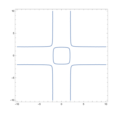
Figure 1. The space of real representations invariant under $\eta$, for $r=\tfrac{1}{10}$ ($\widetilde{r}=\tfrac{3}{10}$), which is the parabolic weight of our dodecahedron example.

3.7. Hitchin section

Consider a spin structure

$$S\longrightarrow T_{\tau}^{2}$$

on the rectangular torus $T_{\tau}^{2},$ i.e., $S^{\otimes 2}\cong K_{T^{2}_{\tau}}$, and the strictly stable and strongly parabolic Higgs bundle $(E,\widetilde{r},l_{0},\Phi)$ given by the data

$$E=S\oplus S;\quad r\in(0,\tfrac{1}{2});\quad l_{o}=\mathbb{C}S_{o}\oplus 0;\quad\Phi=\begin{pmatrix}0&0\\ dw&0\end{pmatrix}.$$

Then Hitchin-Kobayashi correspondence on non-compact curves [Si1] yields a compatible flat connection $\nabla$ satisfying

$$[\nabla]\in\mathcal{M}_{1,1}^{r}$$

with $\mathrm{SL}(2,\mathbb{R})$-monodromy. The underlying holomorphic bundle is hereby the non-trivial extension of $S$ by itself and the parabolic line $l_{0}$ is contained in the unique holomorphic line subbundle $S$ .

For every $q\in\mathbb{C}$ a strongly parabolic Higgs field

$$\Phi^{q}=\begin{pmatrix}0&qdw\\ dw&0\end{pmatrix}$$

on the parabolic bundle $(E,r,l_{o})$ corresponds to a compatible flat connection $\nabla^{q}$ with $[\nabla^{q}]\in\mathcal{M}_{1,1}^{r}$ having $\mathrm{SL}(2,\mathbb{R})$-monodromy (see Simpson [Si1]) – this is a particular instance of the so-called parabolic Hitchin-Kobayashi correspondence.

Lemma 3.19.

For fixed parabolic weight $r\in(0,\tfrac{1}{2})$, the element $[\nabla^{q}]\in\mathcal{M}_{1,1}^{r}$ is $\eta$-invariant if and only of $q\in\mathbb{R}.$

Proof.

The parabolic Higgs pairs $(E,r,l_{o},\Phi^{q})$ and $\eta^{*}\overline{(E,r,l_{o},\Phi^{q})}$ are gauge equivalent if and only if $q\in\mathbb{R}$. Therefore the Lemma follows from the Hitchin-Kobayashi correspondence for parabolic bundles. ∎

Lemma 3.20.

Let $\widetilde{r}=\frac{l}{k}\in(\frac{1}{4},\frac{1}{2})$ be rational with coprime $l,k\in\mathbb{N}$ and $r=2\widetilde{r}-\frac{1}{2}=\frac{4l-k}{2k}$. The connection $\nabla^{a,\chi,r}$ (on $T_{\tau}^{2}$) induces on $\Sigma_{g}$ as defined in (3.20) the trivial holomorphic structure if $\chi=\tfrac{\pi}{4\tau}\in\mathbb{R}$ modulo sign and lattice points. Likewise, the connection $\nabla^{a,\chi,r}$ (on $T_{\tau}^{2}$) induces on $\widetilde{\Sigma}_{g}$ (3.21) the trivial holomorphic structure if $\chi=i\tfrac{\pi}{4}\in\mathbb{R}$ modulo sign and lattice points.

Proof.

The proof is completely analogous to the proof of [BDHH, Proposition 3.1]. In fact it is just a reformulation of Lemma 3.16 using Lemma 3.14. ∎

In view of the above lemma we define

Definition 3.21.

We denote by $H\in$ Jac$(T^{2}_{\tau})$ the holomorphic structure (or the corresponding parabolic bundle on $\mathcal{S}_{4}$) that lifts to the trivial holomorphic structure over the associated compact Riemann surface $\Sigma$, i.e., either $H=\tfrac{\pi}{4\tau}$ for the sign choice $\sigma_{2}=1,\sigma_{3}=\sigma_{4}=-1$ and $\Sigma=\Sigma_{g},$ or $H=i\tfrac{\pi}{4}$ for $\sigma_{4}=1,\sigma_{2}=\sigma_{3}=-1$ and $\Sigma=\widetilde{\Sigma}_{g}.$

Remark 3.22.

If $H$ lies in the image of the map

$$q\in\mathbb{R}\longmapsto\chi(\nabla^{q})\in\text{Jac}(T^{2}_{\tau}),$$

the two Lemmas 3.19 and 3.20 show that the pull-back of the corresponding connection $\nabla^{q_{H}}$ to $\Sigma$ has trivial holomorphic structure and real monodromy representation.

4. Grafting and Spin Structures

4.1. Complex projective structures

Complex projective structures (or simply projective structures) on Riemann surfaces are classical objects in the theory of Riemann surfaces, see [Gu1] and the references therein. Consider an atlas $(U_{\alpha},z_{\alpha})_{\alpha\in\mathcal{U}}$ of a Riemann surface for which all the transition functions

$$z_{\beta}\circ z_{\alpha}^{-1}(z)=\frac{az+b}{cz+d}\quad\text{for some (constant)}\begin{pmatrix}a&b\\ c&d\end{pmatrix}\in\text{GL}(2,\mathbb{C})$$

are Möbius transformations. Such an atlas is called a (complex) projective atlas. Two projective atlases are equivalent if their union remains a projective atlas. An equivalence classes of projective atlases is a (complex) projective structure.

Naturally, the complex projective space $\mathbb{C}P^{1}$ itself is equipped with its standard projective structure. For elliptic curves the natural projective structure is obtained by identifying it with the flat torus $\mathbb{C}/\Lambda$. All transitions functions are in this case translations.

On a compact surface $\Sigma$ of genus $g\geq 2$ a special projective structure is provided by the uniformization theorem. In this case, there is a global biholomorphism from the universal cover of $\Sigma$ to Poincaré’s upper-half plane $\mathbb{H}^{2}\subset\mathbb{C}P^{1}$ which is equivariant with respect to a group homomorphism from the fundamental group of $\Sigma$ into the group of PSL$(2,\mathbb{R})$-valued Möbius transformations (with image a Fuchsian subgroup in PSL$(2,\mathbb{R})$). This map to the hyperbolic plane $\mathbb{H}^{2}\subset\mathbb{C}P^{1}$ coincides with the developing map of the unique hyperbolic metric (i.e. having constant curvature $-1$) on $\Sigma$ compatible with the complex structure.

In general, a complex projective structure on $\Sigma$ gives rise to a developing map $dev$ from the universal cover of $\Sigma$ to $\mathbb{C}P^{1}$ which is a local biholomorphism (but not necessarily a proper injective map). This developing map is equivariant with respect to a group homomorphism from the fundamental group of $\Sigma$ into PSL$(2,\mathbb{C})$ (uniquely defined up to conjugation in the Möbius group) which is referred to as the monodromy of the complex projective structure. By abuse of notation a complex projective structure is called a real projective structure if the corresponding monodromy takes values in PSL$(2,\mathbb{R})$ (up to conjugation in PSL$(2,\mathbb{C}))$ [Falt, Tak].

4.2. $\operatorname{SL}(2,\mathbb{C})$-Opers

A projective structure on a compact Riemann surface $\Sigma$ of genus $g\geq 2$ can also be described using particular flat $\operatorname{SL}(2,\mathbb{C})$-connections, called opers. Let $\nabla$ be a flat $\operatorname{SL}(2,\mathbb{C})$-connection on the rank two trivial smooth bundle $V=\underline{\mathbb{C}}^{2}\to\Sigma$ such that its induced holomorphic structure $\overline{\partial}^{\nabla}$ admits a holomorphic sub-line bundle $S$ of maximal degree $(g-1).$ Take a complementary $C^{\infty}$-bundle $S^{*}\subset V$ and write

$$\nabla=\begin{pmatrix}\nabla^{S}&\psi\\ \varphi&\nabla^{S^{*}}\end{pmatrix}$$ (4.1)

with respect to $V=S\oplus S^{*}.$ As $S$ is a holomorphic subbundle $\varphi$ is a $(1,0)$-form with values in Hom$(S,S^{*})$. Moreover, the flatness of $\nabla$ implies that

$$\varphi\in H^{0}(\Sigma,K_{\Sigma}(S^{*})^{2}).$$

If $\varphi\equiv 0$, then $S$ is a parallel sub-line bundle of $V$ with respect to the connection $\nabla$ and, consequently, it must have degree zero (and not $g-1$). Therefore, for $g\geq 2$ the holomorphic section $\varphi$ is not identically zero. Moreover, since the degree of $K_{\Sigma}(S^{*})^{2}$ is zero, the section $\varphi$ is nowhere vanishing. Therefore $S$ is a spin bundle, i.e., $S^{2}=K_{\Sigma}$ as holomorphic line bundles, and the section $\varphi$ can be identified with the constant section $\bf 1$ of the trivial holomorphic line bundle $\underline{\mathbb{C}}\rightarrow\Sigma$.

Definition 4.1.

A flat $\operatorname{SL}(2,\mathbb{C})$-connection of the form (4.1) on a compact Riemann surface is called an oper.

Given an oper $\nabla$ on the Riemann surfaces $\Sigma$ the induced projective structure is obtained as follows. Consider, on an open simply connected subset $U\subset\Sigma$, two linear independent $\nabla$-parallel sections of $V=S\oplus S^{*}$

$$\Psi_{1}=\begin{pmatrix}x_{1}\\ y_{1}\end{pmatrix},\quad\Psi_{2}=\begin{pmatrix}x_{2}\\ y_{2}\end{pmatrix}.$$

Then $y_{1}$ and $y_{2}$ are holomorphic sections of $S^{*}$ as the projection $V\to V/S$ is holomorphic. The quotient $z=y_{1}/y_{2}$ defines a holomorphic map to $\mathbb{C}P^{1}$. Choosing two other linear independent parallel sections

$$\widetilde{\Psi}_{1}=\begin{pmatrix}\widetilde{x}_{1}\\ \widetilde{y}_{1}\end{pmatrix}=a\Psi_{1}+b\Psi_{2}\quad\widetilde{\Psi}_{2}=\begin{pmatrix}\widetilde{x}_{2}\\ \widetilde{y}_{2}\end{pmatrix}=c\Psi_{1}+d\Psi_{2}$$

(with $ad-bc=1)$ amounts into

$$z=y_{1}/y_{2}\longmapsto\widetilde{z}=\widetilde{y}_{1}/\widetilde{y}_{2}=\frac{ay_{1}+by_{2}}{cy_{1}+dy_{2}}=\frac{az+b}{cz+d},$$

which is a Möbius transformation. Because $\varphi$ is nowhere vanishing, the map $z$ is unbranched, i.e., $z$ is a local (holomorphic) diffeomorphism, and we obtain a projective atlas.

4.3. Grafting

Grafting, or more precisely $2\pi$-grafting of the uniformization, introduced by Maskit [Mas], Hejhal [Hej] and Sullivan-Thurston [ST], is a procedure to obtain infinitely many distinct real projective structures. Our short description here follows Goldman [Go87].

Consider the real projective structure given by the uniformization (Fuchsian) representation of a Riemann surface $X$ and its developing map $dev$ to $\mathbb{H}^{2}\subset\mathbb{C}P^{1}$. Every non-trivial element of the first fundamental group $[\gamma]\in\pi_{1}(X)$ can be represented by a unique geodesic $\gamma\subset X$ with respect to the constant curvature $-1$ metric on $X$ (up to orientation). Under the developing map $\gamma$ is mapped to a circular arc. The corresponding full circle $C$ intersects the boundary at infinity of the hyperbolic disc at two points. The monodromy of the uniformization representation along $\gamma$ is given by an element $A\in\operatorname{SL}(2,\mathbb{R})$, unique up to sign. The sign depends on the lift of the monodromy representation from ${\rm PSL}(2,\mathbb{R})$ to $\operatorname{SL}(2,\mathbb{R})$.

On the other hand, a hyperbolic transformation conjugated to $A\in\operatorname{SL}(2,\mathbb{R})$ gives rise to a Hopf torus $T_{A}$ endowed with a projective structure as follows. There exist two (unique) circles $S_{1}$ and $S_{2}\subset\mathbb{C}P^{1}$ that are invariant under the transformation $A.$ Let $C_{1}$ be another circle in $\mathbb{C}P^{1}$ intersecting both $S_{1}$ and $S_{2}$ perpendicularly, and consider $C_{2}=A(C_{1}).$ Since $C_{1}$ and $C_{2}$ have no intersection points, they bound an annulus $\mathbb{A}$. The torus $T_{A}$ is then obtained from gluing $C_{1}$ and $C_{2}$ via $A$ and possesses by construction a projective structure. The monodromy of the corresponding projective structure on $T_{A}$ is trivial along $C_{1}$, while it is $A$ along the curve obtained from projecting the arc on $S_{1}$ between the intersection points with $C_{1}$ and $C_{2}=A(C_{1})$. When cutting $T_{A}$ along $S_{1}$ (rather than $C_{1}$) we obtain another annulus and we denote this cylinder together with its two boundary components by $|T_{A}|.$

Grafting along the geodesic $\gamma\subset X$ glues $X$ and the appropriate Hopf torus $T_{A}$ for the hyperbolic $A\in\operatorname{SL}(2,\mathbb{R})$ representing the monodromy along $\gamma$. More explicitly, let $S_{1}$ be the unique circle in $\mathbb{C}P^{1}$ containing the image of the geodesic $\gamma$ under the uniformization map, and $S_{2}$ be the boundary of $\mathbb{H}^{2}.$ Then each of the two boundary components of $|T_{A}|$ can be identified with the image of the geodesic $\gamma.$ Therefore, $X\setminus\gamma$ and $|T_{A}|$ can be glued to obtain a new Riemann surface $X^{G}$ without boundary (the notation $X^{G}$ stands for grafted $X$). Moreover, the induced new projective structure has the same monodromy as the uniformization of $X$. In particular, it is a real projective structure. Note that (the developing map $dev_{G}$ of) the projective structure on $X^{G}$ induces a curvature -1 metric away from a singularity set. The singularity set is given by the intersection of the annulus $\mathbb{A}$ with the circle $S_{2}$ considered as the boundary of the hyperbolic plane $\mathbb{H}^{2}$ consisting of two smooth curves that are both, considered as curves in $X^{G}$, closed and homotopic to $\gamma$.

Iteration leads to the construction of infinitely many Riemann surfaces with distinct real projective structures, but their monodromy remains the same uniformization monodromy of the initial Riemann surface $X$. Altogether, starting with the isotopy class $\mathcal{C}$ of a simple closed curve on $X$, and applying the grafting construction along the closed curve yields (infinitely many) different Riemann surfaces of the same genus with real projective structures. We will refer to grafting along a simply closed geodesic $\gamma$ once as simple-grafting and neglect the possibility of grafting multiple times along the same geodesic in the following.

Remark 4.2.

In what follows, $\Sigma$ will be the Riemann surface $X^{G}$ obtained from grafting (once) the Riemann surface $\Sigma^{uG}:=X$, where the superscript ${uG}$ stands for ungrafting.

4.4. Spin structures

Let $\Sigma$ be a compact Riemann surface of genus $g$. A spin structure is a choice of a holomorphic line bundle $S$ with

$$S^{\otimes 2}=K_{\Sigma}.$$

Two spin bundles differ by a holomorphic line bundle which squares to the trivial holomorphic line bundle. If we equip this holomorphic line bundle with its unique flat unitary connection, its monodromy takes values in $\mathbb{Z}_{2}$ (as the monodromy squares to the identity). Such a holomorphic line bundle together with its flat connection is called a $\mathbb{Z}_{2}$-bundle. It is determined by its monodromy representation which is a group homomorphism from the fundamental group of $\Sigma$ into the abelian group $\mathbb{Z}_{2}.$ Hence the space of spin structures is an affine space with underlying translation vector space $H_{1}(\Sigma,\mathbb{Z}_{2})$.

From a topological point of view, a spin structure is given by a quadratic form

$$Q\colon H_{1}(\Sigma,\mathbb{Z}_{2})\to\mathbb{Z}_{2},$$

whose underlying bilinear form is the intersection form (mod 2), see [John, At]. The relationship between these two viewpoints can be explained as follows: Fix a given line bundle $S$ with $S^{\otimes 2}=K_{\Sigma}.$ Then, for every closed and immersed curve $\delta\colon S^{1}\to\Sigma$ there is a unique $\omega\in\Gamma(S^{1},\delta^{*}K_{\Sigma})$ with

$$\omega(\delta^{\prime})=1.$$

Let $\widetilde{\delta}\,\colon\,\mathbb{R}\,\longrightarrow\,\Sigma$ be the immersed curve defined as the lift of $\delta$ to the universal covering $\mathbb{R}\to S^{1}$. Consider the pull-back $\widetilde{\omega}$ of $\omega$ to a (non-vanishing) section of $\widetilde{\delta}^{*}K_{\Sigma}$. Up to sign, there exists a unique section

$$\widetilde{s}\,\in\,\Gamma(\mathbb{R},\,\widetilde{\delta}^{*}S)$$

such that $\widetilde{s}^{2}\,=\,\widetilde{\omega}$. The $\mathbb{Z}_{2}$-monodromy of $S$ along $\delta$ is $1$ if $\widetilde{s}$ (or, equivalently, $-\widetilde{s}$) is invariant by the action of the fundamental group of $S^{1}$ on $\mathbb{R}$ by deck-transformations. The $\mathbb{Z}_{2}$-monodromy of $S$ along $\delta$ is $-1$ if $\widetilde{s}$ is transformed in $-\widetilde{s}$ by the action of the generator of the fundamental group of $S^{1}$ on $\mathbb{R}$. This $\mathbb{Z}_{2}$-monodromy only depends on the class of $\delta$ in $H_{1}(\Sigma,\mathbb{Z}_{2})$. Associating to the class of $\delta$ in $H_{1}(\Sigma,\mathbb{Z}_{2})$ the above monodromy with values in $\mathbb{Z}_{2}$ uniquely determines a quadratic form $Q\colon H_{1}(\Sigma,\mathbb{Z}_{2})\to\mathbb{Z}_{2}$ whose underlying bilinear form is the intersection form (mod 2), and hence a topological spin structure, see [John] and also [P] and [Bob, Section 10].

4.4.1. Spin structures and opers

Let $\nabla$ be an oper on $V\to\Sigma$ given by (4.1) corresponding to real projective structure, i.e., its monodromy takes values in

$$P\mathrm{SL}(2,\mathbb{R})=\text{Isom}(\mathbb{H}^{2}).$$

The isomorphism between $S^{\otimes 2}$ and $K_{\Sigma}$ can be made explicit in two equivalent ways.

First, consider for $p\in\Sigma$ an arbitrary $s_{p}\in S_{p}\subset V_{p},$ then

$$\nabla s_{p}\wedge s_{p}\in(K_{\Sigma})_{p}$$

is well-defined and gives rise to a bilinear map $S_{p}\times S_{p}\to(K_{\Sigma})_{p},$ since $S$ is a holomorphic subbundle of $V.$ This bilinear form is non-degenerate, as $\varphi$ is non-vanishing, and defines a holomorphic isomorphism between $S^{\otimes 2}$ and $K_{\Sigma}.$ Likewise, consider the (locally defined) parallel sections

$$\Psi_{1}=\begin{pmatrix}x_{1}\\ y_{1}\end{pmatrix},\Psi_{2}=\begin{pmatrix}x_{2}\\ y_{2}\end{pmatrix}\in\Gamma(U,S\oplus S^{*}).$$

determined by the initial condition

$$(\Psi_{1})_{p}=\begin{pmatrix}s_{p}\\ 0\end{pmatrix}\quad\text{and}\quad(\Psi_{2})_{p}=\begin{pmatrix}0\\ t_{p}\end{pmatrix}$$

with

$$(t_{p},s_{p})=1.$$

Then, a direct computation shows

$$s_{p}\otimes s_{p}=\omega_{p}\in(K_{\Sigma})_{p}$$

where

$$\omega\,=\,-d(\tfrac{y_{1}}{y_{2}}).$$

Another way to obtain the spin bundle $S$ is the following. The standard projective structure on $\mathbb{C}P^{1}$ is induced by the trivial connection $d$ on the trivial holomorphic rank 2 bundle. Its spin bundle is the tautological bundle $\mathcal{O}(-1),$ i.e, the fiber at $l\in\mathbb{C}P^{1}$ is the line $l.$ Consider for a general Riemann surface $\Sigma$ a projective structure and developing map $dev$ induced by an oper $(V,\nabla)$. Let $M$ be the monodromy homomorphism of $\nabla$. Then the bundle $V$ is given by the twisted bundle

$$V\,=\,(\widetilde{\Sigma}\times\mathbb{C}^{2})/\sim,$$

where $(p,v)\sim(\widetilde{p},\widetilde{v})$ if and only if $\widetilde{p}=\gamma_{*}p$ and $\widetilde{v}=M_{\gamma}v$ for a $\gamma\in\pi_{1}(\Sigma).$ The spin bundle $S$ is then given by the twisted pull-back of the tautological bundle $\mathcal{O}(-1)\rightarrow\mathbb{C}P^{1}$ via the developing map

$$S=dev^{*}\mathcal{O}(-1)/\sim.$$ (4.2)

Due to its topological invariance, continuous deformations of the Riemann surface and the oper do not change the (topological) spin structure. (For closed curves in the moduli space of Riemann surfaces that are not null-homotopic, the deformation of the spin structure along the curve might have monodromy, see for example [At]. This corresponds to a non-trivial action of the mapping class group.)

Note that the difference between two quadratic forms on $H_{1}(\Sigma,\mathbb{Z}_{2})$ corresponding to spin structures is given by a linear form on $H_{1}(\Sigma,\mathbb{Z}_{2})$, see [John].

Lemma 4.3.

Let $\Sigma$ be a compact Riemann surface. The uniformization connection $\nabla^{U}$ and the simple-grafting connection $\nabla^{G}$, along an isotopy class $\mathcal{C}$ of a simple non-null-homotopic curve $\mathcal{C}$ on $\Sigma$, (whose monodromy lies in the same connected component of real representations) induce different spin structures on the Riemann surface $\Sigma.$ More precisely, the difference of the corresponding spin structures is determined by the linear form on $H_{1}(\Sigma,\mathbb{Z}_{2})$ obtained by inserting a representative of the class $\mathcal{C}\in H_{1}(\Sigma,\mathbb{Z}_{2})$ into the intersection form mod 2 on $\Sigma$.

Remark 4.4.

Clearly, the lemma generalizes to multiple graftings as well.

Proof.

Consider the Riemann surface $\Sigma^{uG}=X$ (obtained by ungrafting), i.e., its uniformization connection is gauge equivalent to $\nabla^{G}$. Since the two complex structures on $\Sigma^{uG}$ and $\Sigma,$ viewed as two points in the Teichmüller space of genus $g$ surfaces, can be connected by a smooth curve, both uniformization connections (in the same connected component of real points in the de Rham moduli space) on $\Sigma^{uG}$ and $\Sigma$ induce the same topological spin structure. It remains to show that grafting once (from the uniformization oper of $\Sigma^{uG}$ to the oper $\nabla^{G}$ on $\Sigma$) changes this spin structure.

Recall that we can compute the value of the quadratic form $Q$ associated to the spin structure on the class in $H^{1}(\Sigma,\mathbb{Z}_{2})$ of an immersed curve $\delta\colon S^{1}\to\Sigma$ by considering the lifting $\widetilde{\omega}\,\in\,\Gamma(\mathbb{R},\,\widetilde{\delta}^{*}K_{\Sigma})$ to the universal cover of $S^{1}$ of the unique section $\omega\in\Gamma(S^{1},\delta^{*}K_{\Sigma})$ defined by $\omega(\delta^{\prime})=1$ and then considering the $\mathbb{Z}_{2}$-monodromy defined by a section $\widetilde{s}\,\in\,\Gamma(\mathbb{R},\,\widetilde{\delta}^{*}S)$ such that $\widetilde{s}^{2}\,=\,\widetilde{\omega}$.

Along closed curves representing an element of $\pi_{1}(\Sigma)$ that do not intersect the (simple) grafting curve $\gamma$, the developing map does not change. Therefore, by (4.2) the quadratic form of the spin structure specialized on those curves remains the same.

Consider the closed curve $\delta_{1}$ in $\Sigma^{uG}$ which intersects the grafting curve $\gamma$ once. The developing map along the corresponding closed curve $\delta$ on $\Sigma$ (which intersects the grafting curve $\gamma$ once) is obtained from the developing map along $\delta_{1}$ by precomposing it with the circle $C_{1}$ along the Hopf cylinder $T_{A}$ . With respect to the holomorphic 1-form $dz$ on $\mathbb{C}P^{1}\setminus\{\infty\}$ and for $C_{1}=\{ae^{i\theta}+b\;|\;\theta\in[0,2\pi]\}$ for appropriate $a>0,b\in\mathbb{C}$, the section $\omega$ of the canonical bundle, along $C_{1}$, is given by

$$\omega_{\mid\theta}=-ia^{-1}e^{-i\theta}dz.$$

Using (4.2) we can use the holomorphic section $\sqrt{dz}=(z,1)$ on $\mathbb{C}P^{1}\setminus\{\infty\}$ along $C_{1}$ and observe that a section $s$ of $S$, along $C_{1}$, such that $s^{2}=\omega$ is given by

$$s(\theta)=\sqrt{-ia^{-1}}e^{-\tfrac{i\theta}{2}}\sqrt{dz}.$$

Hence, specialized on the closed curve $\delta$, the quadratic form associated to the spin structure of the oper $\nabla^{G}$ on $\Sigma$ differs from the quadratic form of the spin structure induced by the uniformization oper of $\Sigma^{G}$ by a $-1$ factor. This completes the proof. ∎

4.5. Grafting on the 1-punctured torus $T^{2}_{\tau}$

Fix the parabolic weight $r\in(0,\frac{1}{2})$ and consider the real subspace $\mathcal{M}_{1,1}^{r}(\mathbb{R})$ of $\mathcal{M}_{1,1}^{r}$ corresponding to the real character variety. By [Go03, Theorem 3.4.1] each non-compact connected component of the real character variety $\mathcal{M}_{1,1}^{r}(\mathbb{R})$ is in one-to-one correspondence to hyperbolic structures on the one-punctured torus with conical angle $4\pi r$ at the marked point (as the rotation angle satisfies $\theta=2r$). Therefore, we refer to elements of $\mathcal{M}_{1,1}^{r}(\mathbb{R})$ as conical hyperbolic structures for short. For conical hyperbolic structures [Bu, Theorem 1.5.2] shows that every free homotopy class of curves on the torus can be represented by a simply closed geodesic.

Fix a real representation $\rho\in\mathcal{M}_{1,1}^{r}(\mathbb{R})$ and denote by $X,\,Y\in\operatorname{SL}(2,\mathbb{R})$ its values along $\gamma_{x},\,\gamma_{y}\,\in\,\pi_{1}(T^{2}_{\tau}\setminus\{0\},\,p_{0}),$ respectively (see (3.5) and (3.6)). Then the corresponding conical hyperbolic structure constructed in [Go03, Theorem 3.4.1] is obtained by gluing the opposite edges of a particular hyperbolic quadrilateral $P_{1}P_{2}P_{3}P_{4}.$ The point $P_{4}$ hereby is a fixed point in the hyperbolic plane $\mathbb{H}^{2}$ with (elliptic) local monodromy given by $r$, while

$$P_{3}=X\cdot P_{4},\quad P_{2}\,=\,Y\cdot X\cdot P_{4}\quad\text{ and }\quad P_{1}\,=\,X^{-1}\cdot Y\cdot X\cdot P_{4}.$$

Consider now in the hyperbolic plane $\mathbb{H}^{2}$ the unique hyperbolic geodesic $c$ perpendicular to both geodesics generated by $P_{1}P_{2}$ and $P_{4}P_{3}$. Due to its uniqueness, this geodesic is fixed by $Y$ (it is the axis of the loxodromic isometry $Y$). Moreover, since two distinct geodesics in $\mathbb{H}^{2}$ intersect at most once, $c$ does not contain any of the vertices $P_{j}$, for all $j=1,\,...,\,4$. Hence $c$ is a simply closed geodesic representing the free homotopy class of $\gamma_{y}$ and $c$ does not contain the conical point. The same argument shows the existence of a unique hyperbolic geodesic $\widetilde{c}$ perpendicular to both geodesics generated by $P_{1}P_{4}$ and $P_{2}P_{3}$ representing the free homotopy class of $\gamma_{x}$ that does not contain the conical point.

Therefore, grafting of conical hyperbolic structures can be performed along both geodesics representing the free homotopy class of $\gamma_{x}$ and $\gamma_{y}$.

Lemma 4.5.

The conical hyperbolic structure on the torus is rectangular if and only if

$$\operatorname{tr}(YX)=\operatorname{tr}(YX^{-1}).$$

Proof.

The trace condition $\operatorname{tr}(YX)=\operatorname{tr}(YX^{-1})$ implies that the reflexion across the unique geodesic $c$, which sends the edge $P_{2}P_{3}$ to the edge $P_{1}P_{4},$ induces a real symmetry of the conical hyperbolic structure. The fix point set consists of two disjoint circles – the geodesic $c$ and the edge $P_{2}P_{3}$ (which is identified with the edge $P_{1}P_{4}$). Hence the corresponding torus is rectangular (and not rhombic) and the reflexion across $c$ coincides with the reflexion across the edge $P_{1}P_{4}$ (this reflexion corresponds to the involution $i\eta$ described in Section 3.4). ∎

Orbifold grafting is well-defined on the one-punctured torus and the grafted Riemann surface remains rectangular:

Lemma 4.6.

Grafting the $1$-punctured rectangular torus $T^{2}_{\tau}=\mathbb{C}/\Gamma$, $\Gamma=\mathbb{Z}\oplus i\tau\mathbb{Z},$ along $\gamma_{x}$ or $\gamma_{y}$, respectively, yields another $1$-punctured and rectangular torus $T^{2}_{\tau^{G}}$ with a different real projective structure.

Proof.

Let $Y\in\operatorname{SL}(2,\mathbb{R})$ denotes the monodromy along $\gamma_{y}$. Since $y=\operatorname{tr}(Y)$ satisfies $|y|>2$, we get that $Y$ is a hyperbolic element in $\operatorname{SL}(2,\mathbb{R}).$ Therefore, grafting glues the annulus $|T_{Y}|$ to $T^{2}_{\tau}$ along $\gamma_{y}$. This adds a rectangle to the fundamental domain of the torus $T^{2}_{\tau}$ along the edge $\gamma_{y}$. Therefore, the resulting torus remains rectangular and $\tau$ decreases. With the same argument grafting along $\gamma_{x}$ add a rectangle along the edge $\gamma_{y}$ and the conformal type of $\tau$ increases. ∎

On the grafted punctured torus we fix (without loss of generality) the real involution, which we again denote by $\eta,$ whose fix point set lies in the homology class $2[\gamma_{x}]$ and contains the singular point. Let

$$\mathcal{M}_{\mathbb{R}}^{r}=\mathcal{M}_{1,1}^{r,\eta}\cap\mathcal{M}_{1,1}^{r}(\mathbb{R})\subset\mathcal{M}_{1,1}^{r}$$

be the subset of $\eta$-symmetric $\text{SL}(2,\mathbb{R})$-representations on the one-punctured torus with local monodromy determined by the parabolic weight $r$. From (3.8) and Lemma 3.17 (see also Remark 3.18 and Figure 1) the space $\mathcal{M}_{\mathbb{R}}^{r}$ has four connected components, each of them is a non-compact manifold of real dimension one.

Lemma 4.7.

Let $\rho\in\mathcal{M}_{\mathbb{R}}^{r}$. Then there is a unique $\tau\in\mathbb{R}^{>0}$ such that the uniformization representation $\rho^{U}(\tau)$ of the 1-punctured torus $T^{2}_{\tau}$ satisfies $\rho=\rho^{U}(\tau)$.

Proof.

The proof of [Go03, Theorem 3.4.1] which identifies each connected component of $\mathcal{M}_{1,1}^{r}(\mathbb{R})$ with conical hyperbolic structures also implies that the one-dimensional submanifold of $\eta$-symmetric representations $\mathcal{M}_{\mathbb{R}}^{r}$ is given by those hyperbolic structures compatible with the rectangular conformal structure of $T^{2}_{\tau}$, i.e., $\tau\in\mathbb{R}^{>0}$. ∎

The following Lemma is analogous to the main result of [Tan].

Lemma 4.8.

For each $r\in(0,\tfrac{1}{2})$, simple-grafting (along $\gamma_{x}$ or $\gamma_{y}$) induces a homeomorphism of the Teichmüller space $\mathbb{R}_{>0}$ of 1-punctured rectangular tori to itself.

Proof.

Without loss of generality we only consider grafting along $\gamma_{y}.$ The map $\tau\mapsto\tau^{G}$, see Lemma 4.6, is smooth and moreover, $\tau^{G}\,<\,\tau$. Therefore, $\tau^{G}\rightarrow 0$ for $\tau\rightarrow 0.$ For surjectivity we use the intermediate value theorem: it remains to show $\tau^{G}\rightarrow\infty$ for $\tau\rightarrow\infty$. This follows by observing that the conformal type $\tau_{Y}$ of the Hopf torus $T_{Y}$ satisfies $\tau_{Y}\to\infty$ when $\tau\to\infty$ and $\tau^{G}=(\tfrac{1}{\tau}+\tfrac{1}{\tau_{Y}})^{-1}$. Injectivity follows from the fact that the conformal type of the Hopf tori $T_{Y}$ and $T_{\widetilde{Y}}$ satisfies $\tau_{Y}>\tau_{\widetilde{Y}}$ for $\tau>\widetilde{\tau}$. ∎

4.6. Spin structures and projective structures on the 1-punctured torus

If the underlying holomorphic line bundle $L$ of a logarithmic SL$(2,\mathbb{C})$-connection on the 1-punctured torus in (3.12) is not a spin bundle, then the corresponding $\gamma_{\chi}^{\pm}$ must have a zero. Thus an oper $\nabla$ on a 1-punctured torus gives rise to a spin bundle on the compact torus through the special form of the connection in (3.14) and (3.15).

Moreover, the corresponding quadratic form (see Section 4.4) $Q$ on $H_{1}(T^{2}_{\tau}\setminus\{o\},\,\mathbb{Z}_{2})$ is well defined on $H_{1}(T^{2}_{\tau},\,\mathbb{Z}_{2})$, as the local conjugacy class around the puncture is trivial in $\mathbb{Z}_{2}$, see also [John, Bob]. Hence, using the same arguments as in the compact case, an suitably adjusted version of Lemma 4.3 holds on the one-punctured torus, i.e., grafting changes the induced spin structure.

The grafted connection $\nabla^{G}$ has by construction SL$(2,\mathbb{R})$-monodromy lying in the same connected component as the orbifold uniformization connection $\nabla^{U}$ of $T^{2}_{\tau}.$ Moreover, the Hitchin section based at $T^{2}_{\tau}$ maps $q=0$ to $\nabla^{U}$ and there exist a $q_{G}\in\mathbb{R}_{*}$ with $\nabla^{q_{G}}=\nabla^{G}$ by $\eta$-invariance.

Recall that we have chosen the spin structure of $\nabla^{U}$ to be trivial, i.e., it is represented by $\chi(\nabla^{U})=0\in$ Jac$(T^{2}_{\tau}).$ For the grafted connection $\nabla^{G}$ it turns out, using abelianization, that the underlying line bundle $L$ must be a particular spin bundle, i.e., $\chi(\nabla^{G})$ is a half lattice point of Jac$(T^{2}_{\tau})$.

Lemma 4.9.

Via abelianization the spin structure of simple-grafting along $\gamma_{y}$ is given by $\chi(\nabla^{G,y})=i\tfrac{\pi}{2}$ (up to lattice points and sign), and the spin structure of simple-grafting along $\gamma_{x}$ is given by $\chi(\nabla^{G,x})=\tfrac{\pi}{2\tau}$ (up to lattice points and sign),

Proof.

The unitary line bundle connection on the induced spin bundle for $\chi(\nabla^{G,y})$ is

$$d+i\tfrac{\pi}{2}d\overline{w}+i\tfrac{\pi}{2}dw$$

which has monodromy $-1$ along $\gamma_{x}$ and monodromy $1$ along $\gamma_{y}$. For $\chi(\nabla^{G,x})$ it is

$$d+\tfrac{\pi}{2\tau}d\overline{w}-\tfrac{\pi}{2\tau}dw$$

and has monodromy $-1$ along $\gamma_{y}$ and monodromy $1$ along $\gamma_{x}$. Thus, the statement follows by the same arguments as Lemma 4.3, since after grafting along $\gamma_{y}$ the spin structure change by multiplication with $1$ along $\gamma_{y}$ (meaning unchanged) and by multiplication with $-1$ along $\gamma_{x}$. It is the other way around when grafting along $\gamma_{x}.$ ∎

5. Holomorphic connections with $\operatorname{SL}(2,\mathbb{R})$-monodromy

Consider the natural 2-fold covering map $\pi\colon Jac(T^{2}_{\tau})\to\mathbb{C}P^{1}$ branched at the four spin bundles. The real subspace provided by Lemma 3.10 is mapped to $\mathbb{R}\subset\mathbb{C}$. In fact, as the corresponding elliptic curve $T^{2}_{\tau}$ being rectangular, its associated $\wp$-function maps the four spin bundles in the Jacobian (which identifies with the half periods and the critical points of $\wp$) to the real axis.

Lemma 5.1.

The map $h\colon\mathbb{R}\rightarrow\mathbb{R}\subset\mathbb{C}P^{1}=\pi(\text{Jac}(T^{2}_{\tau}))$ given by $q\mapsto\pi(\chi(\nabla^{q}))$ is continuous. Moreover, there exists $q_{H}\in\mathbb{R}\setminus\{0\}$ satisfying either $\chi(\nabla^{q_{H}})=\frac{\pi}{4\tau}$ or $\chi(\nabla^{q_{H}})=i\frac{\pi}{4}$ (up to sign and adding lattice points).

Proof.

The holomorphic structure $\chi(\nabla^{q})$ as a map into Jac$(T^{2}_{\tau})$ is only well-defined up to sign. The projection to $\mathbb{C}P^{1}$ removes this multivaluedness, and $h$ is well-defined and continuous. It should be noted that this is, up to normalisation, the Tu-invariant of $\nabla^{q}$ in [Lo]. By $\eta$-invariance, i.e., Lemma 3.19 and Lemma 3.10, and using the fact that $\pi$ maps exactly the (real) $\eta$-invariant points of the Jacobian (i.e., $\chi$ lying in the lines given by Lemma 3.10) to real points (including $z=\infty$) in $\mathbb{C}P^{1}$, we obtain that $h\colon\mathbb{R}\to\mathbb{R}P^{1}\subset\mathbb{C}P^{1}.$

Grafting along $\gamma_{y}$ (or $\gamma_{x}$) changes the spin structure by Lemma 4.9. The map $h$ sends the point $q=0$ to $0\in$ Jac$(T_{\tau}^{2})$ and the point $q=q_{G}$ to $i\tfrac{\pi}{2}\in$Jac$(T_{\tau}^{2})$ (or to $\tfrac{\pi}{2\tau}\in$Jac$(T_{\tau}^{2})$).

By continuity the image of $h$ contains either the interval $\pi([0,i\frac{\pi}{2}])\subset\mathbb{R}P^{1},$ where

$$[0,i\tfrac{\pi}{2}]:=\{ti\tfrac{\pi}{2}\mid 0\leq t\leq 1\}$$

and analogously for the subsequent intervals, or the closure of its complement (inside $\mathbb{R}P^{1}$) given by

$$\mathbb{R}P^{1}\setminus\pi((0,i\tfrac{\pi}{2}))=\pi([0,\tfrac{\pi}{2\tau}])\cup\pi([\tfrac{\pi}{2\tau},\tfrac{\pi}{2\tau}+i\tfrac{\pi}{2}])\cup\pi([\tfrac{\pi}{2\tau}+i\tfrac{\pi}{2},i]).$$

Consequently, there exists $q_{H}$ (and a second $\widetilde{q}_{H}$ for grafting along $\gamma_{x}$) in the interval between $q=0$ and $q=q_{G}$ such that $\chi(\nabla^{q_{H}})=\frac{\pi}{4\tau}$ or $\chi(\nabla^{q_{H}})=i\frac{\pi}{4}$ (up to sign and adding lattice points). ∎

Remark 5.2.

The Lemma shows that the holomorphic structure $H$ (see Definition 3.21) which lifts to the trivial holomorphic structure on the associated Riemann surface $\Sigma$ is attained whenever the weight $r$ is rational. Since the map $h$ depends continuously in $\tau$, the bundle type $H$ does not change for a continuous deformation of $\tau.$

Lemma 3.20 together with Remark 3.22 gives the following theorem.

Theorem 5.3.

For every rational weight $\widetilde{r}=\tfrac{l}{k}\in(\frac{1}{4},\frac{1}{2})$ and every $\tau\in\mathbb{R}_{>0}$, the Riemann surface $\Sigma(\tau)$ given by the $g+1$-fold covering (3.20) or (3.21) (with $g=k-1$ for k odd and $g=k/2-1$ for $k$ even) of the four punctured sphere $\mathcal{S}_{4}(\tau)$ (as in (3.10)) admits a holomorphic connection on the trivial bundle $\underline{\mathbb{C}}^{2}\rightarrow\Sigma(\tau)$ with SL$(2,\mathbb{R})$-monodromy.

Remark 5.4.

Restricting to rational weights $r=\tfrac{k-1}{2k}$ we obtain a new proof of the main theorem of [BDHH], without applying the WKB analysis. In particular, we obtain holomorphic systems on compact Riemann surfaces with Fuchsian representations that are not far out in the Betti moduli space of real representations.

Corollary 5.5.

The triple $\nabla^{U},$ $\nabla^{H}$ and $\nabla^{G}$ is ordered in the character variety, i.e., either

$$y(\nabla^{U})<y(\nabla^{H})<y(\nabla^{G})\quad\text{ or }\quad y(\nabla^{U})>y(\nabla^{H})>y(\nabla^{G}).$$

Proof.

From (3.22), each connected component of $\mathcal{M}_{\mathbb{R}}^{r}$ admits $y=\operatorname{tr}(Y)$ as a global coordinate, where $Y$ is defined as the monodromy along $\gamma_{y}$ (see (3.6)). Moreover, the image of $y$ is either $(2,\infty)$ or $(-\infty,-2).$

Hence, for any choice of spin structure on the torus the map

$$q\in\mathbb{R}\rightarrow y(\nabla^{q})\in\mathbb{R}$$

is a diffeomorphism onto the corresponding connected component given by $y\in(2,\infty)$ or $y\in(-\infty,-2).$ Therefore, the map $y(\nabla^{q})$ is strictly monotonic in $q\in\mathbb{R}$ and the Corollary follows from $q_{H}$ lying between $q=0$ and $q=q_{G}.$ ∎

Remark 5.6.

With the above notations, since $q\in\mathbb{R}$ (by Hitchin-Kobayashi correspondence) and $y\in(2,\infty)$ (the trace) are both global coordinates on every connected component of $\mathcal{M}^{r}_{\mathbb{R}},$ the space of $\eta$-invariant conical hyperbolic structures, we have that $y(\nabla^{q})$ is either strictly monotonically increasing or decreasing. Moreover, the conformal type for grafting $n$-times along $\gamma_{x}$ and $n$-times along $\gamma_{y}$ degenerate for $n\rightarrow\infty$ to the two different ends of $\mathcal{M}^{r}_{\mathbb{R}}$. Therefore, either

$$y(\nabla^{q_{G,x}})<y(\nabla^{q=0})<y(\nabla^{q_{G,y}})\quad\text{ or }\quad y(\nabla^{q_{G,x}})>y(\nabla^{q=0})>y(\nabla^{q_{G,y}}).$$

Since the $y$-coordinate of connection $\nabla^{q_{H}}$ lies between $y(\nabla^{q_{G,x}})$ and $y(\nabla^{q=0})$, or respectively, $y(\nabla^{q_{H}})$ lies between $y(\nabla^{q_{G,y}})$ and $y(\nabla^{q=0})$, we reverse the ordering in Corollary 5.5 by grafting along $\gamma_{x}$ instead of $\gamma_{y}$.

Lemma 5.7.

Consider the family of 1-punctured rectangular tori $T^{2}_{\tau}$, for $\tau\in\mathbb{R}_{>0}$. Then the map defined using the abelianization coordinates

$$\mathfrak{M}\colon\mathbb{R}^{2}\ni(a,\tau)\rightarrow\mathcal{M}_{1,1}^{r,\eta},\quad(a,\tau)\mapsto\rho(\nabla^{a,\chi_{0}}(\tau))$$

is a local diffeomorphism for fixed $\chi_{0}=\tfrac{\pi}{4\tau}$ away from $a_{0}=-\tfrac{\pi}{4\tau}.$

Remark 5.8.

An analogue Lemma also holds when choosing $\chi_{0}=i\tfrac{\pi}{4}$ and $a\in i\mathbb{R}$ away from $a_{0}=i\tfrac{\pi}{4}.$

Proof.

Consider the map

$$\widetilde{\mathfrak{M}_{\mathbb{C}}}\colon\mathbb{C}^{3}\ni(a,\chi,\tau)\rightarrow\mathcal{M}_{1,1}^{r},\quad(a,\chi,\tau)\mapsto\rho(\nabla^{a,\chi}(\tau))$$

from $\mathbb{C}^{3}$ to the complex 2-dimensional space $\mathcal{M}^{r}_{1,1}.$ By the Riemann-Hilbert correspondence and the fact that, for fixed conformal type $\tau$, the variables $(a,\chi)$ are coordinates of $\mathcal{M}_{1,1}^{r}$ (away from half lattice points of $\chi$), the kernel of the differential is only $1$-dimensional, and can be computed using the differential of isomonodromic deformations.

To show that $\mathfrak{M}$ is a local diffeomorphism, it suffices to prove that

$$\mathfrak{M}_{\mathbb{C}}\colon\mathbb{C}^{2}\ni(a,\tau)\rightarrow\mathcal{M}_{1,1}^{r},\quad(a,\tau)\mapsto\rho(\nabla^{a,\chi_{0}}(\tau))$$

is an immersion at all points $(a,\tau)\in\mathbb{C}^{2}$, with $a\neq-\tfrac{\pi}{4\tau}$ (i.e., without restricting to the $\eta$-invariant subspaces). Indeed, Lemma 3.10 then implies that the image of $\mathfrak{M}_{\mathbb{C}}$ restricted to real points $(a,\tau)\in\mathbb{R}^{2}$ lies in the real 2-dimensional submanifold $\mathcal{M}_{1,1}^{r,\eta}\subset M_{1,1}^{r}$.

Since $\mathfrak{M}_{\mathbb{C}}$ is obtained from $\widetilde{\mathfrak{M}_{\mathbb{C}}}$ by fixing the $\chi$-coordinate, it suffices to show the kernel of $d\widetilde{\mathfrak{M}_{\mathbb{C}}}$ is transversal to the slice $\chi=\chi_{0}.$ The proof uses a result by Loray [Lo]. Be aware that the parameter $\tau$ used here is the conformal type of the torus $T^{2}_{\tau},$ while the parameter $t\in\mathbb{C}P^{1}$ in [Lo] is the conformal type of the $4$-punctured sphere with punctures $\{0,1,\infty,t\}$. The transformation from $\tau$ to $t\in\mathbb{C}P^{1}$ is a local diffeomorphism since the conformal type of the torus is non-degenerated.

First note that, for every fixed $\tau$, the parameters $\chi_{0}(\tau)=\tfrac{\pi}{4\tau}$ and $a_{0}(\tau)=-\tfrac{\pi}{4\tau}$ define a reducible connection on the 4-punctured torus $\Sigma_{2}(\tau)=\mathbb{C}/(2\mathbb{Z}\oplus 2\tau i\mathbb{Z})$ corresponding to a specific fixed irreducible representation of the 1-punctured torus $T^{2}_{\tau}$. This reducible connection is the tensor product of the pull-back of $D$ from the 4-punctured sphere to the four-punctured torus with a $\mathbb{Z}_{2}$ line bundle connection. Therefore, when varying $\tau$, these reducible connections define an isomonodromic deformation.

For isomonodromic deformations, the bundle type $\widetilde{q}(t)$ (see[Lo, Corollary 10 and Section 5.8.4]), determined by $\pi(\chi)$ (referred to as the Tu-invariant in [Lo]) solves the Painlevé VI equation in $t$ away from four values of $\widetilde{q}(t)$ . Therefore the flat connections (as a family in $t$) are determined by the initial value $\widetilde{q}(t_{0})$ and the initial direction $\tfrac{d}{dt}|_{t=t_{0}}\widetilde{q}$ (provided by $p$; see [Lo, Theorem 8]).

Hence the $t$-family of connections corresponding to $\chi_{0}(\tau)=\tfrac{\pi}{4\tau}$ and $a_{0}(\tau)=-\tfrac{\pi}{4\tau}$ determines a solution $\widetilde{q}_{H}(t)$ of the second order Painlevé VI equation. Note that though this family of connections are reducible on the 4-punctured torus, they are irreducible on the 1-punctured $T^{2}_{\tau}$ on which the Theorem of Loray holds. Let $\widetilde{q}(t)$ be another solution for a different isomonodromic deformation at $t_{0}$ (where $t_{0}$ corresponds to $\tau_{0}$) with initial value $\widetilde{q}(t_{0})\,=\,\widetilde{q}_{H}(t_{0}).$ Then $\widetilde{Q}=\widetilde{q}-\widetilde{q}_{H}$ must have a simple zero at $t_{0},$ i.e., $\tfrac{d}{dt}|_{t=t_{0}}\widetilde{Q}\neq 0,$ since the connections are determined by $\widetilde{q}(t_{0})$ and the initial direction $\tfrac{d}{dt}|_{t=t_{0}}\widetilde{q}$ [Lo, Theorem 8].

Since $\widetilde{q}\,=\,\pi(\chi)$, we have that $\chi-\chi_{0}$ corresponding to the isomonodromic deformation obtained by $\widetilde{q}$ has simple zero at $\tau_{0}$, implying transversality away from $a=-\tfrac{\pi}{4\tau}$. ∎

5.1. Proof of the main Theorem

Let $\rho$ be the given RSR-representation. It defines a point $\widetilde{\rho}$ (in fact there are 4 preimages) in the character variety of $\eta$-symmetric and real representations $\mathcal{M}_{\mathbb{R}}^{r}$ on the 1-punctured torus. The aim is to show that there exist a $\tau\in\mathbb{R}_{>0}$ such that $\widetilde{\rho}$ can be realized as the monodromy representation of a logarithmic connection $\nabla^{H}(\tau)$ on the parabolic bundle over $T^{2}_{\tau}$ determined by $H,$ see Definition 3.21, corresponding to the trivial holomorphic bundle on the covering $\Sigma$.

Recall that the trace $y=\operatorname{tr}(Y)$ of the monodromy $Y$ along $\gamma_{y}$ is a global coordinate on each connected component of $\mathcal{M}_{\mathbb{R}}^{r}$. Consider the coordinate $y(\widetilde{\rho})$ of our given element. Without loss of generality we restrict in the following to the connected component with $y(\rho)>2$ and $x(\rho)>2$.

Choose a representation $\rho_{0}\in\mathcal{M}_{\mathbb{R}}^{r}$ with $y(\rho_{0})<y(\widetilde{\rho})$. By Section 4.5, there is a (rectangular) conformal type $\tau^{uG}_{0}>0$ of the 1-punctured torus such that the orbifold uniformization connection $\nabla^{U}(\tau^{uG}_{0})$ has monodromy representation $\rho_{0}.$ Grafting $\nabla^{U}(\tau^{uG}_{0})$ once along $\gamma_{y}$ yields a new projective structure given by a connection $\nabla^{G}(\tau_{0}),$ where $\tau_{0}>0$ is the rectangular conformal type obtained from grafting $T^{2}_{\tau^{uG}_{0}}$.

Assume further without loss of generality that we have $y(\nabla^{U}(\tau_{0}))<y(\nabla^{G}(\tau_{0}))$ at $\tau_{0}$. If this assumption does not hold for simple-grafting along $\gamma_{y}$, it holds for simple-grafting along $\gamma_{x}$, and the remainder of the proof works with the same arguments, see Remark 5.6. Then there exists a $\nabla^{H}(\tau_{0})=\nabla^{q_{H}}(\tau_{0}),$ see Lemma 5.1, on the parabolic bundle determined by $H\in$ Jac$(T^{2}_{\tau_{0}})$ with

$$y(\nabla^{U}(\tau_{0}))\,<\,y(\nabla^{H}(\tau_{0}))\;<\,y(\nabla^{G}(\tau_{0}))\,=\,y(\rho_{0})\,<\,y(\widetilde{\rho}).$$ (5.1)

Since $y$ is a global coordinate on each connected component of $\mathcal{M}_{\mathbb{R}}^{r},$ the above inequality remains true for continuous deformations of the connections induced by a continuous deformation of the conformal type $\tau$. Since $\nabla^{U}(\tau)$ and $\nabla^{G}(\tau)$ depends continuously on $\tau$ by Lemma 4.7 and Lemma 4.8, the inequality holds for a deformation in $t\mapsto\tau(t)$, if there exist a corresponding continuous deformation

$$t\mapsto\nabla^{H}(a(t),\tau(t))$$

with prescribed underlying parabolic structure $H(\tau(t))$, see the definition of $\mathfrak{M}$ in Lemma 5.7. Locally such a deformation of $\nabla^{H}(\tau_{0})$ exists, since $\mathcal{M}^{r}_{\mathbb{R}}$ is a real 1-dimensional submanifold of $\mathcal{M}_{1,1}^{r,\eta},$ on which $(a,\tau)$ are local coordinates by Lemma 5.7.

In the following, we use

$$t=y$$

as deformation parameter, i.e., the family $t\mapsto\nabla^{H}(a(t),\tau(t))$ of logarithmic connections on the prescribed parabolic bundle H over the 1-punctured torus given by $\tau(t)$ satisfies

$$y(\nabla^{H}(a(t),\tau(t)))=t.$$

We call such a continuous (and therefore smooth) family admissible if additionally the following condition hold

$$\tau(t_{0})=\tau_{0}\quad\text{and}\quad\nabla^{H}(a(t_{0}),\tau(t_{0}))=\nabla^{H}(\tau_{0}),$$

for $t_{0}=y_{0}:=y(\nabla^{H}(\tau_{0})).$ The aim is to show that

$$y_{max}:=\text{sup}\left\{y\in\mathbb{R}_{\geq y_{0}}\mid\exists\text{ an admissible family }t\mapsto\nabla^{H}(a(t),\tau(t))\text{ with }t\in[y_{0},y)\right\}$$

satisfies

$$y_{max}=\infty>y(\widetilde{\rho}).$$

By construction we therefore have

$$y(\nabla^{U}(\tau(t)))<y(\nabla^{H}(t,\tau(t)))\;<y(\nabla^{G}(\tau(t))).$$ (5.2)

for all $t\in[y_{0},y_{max}).$ Let us assume that $y_{max}<\infty.$ Since $\mathcal{M}_{\mathbb{R}}^{r}$ satisfies (3.22) we obtain $x_{max}\in(2,\infty)$ is finite as well. Moreover, the corresponding conformal type

$$\tau_{sup}:=\limsup_{t\to y_{max},t<y_{max}}\tau(t)\in\mathbb{R}^{>0}<\infty$$

is finite by (5.2) using Lemma 4.8).

Next, by definition of $\nabla^{H}(a(t),\tau(t))$ together with the fact that $(a,\chi)$ are coordinates on the moduli space, there is either a real or purely imaginary function $a(t),$ see Lemma 3.10, such that

$$\nabla^{H}(t,\tau(t))=\nabla^{a(t),H,r}$$

on the 1-punctured torus $T^{2}_{\tau(t)}$ is real and $\eta$-invariant. Assume that

$$a_{sup}:=\sup_{t\to y_{max},t<y_{max}}|a(t)|=\infty.$$

Using the WKB analysis of Mochizuki in [BDHH, Appendix] along $\gamma_{x}$ if $a(t)$ is real, or along $\gamma_{y}$ if $a(t)$ is purely imaginary, with respect to the diagonal Higgs field

$$\Phi_{t}=a(t)\begin{pmatrix}dw&0\\ 0&-dw\end{pmatrix}$$

we obtain that, up to taking a suitable subsequence for which the conformal type converges to $\tau_{sup}$, either

$$x(\nabla^{H}(a(t),\tau(t)))\rightarrow\infty\quad\text{ or }\quad y(\nabla^{H}(a(t),\tau(t)))\rightarrow\infty$$

which is a contradiction. Therefore $y_{max}=\infty$ concluding the proof. ∎

6. The dodecahedral example

It is well-know that there exists exactly 4 compact, regular, and space-filling tessellations of the hyperbolic 3-space. They were first described by Coxeter in [Co1, Co2]. Here we are interested in the order-4 dodecahedral honeycomb with Schlaefli symbol $\{5,3,4\}$. The fundamental domain of this tessellation is the regular dodecahedron with dihedral angle $\pi/2$. There are four dodecahedra around each edge and eight dodecahedra around each vertex in an octahedral arrangement. Note that, in contrary to the case of dihedral angle $2\pi/5$ which leads to the construction of a Seifert-Weber hyperbolic 3-manifold, the cocompact discrete subgroup of $\text{PSL}(2,\mathbb{C})$, constructed by identification of opposite pairs of faces of the regular dodecahedron with dihedral angle $\pi/2$, admits nontrivial torsion. Though the $\pi/2$-dodecahedron is not a fundamental domain for any discrete torsion-free subgroup in $\text{PSL}(2,\mathbb{C})$, there are discrete groups with torsion in $\text{PSL}(2,\mathbb{C})$ which admit the $\pi/2$-dodecahedron as its fundamental domain. Groups containing torsion-free subgroups of finite (small) index can be determined using the Reidemeister-Schreier method [Be].

A barycentric subdivision of the regular dodecahedron cuts it into $120$ copies of its characteristic cell. In our case where the dihedral angle is $\pi/2$, the characteristic cell is the tetrahedron $\mathbb{T}$ with dihedral angles

$$\tfrac{\pi}{2},\tfrac{\pi}{2},\tfrac{\pi}{2},\tfrac{\pi}{5},\tfrac{\pi}{3},\tfrac{\pi}{4}.$$

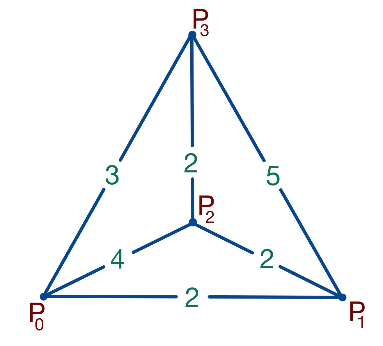
Figure 2. The fundamental $(5,3,4)$ tetrahedron.

The aim is to use $\mathbb{T}$ to explicitly writing down a RSR-representation $\rho$ that is compatible with the cocompact lattice given by the dodecahedral tiling of $\mathbb{H}^{3}.$ For computational convenience, we use the hyperboloid model of the hyperbolic 3-space. To fix notations, consider the Lorentzian space

$$\mathbb{R}^{3,1}=\left\{h=\begin{pmatrix}x_{0}+x_{1}&x_{2}+i\,x_{3}\\ x_{2}-i\,x_{3}&x_{0}-x_{1}\end{pmatrix}\,\mid\,\,\overline{h}^{T}\,=\,h\right\}$$

equipped with its canonical indefinite inner product $(.,.)$ of signature $(1,3).$ The quadratic form of $(.,.)$ is the negative of the determinant.

Then the hyperbolic 3-space is given by

$$\begin{split}\mathbb{H}^{3}&=\{(x_{0},x_{1},x_{2},x_{3})\mid-x_{0}^{2}+x_{1}^{2}+x_{2}^{2}+x_{3}^{2}=-1,\;x_{0}>0\}\\ &=\left\{h=\begin{pmatrix}x_{0}+x_{1}&x_{2}+i\,x_{3}\\ x_{2}-i\,x_{3}&x_{0}-x_{1}\end{pmatrix}\mid\;\text{det}(h)=1;\,\overline{h}^{T}=h;\,\text{Tr}(h)>0\right\}\end{split}$$ (6.1)

endowed with the Riemannian metric induced by the quadratic form $q.$ The submanifold

$$\mathbb{H}^{2}\,=\{(x_{0},x_{1},x_{2},0)\mid-x_{0}^{2}+x_{1}^{2}+x_{2}^{2}=-1,\;x_{0}>0\}$$

endowed with the induced Riemannian metric is totally geodesic and a copy of the hyperbolic 2-plane.

Recall that there exist a natural double covering of the connected component of the identity of the isometry group of $\mathbb{H}^{3}$ by SL$(2,\mathbb{C})$

$$\mathrm{SL}(2,\mathbb{C})\to\mathrm{SO}(3,1)\subset\mathrm{Isom}(\mathbb{H}^{3})$$

given by the right action

$$(h,g)\in\mathbb{H}^{3}\times\mathrm{SL}(2,\mathbb{C})\longmapsto h\cdot g=\bar{g}^{T}hg\in\mathbb{H}^{3}.$$

Restricting this map to the real subgroup $\mathrm{SL}(2,\mathbb{R})\subset\mathrm{SL}(2,\mathbb{C})$ preserves $\mathbb{H}^{2}\subset\mathbb{H}^{3}$ and defines a double covering

$$\mathrm{SL}(2,\mathbb{R})\to\mathrm{SO}(2,1)\subset\mathrm{Isom}(\mathbb{H}^{2}).$$

Consider the hyperbolic tetrahedron in $\mathbb{H}^{3}$ defined by the following 4 vertices

$$\begin{split}P_{0}&=(1,0,0,0)\\ P_{1}&=\left(\sqrt{1+\tfrac{2}{\sqrt{5}}},-\frac{1}{5^{1/4}},-\frac{1}{5^{1/4}},0\right)\\ P_{2}&=\left(\sqrt{\tfrac{1}{2}(3+\sqrt{5})},-\sqrt{\tfrac{2}{-1+\sqrt{5}}},0,0\right)\\ P_{3}&=\left(\;\tfrac{1}{2}\sqrt{7+3\sqrt{5}},-\tfrac{1}{2}\sqrt{1+\sqrt{5}},-\tfrac{1}{2}\sqrt{1+\sqrt{5}},\tfrac{1}{2}\sqrt{1+\sqrt{5}}\;\right)\end{split}$$

with (geodesic triangle) faces

$$\begin{split}&T_{0}\subset\text{span}\{P_{1},P_{2},P_{3}\}\cap\mathbb{H}^{3}\\ &T_{1}\subset\text{span}\{P_{0},P_{2},P_{3}\}\cap\mathbb{H}^{3}\\ &T_{2}\subset\text{span}\{P_{0},P_{1},P_{3}\}\cap\mathbb{H}^{3}\\ &T_{3}\subset\text{span}\{P_{0},P_{1},P_{2}\}\cap\mathbb{H}^{3}\subset\mathbb{H}^{2}.\\ \end{split}$$

Each face has a unit length normal, unique up to sign, given by

$$\begin{split}L_{0}&=\left(\,\tfrac{1}{\sqrt{1+\sqrt{5}}},-\tfrac{1}{2}\sqrt{3+\sqrt{5}},0,0\,\right)\\ L_{1}&=\left(\,0,0,\tfrac{1}{\sqrt{2}},\tfrac{1}{\sqrt{2}}\,\right)\\ L_{2}&=\left(\,0,-\tfrac{1}{\sqrt{2}},\tfrac{1}{\sqrt{2}},0\,\right)\\ L_{3}&=(\,0,0,0,1\,).\\ \end{split}$$

Computing the angles between $L_{k},$  $k=0,\,...,\,3$ the tetrahedron constructed here is in fact $\mathbb{T}$, see Figure 2. The corresponding Coexter group is generated by the reflections $R_{k}$ across the faces $T_{k}$ for $k\,=\,0,...,\,3,$ i.e.,

$$R_{k}(v)=v-2(v,L_{k})L_{k},\quad v\in\mathbb{R}^{3,1}.$$

Consider its order 2 subgroup $\mathfrak{G}$ consisting of orientation preserving transformations generated by

$$G_{m,n}:=R_{m}R_{n},\quad 0\leq m<n\leq 3.$$

We denote by $\Gamma$ the subgroup of SL$(2,\mathbb{C})$ given by the preimage of $\mathfrak{G}$ through the above double cover. Its generators are determined by choosing lifts $g_{k,l}$ of $G_{k,l}$

$$\begin{split}g_{0,1}&:=\begin{pmatrix}0&-\tfrac{1+i}{4}\left(1+\sqrt{5}+\sqrt{2(-1+\sqrt{5})}\right)\\ \frac{(2-2i)}{(1+\sqrt{5}+\sqrt{2(-1+\sqrt{5})}}&0\end{pmatrix}\\ &\\ g_{0,2}&:=\begin{pmatrix}-\tfrac{1}{2}\sqrt{1+\sqrt{5}-\sqrt{2(1+\sqrt{5})}}&\left(-\sqrt{1+\sqrt{5}-\sqrt{2(1+\sqrt{5})}}\right)^{-1}\\ \tfrac{1}{2}\sqrt{1+\sqrt{5}-\sqrt{2(1+\sqrt{5})}}&\left(-\sqrt{1+\sqrt{5}-\sqrt{2(1+\sqrt{5})}}\right)^{-1}\end{pmatrix}\\ &\\ g_{0,3}&:=\begin{pmatrix}0&-i\sqrt{\tfrac{1}{2}(1+\sqrt{5}+\sqrt{2(1+\sqrt{5})})}\\ \frac{-i}{\sqrt{\tfrac{1}{2}(1+\sqrt{5}+\sqrt{2(1+\sqrt{5})})}}&0\end{pmatrix}\\ &\\ g_{1,2}&:=\frac{1}{2}\begin{pmatrix}-1+i&1+i\\ -1+i&-1-i\end{pmatrix}\\ &\\ g_{1,3}&:=\frac{1}{\sqrt{2}}\begin{pmatrix}-1-i&0\\ 0&-1+i\end{pmatrix}\\ &\\ g_{2,3}&:=\frac{-i}{\sqrt{2}}\begin{pmatrix}1&1\\ 1&-1\end{pmatrix}.\\ \end{split}$$ (6.2)

Note that all $g_{k,l}$ are of finite order, e.g., $g_{0,2}$ is of order $5$. Consider

$$j_{0}:=g_{1,2}g_{1,3}=\frac{1}{\sqrt{2}}\begin{pmatrix}1&-1\\ 1&1\end{pmatrix}\in\text{SL}(2,\mathbb{R})$$

and

$$J_{1}:=-(g_{0,2})^{2}\in\text{SL}(2,\mathbb{R}),$$

and define

$$\begin{split}J_{2}&:=j_{0}J_{1}j_{0}^{-1}\\ J_{3}&:=j_{0}J_{2}j_{0}^{-1}\\ J_{4}&:=j_{0}J_{3}j_{0}^{-1}.\\ \end{split}$$ (6.3)

Note that $j_{0}$ is of order 8 and $J_{1},\dots,J_{4}$ are all of order 10. A direct computation then shows

$$J_{4}J_{3}J_{2}J_{1}=\text{Id}.$$

Theorem 6.1.

The representation $\rho\,\colon\,\pi_{1}(S_{4},\,s_{0})\,\longrightarrow\,\text{SL}(2,\mathbb{C})$ of the 4-punctured sphere $S_{4}$ given by

$$\rho(\gamma_{k})\,=\,J_{k}$$

is a genus $4$ RSR-representation compatible with the cocompact lattice $\Gamma\subset\mathrm{SL}(2,\mathbb{C}).$

Proof.

The group $\Gamma$ (the preimage of $\mathfrak{G}$) is a cocompact lattice of $\mathrm{SL}(2,\mathbb{C})$, since it corresponds (up to a reflection) to the tessellation of $\mathbb{H}^{3}$ by copies of the tetrahedron $\mathbb{T}$. Since $J_{k}$ lies in SL$(2,\mathbb{R})$ for all $k\,=\,1,\,\cdots,\,4$, and

$$\text{tr}(J_{2}J_{1})=\text{tr}(J_{3}J_{2})=-1-\sqrt{5}<-2,\quad\text{tr}(J_{3}J_{1})=-\tfrac{3}{2}(1+\sqrt{5})<-2,$$

the image of the representation $\rho$ defines a real lattice $\widehat{\Gamma}$ in $\mathrm{SL}(2,\mathbb{R})$. Moreover, $\widehat{\Gamma}$ is symmetric with $\widetilde{r}=\tfrac{3}{10}\in(\tfrac{1}{4},\tfrac{1}{2})$, since

$$\text{tr}(J_{k})=\frac{1}{2}(1-\sqrt{5})=2\cos\left(2\pi\tfrac{3}{10}\right)\quad\text{for}\quad k=1,...,4,$$

and rectangular by

$$\text{tr}(J_{3}J_{1})\,=\,\text{tr}(J_{4}J_{2})\,=\,-\tfrac{3}{2}(1+\sqrt{5}).$$

Since the order of the $J_{j}$ is 10, the genus of the representation is $4$ by Definition 2.2. ∎

Applying Theorem 2.4 we obtain:

Corollary 6.2.

There exist a cocompact lattice $\Gamma$ in $\mathrm{SL}(2,\mathbb{C})$ and a compact Riemann surface $\Sigma$ of genus $g=4$ admitting a holomorphic map $f\colon\Sigma\to\mathrm{SL}(2,\mathbb{C})/\Gamma$ which does not factor through a curve of lower genus.

6.1. Outlook: CMC 1 surfaces in hyperbolic 3-manifolds

Surfaces with constant mean curvature $H$ in Riemannian 3-manifolds are the critical points of the area functional with fixed enclosed volume. By the Lawson correspondence [La], CMC 1 surfaces (i.e., surfaces with $H=1$) in hyperbolic 3-space are (locally) in one-to-one correspondence with minimal surfaces in $\mathbb{R}^{3}.$ The latter can be explicitly parametrized in terms of holomorphic data by the classical Weierstrass representation.

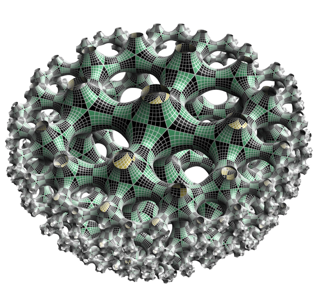
Figure 3. An equivariant CMC 1 surface compatible with the dodecahedron tesselation of $\mathbb{H}^{3}$. The shown lines are the trajectories of a holomorphic quadratic differential of the underlying compact Riemann surface of genus 3. Image by Nick Schmitt.

As first noticed by Bryant [Bry], see also [UY], there exists a local Weierstrass representation of CMC 1 surfaces in $\mathbb{H}^{3}$ as well. Consider for this a nilpotent nowhere vanishing $\mathfrak{sl}(2,\mathbb{C})$-valued holomorphic 1-form $\Phi$ on a Riemann surface $\Sigma.$ The frame $F$ is a solution of the ordinary differential equation $dF=\Phi F$. Then the conformal immersion $f$ (defined on the universal covering of $\Sigma$) given by $f=\bar{F}^{T}F$ has constant mean curvature $1$ in the hyperbolic 3-space. In invariant terms, every CMC 1 surface is given by a flat unitary connection $\nabla$ together with a nilpotent Higgs field $\Phi,$ see [Pi]. The frame $F$ is then a parallel frame with respect to the flat connection $\nabla-\Phi.$ The unitary connection $\nabla$ gives rise to an associated flat unitary bundle $V\rightarrow\Sigma$ whose transition functions are determined by the local unitary frames of $\nabla.$ Since the representation formula is not sensitive with respect to appropriate changes of the parallel unitary frames, the choice of the unitary frame does not alter the CMC 1 immersion. We say a CMC 1 surface in a hyperbolic manifold admits a simple Weierstrass representation, if the corresponding flat unitary bundle is trivial. The following theorem holds.

Theorem 6.3.

A CMC 1 surface $f\colon\Sigma\to\mathbb{H}^{3}/\Gamma$ into a hyperbolic 3-manifold $\mathbb{H}^{3}/\Gamma$ admits a simple Weierstrass representation if and only if it is the projection of a holomorphic curve $F\colon\Sigma\to\mathrm{SL}(2,\mathbb{C})/\Gamma.$

Even though we have shown the existence of holomorphic curves into $\mathrm{SL}(2,\mathbb{C})/\Gamma$ where $\Gamma$ is the dodecahedron tesselation group, and there exists compact CMC 1 surfaces in $\mathbb{H}^{3}/\Gamma$, see Figure 3, it is unclear whether there exist compact CMC 1 surfaces in $\mathbb{H}^{3}/\Gamma$ with simple Weierstrass representation, since the Higgs fields of the holomorphic curves we constructed here are not nilpotent.

References

• [At] M. F. Atiyah, Riemann surfaces and spin structures, Ann. Sci. Ecole Norm. Sup. (4) 4 (1971), 47–62.
• [BeG] R. L. Benedetto and W. Goldman, The Topology of the Relative Character Varieties of a Quadrupuly-Punctured Sphere, Experimental Math. 8(1) (1999), 85–103.
• [Be] L. A. Best, On torsion-free discret subgroups of $\text{PSL}(2,\mathbb{C})$ with compact orbit space, Can. J. Math. XXIII(3) (1971), 451–460.
• [Biq] O. Biquard, Fibrés paraboliques stables et connexions singulières plates, Bull. Soc. Math. Fr. 119 (1991), 231–257.
• [BD] I. Biswas and S. Dumitrescu, Riemann-Hilbert correspondence for differential systems over Riemann surfaces, arxiv.org/abs/2002.05927.
• [BDH] I. Biswas and S. Dumitrescu and S. Heller, Irreducible flat ${\rm SL}(2,\mathbb{R})$-connections on the trivial holomorphic bundle, J. Math. Pures Appl. 149 (2021), 28–46.
• [BDHH] I. Biswas and S. Dumitrescu, L. Heller and S. Heller, Fuchsian $sl(2,\mathbb{C})$-systems of compact Riemann surfaces (with an appendix by Takuro Mochizuki), arxiv.org/abs/2104.04818.
• [Bob] A.I. Bobenkos, Surfaces in terms of 2 by 2 matrices. Old and new integrable cases, In: A.P. Fordy, J.C. Wood (eds.) ”Harmonic Maps and Integrable Systems”, Vieweg, Braunschweig/Wiesbaden 1994, pp. 81–127.
• [Bry] R. Bryant, Surfaces of mean curvature one in hyperbolic space. Theorie des varietes minimales et applications (Palaiseau, 1983-1984), Asterisque No. 154–155 (1987), 12, 321–347, 353 (1988).
• [Bu] P. Buser, Geometry and Spectra of Compact Riemann Surfaces, Modern Birkhäuser Classics, Boston, Birkhäuser, 1992.
• [CDHeL] G. Calsamiglia, B. Deroin, V. Heu and F. Loray, The Riemann-Hilbert mapping for $sl(2)$-systems over genus two curves, Bull. Soc. Math. France 147 (2019), 159–195.
• [Co1] H.S.M. Coxeter, Regular Polytopes, Methuen & Co. Ltd., London, (1948;1949); Third Edition, Dover, New York, (1973).
• [Co2] H.S.M. Coxeter, Regular honeycombs in hyperbolic spaces, Proceedings I.C.M. (Amsterdam, 1954), vol. III, pp. 155–169, Erven P. Noordhoff N.V., Groningen, (1956).
• [De] P. Deligne, Equations différentielles à points singuliers réguliers, Lecture Notes in Mathematics, Vol. 163, Springer-Verlag, Berlin-New York, 1970.
• [Falt] Gerd Faltings, Real projective structures on Riemann surfaces, Compositio Math. 48 (1983), 223–269.
• [Gh] E. Ghys, Déformations des structures complexes sur les espaces homogènes de ${\rm SL}(2,\mathbb{C})$, Jour. Reine Angew. Math. 468 (1995), 113–138.
• [Go87] W. M. M. Goldman, Projective structures with Fuchsian holonomy, J. Differential Geom. 25 (1987), 297–326.
• [Go88] W. M. Goldman, Topological components of spaces of representations, Invent. Math. 93 (1988), 557–607.
• [Go97] W. M. Goldman, Ergodic Theory on Moduli Spaces, Ann. of Math. (2), 146, pp. 475–507 (1997).
• [Go03] W. M. Goldman, The modular group action on real $\mathrm{SL}(2)$-characters of a one-holed torus, Geometry $\&$ Topology Volume 7 (2003) 443–486.
• [Gu] R. C. Gunning, Lectures on vector bundles over Riemann surfaces, University of Tokyo Press, Tokyo; Princeton University Press, Princeton, (1967).
• [Gu1] R. C. Gunning, On uniformization of complex manifolds: the role of connections, Princeton Univ. Press, 1978.
• [Hej] D. A. Hejhal, Monodromy groups and linearly polymorphic functions, Acta Math. 135 (1975), 1–55.
• [HH] L. Heller and S. Heller, Abelianization of Fuchsian systems and Applications, Jour. Symp. Geom. 14 (2016), 1059–1088.
• [HHSch] L. Heller, S. Heller, N. Schmitt, Navigating the space of symmetric cmc surfaces Journal of Differential Geometry, Vol. 110, No. 3 (2018), pp. 413–455.
• [HM] A. H. Huckleberry and G. A. Margulis, Invariant Analytic hypersurfaces, Invent. Math. 71 (1983), 235–240.
• [HW] A. H. Huckleberry and J. Winkelmann, Subvarieties of parallelizable manifolds, Math. Ann. 295 (1993), 469–483.
• [John] D. Johnson, Spin structures and quadratic forms on surfaces, J. LMS (2), 22 (1980), 365–373
• [La] H.B: Lawson, Complete minimal surfaces in $S^{3}$, Ann. of Math. (2) 92 (1970), 335–374.
• [Lo] F. Loray, Isomonodromic deformations of Lamé connections, the Painlevé VI equation and Okamoto symmetry, Izv. Ros. Acad. Nauk. Ser. Math 80(1) (2016), 119–176.
• [Mas] B. Maskit, On a class of Kleinian groups, Ann. Acad. Sci. Fenn., Ser. A I No. 442 (1969), 8.
• [MS] V. B. Mehta and C. S. Seshadri, Moduli of vector bundles on curves with parabolic structures, Math. Ann. 248 (1980), 205–239.
• [MY] M. Maruyama and K. Yokogawa, Moduli of parabolic stable sheaves, Math. Ann. 293 (1992), 77–99.
• [P] U. Pinkall, Regular homotopy classes of immersed surfaces, Topology 24 (1985), 421–434.
• [Pi] G. Pirola, Monodromy of constant mean curvature surface in hyperbolic space, Asian Jour. Math. 11 (2007), 651–669.
• [NS] M. S. Narasimhan and C. S. Seshadri, Stable and unitary bundles on a compact Riemann surface, Ann. of Math. 82 (1965), 540–564.
• [Ra] J.G. Ratcliffe, Foundations of Hyperbolic Manifolds, Graduate Texts in Math., Third Edition, Springer Nature Switzerland AG, (1994, 2006,2019)
• [Si1] C. T. Simpson, Harmonic bundles on noncompact curves, Journal of the AMS, Volume 3, July 1990.
• [ST] D. Sullivan and W. Thurston, Manifolds with canonical coordinate charts: some examples, Enseign. Math. (2) 29 (1983), no. 1-2, 15–25.
• [Tak] L. A. Takhtajan, Real projective connections, V. I. Smirnov’s approach, and black-hole-type solutions of the Liouville equation, Theoret. and Math. Phys. 181 (2014), no. 1, 1307–1316, Russian version appears in Teoret. Mat. Fiz. 181, (2014), no. 1, 206–217.
• [Tan] H. Tanigawa, Grafting, harmonic maps and projective structures on surfaces, J. Differential Geom. 47 (1997), no. 3, 399–419.
• [Th] W. Thurston, Three dimensional manifolds, Kleinian groups and hyperbolic geometry, Bull. Amer. Math. Soc. 6 (1982), 357–381.
• [UY] M. Umehara and K. Yamada, Complete surfaces of constant mean curvature 1 in the hyperbolic 3-space, Ann. of Math. (2) 137 (1993), no. 3, 611–638.
• [Wa] H.-C. Wang, Complex Parallelisable manifolds, Proc. Amer. Math. Soc. 5 (1954), 771–776.