Estimation and reduced bias estimation of the residual dependence index with unnamed marginals

Abstract

Unlike univariate extreme value theory, multivariate extreme value distributions cannot be specified through a finite-dimensional parameter family of distributions. Instead, the many facets of multivariate extremes are mirrored in the inherent dependence structure of component-wise maxima which must be dissociated from the limiting extreme behaviour of its marginal distribution functions before a probabilistic characterisation of an extreme value quality can be determined. Mechanisms applied to elicit extremal dependence typically rely on standardisation of the unknown marginal distribution functions from which pseudo-observations for either Pareto or Fréchet marginals result. The relative merits of both of these choices for transformation of marginals have been discussed in the literature, particularly in the context of domains of attraction of an extreme value distribution. This paper is set within this context of modelling penultimate dependence as it proposes a unifying class of estimators for the residual dependence index that eschews consideration of choice of marginals. In addition, a reduced bias variant of the new class of estimators is introduced and their asymptotic properties are developed. The pivotal role of the unifying marginal transform in effectively removing bias is borne by a comprehensive simulation study. The leading application in this paper comprises an analysis of asymptotic independence between rainfall occurrences originating from monsoon-related events at several locations in Ghana.

KEY WORDS AND PHRASES: Asymptotic independence, extreme value distribution, Hill estimator, monsoon season, rainfall in Ghana, regular variation, semi-parametric estimation, tail copula.

1 Introduction

Statistical methodology for inference drawing on multivariate extremes has garnered considerable interest from the standpoint of the many challenges faced by applied scientists when attempting to model extreme and perilous events in the midst of a rapidly changing 21${}^{\textrm{th}}$ century. This paper is motivated by an applied study emerging from the need for a better understanding to be gained of the extent at which spatial dependence in tropical rainfall occurrences can manifest itself at extreme levels. The significance of such a study, as well as its relevance, has been highlighted in a body of published research. Notably, Sang and Gelfand, (2009) argue that an asymptotically independent model should be considered due to the convective nature of extreme tropical precipitation.

The foundational stream to the extreme value statistical analysis in this paper is concerned with estimating penultimate extremal dependence between two random variables, within which context we tackle the problem of reduced bias estimation for the residual dependence index. The residual dependence index, aka coefficient of tail dependence or residual dependence coefficient was introduced by Ledford and Tawn, (1996) and further investigated by Ramos and Ledford, (2009), Haan and Zhou, (2011) and Eastoe and Tawn, (2012).

Let $(X_{i},Y_{i})$, $i=1,...,n$, be independent copies of the random vector $(X,Y)$ with joint distribution function $F$ whose marginal distributions we denote by $F_{1}$ and $F_{2}$, i.e. $F_{1}(x):=F(x,\infty)$ and $F_{2}(y):=F(\infty,y)$, assumed continuous. The interest is in evaluating the probability of the two components being large at the same time, more formally that $P(X>u_{1}\mbox{ and }Y>u_{2})$, for large $u_{1},u_{2}$, usually much larger than their respective sample maxima $\max(X_{1},\ldots,X_{n})$ and $\max(Y_{1},\ldots,Y_{n})$ in the component-wise sense. More concretely, this paper is concerned with the near-zero probability of joint exceedances against the backdrop of asymptotic independence. In environmental science, for example, this can describe the situation of two different variables being large at the same time, for example strong wind-speeds and extreme wave heights, or two large events in relation to the same process occurring at nearby locations, for example heavy rainfall at two neighbouring cities. Since we are restricting focus on the largest values, extreme value theory for threshold exceedances is the right theory to rely upon.

1.1 Background

We assume that the identically distributed random pairs $(X_{1},Y_{1}),\ldots,(X_{n},Y_{n})$ have common distribution function $F$ which belongs to the domain of attraction of a bivariate extreme value distribution. That is, there exist constants $a_{n},c_{n}>0$ and $b_{n},d_{n}\in\real$ such that, for all continuity points $(x,y)$ of $G$ the following limit relation involving the component-wise partial maxima, $M_{X,n}=\max(X_{1},\ldots,X_{n})$ and $M_{Y,n}=\max(Y_{1},\ldots,Y_{n})$, is satisfied:

$${\lim_{n\rightarrow{\infty}}}P\left(\frac{M_{X,n}-b_{n}}{a_{n}}\leq x,\frac{M_{Y,n}-d_{n}}{c_{n}}\leq y\right)=\displaystyle{\lim_{n\rightarrow{\infty}}}F^{n}(a_{n}+b_{n}x,\,c_{n}+d_{n}y)=G(x,y).$$ (1)

The domain of attraction condition (1) implies convergence of the marginal distributions to the corresponding $G(x,\infty)$ and $G(\infty,y)$ limits, whereby it is possible to redefine the constants $a_{n},c_{n},b_{n},d_{n}$ in such a way that both $G(x,\infty)=\exp\bigl{\{}-(1+\gamma_{1}x)^{-1/\gamma_{1}}\bigr{\}}=:G_{1}(x)$ and $G(\infty,y)=\exp\bigl{\{}-(1+\gamma_{2}y)^{-1/\gamma_{2}}\bigr{\}}=:G_{2}(y)$ are attained, thus laying out $\gamma_{1}$ and $\gamma_{2}$ as the extreme value indices of the marginal distributions (generalised extreme value marginals with $\gamma_{1},\gamma_{2}\in\real$, respectively). Additionally, in order to formulate a suitable condition regarding extremal dependence, we define the marginal tail quantile functions $U_{i}:=\bigl{(}1/(1-F_{i})\bigr{)}^{\leftarrow}$, $i=1,2$, where ^← indicates the generalised inverse function. By virtue of Theorem 6.2.1 of de Haan and Ferreira, (2006), it is possible to replace $n$ with $t$ running over the real line, thus enabling a slight generalisation of condition (1): with $G_{0}(x,y):=G\bigl{(}(x^{\gamma_{1}}-1)/\gamma_{1},\,(y^{\gamma_{2}}-1)/\gamma_{2}\bigr{)}$, for any $(x,\,y)$ such that $0<G_{0}(x,y)<1$,

$${\lim_{t\rightarrow{\infty}}}\frac{1-F\bigl{(}U_{1}(tx),U_{2}(ty)\bigr{)}}{1-F\bigl{(}U_{1}(t),U_{2}(t)\bigr{)}}=\frac{-\log G_{0}(x,y)}{-\log G_{0}(1,1)}=:\Psi(x,y).$$ (2)

We note that $-\log G_{1}(x)=-\log G_{2}(x)=1/x$, $x>0$. Hence, the above extreme value condition essentially ascertains that transformation of the marginal distributions to standard Pareto, with tail distribution function $1-F(t)=(t^{-1}\wedge 1)$, makes it possible to eschew the influence of the margins and move on to drawing extreme behaviour from the dependence structure alone. Without loss of generality, we proceed with the characterisation for domains of attraction aiming at the limiting class of distributions $-\log G_{0}$. We also note that analogous characterisation for the joint tail behaviour in (2), but by restricting focus to the class of simple max-stable distributions $G_{0}$ (i.e. with fixed unit Fréchet marginals) is presented in Di Bernardino et al., (2013). Other marginal standardisations in relation to the definition of different dependence structures in extremes are presented in Sections 8.2 and 8.3 of Beirlant et al., (2004).

As well as noting that, since $\Psi$ is homogeneous of order $-1$, condition (2) implies that $1-F\bigl{(}U_{1}(t),U_{2}(t)\bigr{)}$ is of regular variation at infinity with index $-1$ (i.e. $\lim_{t\rightarrow\infty}\bigl{\{}1-F\bigl{(}U_{1}(tx),U_{2}(tx)\bigr{)}\bigr{\}}/\bigl{\{}1-F\bigl{(}U_{1}(t),U_{2}(t)\bigr{)}\bigr{\}}=\Psi(x,x)=x^{-1}\Psi(1,1)=x^{-1}$, for all $x>0$), it is worth highlighting that (2) (and hence (1) with the marginals of $G$ standardised as $G_{1}$ and $G_{2}$) implies the domain of attraction condition on the basis of the tail copula:

$$\lim_{t\downarrow 0}t^{-1}P\bigl{(}1-F_{1}(X)<tx,\,1-F_{2}(Y)<ty\bigr{)}$$ (3)

$$= \frac{1}{x}+\frac{1}{y}-\displaystyle{\lim_{t\rightarrow{\infty}}}tP\Bigl{(}X>U_{1}\bigl{(}tx\bigr{)}\mbox{ or }Y>U_{2}\bigl{(}ty\bigr{)}\Bigr{)}=\frac{1}{x}+\frac{1}{y}+\log G_{0}(x,y),$$ (4)

for all $x,y>0$ such that $0<G_{0}(x,y)<1$. The extreme value dependence structure is brought through in terms of combined tail regions $U_{j}(t\,\centerdot)$, $j=1,2$, expressed in (4), for sufficiently large $t$. In particular, if the underlying distribution function $F$ is in the domain of attraction of a bivariate extreme value distribution with independent components, i.e., $F$ is such that (2) holds with $\log G_{0}(x,y)=\log G_{1}(x)+\log G_{2}(y)$, then the random pair $(X,Y)$ is said to be asymptotically independent, and the limit above results in zero. This paper is set within the context of asymptotic independence that will eventually render the tail copula condition, condition (4), useless for the purposes of inference in the two-dimensional framework for extremes. There are numerous distributions possessing the asymptotic independence property, most notably the bivariate normal with correlation coefficient $\rho<1$, an example worked out by Sibuya, (1960). We also refer to Heffernan, (2000) in this respect. Seminal works by Ledford and Tawn, (1996, 1997) exploit the asymptotically independent case in such as way as to define an appropriate sub-model whereby $P\bigl{(}1-F_{1}(X)<t\mbox{ or }1-F_{2}(Y)<t\bigr{)}$ is regularly varying at zero with index $1$ and $P\bigl{(}1-F_{1}(X)<t,\,1-F_{2}(Y)<t\bigr{)}$ is regularly varying at zero with index $1/\eta$ greater than or equal to one. Hence, the residual dependence index terminology for $\eta\in(0,\,1]$ (cf. de Haan and Ferreira,, 2006, Section 7.6). A considerable body of literature on the estimation of $\eta$ is available to date, of which perhaps the best aligned with the angle taken in this paper are the works by Draisma et al., (2004); Goegebeur and Guillou, (2012).

1.2 Our contribution

It is the aim of this paper to introduce a broad class of estimators for the residual dependence index $\eta$ which includes the widely used Hill estimator (Hill,, 1975) for the tail index. We devise a way of circumventing potential differences between transformation of marginals to standard Pareto or unit Fréchet that have been widely reported in the literature, thus rendering a seamless framework for tackling the challenge of bias reduction in the estimation of $\eta$ (cf. Di Bernardino et al.,, 2013; Draisma et al.,, 2004). Our numerical results demonstrate that it is not always the case that estimators for the residual index upon Fréchet standardisation exhibit larger bias than those stemming from standardisation to Pareto marginals. Simply through a simple shift of unit Fréchet pseudo-observations by $1/2$, our proposed class of estimators is able to offset against the caveat highlighted in Goegebeur and Guillou, (2012, point(i), Section 4.3), for example, that “The Hill estimator is generally biased, though the bias seems to be a more severe problem for unit Fréchet marginal distributions than for unit Pareto marginal distributions”. In a similar vein, (Draisma et al.,, 2004, page 254) hints at lower bias whenever the Pareto transformation is employed as opposed to the unit Fréchet, a problem which is also curbed with our approach, albeit their remark may well be grounded in the asymptotic properties of the maximum likelihood estimator for the tail index in relation to a heavy-tailed univariate distribution.

1.3 Organisation of the paper

The remainder of this paper is organised as follows. Section 2 is devoted to our proposed class of estimators for $\eta\in(0,1]$ and its asymptotic properties of consistency and asymptotic normality are developed in Section 3. We then go on to study in detail particular members (estimators) within this class of estimators for the residual dependence index $\eta$ which we found most promising, and devise an associated reduced bias class of estimators for $\eta$. This is presented in Section 4. All necessary proofs to the main results presented in Sections 3 and 4 are deferred to Section 5. Section 6 contains simulation results for evaluating finite sample performance of representative estimators for the proposed classes of estimators in Section 2 and their reduced bias variants encompassing Section 4. Complementary simulation results can be found in Appendices A and B. Finally, in Section 7, the new estimators for the residual dependence index are applied to daily tropical rainfall data, collected across a highly dense network of gauging stations in Ghana.

2 Estimation of the residual dependence index

We assume that $F$ is in the domain of attraction of an extreme value distribution, that is, $F$ satisfies the domain of attraction condition (1). Since the focus is on the asymptotic independence property, the primary assumption to our results is the analogue of (2) in terms of the tail copula (3): for $x,\,y>0$,

$$\lim_{t\downarrow 0}\frac{P\bigl{(}1-F_{1}(X)<tx,\,1-F_{2}(Y)<ty\bigr{)}}{P\bigl{(}1-F_{1}(X)<t,\,1-F_{2}(Y)<t\bigr{)}}=:S(x,y)$$ (5)

exists and is positive. Then $q(t):=P\bigl{(}1-F_{1}(X)<t,\,1-F_{2}(Y)<t\bigr{)}$ is regularly varying at zero with index $1/\eta$, i.e., $\lim_{t\downarrow 0}q(tx)/q(t)=x^{1/\eta}$, for some $\eta\in(0,1]$. Without loss of generality, we put $x=y$ in (5). Then, heeding the development in (4), we find that the left hand-side of (5) is, in a certain sense, proportional to $\lim_{t\downarrow 0}t^{-1}q(t)=l$, which we assume exists and is finite in order to ensure the domain of attraction condition holds. If there is no asymptotic independence, then $\eta$ must be equal to one in order that $l>0$ (in fact $0<l\leq 1$, since $\limsup_{t\rightarrow 0}t^{-1}q(t)\leq 1$ as both $1-F(X_{1})$ and $1-F(X_{2})$ are uniformly distributed). If $\eta<1$ then $l=0$ and there is asymptotic independence. However, $\eta=1$ does not guarantee asymptotic dependence. Similarly as before, condition (2) implies

$${\lim_{t\rightarrow{\infty}}}\frac{P\Bigl{(}\frac{1}{1-F_{1}(X)}\wedge\frac{1}{1-F_{2}(Y)}>tx\Bigr{)}}{P\Bigl{(}\frac{1}{1-F_{1}(X)}\wedge\frac{1}{1-F_{2}(Y)}>t\Bigr{)}}=S\Bigl{(}\frac{1}{x},\frac{1}{x}\Bigr{)}=x^{-1/\eta}S(1,1)=x^{-1/\eta},$$ (6)

for all $x>0$. That is, the tail distribution function (aka survival function) $\overline{F}_{T}:=1-F_{T}$ of the random variable $T:=\bigl{\{}\bigl{(}1-F_{1}(X)\bigr{)}\vee\bigl{(}1-F_{2}(Y)\bigr{)}\bigr{\}}^{-1}$ is regularly varying at infinity with index $-1/\eta$. As highlighted in de Haan and Ferreira, (2006, p. 265), this enables a Hill-type estimator to be used for tackling the problem of estimating the residual dependence index $\eta\in(0,\,1]$. Unless both marginal distributions $F_{1}$ and $F_{2}$ are known, the variable $T$ cannot be observed. However, consistent estimation is achieved through the corresponding empirical distribution functions thus resulting in the pseudo-observables of $T$, defined by:

$$T_{i}^{(n)}:=\frac{n+1}{n+1-R(X_{i})}\wedge\frac{n+1}{n+1-R(Y_{i})},$$ (7)

where $R(X_{i})$ stands for the rank of $X_{i}$ among $(X_{1},X_{2},\ldots,X_{n})$, that is , $R(X_{i}):=\sum_{j=1}^{n}\mathds{1}_{\{X_{j}\leq X_{i}\}}$, and $R(Y_{i})$ is the rank of $Y_{i}$ among $(Y_{1},Y_{2},\ldots,Y_{n})$. Hence, $\bigl{\{}T_{i}^{(n)}\bigr{\}}_{i=1}^{n}$ consists of a sequence of non-independent and identically distributed random variables associated with $T$, whose ascending order statistics we denote by $T_{n,1}\leq T_{n,2}\leq\ldots\leq T_{n,n}$. Since the marginal distribution functions are unknown, thus needing to be estimated whilst the limit $S(x,x)$ in (5) is completely specified up to one parameter (notably the residual tail index $\eta\in(0,1]$), our proposed inference takes place in a semi-parametric setting.

With $Q_{n}(s):=T_{n,n-[ms]}$, for $0<s<n/m$, the tail empirical quantile function of $T_{i}^{(n)}$, we note that $(m/n)Q_{n}(1)\,\displaystyle{\mathop{\longrightarrow}^{P}}\,\,l$, with $l$ positive, as $m\rightarrow\infty$, whereas for an intermediate sequence of positive integers $k(n)=nq^{\leftarrow}(m/n)\rightarrow\infty$, $k/n\rightarrow 0$, as $n\rightarrow\infty$, it results that $(k/n)Q_{n}(1)\,\displaystyle{\mathop{\longrightarrow}^{P}}\,1$ (cf. Goegebeur and Guillou,, 2012). Our proposed class of estimators for the residual dependence index $\eta$ then builds on the functional

$$M_{a,b}(z):=\frac{\bigl{(}A_{a}(z)\bigr{)}^{b}-1}{b},\quad\mbox{ with }A_{a}(z):=\biggl{\{}\int_{0}^{1}\Bigl{(}\frac{z(s)}{z(1)}\Bigr{)}^{a}\,ds\biggr{\}}^{1/a},\;a,b\in\real,$$ (8)

with a measurable function $z:[0,1]\rightarrow\real$. The case of $a=0$ and/or $b=0$ is interpreted in the limiting sense as $\log z$, leading to the celebrated Hill estimator by means of the functional

$$M_{0}(z):=\int_{0}^{1}\log\frac{z(s)}{z(1)}\,ds.$$ (9)

Under suitable conditions involving a second order refinement of (5), $M_{a,b}\bigl{(}Q_{n}\bigr{)}(s)$ yields a new class of consistent asymptotically normal estimators for the residual dependence index $\eta$, provided $a/b$ is set (fixed) at approximately $-1$. This will be established in Section 3. The primary estimator in this paper originates from (8) through a suitable choice for the $(a,b)$-pair, namely $(p^{-1},q^{-1}-1)$ with conjugate constants $p\in\real$, $q>0$, that is, $1/p+1/q=1$. Specifically,

$$\hat{\eta}_{q}(k):=\frac{\biggl{\{}\Bigl{[}\frac{1}{k}\sum\limits_{i=0}^{k-1}\Bigl{(}\frac{T_{n,n-i}}{T_{n,n-k}}\Bigr{)}^{\frac{1}{p}}\Bigr{]}^{p}\biggr{\}}^{-(1-1/q)}-1}{-(1-1/q)}.$$ (10)

Setting $q=1$ in the above allows us to recover the Hill estimator as in (9). Moreover, $M_{a,b}\bigl{(}Q_{n}(s)\bigr{)}$ with $a=1/(1-p)$ and $b=q-1$ renders the “mean-of-order-$p$” estimator presented in Gomes et al., (2015), which approaches (10) at its place of confluence with the Hill estimator, i.e., for $q=1$. Some simulation results for this estimator are presented in Appendix B.

To estimate the residual dependence index $\eta$, we firstly consider the marginals’ transformation to the standard Pareto distribution as advocated in Draisma et al., (2004). Secondly, the relevant sequence of random variables to this same purpose of estimating the residual dependence index is derived by drawing on unit Fréchet transformation of marginals in a similar way as before (see also Goegebeur and Guillou,, 2012; Di Bernardino et al.,, 2013). Again, since $F_{1}$ and $F_{2}$ are unknown continuous distribution functions, we are going to replace these with their corresponding empirical distribution functions $F_{1}^{(n)}$ and $F_{2}^{(n)}$, respectively, on the basis of the customary plotting positions $i/(n+1)$ to avoid division by 0. This results in the sequence $\big{\{}V_{i}^{(n)}\bigr{\}}_{i=1}^{n}$ of a non-independent and identically distributed sequence of pseudo-observables:

$$V_{i}^{(n)}:=\biggl{(}-\frac{1}{\text{log }F_{1}^{(n)}(X_{i})}\biggr{)}\wedge\biggl{(}-\frac{1}{\text{log }F_{2}^{(n)}(Y_{i})}\biggr{)}=\Bigl{\{}\Bigl{(}-\log\frac{R(X_{i})}{n+1}\Bigr{)}\vee\Bigl{(}-\log\frac{R(Y_{i})}{n+1}\Bigr{)}\Bigr{\}}^{-1}.$$ (11)

We denote by $V_{n,1}\leq\ldots\leq V_{n,n}$, the associated order statistics and consider the counterparts to estimators encapsulated in (8), with particular focus in the primary $\hat{\eta}_{q}(k)$ (as in (10)) through pseudo unit Fréchet random variables, upon a location-shift by $1/2$. In other words, we consider the class of location-shifted estimators for $\eta$, defined as:

$$\hat{\eta}_{a,b}^{(S)}(k):=\frac{\biggl{\{}\Bigl{[}\frac{1}{k}\sum\limits_{i=0}^{k-1}\Bigl{(}\frac{1/2+V_{n,n-i}}{1/2+V_{n,n-k}}\Bigr{)}^{a}\Bigr{]}^{1/a}\biggr{\}}^{b}-1}{b},$$ (12)

thus ascribed to the functional $M_{a,b}\bigl{(}V_{n,n-[ms]}+1/2\bigr{)}$, with $a/b\rightarrow-1$ via conjugate constants $p\in\real$, $q>0$. All the asymptotic results pertaining to the class (12) are established in the next section. This includes a theorem establishing that estimators $\hat{\eta}_{a,b}^{(S)}$, which the proposed class (12) of shifted estimators for the residual dependence index $\eta\in(0,1]$ embodies, are asymptotically equivalent to their canonical versions $\hat{\eta}_{a,b}=M_{a,b}\bigl{(}Q_{n}\bigr{)}$ on the basis of the transformation to standard Pareto margins. Our numerical simulations in Section 6 demonstrate that any initial choice of $q$ near 1, albeit different to 1, can yield substantial reduction in the finite sample bias.

3 Asymptotic results

In order to derive the asymptotic distribution of the class of estimators $M_{a,b}(k)$ in the two-dimensional setting for extremes, a second order refinement of (5) is required (see Draisma et al.,, 2004; Goegebeur and Guillou,, 2012). Hence, we assume in addition that $S$ is continuously differentiable,

$$\lim\limits_{t\downarrow 0}\frac{\frac{P(1-F_{1}(X)<tx,1-F_{2}(Y)<ty)}{q(t)}-S(x,y)}{q_{1}(t)}=:D(x,y)$$ (13)

exists for all $x,y\geq 0$, $x+y>0$, with $q_{1}$ of ultimately constant sign and tending to 0 as $t\downarrow 0$ and a function $D$ which is neither constant nor a multiple of $S$. We assume that the convergence is uniform on $\{(x,y)\in[0,\infty)^{2}$ $|$ $x^{2}+y^{2}=1\}$, and that $D(x,x)=x^{1/\eta}\frac{x^{\tau/\eta}-1}{\tau\eta}$. We note that, in addition to the function $q$ being of regular variation at 0 with index $1/\eta$, condition (13) implies that $|q_{1}|$ is regularly varying with index $\tau/\eta\geq 0$. Moreover, we assume that $l:=\lim_{t\downarrow 0}q(t)/t$ exists. The latter is always satisfied if $\eta<1$ or $\tau>0$. We refer to Goegebeur and Guillou, (2012) in this respect. Assumption (13) and the stated additional conditions encompass the standard requirement for the asymptotic normality to be attained by existing estimators of the residual dependence index.

Theorem 1

Let $T_{n,1}\leq T_{n,2}\leq\ldots\leq T_{n,n}$ be the ascending order statistics associated with the identically distributed random variables $T_{i}^{(n)}$, $i=1,2,\ldots,n$ defined in (7), with tail distribution function $\overline{F}_{T}:=1-F_{T}$ satisfying (6). Assume the following second order condition of regular variation for $\overline{F}_{T}$, which is implied by (13) and its inherent assumptions: there exist $\eta\in(0,1]$, $\tau>0$ and a function $q_{\star}(t)\rightarrow 0$, as $t\rightarrow\infty$, not changing sign eventually such that, for all $x>0$,

$${\lim_{t\rightarrow{\infty}}}\,\frac{\frac{P\Bigl{(}\frac{1}{1-F_{1}(X)}\wedge\frac{1}{1-F_{2}(Y)}>tx\Bigr{)}}{\overline{F}_{T}(t)}-x^{-1/\eta}}{q_{\star}\bigl{(}\nicefrac{{1}}{{\overline{F}_{T}(t)}}\bigr{)}}=x^{-1/\eta}\frac{x^{-\tau/\eta}-1}{\eta\tau}.$$

Assume the equivalent relation in terms of high quantiles:

$${\lim_{t\rightarrow{\infty}}}\frac{\nicefrac{{\bigl{(}\frac{1}{1-F_{T}}\bigr{)}^{\leftarrow}(tx)}}{{\bigl{(}\frac{1}{1-F_{T}}\bigr{)}^{\leftarrow}(t)}}-x^{\eta}}{q_{\star}(t)}=x^{\eta}\frac{x^{-\tau}-1}{\tau},$$ (14)

for all $x>0$.

For a sequence of integers $k=k(n)\rightarrow\infty$, $k/n\rightarrow 0$, as $n\rightarrow\infty$, there exists a Brownian bridge $B$ such that, with $a<1/(2\eta)$, $a\neq 0$,

$$\sqrt{k}\biggl{\{}M_{a,b}\bigl{(}Q_{n}\bigr{)}-\frac{(1-a\eta)^{-b/a}-1}{b}\biggr{\}}+\sqrt{k}\,q_{\star}\bigl{(}\frac{n}{k}\bigr{)}\frac{(1-a\eta)^{-b/a+1}}{(1-a\eta)(1-a\eta+\tau)}\,\displaystyle{\mathop{\longrightarrow}^{d}}\,\,(1-a\eta)^{-b/a+1}\int_{0}^{1}\eta s^{-(a\eta+1)}B(s)\,ds.$$

Corollary 2

Under the conditions of Theorem 1, if $\sqrt{k}\,q_{\star}(n/k)\rightarrow\lambda\in\real$, as $n\rightarrow\infty$, $a<1/(2\eta)$ and $b/a=-1$, then

$$\sqrt{k}\,\bigl{(}\hat{\eta}_{a}(k)-\eta\bigr{)}\,\displaystyle{\mathop{\longrightarrow}^{d}}\,N\bigl{(}\lambda\,b_{a},\sigma_{a}^{2}\bigr{)},$$

with

$$\hat{\eta}_{a}=\hat{\eta}_{a}(k):=M_{a,-a}\bigl{(}Q_{n}\bigr{)}$$ (15)

and where $b_{a}=b_{a}(\eta,\tau)=(1-a\eta)/(1-a\eta+\tau)$ and $\sigma_{a}^{2}=\sigma_{a}^{2}(\eta)=\eta^{2}(1-a\eta)^{2}/(1-2a\eta).$

Remark 1

By allowing $a\rightarrow 0$ in Corollary 2, one retrieves the asymptotic normal distribution of the Hill estimator in a straightforward way. Estimator (10) is a member of this subclass (15) via $a=1/p$ and $1/p+1/q=1$. The Hill estimator also finds its way into (15) through letting $q\rightarrow 1$.

From the results in Corollary 2, it is immediately apparent that the greater the second parameter $\tau>0$, the smaller (the second order) dominant component of the asymptotic bias. This is due to the heightened rate of convergence of the actual underlying bivariate distribution $F$ to its specific max-stable limit in connection with large $\tau$. The asymptotic variance is not affected by this but rather it stays subject to $a<1/(2\eta)$, $\eta\in(0,1]$. Through simple algebra one can show that $\sigma_{a}^{2}(\eta)\geq\eta^{2}$, for all $a,\eta$, where equality holds for the Hill estimator (i.e., $\sigma_{a=0}^{2}(\eta)=\eta^{2}$). Moreover, the asymptotic variance increases with increasing $|a|$ as well as in $\eta$. Figure 1 aims to highlight the above described properties for the asymptotic variance with varying $|a|\leq 0.4$.

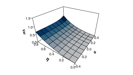
Figure 1: Asymptotic variance of $\hat{\eta}_{a}$, for $\eta\in(0,0.8]$, with $a\in[-0.4,\,0.4]$.

Theorem 3

Assume conditions of Theorem 1. Let $k=k(n)$ be an intermediate sequence such that $\sqrt{k}\,q_{\star}(n/k)\rightarrow 0$, as $n\rightarrow\infty$. Then, for every $a,b\in\real$, the estimator $\hat{\eta}_{a,b}^{(S)}(k)$ in the class (12), stemming from transformation to unit Fréchet marginals with a shift by $1/2$, is asymptotically equivalent to its standard counterpart $\hat{\eta}_{a,b}(k)$ in the class (8), i.e., as $n\rightarrow\infty$,

$$\sqrt{k}\,\bigl{|}\hat{\eta}_{a,b}^{(S)}(k)-\hat{\eta}_{a,b}(k)\bigr{|}\,\displaystyle{\mathop{\longrightarrow}^{P}}\,0.$$

Theorem 3 implies that, provided there is an appropriate upper bound on the intermediate sequence $k(n)$, the two classes of estimators ultimately (i.e., with probability tending to $1$, as $n\rightarrow\infty$) coincide in terms of their asymptotic distributions, with only possible remnant differences arising from the second order deterministic bias, which can nonetheless be made explicit in terms of $0<\eta\leq 1$ and $\rho>0$. In order to make matters simple, the present formulation for Theorem 3 assumes $\sqrt{k}\,q_{\star}(n/k)=o(1)$ which corresponds to imposing a further, yet mildly restrictive condition, upon the rate of growth of the intermediate sequence $k=k(n)$ in relation to the whole sample size $n$, meaning that differences in this second component of the bias are dominated by the main bias term $b_{a}(\eta,\tau)$ identified in Corollary 2.

4 Reduced bias estimation

Firstly, we present two basic definitions and a step anchoring theorem rooted in the theory of regular variation. At present the aim is to obtain a similar relation to (14) in terms of the quantile function associated with standardisation to unit Fréchet, defined as

$$V(t):=\Bigl{(}-\frac{1}{\log F}\Bigr{)}^{\leftarrow}(t)=U\Bigl{(}\frac{1}{1-e^{-1/t}}\Bigr{)},$$

with $U:=(1/(1-F))^{\leftarrow}$ and $F$ denoting the distribution function as usual. By writing concisely $V^{*}(t):=V(t)+1/2$, we get the formulation in the following theorem. The proof is deferred to Section 5.

Theorem 4

Let $U$ be a tail quantile function of regular variation at infinity with index $\eta\in(0,\,1]$, i.e. $\lim_{t\rightarrow\infty}U(tx)/U(t)=x^{\eta}$, for $x>0$, which we denote by $U\in RV_{\eta}$. Assume that the second order condition of regular variation (14) is satisfied for $U$ with second order parameter $\tau>0$. Then, $V^{*}$ is also regularly varying with the same index $\eta$ and is such that, for $x>0$,

$${\lim_{t\rightarrow{\infty}}}\frac{\frac{V^{*}(tx)}{V^{*}(t)}-x^{\eta}}{\tilde{q}(t)}=\left\{\begin{array}[]{ll}x^{\eta}\,\frac{x^{-\tau}-1}{\tau},&\,\tau<\eta,\\ x^{\eta}\,\frac{x^{-\eta}-1}{\eta},&\,\tau\geq\eta,\end{array}\right.$$ (16)

where

$$\tilde{q}(t)=\left\{\begin{array}[]{ll}{q}_{\star}(t),&\,\tau<\eta,\\ {q}_{\star}(t)+\frac{\eta}{2}\frac{1}{V^{*}(t)},&\,\tau=\eta,\\ \frac{\eta}{2}\frac{1}{V^{*}(t)},&\,\tau>\eta.\end{array}\right.$$

Moreover, $|\tilde{q}(t)|\in RV_{-\tilde{\tau}}$ with second order parameter governing the speed of convergence given by

$$\tilde{\tau}=\left\{\begin{array}[]{ll}{\tau},&\,0<\tau<\eta,\\ {\eta},&\,0<\eta\leq\tau.\end{array}\right.$$

The Hall-Welsh-type model (Hall and Welsh,, 1985), which is relevant to our aim of inference for the residual dependence index, arises as a consequence of Theorem 4. Namely, the interest is in those distribution functions whose extreme quantile-type function $V^{*}$ determines the following expansion as $t\rightarrow\infty$, $V^{*}(t)=C^{\eta}t^{\eta}(1+\eta D_{1}C^{-\tau}t^{-\tau}+\eta D_{2}C^{-\eta}t^{-\eta})$, for $C>0$, $D_{1}\in\real$ and $D_{2}\neq 0$, whereby $\tilde{q}(t)/\tilde{\tau}=\eta\tilde{\beta}t^{-\tilde{\tau}}$, with $\tilde{\beta}=D_{j}C^{-\tilde{\tau}}$ and $j=1$ if $\tilde{\tau}=\tau$, $j=2$ if $\tilde{\tau}=\eta$. Clearly, such a model for $V^{*}$ implies that the speed of convergence to the desired power function in the limit, describing the residual strength in the asymptotic independence attached to the index $\eta$, can be improved by means of the location-shift by $1/2$. In particular, the proof for Theorem 4, in Appendix B, emphasises that $V^{*}(tx)/V^{*}(t)-x^{\eta}$ has a similar representation to $U^{*}(tx)/U^{*}(t)-x^{\eta}$, here $U^{*}:=U+1/2$, as $t\rightarrow\infty$, but different to $V(tx)/V(t)-x^{\eta}$ by a term of third order kind.

The most straightforward, and perhaps even the most effective way of robbing estimator $\hat{\eta}^{(S)}_{a,b}$ of its second order bias, without disturbing the inherent asymptotic variance, is through coupling Corollary 2 with Theorem 3 whilst setting $b/a=-1$. This is indeed the gist to devising the new proposed reduced bias estimator. Let $V^{*}_{n,1}\leq V^{*}_{n,2}\leq\ldots\leq V^{*}_{n,n}$ be the ascending order statistics associated with the identically distributed random variables $V_{i}^{*(n)}:=V_{i}^{(n)}+1/2$, $i=1,2,\ldots,n$, with $V_{i}^{(n)}$ defined in (11). The reduced bias estimator thus arises as follows:

$$\widetilde{\eta}_{a}(k,k^{*}):=\hat{\eta}^{(S)}_{a,-a}(k)\biggl{\{}1-\biggl{(}\hat{\beta}\Bigl{(}\frac{n}{k}\Bigr{)}^{-\hat{\tau}}+\frac{1}{1+2V_{n,n-k^{*}}}\biggr{)}\frac{1-a\,\hat{\eta}^{(S)}_{a,-a}(k)}{1-a\,\hat{\eta}^{(S)}_{a,-a}(k)+\hat{\tau}}\biggr{\}},$$ (17)

with $k,k^{*}$, both intermediate sequences of positive integers, i.e., $k=k(n)\rightarrow\infty$, $k^{*}=k^{*}(n)\rightarrow\infty$, $k/n\rightarrow 0$, $k^{*}/n\rightarrow 0$ and such that $k^{*}/k\rightarrow 0$, as $n\rightarrow\infty$, and where $\hat{\beta}$ and $\hat{\tau}$ denote consistent estimators for $\overline{\beta}=\tilde{\tau}\tilde{\beta}$ (i.e., estimated at a stroke as a function of the two key parameters in the Hall-Welsh representation) and for $\tilde{\tau}>0$, respectively. Theorem (5) establishes large sample properties of the proposed reduced bias estimator of the residual dependence index $\eta$.

Theorem 5

Under conditions of Theorem 1, let $k^{*}$ and $k$ be two intermediate sequences of positive integers such that $k^{*}\leq\sqrt{k}$. Then,

1. the estimator $\widetilde{\eta}_{a}=\widetilde{\eta}_{a}(k,k^{*})$ as defined in (17) is a reduced-bias variant of the estimator $\hat{\eta}\equiv M_{a,-a}(Q_{n})$.

2. Moreover, if $k=k(n)$ satisfies $\sqrt{k}\,\tilde{q}(n/k)\rightarrow\lambda^{*}\in\real$, as $n\rightarrow\infty$, then

   $$\sqrt{k}\,\bigl{(}\widetilde{\eta}_{a}-\eta\bigr{)}\,\displaystyle{\mathop{\longrightarrow}^{d}}\,Z_{a},$$ (18)

   where $Z_{a}$ is a normal variable with mean zero and $\sigma_{a}^{2}>0$, the same asymptotic variance appearing in Corollary 2.

Remark 2

Given the conditions of Theorem 5, confidence bounds for the reduced bias estimator (17) of the residual dependence index $\eta$ follow readily from Corollary 2.

5 Proofs

The present section is comprised of all the proofs and auxiliary lemmas to the limit results in Sections 3 and 4.

5.1 Proofs for Section 3

Proof of Theorem 1: The starting point is the distributional representation for the quantile process in terms of standard uniform marginals. Under the second order condition (13) from Section 3, with $m:=nq(k/n)$ and $m\rightarrow\infty$, i.e., provided $k=k(n)\rightarrow\infty$, $k/n\rightarrow 0$, as $n\rightarrow\infty$, there exists a function $q_{\star}$ of constant sign near infinity and tending to zero, and whereby $\sqrt{m}\,q_{\star}(1/q^{\leftarrow}(m/n))=O(1)$, such that it is possible to define a sequence of standard Brownian motions $\{W_{n}(s)\}_{s\geq 0}$, in such a way that, for all $s_{0}>0$ and $\varepsilon>0$,

$$\sup_{0<s\leq s_{0}}s^{\eta+\frac{1}{2}+\epsilon}\left|\sqrt{m}\left(\frac{k}{n}Q_{n}(s)-s^{-\eta}\right)-\eta s^{-(\eta+1)}W_{n}(s)-\sqrt{m}\,q_{\star}\bigl{(}\frac{n}{k}\bigr{)}s^{-\eta}\frac{s^{\tau}-1}{\tau}\right|=o_{p}(1)$$ (19)

(cf. Goegebeur and Guillou,, 2012, Lemma 1 in the Appendix). We define, for $a\neq 0$,

$$Z_{n}(s):=\sqrt{m}\Big{\{}\Bigl{(}\frac{Q_{n}(s)}{Q_{n}(1)}\Bigr{)}^{a}-s^{-a\eta}\Bigr{\}},$$ (20)

as well as redefine the auxiliary function involved in the second order condition relating to $q_{\star}$ such that $q_{\star}(t)\sim q_{1}(1/t)$, as $t\rightarrow\infty$. By virtue of (19), we obtain

$$Z_{n}(s)=a\eta s^{-a\eta-1}\bigl{(}W_{n}(s)-sW_{n}(1)\bigr{)}+\sqrt{m}\,q_{\star}\Bigl{(}1/q^{\leftarrow}\bigl{(}\frac{m}{n}\bigr{)}\Bigr{)}s^{-a\eta}\frac{s^{\tau}-1}{\tau}+o_{p}\bigl{(}\max(s^{-\eta-1/2-\varepsilon},s^{-\eta})\bigr{)},$$

where the $o_{p}$-term is uniform on a compact interval bounded away from zero. After some algebra involving Taylor’s expansion around zero, we obtain the following asymptotic expansion with $\{B_{n}(s)\}\displaystyle{\mathop{=}^{d}}\{W_{n}(s)-sW_{n}(1)\}$, $s\in(0,\,1]$, a sequence of Brownian bridges:

$$\int_{0}^{1}Z_{n}(s)\,ds=a\eta\int_{0}^{1}s^{-a\eta-1}B_{n}(s)\,ds+\sqrt{m}\,q_{\star}\bigl{(}\frac{n}{m}\bigr{)}\int_{0}^{1}as^{-a\eta}\frac{s^{\tau}-1}{\tau}\,ds+o_{p}(1),$$ (21)

as $n\rightarrow\infty$. Since both $a,b$ are assumed fixed, the result in the theorem follows in a straightforward way via Cramèr’s delta-method for $a<1/(2\tau)$:

$$\sqrt{m}\biggl{\{}M_{a,b}(Q_{n})-\frac{(1-a\eta)^{-b/a}-1}{b}\biggr{\}}=\frac{1}{a}(1-a\eta)^{-b/a+1}\int_{0}^{1}Z_{n}(s)\,ds.$$

❏

Proof of Corollary 2: Theorem 1 ascertains that the random component $M_{a,b}(Q_{n})$, subtracted of deterministic bias, converges to an integral of a Brownian bridge (which is fundamentally a gaussian process). Given that increments of a gaussian process are independent normal random variables, this integral resolves to a sum of normals and hence a normal random variable in itself. If $\sqrt{m}\,q_{\star}(n/m)\rightarrow\lambda\in\real$, as $n\rightarrow\infty$, then the bias term in the limit results. Finally, in order to derive the variance of the limiting normal random variable, it suffices to consider the process $Z(s):=\eta s^{-a\eta-1}B(s)$, $0\leq s\leq 1$, for which $Var\bigl{(}\int_{0}^{1}Z(s)\,ds\bigr{)}=E\bigl{(}\int_{0}^{1}\int_{0}^{1}Z(s)Z(t)\,ds\,dt\bigr{)}=\eta^{2}\bigl{(}(1-a\eta)^{2}(1-2a\eta)\bigr{)}^{-1}$. ❏

Proof of Theorem 3: Consider the random pairs $(X_{i},Y_{i})$, $i=1,\ldots,n$, representing i.i.d. copies of $(X,Y)$. The primary focus is on the direct empirical analogue to the copula survival function $C(1-x,1-y)$ such that $C(x,y)=P\bigl{(}1-F_{1}(X)<x,1-F_{2}(Y)<y\bigr{)}$, which has at its core a summation of Bernoulli random variables associated with the non-independent, albeit identically distributed, $V_{i}^{(n)}$ (defined in (11) of Section 2). For an intermediate sequence $m=nq(k/n)$ and $m\rightarrow\infty$, we have for each $x\in[0,\,T]$, and $T>0$, $i=1,2,\ldots,n$, that by one hand,

$$\sum\limits_{i=1}^{n}\mathds{1}_{\{X_{i}\geq X_{n-[kx]+1,n},\,Y_{i}\geq Y_{n-[kx]+1,n}\}}$$ (22)

$$= \sum\limits_{i=1}^{n}\mathds{1}_{\bigl{\{}1-F_{1}^{(n)}(X_{i})\leq 1-F_{1}^{(n)}(X_{n-[kx]+1,n}),\,1-F_{2}^{(n)}(Y_{i})\leq 1-F_{2}^{(n)}(Y_{n-[kx]+1,n})\bigr{\}}}$$

$$= \sum\limits_{i=1}^{n}\mathds{1}_{\Bigl{\{}T_{i}^{(n)}\geq\frac{n}{[kx]}\bigr{)}\Bigr{\}}},$$

with $T_{i}^{(n)}$ from (7), of which the following properly standardised version satisfies, as $n\rightarrow\infty$,

$$\sqrt{m}\,\biggl{\{}\frac{\frac{1}{n}\sum\limits_{i=1}^{n}\mathds{1}_{\bigl{\{}\frac{k}{n}T_{i}^{(n)}\geq x\bigr{\}}}}{q(n/k)}-x^{-1/\eta}\biggr{\}}\,\displaystyle{\mathop{\longrightarrow}^{d}}\,W(x,x),$$

in $D([0,T])$, where $W$ is a zero-mean Gaussian process (cf. de Haan and Ferreira,, 2006, p. 268). On the other hand,

$$\sum\limits_{i=1}^{n}\mathds{1}_{\{X_{i}\geq X_{n-[kx]+1,n},\,Y_{i}\geq Y_{n-[kx]+1,n}\}} =\sum\limits_{i=1}^{n}\mathds{1}_{\bigl{\{}-\frac{1}{\log F_{1}^{(n)}(X_{i})}\geq-\frac{1}{F_{1}^{(n)}(X_{n-[kx]+1,n})},\,-\frac{1}{\log F_{2}^{(n)}(Y_{i})}\geq-\frac{1}{F_{2}^{(n)}(Y_{n-[kx]+1,n})}\bigr{\}}}$$

$$=\sum\limits_{i=1}^{n}\mathds{1}_{\Bigl{\{}\Bigl{(}-\frac{1}{\log F_{1}^{(n)}(X_{i})}\bigr{)}\wedge\bigl{(}-\frac{1}{\log F_{2}^{(n)}(Y_{i})}\bigr{)}\geq-\frac{1}{\log\bigl{(}1-\frac{[kx]}{n}\bigr{)}}\Bigr{)}\Bigr{\}}}$$

$$=\sum\limits_{i=1}^{n}\mathds{1}_{\Bigl{\{}V_{i}^{(n)}\geq-\frac{1}{\log\bigl{(}1-\frac{[kx]}{n}\bigr{)}}\Bigr{\}}}$$ (23)

with $V_{i}^{(n)}$ from (11) in Section 2. Owing to the power-series $\sum_{n\geq 0}\frac{t^{n}}{n+1}=-\frac{\log(1-t)}{t}$, for $|t|<1$, we can write the following stochastic inequalities for (23): there exists $\varepsilon>0$ such that

$$\mathds{1}_{\Bigl{\{}\frac{k}{n}\,V_{i}^{(n)}\geq\frac{1}{x}\Bigl{(}1-\frac{k}{n}\frac{x}{2}\bigl{(}1-\varepsilon(\frac{k}{n}x)^{\varepsilon}\bigr{)}\Bigr{)}\Bigr{\}}}\leq\mathds{1}_{\Bigl{\{}\frac{k}{n}\,V_{i}^{(n)}\geq-\frac{k/n}{\log\bigl{(}1-\frac{[kx]}{n}\bigr{)}}\Bigr{\}}}\leq\mathds{1}_{\Bigl{\{}\frac{k}{n}\,V_{i}^{(n)}\geq\frac{1}{x}\Bigl{(}1-\frac{k}{n}\frac{x}{2}\bigl{(}1+\varepsilon(\frac{k}{n}x)^{\varepsilon}\bigr{)}\Bigr{)}\Bigr{\}}},$$

uniformly in $x$ on a compact set bounded away from zero. This gives information about the error in the approximation of (23) to $\sum\limits_{i=1}^{n}\mathds{1}_{\Bigl{\{}\frac{k}{n}\bigl{(}V_{i}^{(n)}+\frac{1}{2})\geq\frac{1}{x}\Bigr{\}}}$. Specifically, for each $\delta>0$, there exists $\varepsilon^{\prime}>0$ chosen arbitrarily small, such that

$$\limsup_{n}\,P\Bigl{(}\max_{1\leq i\leq n}\bigl{|}I_{i}^{(n)}(x)-I_{i,\varepsilon^{\prime}}^{(n)}(x)\bigr{|}>1-\delta,\,\mbox{ for }0\leq x\leq T\Bigr{)}<\delta,$$

with intervening

$$I_{i}^{(n)}(x)=\mathds{1}_{\Bigl{\{}\frac{k}{n}\,V_{i}^{(n)}\geq-\frac{k/n}{\log\bigl{(}1-\frac{[kx]}{n}\bigr{)}}\Bigr{\}}}\quad\mbox{ and }\quad I_{i,\varepsilon^{\prime}}^{(n)}(x)=\mathds{1}_{\Bigl{\{}\frac{k}{n}\,V_{i}^{(n)}\geq\frac{1}{x}\Bigl{(}1-\frac{k}{n}\frac{x}{2}\bigl{(}1\pm\varepsilon^{\prime}(\frac{k}{n}x)^{\varepsilon^{\prime}}\bigr{)}\Bigr{)}\Bigr{\}}}.$$

The above inequalities thus imply, for each $n\in\mathbb{N}$, with $\delta,\,\varepsilon^{\prime}>0$ as before,

$$P\Bigl{(}\bigl{|}I_{i}^{(n)}(x)-I_{i,\varepsilon^{\prime}}^{(n)}(x)\bigr{|}\leq 1-\delta\,\mbox{ for all }i=1,\ldots,m;\,\mbox{ for }0\leq x\leq T\Bigr{)}>1-\delta.$$

By noting that

$$\frac{1}{n}\Bigl{|}\sum\limits_{i=1}^{n}\bigl{(}I_{i}^{(n)}(x)-I_{i,\varepsilon^{\prime}}^{(n)}(x)\bigr{)}\Bigr{|}\leq\frac{1}{n}\sum\limits_{i=1}^{n}\bigl{|}I_{i}^{(n)}(x)-I_{i,\varepsilon^{\prime}}^{(n)}(x)\bigr{|}\leq\max_{1\leq i\leq n}\bigl{|}I_{i}^{(n)}(x)-I_{i,\varepsilon^{\prime}}^{(n)}(x)\bigr{|},$$

and letting $\varepsilon^{\prime}>0$ be sufficiently close to zero, we arrive at

$$P\Bigl{(}\max_{1\leq i\leq n}\bigl{|}I_{i}^{(n)}(x)-I_{i,\varepsilon^{\prime}}^{(n)}(x)\bigr{|}=0\,\mbox{ for }\,0\leq x\leq T\Bigr{)}>1-\delta.$$

Now, invoking a Skorokhod construction, we have that, as $n\rightarrow\infty$, almost surely,

$$\sup_{x\in[0,T]}\,\Bigl{|}\frac{1}{n}\sum\limits_{i=1}^{n}\mathds{1}_{\Bigl{\{}V_{i}^{(n)}\geq-\frac{1}{\log\bigl{(}1-\frac{[kx]}{n}\bigr{)}}\Bigr{\}}}-\frac{1}{n}\sum\limits_{i=1}^{n}\mathds{1}_{\Bigl{\{}\frac{k}{n}\bigl{(}V_{i}^{(n)}+\frac{1}{2})\geq\frac{1}{x}\Bigr{\}}}\Bigr{|}\longrightarrow 0.$$ (24)

Together with (22), the above entails the asymptotic, almost sure, approximation of the suitably shifted Fréchet marginals to the standard Pareto marginals. This tells us that, for each $x$, the normalised sum $\frac{1}{n}\sum\limits_{i=1}^{n}\mathds{1}_{\bigl{\{}\frac{k}{n}\bigl{(}V_{i}^{(n)}+\frac{1}{2})\geq\frac{1}{x}\bigr{\}}}$ amounts to the rescaled empirical distribution function $1-F^{(n)}_{T}(x):=\frac{1}{n}\sum\limits_{i=1}^{n}\mathds{1}_{\bigl{\{}\frac{k}{n}T_{n,n-i}\geq x\bigr{\}}}$ and is such that $\bigl{(}1-F^{(n)}_{T}(x)\bigr{)}/q(k/n)=S(1/x,1/x)+O_{p}\bigl{(}1/\sqrt{nq(k/n)}\bigr{)}$. Then, a functional representation of the estimators considered on the basis of the tail empirical processes involved in (24) follows through the identification of the order statistics $V_{n,n-i}+1/2=T_{n,n-i}$ in relation to the standard Pareto marginals. Such an asymptotic representation is at the origin of the Hill estimator, in particular through the functional

$$\hat{\eta}^{H}\equiv M_{0}(k)=\frac{n}{m}\int_{T_{n,n-m}}^{\infty}\bigl{(}\log x-\log T_{n,n-m}\bigr{)}\,dF^{(n)}_{T}(x),$$

as well as to the general class of estimators

$$\hat{\eta}_{a,b}(k)=\frac{1}{b}\biggl{(}\Bigl{\{}\frac{n}{m}\int_{T_{n,n-k}}^{\infty}\bigl{(}\frac{x}{T_{n,n-k}}\bigr{)}^{a}\,dF^{(n)}_{T}(x)\Bigr{\}}^{b/a}-1\biggr{)}\,,$$

(see (8) and text around it, of which the Hill estimator is a member) and the result in the theorem thus follows. ❏

Remark 3

From the proof of Theorem 3 we find that the assertion involving $1-F^{(n)}_{T}(x):=\frac{1}{n}\sum_{i=1}^{n}\mathds{1}_{\bigl{\{}\frac{k}{n}T_{i}^{(n)}>x\bigr{\}}}$ is tantamount to establishing the approximation

$$\bigl{|}\frac{1}{n}\sum_{i=1}^{n}\mathds{1}_{\bigl{\{}\frac{k}{n}V_{i}^{(n)}>\frac{1}{x}\bigl{(}1-\frac{k}{n}\frac{x}{2}\bigr{)}\bigr{\}}}-\frac{1}{n}\sum_{i=1}^{n}\mathds{1}_{\bigl{\{}\frac{k}{n}\bigl{(}T_{i}^{(n)}-\frac{1}{2}\bigr{)}>\frac{1}{x}\bigl{(}1-\frac{k}{n}\frac{x}{2}\bigr{)}\bigr{\}}}\bigr{|}=o_{p}(1),$$

for $k\rightarrow\infty$, $k/n\rightarrow 0$, as $n\rightarrow\infty$. This is the change in location upon pseudo-observations for estimating the residual dependence index $\eta\in(0,\,1]$. In essence, it follows from Einmahl, (1997) and Peng, (1999) that

$$\sqrt{m}\,\Bigl{(}\frac{1}{m}\sum\limits_{i=1}^{n}\mathds{1}_{\bigl{\{}1-F_{1}(X_{i})\leq\frac{k}{n}x,1-F_{2}(Y_{i})\leq\frac{k}{n}x\bigr{\}}}-x^{-1/\eta}\Bigr{)}\,\displaystyle{\mathop{\longrightarrow}^{d}}\,W(x,x),$$

($W(x,x)\equiv W(x)$ is a zero-mean Gaussian process as before) and this corresponds to the properly reduced and standardised stochastic process

$$\sqrt{m}\,\biggl{(}\frac{\frac{1}{n}\sum\limits_{i=1}^{n}\mathds{1}_{\bigl{\{}T_{i}^{(n)}>\frac{n}{k}\frac{1}{x}\bigr{\}}}}{q(\frac{n}{k})}-x^{-1/\eta}\biggr{)}\,\displaystyle{\mathop{\longrightarrow}^{d}}\,W(x),$$

through the linkage $m/k:=(n/k)q(n/k)$, as $n\rightarrow\infty$. Upon this development, a suitable second order condition can be imposed which will determine an extra term in the approximation, akin to asymptotic bias. This condition of second order will then pin-down any potential changes in the second order parameter $\tau$ resulting from the shift by $1/2$. It also outlines the key idea to serve as the basis for Theorem 4.

5.2 Proofs for Section 4

Before getting underway with the proof of Theorem 4 we need a lemma, which mirrors the statement in Theorem 3, but now involving the extreme quantile functions $V:=\bigl{(}-1/\log{F}\bigr{)}^{\leftarrow}$ and $U:=\bigl{(}1/(1-t)\bigr{)}^{\leftarrow}$ which are associated with unit Fréchet and standard Pareto transforms, respectively.

Lemma 6

Define $V^{*}(t):=V(t)+1/2$. Suppose (14) holds for some $\eta\in(0,1]$ and $\tau>0$. Then,

$$\lim_{t\rightarrow\infty}\frac{U(t)}{V^{*}(t)}=1.$$

Proof: With the defined $V$ and $U$ it holds that $V(t)=U\bigl{(}\nicefrac{{1}}{{(1-e^{-1/t})}}\bigr{)}$, whence

$$\frac{U(t)}{V^{*}(t)}=\frac{U^{*}(t)}{U^{*}\Bigl{(}\frac{1}{1-e^{-1/t}}\Bigr{)}}-\frac{\nicefrac{{1}}{{2}}}{U^{*}\Bigl{(}\frac{1}{1-e^{-1/t}}\Bigr{)}},\qquad U^{*}:=U+\frac{1}{2},$$ (25)

with the latter term vanishing as $t\rightarrow\infty$. With $\widetilde{q}(t)=t^{-\eta}q_{\star}(t)U(t)$, $|\widetilde{q}(t)|\in RV_{-\tau}$, the second order regular variation for $U$ in (14) is written as

$${\lim_{t\rightarrow{\infty}}}\frac{(tx)^{-\eta}U(tx)-t^{-\eta}U(t)}{\widetilde{q}(t)}=\frac{x^{-\tau}-1}{\tau},$$ (26)

for all $x>0$. It implies in turn that with $U^{*}:=U+1/2$, as $t\rightarrow\infty$,

$$\frac{(tx)^{-\eta}U^{*}(tx)-t^{-\eta}U^{*}(t)}{\widetilde{q}(t)}=\frac{x^{-\tau}-1}{\tau}\bigl{(}1+o(1)\bigr{)}+\frac{x^{-\eta}-1}{2U(t)q_{\star}(t)},\qquad|U^{*}q_{\star}|\in RV_{-\tau+\eta},$$

i.e.,

$$x^{-\eta}\frac{U^{*}(tx)}{U^{*}(t)}-1=\Bigl{\{}\frac{x^{-\tau}-1}{\tau}\,q_{\star}(t)\frac{U(t)}{U^{*}(t)}+\frac{x^{-\eta}-1}{2}\frac{1}{U^{*}(t)}\Bigr{\}}\bigl{(}1+o(1)\bigr{)}$$ (27)

Additionally, we note that because $U\in RV_{\eta}$, $\eta>0$, we have for any constant $c\in\real$,

$$\frac{U(tx)-c}{U(t)-c}=\frac{U(tx)}{U(t)}\Bigl{(}1-\frac{c}{U(t)}\Bigr{)}^{-1}\bigl{(}1+o(1)\bigr{)}=\frac{U(tx)}{U(t)}\bigl{(}1+o(1)\bigr{)}.$$

Therefore, with $c=1/2$ in particular, we get that $U^{*}(t)\sim U(t)$, as $t\rightarrow\infty$, and also that by taking $y=U^{*}(tx)/U^{*}(t)$ in the equality $1/(1+y)=1-y+y^{2}/(1+y)$, $y\neq-1$, then relation (27) entails

$$x^{\eta}\frac{U^{*}(t)}{U^{*}(tx)}-1=-\frac{x^{-\eta}\frac{U^{*}(tx)}{U^{*}(t)}-1}{x^{-\eta}\frac{U^{*}(tx)}{U^{*}(t)}}=\frac{x^{-\tau}-1}{-\tau}q_{\star}(t)\bigl{(}1+o(1)\bigr{)}-\frac{x^{-\eta}-1}{2}\frac{1}{U^{*}(t)}\bigl{(}1+o(1)\bigr{)}.$$

Finally, Taylor’s expansion of $y/(1-e^{-y})$ around zero ascertains the result:

$$\frac{U^{*}(t)}{U^{*}\Bigl{(}\frac{1}{1-e^{-1/t}}\Bigr{)}}=\Bigl{(}\frac{\nicefrac{{1}}{{t}}}{1-e^{-1/t}}\Bigr{)}^{-\eta}=1-\frac{\eta}{2}\frac{1}{t}+\frac{\eta(1+3\eta)}{24}\frac{1}{t^{2}}+o\bigl{(}\max(q_{\star}(t),1/U^{*}(t))\bigr{)},$$

as $t\rightarrow\infty$, whereby we conclude that $U(t)\sim V^{*}(t)$ from the stated equality (25) at the beginning of this proof. ❏

Proof of Theorem 4: The proof essentially hinges on translating second order regular variation into extended regular variation of an appropriate function related to the former. With the already defined quantile function $V$, such that $V(t)=U\bigl{(}\nicefrac{{1}}{{(1-e^{-1/t})}}\bigr{)}$, and $\widetilde{q}(t)=t^{-\eta}q_{\star}(t)U(t)$, $|\widetilde{q}(t)|\in RV_{-\tau}$, we have that

$$\frac{(tx)^{-\eta}V(tx)-t^{-\eta}V(t)}{\widetilde{q}(t)} = \frac{(tx)^{-\eta}V(tx)-t^{-\eta}U(t)}{\widetilde{q}(t)}-\frac{t^{-\eta}V(t)-t^{-\eta}U(t)}{\widetilde{q}(t)}$$

$$= \frac{(tx)^{-\eta}U\bigl{(}\nicefrac{{1}}{{(1-e^{-1/(tx)})}}\bigr{)}-t^{-\eta}U(t)}{\widetilde{q}(t)}-\frac{t^{-\eta}U\bigl{(}\nicefrac{{1}}{{(1-e^{-1/t})}}\bigr{)}-t^{-\eta}U(t)}{\widetilde{q}(t)}.$$

Owing to the second order regular variation for $U$ with index $\eta>0$ encapsulated in (26), which holds locally uniformly for $x>0$, and by noting that $x(t)=\nicefrac{{t^{-1}}}{{(1-e^{-1/t})}}\rightarrow 1$, as $t\rightarrow\infty$, we find the representation:

$$\frac{(tx)^{-\eta}V(tx)-t^{-\eta}V(t)}{\widetilde{q}(t)}=\frac{\Bigl{(}\frac{1/t}{1-e^{-1/(tx)}}\Bigr{)}^{-\tau}-1}{\tau}\bigl{(}1+o(1)\bigr{)}-t^{-\eta}\frac{\Bigl{(}\frac{1/t}{1-e^{-1/t}}\Bigr{)}^{-\tau}-1}{\tau}\bigl{(}1+o(1)\bigr{)}.$$

Now it is only a matter of applying Taylor’s expansion followed by judicious manipulation in order to have, for all $x>0$, the next order representation:

$$\frac{x^{-\eta}\frac{V(tx)}{V(t)}-1}{q_{\star}(t)\,U(t)/V(t)}=\frac{x^{-\tau}-1}{\tau}-\frac{1}{2t}x^{-\tau-1}+o\bigl{(}\frac{1}{t}\bigr{)},$$ (28)

as $t\rightarrow\infty$. Moving on to tackling $V^{*}(t)=V(t)+1/2$, we consider the above development to approaching the extended regular variation property as follows:

$$\frac{(tx)^{-\eta}V^{*}(tx)-t^{-\eta}V^{*}(t)}{\widetilde{q}(t)} = \frac{(tx)^{-\eta}V(tx)-t^{-\eta}V(t)}{\widetilde{q}(t)}+\frac{t^{-\eta}}{2}\frac{x^{-\eta}-1}{\widetilde{q}(t)}$$

$$= \frac{x^{-\tau}-1}{\tau}+\frac{t^{-\eta}}{\widetilde{q}(t)}\frac{x^{-\eta}-1}{2}-\frac{1}{t}\frac{x^{-\tau-1}}{2}+o(t^{-1})+o(1).$$

Given that the present setting of asymptotic independence the range $\eta\leq 1$ is to be imposed, the third order term in (28) becomes negligible (note that $|t^{\eta}\widetilde{q}(t)|\in RV_{-\tau+\eta}$ and $\eta<1+\tau$, $\tau>0$), thus resulting in the following representation for $V^{*}$:

$$\frac{x^{-\eta}\frac{V^{*}(tx)}{V^{*}(t)}-1}{q_{\star}(t)\,U(t)/V^{*}(t)}=\frac{x^{-\tau}-1}{\tau}+\frac{1}{q_{\star}(t)U(t)}\frac{x^{-\eta}-1}{2}+o\Bigl{(}\frac{1}{q_{\star}(t)U(t)}\Bigr{)}.$$

Under the conditions of this theorem, Lemma 6 above now enables replacement of $U$ with $V^{*}$ everywhere in the expansion above and the desired result of second order regular variation for $V^{*}$ arises. Specifically,

$$\frac{V^{*}(tx)}{V^{*}(t)}=q_{\star}(t)\,x^{\eta}\frac{x^{-\tau}-1}{\tau}+\frac{\eta}{2}\frac{1}{V^{*}(t)}\,x^{\eta}\frac{x^{-\eta}-1}{\eta}+o\bigl{(}q_{\star}(t)\bigr{)}+o\Bigl{(}\frac{1}{V^{*}(t)}\Bigr{)}\qquad(t\rightarrow\infty).$$

❏

Proof of Theorem 5: The first part of the theorem is ensured by Theorem 3 in conjunction with Theorem 4. In particular, note that (14) implies (16) through suitable adaptation in relation to the auxiliary function of second order. For the second part, we write:

$$\sqrt{k}\left(\widetilde{\eta}_{a}(k)-\eta\right)=\sqrt{k}\,\biggl{\{}\hat{\eta}^{(S)}_{a}(k)\biggl{(}1-\hat{\beta}\Bigl{(}\frac{n}{k}\Bigr{)}^{-\hat{\tau}}\frac{1-a\,\hat{\eta}^{(S)}_{a}(k)}{1-a\,\hat{\eta}^{(S)}_{a}(k)+\hat{\tau}}\biggr{)}-\eta\biggr{\}}+\sqrt{k}\,\frac{\hat{\eta}^{(S)}_{a}(k)}{2}\frac{1}{V^{*}_{n,n-k^{*}}}\frac{1-a\,\hat{\eta}^{(S)}_{a}(k)}{1-a\,\hat{\eta}^{(S)}_{a}(k)+\hat{\tau}}.$$ (29)

The methodology in Caeiro et al., (2005) ascertains that the remnant bias in the first $\sqrt{k}$-term is of lower order than that associated with the relevant assumption $\sqrt{k}\,\tilde{q}(n/k)=O(1)$, as $n\rightarrow\infty$, with ensuing asymptotic expansion

$$\sqrt{k}\,\biggl{\{}\hat{\eta}^{(S)}_{a}(k)\biggl{(}1-\hat{\beta}\Bigl{(}\frac{n}{k}\Bigr{)}^{-\hat{\tau}}\frac{1-a\,\hat{\eta}^{(S)}_{a}(k)}{1-a\,\hat{\eta}^{(S)}_{a}(k)+\hat{\tau}}\biggr{)}-\eta\biggr{\}}=Z_{a}+o_{p}\bigl{(}\sqrt{k}\,\tilde{q}(n/k)\bigr{)},$$ (30)

where $Z_{a}$ is a Normal random variable with mean zero and variance $\sigma_{a}^{2}>0$ from Corollary 2. It remains to prove that the last term in (29) becomes negligible with $k^{*}\leq k$ for sufficiently large $n$. To this end, we find that

$$0<\frac{\sqrt{k}\,k^{*}/n}{\bigl{(}\frac{k^{*}}{n}V^{*}_{n,n-k^{*}}-1\bigr{)}+1}=\sqrt{k}\,\frac{k^{*}}{n}\Biggl{\{}1-\Bigl{(}\frac{k^{*}}{n}V^{*}_{n,n-k^{*}}-1\Bigr{)}+\frac{\Bigl{(}\frac{k^{*}}{n}V^{*}_{n,n-k^{*}}-1\Bigr{)}^{2}}{\frac{k^{*}}{n}V^{*}_{n,n-k^{*}}}\Biggr{\}}\leq\frac{k}{n}\biggl{\{}1+O_{p}\Bigl{(}\frac{1}{\sqrt{k}}\Bigr{)}+o_{p}\Bigl{(}\frac{1}{\sqrt{k}}\Bigr{)}\biggr{\}}.$$

The last inequality is ensured by $k^{*}\leq k$ and Lemma 1 in Appendix B coupled with Lemma 2.2.3 of de Haan and Ferreira, (2006). ❏

6 Simulation results

The simulation results this section encompasses draw on $N=1000$ i.i.d. copies (or replicates) of the random sample $(X_{i},Y_{i})$, $i=1,\ldots,n$, from the continuous distribution function $F$ on ² with univariate marginal distributions $F_{j}$, $j=1,2$, and whose dependence structure is uniquely determined by the copula function $C:[0,1]^{2}\rightarrow[0,1]$, such that $C(u,v)=F\bigl{(}F_{1}^{\leftarrow}(u),\,F_{2}^{\leftarrow}(v)\bigr{)}$, $0<u,v<1$ (Sklar,, 1959). Since we are interested in assessing dependence at large values, it is only natural to consider the corresponding survival copula $C^{s}(u,v)=u+v-1+C(1-u,1-v)$ for characterising domains of attraction as featured in condition (5). The paper by Goegebeur and Guillou, (2012) offers a good catalogue of copulas belonging to the domain of attraction of a bivariate extreme value distribution, falling in the case of asymptotic independence, meaning that (residual) dependence is present until the actual extreme value limit is reached. The two copulas addressed below also satisfy condition (14) for some $\eta\in(0,1)$ and $\tau>0$. Specifically:

1. Frank distribution with copula function

   $$\mathcal{C}_{\theta}(u,v)=-\frac{1}{\theta}\log\Bigl{(}1-\frac{(1-e^{-\theta u})(1-e^{-\theta v})}{1-e^{-\theta}}\Bigr{)},\quad(u,v)\in[0,1]^{2},\;\theta>0,$$

   satisfying the second order condition (14) with $\eta=\tau=1/2$.

2. Ali-Mikhail-Had distribution, whose copula function is given by

   $$\mathcal{C}_{\theta}(u,v)=\frac{u\,v}{1-\theta(1-u)(1-v)},\quad(u,v)\in[0,1]^{2},\;\theta\in[-1,1].$$

   For $\theta=-1$ the second order condition (14) holds with $\eta=1/3$ and $\tau=2\eta=2/3$.

These were selected not only for their flexibility in terms of the association being induced into the random pair $(X,Y)$, but also because they have been found to mirror the asymptotically independent rainfall data analysed as part of the application of the proposed estimators in a satisfactory way. We have conducted a much wider simulation study, with many more distributions under scrutiny, for several sample sizes. A considerable number of these are presented in Appendices A and B. It was mainly in the light of that comprehensive numerical study that we have settled with performance evaluation of the new class of estimators for the residual dependence index by drawing on $N=1000$ replicates of the random sample consisting of $n=500$ pairs $(X_{i},Y_{i})$, $i=1,2,\ldots,n$. The residual dependence index $\eta\in(0,1]$ was estimated by $\hat{\eta}^{(S)}_{q}\equiv\hat{\eta}^{(S)}_{1/p,1/q-1}$, $1/p+1/q=1$, and subsequently through the reduced bias estimator $\widetilde{\eta}_{q}$ defined in (17).

Although the two parameters $\eta$ and $\tau$ are viewed as the main design factor in the finite sample numerical experiments, there is another related quantity which needs addressing when it comes to the new proposed class of estimators for $\eta$. The distortion parameter $a\in\real$ plays a significant part in the proposed estimation. Notably, its natural range (on the positive reals) breaks down into two regions that come out well aligned with the direction of association in the random pair $(X,Y)$. The benchmark value $\eta=1/2$ sets the case of nearly independent components $X$ and $Y$. In this case, the requirement for finite asymptotic variance, in that $1/q>1-1/(2\eta)$ (cf. Corollary 2), is of little consequence as it implies that $q$ must be some positive value. If $\eta>1/2$, meaning that realisations of $(X,Y)$ exceeding the same high threshold are more frequent than they would under exact independence, then the finite variance constraint will impose an upper bound for $q$. Finally, if $0<\eta<1/2$, where exceedances of the same threshold occur less frequently than in case of complete independence, that requirement translates into a lower bound for $q$. This lower bound can be negative and therefore does not curtail the basic assumption of $q>0$. Additionally, in terms of asymptotic bias, setting $b/a=-1$ in (12) (i.e. the Fréchet-margins asymptotic equivalent to (10)) ascertains the dominant component of the asymptotic bias is always positive and at most $1$. We recall that the second order bias for the Hill estimator is $1/(1+\tau)$, here attained as $q$ approaches $1$. For the second order bias to be less than or equal to zero, one would need $a=1-1/q\geq 1/\eta$, which is an impossibility given the primary restriction that $a<1/(2\eta)$. Therefore, overall the proposed class of estimators (12) stand to gain improved performance for a residual dependence index close to zero. On the other hand, choosing a distortion value $q$ close to zero (i.e. $a\rightarrow-\infty$) leads to approximately constant bias (i.e. approaching $1$), thus breaking the inherent link of the latter to both $\eta$ and $\tau$.

Figures 2 and 3 display estimated bias and mean squared error resulting from the $N=1000$ estimates by adopting $\hat{\eta}_{q}^{(S)}$, and related reduced bias versions $\widetilde{\eta}^{(S)}_{q}$ with varying $q=0.1(0.1)1.9$, into the estimation of $\eta$ for each of the prescribed copulas (i) and (ii). The key findings determined by the simulation study, which Figures 2 and 3 represent, are outlined as follows:

• Specifying a value of $q$ away from $1$ generally worsens the bias but does not seem to affect the estimated variance much. If the true value of $\eta$ in the close vicinity of $1/2$, i.e., in the near independence setting, estimators $\hat{\eta}_{q}^{(S)}$ seem to gain improved finite-sample performance through the specification of a value $q$ slightly above $1$.

• Only a small top sample fraction $k/n$, accounting for up to $k/n=0.1$, is advisable in the estimation of $\eta$ by adopting $\widetilde{\eta}^{(S)}_{q}$. Since the asymptotic bias is always positive, one must leverage on the variance in order to maximise finite sample performance of this proposed estimator and stay clear of large $k$ where bias usually sets in. The simulation results in Appendix A strongly corroborate this finding.

• Reduced bias estimators $\widetilde{\eta}^{(S)}_{q}$ attached to $q<1$ exhibit the best finite sample behaviour. Values of $q$ slightly below $1$ seem to be generally preferable because the resulting bias is more likely to come out unaffected by any potentially slow convergence to the relevant bivariate extreme value distribution (i.e. for small values of $\tau>0$). With fewer contributing factors, the asymptotic bias is poised to be more effectively removed. To this end, the number $k^{*}$ of upper pseudo-observations of the type (11) does not seem to play a crucial role, as long as it stays less than or equal to $\sqrt{k}$. A fractional power of $n$ such as $k^{*}=[n^{0.3}]$, whilst keeping $k^{*}$ sufficiently large, has also been deemed adequate in light of our numerical experiments.

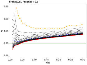
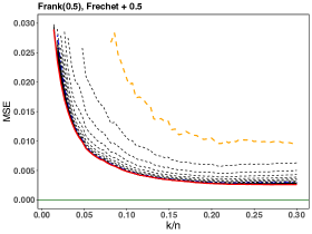
(a)	(b)
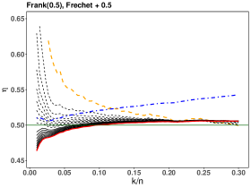
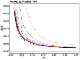
(c)	(d)
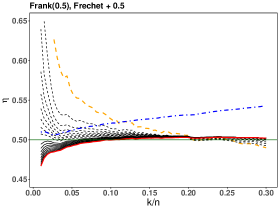
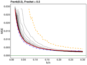
(e)	(f)

Figure 2: Frank copula with $\theta=0.5$ ($\eta=\tau=1/2$): (a) and (b) result from $\hat{\eta}^{(S)}_{q}(k)$; (c) and (d) correspond to the reduced bias version $\widetilde{\eta}^{(S)}_{q}(k)$, $k^{*}=[n^{0.3}]$, whereas (e) and (f) use $k^{*}=[\sqrt{k}]$. Dashed lines identify $q<1$ with orange line for the lower bound $q=0.1$; solid lines render $q>1$ with red highlighting the upper bound $q=1.9$. The blue dash-dotted line depicts the Hill estimator.

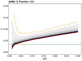
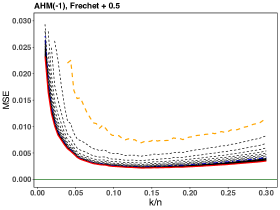
(a)	(b)
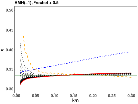
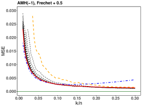
(c)	(d)
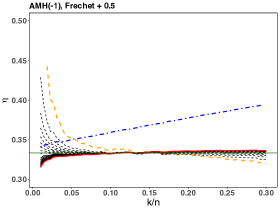
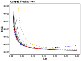
(e)	(f)

Figure 3: Ali-Mikhail-Haq copula with $\theta=-1$ ($\eta=1/3,\tau=2/3$): (a) and (b) result from $\hat{\eta}^{(S)}_{q}(k)$; (c) and (d) correspond to the reduced bias version $\widetilde{\eta}^{(S)}_{q}(k)$, $k^{*}=[n^{0.3}]$, whereas (e) and (f) use $k^{*}=[\sqrt{k}]$. Dashed lines identify $q<1$ with orange line for the lower bound $q=0.1$; solid lines render $q>1$ with red highlighting the upper bound $q=1.9$. The blue dash-dotted line depicts the Hill estimator.

7 Residual dependence in tropical extreme rainfall

The new class of estimators for the residual dependence index $\eta>0$ introduced in this paper is now applied to the study of extreme values arising in tropical rainfall observations recorded both at nearby gauging stations (i.e. within the range 5-15$km$) and pairs of stations as far apart as 190-200$km$. To this end, we looked at daily rainfall measurements collected over 68 years, comprising the period between the years 1950 and 2017, at 591 irregularly spaced stations across Ghana. Ghana has a strong seasonal rainfall cycle regulated by the West African monsoon, so the present analysis will focus on daily rainfall measurements collected every June pertaining to 68 years worth of available data, thus targeting the peak of the main rainy season, with the obvious advantage that it contains the largest proportion of rainy days and the greatest number of extreme rainfall occurrences.

To ensure that the data is identically distributed, we will only consider the stations in the southern part of the country. None of the individual time series are without missing values, and the proportion of these are ranging between 5%-95%. As an initial screening, we remove all stations with more than 3000 missing values, equalling about 12% of the full time series, which leaves us with 40 stations to select pairs from. To minimise distributional variations due to systematic features in the spatial domain, one of the three chosen stations (ASU) is common for the two pairs and the two pairs are roughly aligned on the same bearing. Figure 4 highlights this with BRI located 5-10$km$ away from ASU, and MAM 190-200$km$ away. After pre-processing the data recorded at each station, in order to remove inconsistencies, we were left with 1830 bivariate observations validated for our analysis of whether asymptotic independence is present for extreme values in the data. In Israelsson et al., (2020), it is concluded that for moderate values of rainfall, stations located more than 150$km$ apart appear to no longer exhibit dependence in terms of simultaneous rainfall occurrences. However, some evidence was found of tenuous dependence in very heavy rainfall (i.e. of magnitude $>50mm$), during the month of June, even for pairs of stations at such long distance as $150km$ apart. Building on these findings, we have settled with 190-200$km$ as a benchmark for the distance at which we expect to find some evidence of asymptotic independence in extreme tropical rainfall.

In the setting of this application to estimating residual dependence in very heavy rainfall, $n$ denotes the number of days with positive rainfall. Importantly, since even during the monsoon season there are many dry days (i.e., daily rainfall amounts $<1mm$), we have chosen to conduct estimation of the residual dependence index by drawing only on rainy days with rainfall measurements above the 90%-empirical quantile.

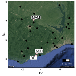
Figure 4: Map over southern Ghana highlighting the selected stations.

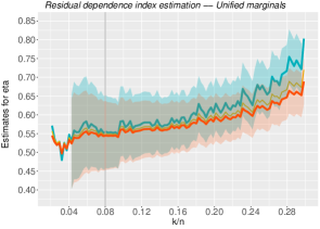
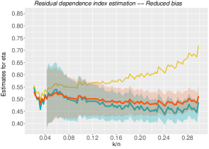
(a)	(b)
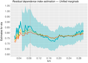
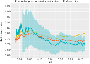
(c)	(d)

Figure 5: Estimation of the residual dependence index using $q=0.5,1.5$ in $\hat{\eta}^{(S)}_{q}$ and associated reduced bias variant: plots (a)-(b) correspond to the long range residual dependence analysis in the study. The blue thick line gives the sample path for $q=0.5$, whereas the red solid line corresponds to the $q=1.5$. Shaded areas indicate their respective $95\%$ confidence bands. The yellow line depicts the Hill estimator; plots (c)-(d) are the similar plots for the nearby stations.

Figure 5 shows the sample paths yielded by three members of the new class of estimators (12) through the parametrisation $(a,b)=(1/p,1/q-1)$, $1/p+1/q=1$, including the Hill estimator. All three estimators $\hat{\eta}^{(S)}_{q}$, $q=0.5,1,1.5$ seem to deliver a plateau of stability around $k/n=8\%$ for both pairs of considered in this analysis. For the stations further apart, in particular, the $\eta$-estimates displayed in plot (a) show an appreciable stability region for $k/n=6\%$ up to $k/n=10\%$, approximately, with the resulting $\eta$-estimates tending to hover about $0.55$. Then, plot (b) adds to the stability region in the sense that the reduced bias estimates stemming from the two estimators $\widetilde{\eta}_{0.5}(k)$ and $\widetilde{\eta}_{1.5}(k)$ (both members of the class (17)) enhance consistency in the estimation for a wide range of $k/n$. Noticeably, estimator $\widetilde{\eta}_{1.5}$ enables to settle with the overall estimate for the residual tail index of $\hat{\eta}=1/2$. This means that it is reasonable to the conclude that the near independence regime is plausible for very large rainfall amounts emanating from stations ASU and MAM. This conclusion conforms to the preliminary findings upon Figure 6 (b), where the points seem to be evenly distributed over the unit square, with no particular pattern standing out.

Similarly as before, plot (d) on the right hand-side of Figure 5 displays the sample paths yielded by two reduced bias estimators, both $\widetilde{\eta}_{0.5}(k)$ and $\widetilde{\eta}_{1.5}(k)$, again alongside their primary estimators $\hat{\eta}^{(S)}_{q}$, $q=0.5,1,1.5$ bearing on the unifying marginal transform shown in plot (c). Just like their underpinning estimators $\hat{\eta}^{(S)}_{q}$, these reduced bias variants have been devised in such a way as to hold the advantage of putting aside any considerations on the practicalities of choosing standard Pareto over unit Fréchet marginal transformation (or vice-versa) that would normally take place before moving on to the actual statistical modelling of extreme residual dependence.

The difference between the plots (c) and (d) of $\eta$-estimates and the analogous plots (a) and (b) for the pair (ASU,MAM), with station MAM at a much longer distance from ASU than that for station BRI, is rather striking. Informed by the simulation results in Section 6 in conjunction with Figure 6 (a), we favour a value $q$ less than 1 in the enssuing estimation of the residual tail index $\eta$. This is mainly due to the likely presence of an $\eta>1/2$. Indeed, Figure 6 (a) suggests a positive association in the larger daily rainfall values for the nearby stations ASU and BRI as the data points seem to cluster in the right upper corner of this plot. Proceeding with the actual estimation, we find that there is little difference between sample paths from the canonical estimation by $\hat{\eta}^{(S)}_{0.5}(k)$ and those obtained through its reduced bias variant $\widetilde{\eta}_{0.5}(k)$, a remark that also holds true for the other distorted estimator in this analysis, $\widetilde{\eta}_{1.5}(k)$. This feature does not necessarily constitute a disadvantage but rather it indicates that the underpinning bivariate distribution has a fast convergence rate to the appropriate limiting extreme value distribution. By comparing the two plots (c)-(d) with one another, it is possible to update the point estimate sitting on $k/n=0.085$ to the one determined by the higher fraction $k/n=0.12$, thus averting wasteful use of information and giving rise to the overall $\hat{\eta}=0.765$. To not observe complete dependence associated with $\eta=1$, even at such a short distance, is to be expected for tropical rainfall, where sporadic but intense storms tend affect only a small area of a few square-kilometres. Additionally, in the situation where a convective storm is initiated over one station and travels in the opposite direction to the paired station, only one of them will record rainfall, hence reducing the dependence between them.

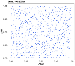
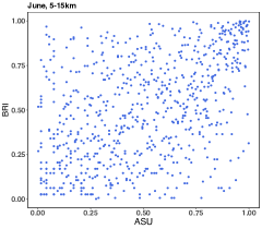
(a)	(b)

Figure 6: Scatter plots of positive rainfall values, transformed to the unit uniform scale, collected at two pairs of stations: (a) (ASU, MAM) and (b) (ASU, BRI).

As a final note, we mention that the second order parameters $\beta$ and $\tau$ have been estimated externally using the methodology in Caeiro et al., (2005, software available at: http://merlot.stat.uconn.edu/~jyan/docs/evrisk_r/CaeiroGomes/) and then plugged in to the estimators $\widetilde{\eta}_{q}(k)$, $q=0.5,1.5$, featuring in this applied study. In particular, we have followed the guidelines in Caeiro et al., (2005) which advise that, for a sample of size $n$, all second order parameters must be estimated at the considerably lower (random) threshold ascribed to $k=[n^{0.999}]$, where $[a]$ denotes the largest integer small than or equal to $a\in\real$.

Supplementary Material

The supplement related to this article is available online at: https://bit.ly/3izcI83. The supplementary material consists of one supporting information document containing further performance assessment, via numerical simulations, of the proposed class of estimators for the residual dependence index by drawing on four families of survival copulas, irrespective of marginals transformation. The primary performance measure adopted to this endeavour is the estimated mean squared error.

ORCID

Jennifer Israelsson https://orcid.org/0000-0001-6181-1702

Emily Black https://orcid.org/0000-0003-1344-6186

Cláudia Neves https://orcid.org/0000-0003-1201-5720

David Walshaw https://orcid.org/0000-0002-5267-2437

Appendix A Simulation results

In the interest of completeness, this section is devoted to presenting simulation results on the basis of four copula families outlined below.

1. Farlie-Gumbel-Morgenstern: $\mathcal{C}_{\theta}(u,v)=uv\{1+\theta(1-u)(1-v)\}$, $(u,v)\in[0,1]^{2},\,\theta\in[-1,1]$. Hence, with $\theta>-1$,

   $$\frac{P(1-F_{1}(X)<tx,1-F_{2}(Y)<ty)}{P(1-F_{1}(X)<t,1-F_{2}(Y)<t)}=xy\Bigl{\{}1-\frac{\theta t}{1+\theta}(x+y-2)+O(t^{2})\Bigr{\}},$$

   as $t\rightarrow\infty$, yields $\eta=\tau=1/2$ in (14).

2. Frank distribution with copula function

   $$\mathcal{C}_{\theta}(u,v)=-\frac{1}{\theta}\log\Bigl{(}1-\frac{(1-e^{-\theta u})(1-e^{-\theta v})}{1-e^{-\theta}}\Bigr{)},\quad(u,v)\in[0,1]^{2},\;\theta>0,$$

   satisfying the second order condition (14) with $\eta=\tau=1/2$.

3. Ali-Mikhail-Had distribution, whose copula function is given by

   $$\mathcal{C}_{\theta}(u,v)=\frac{u\,v}{1-\theta(1-u)(1-v)},\,(u,v)\in[0,1]^{2},\;\theta\in[-1,1].$$

   For $\theta=-1$ the second order condition (14) is satisfied with $\eta=1/3$ and $\tau=2\eta=2/3$.

4. Bivariate Normal: $\mathcal{C}_{\theta}(u,v)=\Phi_{\theta}\bigl{(}\phi^{-1}(u),\phi^{-1}(v)\bigr{)}$ with $\Phi_{\theta}$ the bivariate standard normal distribution function with correlation $\theta\in[-1,1]$ and $\Phi$ the scalar standard normal distribution function. Although the bivariate normal distribution with $\theta<1$ satisfies (13) with $\eta=\frac{1+\theta}{2}$, the resutling $\tau=0$ deems it out of scope in to relation the setting laid by (14) for this paper. Nonetheless, we choose to include it for assessing robustness.

Figures 7 to 10 display finite sample behaviour of estimators $\hat{\eta}_{q}$, introduced in (10), and the new class of estimators $\hat{\eta}_{q}^{(S)}$ given by (12) with $(a,b)=(1/p,1/q-1)$ in the following way. Performance assessment of the estimators is based on the estimated mean (on the left hand-side) of each Figure 7 to 10, and estimated mean squared error (MSE) (on the right hand-side), as a function of the top sample fraction $k/n\leq 0.3$. The parameter $q$ takes values $0.1(0.1)1.9$. The Hill estimator is retrieved for $q=1$. The aim of this section is to bear out the asymptotic equivalence established in Theorem 3 through finite sample behaviour of the relevant estimators by drawing on the four copula models above. All Figures conform to that transformation to Pareto or Fréchet with the shift by $1/2$ determines virtually the same findings for this class of estimators for the residual dependence index $\eta\in[0,1)$. There are instances at which the shifted Fréchet transformation leads to marginal improvement, for example in case of the underlying Farlie-Gumbel-Morgenstern copula, but this is not always the case. Taking everything into account, it seems reasonable to conclude that this choice of marginals does not play a role eventually, for the general class of estimators (8). Moreover, a selection of $q<1$ should take preference if there is preliminary evidence that the true value $\eta$ is greater than $1/2$, whereas a value $q>1$ should be specified in connection with potential $\eta<1/2$. The intermediate case of near independence $\eta=1/2$ is quite mixed, but it is also in this case that the reduced bias estimators seem to have best performance, thus making a choice of $q$ less relevant.

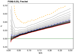
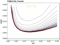
(a)	(b)
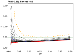
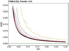
(c)	(d)
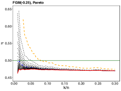
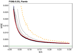
(e)	(f)

Figure 7: Farlie-Gumbel-Morgenstern copula with $\theta=-0.25$ ($\eta=\tau=1/2$). Plots (a) and (b) stem from unit Fréchet marginals; (c) and (d) result from adding the location shift; plots (e) and (f) correspond to the typical standard Pareto marginals. Dashed lines identify $q<1$ with orange for $q=0.1$, solid lines represent $q>1$ with red for $q=1.9$. The blue dash-dotted line in between ($q=1$) corresponds to the Hill estimator.

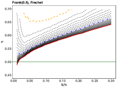
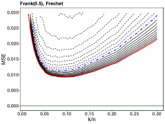
(a)	(b)
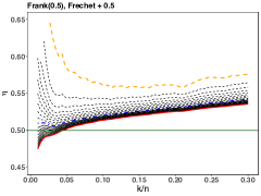
(c)	(d)
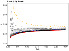
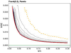
(e)	(f)

Figure 8: Frank copula with $\theta=0.5$ ($\eta=\tau=1/2$). Plots (a) and (b) stem from unit Fréchet marginals; (c) and (d) result from adding the location shift; plots (e) and (f) correspond to the typical standard Pareto marginals. Dashed lines identify $q<1$ with orange for $q=0.1$, solid lines represent $q>1$ with red for $q=1.9$. The blue dash-dotted line in between ($q=1$) corresponds to the Hill estimator.

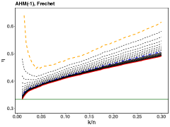
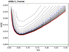
(a)	(b)
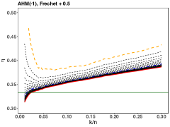
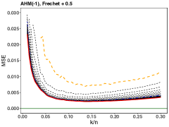
(c)	(d)
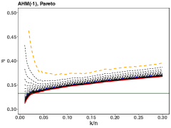
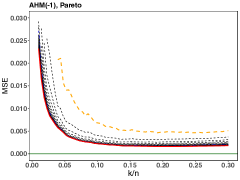
(e)	(f)

Figure 9: Ali-Mikhail-Haq copula with $\theta=-1$ ($\eta=1/3$, $\tau=2/3$). Plots (a) and (b) stem from unit Fréchet marginals; (c) and (d) result from adding the location shift; plots (e) and (f) correspond to the typical standard Pareto marginals. Dashed lines identify $q<1$ with orange for $q=0.1$, solid lines represent $q>1$ with red for $q=1.9$. The blue dash-dotted line in between ($q=1$) corresponds to the Hill estimator.

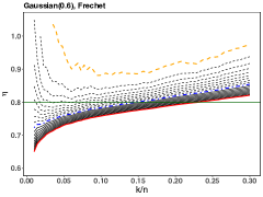
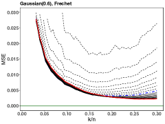
(a)	(b)
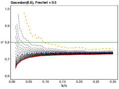
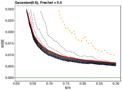
(c)	(d)
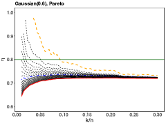
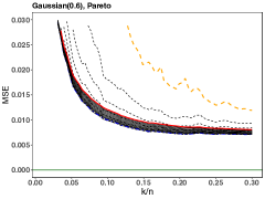
(e)	(f)

Figure 10: Gaussian copula with $\theta=0.6$ ($\eta=0.8,\tau=0$). Plots (a) and (b) stem from unit Fréchet marginals; (c) and (d) result from adding the location shift; plots (e) and (f) correspond to the typical standard Pareto marginals. Dashed lines identify $q<1$ with orange for $q=0.1$, solid lines represent $q>1$ with red for $q=1.9$. The blue dash-dotted line in between ($q=1$) corresponds to the Hill estimator.

Appendix B Further simulation results

The following results correspond to the mean-of-order $p$ class of estimators, corresponding to the parametrisation $(a,b)=(1/(1-p),\,q-1)$ with $1/p+1/q=1$ in both (10) and (12). This section aims to demonstrate that the simulation results are more discrepant and less consistent than those stemming from the leading parametrisation $(a,b)=(p^{-1},\,q^{-1}-1)$, in the sense that values of $q$ well above 1 or much lower than 1 are often required in order to minimise bias, and thereby attaining optimal mean squared error.

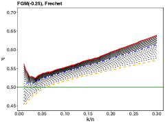
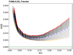
(a)	(b)
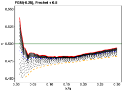
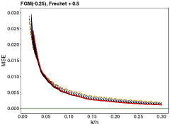
(c)	(d)
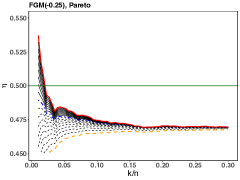
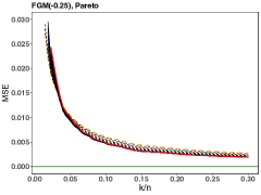
(e)	(f)

Figure 11: Farlie-Gumbel-Morgenstern copula with $\theta=-0.25$ ($\eta=\tau=1/2$). Plots (a) and (b) stem from unit Fréchet marginals; (c) and (d) result from adding the location shift; plots (e) and (f) correspond to the typical standard Pareto marginals. Dashed lines identify $q<1$ with orange for $q=0.1$, solid lines represent $q>1$ with red for $q=1.9$. The blue dash-dotted line in between ($q=1$) corresponds to the Hill estimator.

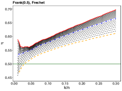
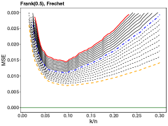
(a)	(b)
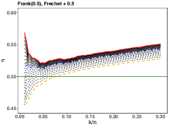
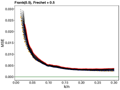
(c)	(d)
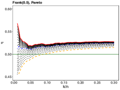
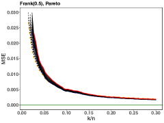
(e)	(f)

Figure 12: Frank copula with $\theta=0.5$ ($\eta=\tau=1/2$). Plots (a) and (b) stem from unit Fréchet marginals; (c) and (d) result from adding the location shift; plots (e) and (f) correspond to the typical standard Pareto marginals. Dashed lines identify $q<1$ with orange for $q=0.1$, solid lines represent $q>1$ with red for $q=1.9$. The blue dash-dotted line in between ($q=1$) corresponds to the Hill estimator.

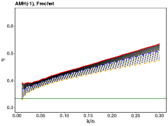
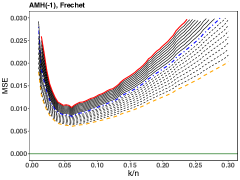
(a)	(b)
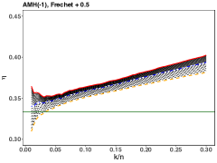
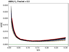
(c)	(d)
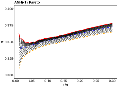
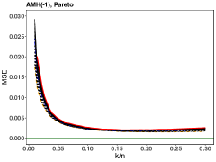
(e)	(f)

Figure 13: Ali-Mikhail-Haq copula with $\theta=-1$ ($\eta=1/3$, $\tau=2/3$). Plots (a) and (b) stem from unit Fréchet marginals; (c) and (d) result from adding the location shift; plots (e) and (f) correspond to the typical standard Pareto marginals. Dashed lines identify $q<1$ with orange for $q=0.1$, solid lines represent $q>1$ with red for $q=1.9$. The blue dash-dotted line in between ($q=1$) corresponds to the Hill estimator.

References

- Beirlant et al., (2004) Beirlant, J., Goegebeur, Y., Segers, J., and Teugels, J. (2004). Statistics of Extremes: Theory and Application. Wiley Series in Probability and Statistics.
- Di Bernardino et al., (2013) Di Bernardino, E., Maume-Deschamps, V., and Prieur, C. (2013). Estimating a bivariate tail: A copula based approach. Journal of Multivariate Analysis, 119:81–100.
- Caeiro et al., (2005) Caeiro, F., Gomes, M. I., and Pestana, D. D. (2005). Direct reduction of bias of the classical Hill estimator. Revstat, 3:111–136.
- Draisma et al., (2004) Draisma, G., Drees, H., Ferreira, A., and de Haan, L. (2004). Bivariate tail estimation: dependence in asymptotic independence. Bernoulli, 10(2):251–280.
- Eastoe and Tawn, (2012) Eastoe, E. F. and Tawn, J. A. (2012). Modelling the distribution of the cluster maxima of exceedances of subasymptotic thresholds. Biometrika, 99(1):43–55.
- Einmahl, (1997) Einmahl, J. H. (1997). Poisson and Gaussian approximation of weighted local empirical processes. Stochastic Processes and their Applications, 70(1):31–58.
- Goegebeur and Guillou, (2012) Goegebeur, Y. and Guillou, A. (2012). Asymptotically unbiased estimation of the coefficient of tail dependence. Scandinavian Journal of Statistics, 40(1):174–189.
- Gomes et al., (2015) Gomes, M. I., Brilhante, M. F., Caeiro, F., and Pestana, D. (2015). A new partially reduced-bias mean-of-order p class of extreme value index estimators. Computational Statistics & Data Analysis, 82:223 – 237.
- Haan and Zhou, (2011) Haan, L. D. and Zhou, C. (2011). Extreme residual dependence for random vectors and processes. Advances in Applied Probability, 43(1):217 – 242.
- de Haan and Ferreira, (2006) de Haan, L. and Ferreira, A. (2006). Extreme Value Theory: An Introduction. Springer.
- Hall and Welsh, (1985) Hall, P. and Welsh, A. H. (1985). Adaptive estimates of parameters of regular variation. The Annals of Statistics, 13(1):331 – 341.
- Heffernan, (2000) Heffernan, J. E. (2000). A directory of coefficients of tail dependence. Extremes, 3(3):279–290.
- Hill, (1975) Hill, B. M. (1975). A simple general approach to inference about the tail of a distribution. Ann. Statist., 3(5):1163–1174.
- Israelsson et al., (2020) Israelsson, J., Black, E., Neves, C., Torgbor, F. F., Greatrex, H., Tanu, M., and Lamptey, P. N. L. (2020). The spatial correlation structure of rainfall at the local scale over southern Ghana. Journal of Hydrology: Regional Studies, 31.
- Ledford and Tawn, (1996) Ledford, A. W. and Tawn, J. A. (1996). Statistics for near independence in multivariate extreme values. Biometrika, 83(1):169–187.
- Ledford and Tawn, (1997) Ledford, A. W. and Tawn, J. A. (1997). Modelling dependence within joint tail regions. Journal of the Royal Statistical Society. Series B (Methodological), 59(2):475–499.
- Peng, (1999) Peng, L. (1999). Estimation of the coefficient of tail dependence in bivariate extremes. Statistics & Probability Letters, 43(4):399–409.
- Ramos and Ledford, (2009) Ramos, A. and Ledford, A. (2009). A new class of models for bivariate joint tails. Journal of the Royal Statistical Society: Series B (Statistical Methodology), 71(1):219–241.
- Sang and Gelfand, (2009) Sang, H. and Gelfand, A. E. (2009). Hierarchical modeling for extreme values observed over space and time. Environmental and Ecological Statistics, 16(3):407–426.
- Sibuya, (1960) Sibuya, M. (1960). Bivariate extreme statistics, I. Annals of the Institute of Statistical Mathematics, 11(3):195–210.
- Sklar, (1959) Sklar, A. (1959). Fonctions de répartition à dimensions et leurs marges. Publications de l’Institut Statistique de l’Université de Paris, 8:229–231.