Relations between mid-IR dust emission and UV extinction

Abstract

We analyze low resolution Spitzer infrared (IR) 5-14 $\mu$m spectra of the diffuse emission toward a carefully selected sample of stars. The sample is composed of sight lines toward stars that have well determined ultraviolet (UV) extinction curves and which are shown to lie beyond effectively all of the extinguishing and emitting dust along their lines of sight. Our sample includes sight lines whose UV curve extinction curves exhibit a wide range of curve morphology and which sample a variety of interstellar environments. As a result, this unique sample enabled us to study the connection between the extinction and emission properties of the same grains, and to examine their response to different physical environments. We quantify the emission features in terms of the PAH model given by Draine & Li (2007) and a set on additional features, not known to be related to PAH emission. We compare the intensities of the different features in the Spitzer mid-IR spectra with the Fitzpatrick & Massa (2007) parameters which describe the shapes of UV to near-IR extinction curves. Our primary result is that there is a strong correlation between the area of the 2175 Å UV bump in the extinction curves of the program stars and the strengths of the major PAH emission features in the mid-IR spectra for the same lines of sight.

1 Introduction

Interstellar dust is a ubiquitous component of the interstellar medium (ISM). It plays a major role in determining the energy balance of the ISM, acts as a sink for metals, a site for molecule formation, and may even account for the confusing deuterium abundance results (Linsky et al., 2006). Consequently, determining its composition is of fundamental importance to astrophysics. Two of the primary tools for studying ISM dust composition are its extinction (absorption and scattering) and infrared emission.

Diffuse ISM extinction curves exhibit only a few strong diagnostic features: 1) their overall shapes, which are largely determined by the grain size and composition distributions, 2) the 2175 Å bump, 3) the 3.4 $\mu$m feature, and 4) a strong feature centered near 10 $\mu$m (Kemper et al., 2004; Speck et al., 2011). There is also a broad, weak feature near 18 $\mu$m (van Breemen et al., 2011), which is thought to be due to O$-$Si$-$O bending, and three or more broad, weak features in the optical (Massa et al., 2020), two of which are related to the 2175 Å UV bump, and numerous, narrow diffuse interstellar bands in the optical (e.g. Fan et al., 2019), whose carriers remain largely unidentified.

In contrast, ISM dust has a rich emission spectrum in the mid-IR. In the wavelength range $3\leq\lambda\leq 20$ $\mu$m, the emission is dominated by strong emission bands (Werner et al., 2004), which are ascribed to material that includes different C$-$C and C$-$H stretching and bending modes. All of these features appear on top of a broad continuum, whose shape appears to depend upon line of sight conditions. The features between $3\leq\lambda\leq 15$ $\mu$m have received the most attention. The most promising identification of the material responsible for these features is one composed of large Polycyclic Aromatic Hydrocarbons, PAHs, (e.g., Allamandola et al., 1985; Draine & Li, 2007). Not only do the bands coincide with laboratory and theoretical PAH spectra (e.g., Bakes et al., 2001), but the response of the individual band strengths and their ratios in classes of objects with specific environments reinforces these identifications (see, e.g., Peeters et al., 2004, for a review).

It has long been suspected that the that the 2175 Å absorption band is related to PAHs. The connection between PAHs and UV extinction has been studied for a number of years, in the laboratory, with theoretical calculations, and observationally with direct measurement of UV extinction curves. Laboratory measurements and theoretical calculations of specific PAH molecules show sharp features in the ultraviolet (Salama & Allamandola, 1992; Salama et al., 1995; Malloci et al., 2004; Mattioda et al., 2020), yet all known UV extinction curves are extremely smooth, and only show the broad 2175 Å bump (Fitzpatrick & Massa, 1986, 1988, 1990; Clayton et al., 2003; Valencic et al., 2004). Fortunately, laboratory measurements and theoretical calculations of PAH populations with a wide size distribution display smooth extinction including a broad feature near 2175 Å (Joblin et al., 1992; Malloci et al., 2004, 2007, 2008; Steglich et al., 2010, 2011, 2012). While the laboratory spectra of PAH populations do not exactly match the observed UV extinction curves, the correspondence suggests PAHs may contribute to a portion of the UV extinction.

The most direct way to relate the 2175 Å feature to PAHs, would be to compare its extinction strength to that of mid-IR PAH features for the same line of sight. However, due to the enormous opacity of dust in the UV, the line of sight with the largest $A(V)$ for which a 2175 Å extinction bump has been measured is toward HD 283809, which has $A(V)~{}6$ mag (Clayton et al., 2003), and it is doubtful that significantly larger values will be reached with current telescopes. In contrast, mid-IR PAH features have only been definitively measured in sight lines with $A(V)\sim 30$ mag (Chiar et al., 2013). More recently, a possible detection of PAH features toward Cyg OB-12 (with an $A(V)\sim 10$ mag) has been reported (Hensley & Draine, 2020), but this has been questioned by Potapov et al. (2021). Thus, direct comparison of 2175 Å and mid-IR extinction is not feasible with current observational capabilities.

While absorption by PAH features is quite weak, emission is much stronger and provides a way forward. One solution is to measure UV extinction and IR emission from the same sightlines. Jenniskens & Desert (1993) combined IUE extinction curves with IRAS observations for comparing the UV and IR properties along the same lines of sight and found that the UV bump strength and 12 $\mu$m emission were correlated. Further, Vermeij et al. (2002) used Orbiting Infrared Observatory, ISO, data to show a general trend of “bump strength” with the ratio of the 6.2 to 11.2 $\mu$m line strengths, in the sense that as global bump strength weakens in the series: Milky, LMC (no 30 Dor), LMC (30 Dor) and SMC, the IR band ratios do too. While this is not a quantitative relation and relies on comparing regions with very different compositions and environments, it does suggest that bump strength and PAH emission are related at some level. More recently, (Blasberger et al., 2017) combined IUE extinction measurements with Spitzer/IRS spectroscopy and find correlate shifts between the 2175 Å bump central wavelength and similar shifts in two of the mid-infrared PAH features.

Our study builds on these results by using a carefully selected sample of stars beyond the Galactic dust layer. In this way, we can be certain that the extinction and line of sight emission originate from the same grain population. This allows us to test, among other things, the conjecture that all or part of the 2175 Å extinction is due to PAHs, as claimed in some ISM dust models (e.g., Li & Draine, 2001; Zubko et al., 2004; Draine et al., 2007). In these models, absorption of UV radiation by the 2175 Å bump is a major source for heating the PAHs, which then emit their energy through their IR bands. As a result, we might expect a relationship between the strength of the 2175 Å bump and the intensity of the PAH bands.

Section 2 describes how we selected our sample of sight lines and shows the extinction curves for the sample of stars. Section 3 provides an overview of the Spitzer IRS observations, how the spectra were obtained and their reduction. Section 4, discusses the derivation of the errors and systematic effects associated with the spectra. Section 5 presents our analysis of the spectra, and the model used to extract quantitative measurements of the major spectral features. Section 6 gives our results and examines them for correlations with each other and ancillary quantities. Finally, section 7 provides a summary and brief discussion of our findings.

2 The Sample

Our sample was selected from the 332 stars in the Fitzpatrick & Massa (2007) UV extinction atlas and the more lightly reddened stars in Fitzpatrick & Massa (2005). For each of these stars, we compared the extinction color excesses listed in the catalog, $E(B-V)$, to the line of sight “emission color excesses”, $E(B-V)_{IR}$. The latter are the color excesses calculated by Schlegel et al. (1998) from temperature corrected IRAS 100 $\mu$m intensities of dust along the line of sight .

The two color excesses are shown in Figure 1. Only stars for which these two measures of dust column density agreed to within $\pm 10$% were included for further consideration. It is clear that for these stars, the bulk of the emitting and extincting dust lies in front of them. The sample was further restricted to sight lines with a range of UV extinction curve properties and environments. Table 1 lists our final sample of 16 stars along with the properties of their lines of sight, such as cluster membership and association with dark clouds. All of the distances listed are from Gaia (Gaia Collaboration, 2018), except for HD 99872 and HD 175156, which are from Hipparcos (van Leeuwen, 2007). No parallax is available for VSS VIII-10. Figure 2 shows the range of UV curve types sampled by the program stars.

Table 1: Program Stars

Star	Sp Ty	$E(B-V)$	$R(V)$	$l$	$b$	Ecliptic		Distance	Environment
		mag		deg	deg	long	lat	kpc
BD+55∘393	B1 V	0.26	2.84	130.3	-6.0	48.0	41.6	$2.49\pm 0.26$	below h&$\chi$ Per
Hiltner 188	B1 V	0.66	2.86	131.2	-1.8	52.7	44.1	$4.04\pm 0.53$	above h&$\chi$ Per
HD 13659	B1 Ib	0.80	2.48	134.2	-4.1	53.5	40.4	$2.24\pm 0.20$	near h&$\chi$ Per
BD+60∘594	A0 V	0.65	2.66	137.4	2.1	62.4	42.3	$2.16\pm 0.15$	IC 1848
HD 30470	B2 V	0.34	3.26	187.7	-21.1	72.1	-11.4	$0.79\pm 0.06$	NGC 1662
HD 251204	B0 V	0.76	3.07	187.0	1.0	91.2	-0.0	$6.73\pm 2.41$	–
ALS 908	O9 V	0.65	2.99	245.8	0.6	130.7	-47.9	$8.98\pm 2.24$	Rup 44
HD 99872	B3 V	0.32	2.99	296.7	-10.6	228.8	-63.0	$0.24\pm 0.02$	double
HD 154445	B1 V	0.40	2.95	19.3	22.9	255.3	21.9	$0.27\pm 0.01$	–
HD 161573	B3 IV	0.20	3.10	30.4	17.0	266.1	28.9	$0.27\pm 0.01$	IC 4665
HD 164073	B3 III-IV	0.21	5.34	344.2	-12.6	270.4	-25.4	$0.61\pm 0.02$	–
HD 175156	B5 III	0.35	3.13	19.3	-7.8	283.3	7.2	$0.43\pm 0.04$	–
VSS VIII-10	B8 V	0.74	4.18	359.5	-18.3	282.9	-14.8	–	Cor Aust
HD 204827	B0 V	1.09	2.46	99.2	5.6	6.8	65.6	$1.29\pm 0.16$	Tr 37
HD 239722	B2 IV	0.88	2.61	100.3	5.1	9.3	65.0	$0.78\pm 0.02$	Tr 37
BD+62∘2125	B1 V	0.91	2.71	110.1	3.5	28.9	60.7	$0.77\pm 0.02$	Cep OB3

Figure 1: Color excesses derived from the MK type, $E(B-V)_{\rm MK}$, versus the color excesses determined from IRAS colors by Schlegel et al. (1998), $E(B-V)_{\rm IRAS}$. The solid line denotes exact agreement, and the two dotted lines are for $E(B-V)=(1\pm 0.1)E(B-V)_{\rm IRAS}$. Stars within the region bounded by the dotted lines are plotted as solid points. These stars constitute our initial (unculled) sample.

Figure 2: Extinction curves for the sample (from Fitzpatrick & Massa, 2007). Each curve offset for display. Also shown are analytic fits to the data (solid curves), following the FM07 formulation, and their sample mean curve, for 332 Galactic stars, to demonstrate the range of UV properties.

3 The Data

3.1 The observations

We obtained Spitzer IRS SL1 and SL2 spectra of the dust near the 16 program stars. The regions parallel and perpendicular to the slit were mapped. This furnished two distinct advantages. First, it allowed us to search for small scale spatial variability in the background. Second, it occulted the bright source, and eliminated the influence of scattered light on the background. We selected the mapping pointings to be perpendicular to the slit so that they covered a range roughly comparable to the slit width. This allowed us to test for variability over a roughly square area.

We obtained three independent samples of the background along the slit for the mapping positions off of the source. Overall, our short wavelength observations gave us 9 independent spatial positions (3 slit positions, and 3 positions along the slit), with the source in the center position and 8 positions surrounding it. The spatial regions covered by the slits on the sky are illustrated in Fig. 3. In the figure, each observation is represented by a set of diagonal lines, and regions where the same portion of the sky is observed by different slits appears cross-hatched.

3.2 The spectra

We extracted short wavelength, low resolution (SL) spectra, which are divided into two segments: the first order (SL1), which covers 7.46 to 14.29 $\mu$m, and second order (SL2), which spans 5.13 to 7.60 $\mu$m.

The processing of the Spitzer SL IRS data started with the basic calibrated data (BCD) images that were downloaded from the Spitzer archive (see Houck et al., 2004). We applied a correction for the ”dark settle” issue using the inter-order regions (Sandstrom et al., 2012). This significantly improved the agreement in the overlap region between SL1 and SL2 orders as is illustrated for one of our targets in Fig. 4.

Spectral cubes were created using the CUBISM package (Smith et al., 2007). CUBISM constructs spectral cubes for measurements of extended sources using Spitzer IRS slit spectroscopy. Spectral cubes were constructed from the observations for each target for each spectral order. This resulted in two spectral cubes for each target, one for each of the orders. The disjoint spatial regions covered by the spectral cubes are illustrated in Fig. 3.

The median surface brightness at each wavelength was measured for each pixel on the sky from the spectral cubes after masking the location the target star. This results in approximately 175 independent spectra, which were used to compute the error covariance matrices needed to quantify the correlated errors between different wavelengths in the final, extracted spectra.

Figure 3: A wavelength slice of a SL1 spectral cube showing the spatial coverage of the 6 pointings, which cover 9 locations on the sky. Eight of the regions do not include the target star and were used to measure the median surface brightness and its variations.

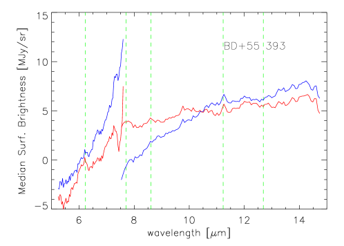
Figure 4: The effect of the ”dark settle” correction of the SL data is shown for the region around BD+55^∘ 393. The blue lines give the extracted SL spectra before correction and the red after correction. The green dashed vertical lines show the locations of the of the strong aromatic features.

4 Errors and Systematic Effects

The errors affecting the data arise from two sources: random measurement errors, and systematic errors due to instrumental effects. Our measurements are technically challenging as we are measuring the diffuse emission, requiring an absolute, not differential, measurement. The IRS instrument did not use a shutter, hence our measurements include the diffuse Milky Way emission combined with zodical emission and instrumental backgrounds/artifacts. This is in contrast to the usual differential measurements made with IRS where off source observations are subtracted from on source observations effectively removing the emissions in common (e.g., zodiacal and instrumental emissions). Figure 5 shows a detector image for Hi 188. The strong emission band at 11.3 $\mu$m is clearly present in the long wavelength (left) portion of the spectrum. It is also obvious that there is a non-uniform response in the spatial direction (perpendicular to the dispersion) for the short wavelength (middle) portion of the spectrum. This non-uniformity is most likely an instrumental effect, since it is present in all of the spectra, regardless of their location with respect to the Galaxy or the ecliptic.

These correlated errors are predominantly affect the SL1 spectra and depend on detector location. Because the sky is scanned by the observations, the same wavelength or location on the sky can be observed at different detector locations. This gives rise to large, correlated variations which are mostly detector based. These large variations result in large off-diagonal elements in the error covariance matrices and also create large contributions to the random component of the diagonal elements (which are typically reported as the mono-variate errors affecting the spectra).

To identify the correlated contributions, we performed principal axis decomposition of the SL2 error covariance matrices. These showed that most of the off-diagonal elements, and a large fraction of the diagonal elements, resulted from a few well defined functions that are most likely related to the cross-dispersion detector response seen in Figure 5.

Since it is much easier to manipulate and display mono-variate errors, and because the signatures of the correlated errors are broad band and unlike the lines we wish to analyze, we decided to correct the mono-variate errors for the correlated contributions. This was done by removing the contributions of the two largest principal axes from the diagonal elements of the error covariance matrices and then using these corrected diagonal elements for error weighting and significance analyses. This process was only done for the SL2 data, as the off-diagonal elements of the SL1 data were generally much smaller than the diagonal elements, indicating that the magnitudes of the diagonal elements were not strongly affected by correlated errors.

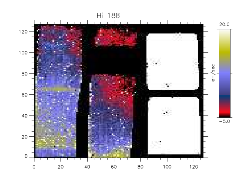
Figure 5: Image of the detector for a diffuse background observation near Hiltner 188. The 11.3 $\mu$m feature is clearly visible in the SL1 spectrum on the left side of the image near $y=65$, $0\leq x\leq 30$. The highly variable SL2 background is also apparent as the change in intensity across the SL2 spectrum which occupies $40\lesssim x\lesssim 70$

.

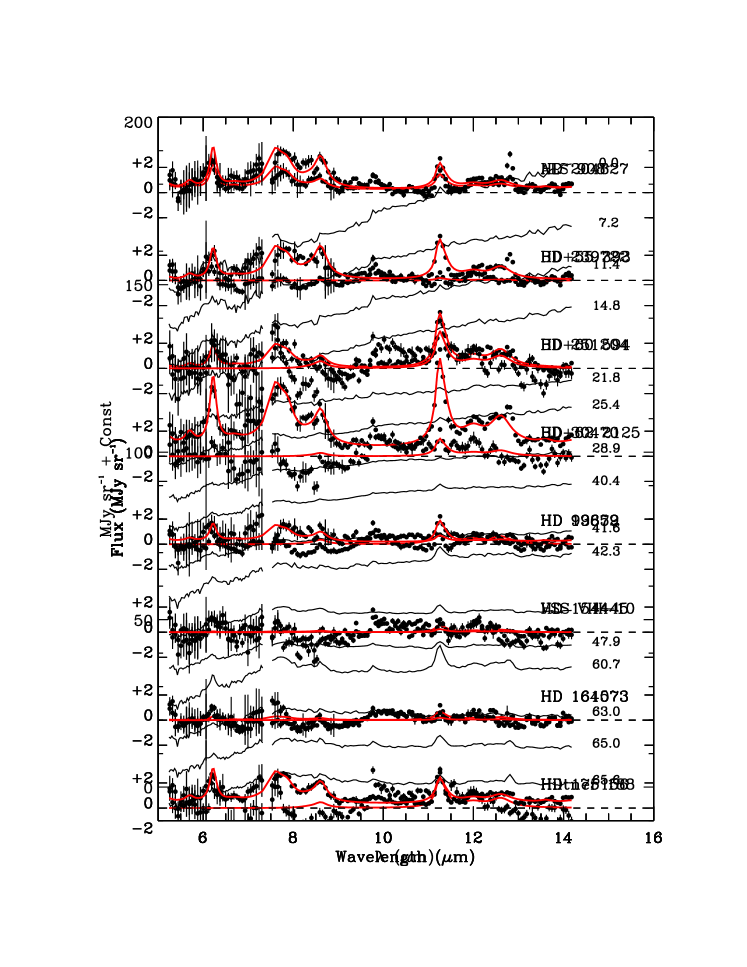
Figure 6: Spectra of the program stars in order of decreasing absolute value of ecliptic latitude, $|\beta|$, listed to the right of each spectrum. The strong dependence of the continuum slope between 8 and 14.5 $\mu$m on $|\beta|$ is clearly evident. Also note that the spectral feature near 6.2 $\mu$m is wider in spectra near the ecliptic plane. This appears to result from the strengthening of a zodiacal light feature near the 6.22 $\mu$m interstellar PAH feature.

Figure 7: Examples of spectra where, in each case, the upper plot is the observed spectrum with the continuum background fit shown, and the lower spectrum has the background subtracted. The circles are the locations of the points used to determine the background continuum.

5 Analysis

In this section, we first describe how we model the zodiacal light contribution to the observed spectra. We then introduce a simple model for the interstellar PAH emission lines. Next, we consider additional features that are present in the spectra but are not due to known PAH features. Finally, we define the model that we use to fit the observed spectra and give the details of how the model is used to extract quantitative information from the spectra.

5.1 Zodiacal light continuum

Figure 6 shows the spectra toward the program stars, arranged in order of the absolute magnitudes of their ecliptic latitude, $|\beta|$, with those at the smallest latitudes at the top. A few things are apparent. First, the overall slope of the continua increase with decreasing $|\beta|$. Second, the emission feature near 6.2 $\mu$m is wider for sight lines with small $|\beta|$.

To minimize the effects of the zodiacal light and to isolate and quantify the interstellar features, we remove the continuous background. This was done by fitting a spline to 6 points which appear to be free of emission features. These points are at 5.65, 6.75, 9.15, 10.90, 13.1, and 14.0 $\mu$m. Figure 7 shows 2 examples of spectra with and without the background subtracted.

5.2 The PAH model

While a few of the PAH features are distinct, most of the main features in the spectra are clearly blends. Rather than attempting to fit every possible emission feature in the spectra as an independent line, we adopt the positions, widths and relative strengths of the Drude profiles used in the Draine & Li (2007, DL07 hereafter)model as a starting point. However, instead of grouping the lines into ionized and neutral PAH and with and without CH stretch, we simply use all of the lines listed as ionized PAHs between 5 and 15 $\mu$m, and break them into 4 segments, centered around the four strongest observed features, i.e., $5.0\leq\lambda<7$, $7\leq\lambda<8$, $8\leq\lambda<9$, and $9\leq\lambda\leq 15$. We refer to these as the 6.2, 7.6, 8.5 and 11.3 $\mu$m PAH features, respectively.

When comparing the observed spectra to the models, it became apparent that a few of the lines had to be rescaled. Consequently, we increased the strength of the DL07 5.25 $\mu$m feature (which only has its red wing in our wavelength range) and the strength of their 11.99 $\mu$m feature by a factor of 2.5.

5.3 Unidentified features

Upon examining the continuum subtracted spectra, it became apparent that they contained three features not included in the DL07 model. Consequently, we include three non-PAH features in our model. These are: 1) a feature we represented as a Drude profile with $\lambda_{0}=6.03$ $\mu$m and $\gamma=0.20$, $D(6.03,0.29,\lambda)$, 2) a second feature we approximate as a Drude profile with $\lambda_{0}=7.20$ $\mu$m and $\gamma=0.25$, $D(7.20,0.25,\lambda)$, and 3) an asymmetric feature which we approximate as a $\chi^{2}$ distribution function with 5 degrees of freedom and its abscissa, $u$, scaled and shifted so that $\lambda=au+\lambda_{0}$, where $a=1/12$ and $\lambda_{0}=9.55$ $\mu$m, $\chi^{2}_{5}([\lambda-\lambda_{0}]/a)$. These parameters place the peak of the distribution near 9.8 $\mu$m. We refer to these three features as the 6.0, 7.2 and 9.8 $\mu$m features and discuss their possible physical origins in § 7.

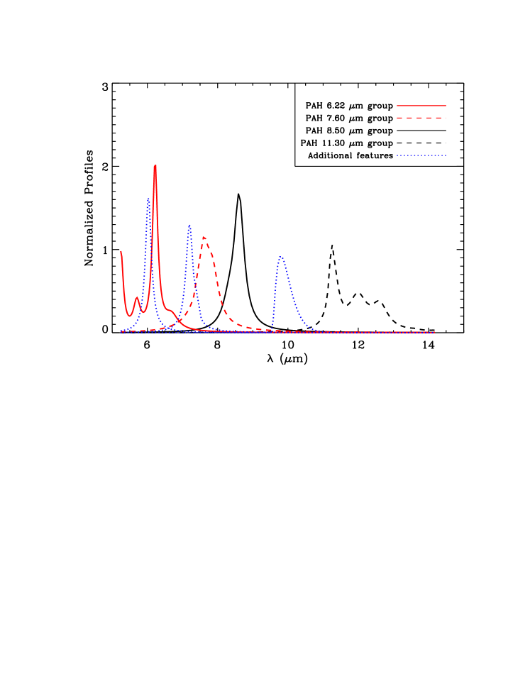
Figure 8: The 7 fitting functions adopted for our analysis. The four segments of the DL07 PAH model we use are shown as the solid red, dashed red, solid black and dashed black curves, which represent the 6.22, 7.6, 8.5 and 11.3 $\mu$m components, respectively. The 3 dotted blue curves are the 3 additional features at 6.0, 7.2 and 9.8 $\mu$m, which are described in the text.

5.4 The final model

When fitting our model to the observations, we first fit a continuum to each spectrum using the spline, described in §5.1, and then remove the continuum. The resulting curve is then fit to the model described above for seven free parameters, $c(\lambda_{i})$, where $\lambda_{i}=6.2,7.6,8.5,11.3,6.0,7.2,9.8$ $\mu$m, i.e.,

$$f(\lambda)=\sum_{i=1}^{4}c(\lambda_{i})\Phi(\lambda)_{i}+\sum_{i=5}^{6}c(\lambda_{i})D(\lambda_{i},\gamma_{i},\lambda)+c(\lambda_{7})\chi^{2}_{5}(\lambda)-s(\lambda)$$ (1)

where the $\Phi(\lambda)_{i}$ are the 4 segments of the DL07 model (modified as described above), the two $D(\lambda_{i},\gamma_{i},\lambda)$ and $\chi^{2}_{5}(\lambda)$ are the two Drude profiles and $\chi^{2}$ distribution described in the previous section and $s(\lambda)$ is the spline described in § 5.1, which is removed to place the model and the observations into the same form. The fitting functions are shown in Figure 8. Because the profiles are all normalized, the coefficients, $c(\lambda_{i})$, have units of MJy sr^-1. The appendix provides further details about the Drude profiles and explains how to recover the contribution of each one form the $c(\lambda_{i})$ fit parameters. Using these functions, and the errors derived in § 4, we performed non-linear least squares fits using the Interactive Data Language (IDL) procedure MPFIT developed by Markwardt (2009). If we did not have to subtract the spline in order to be consistent with the observations, we could simply use a linear regression to fit the PAH and other features. However, because removal of the spline from the fitting functions is required, it becomes a non-linear least squares problem.

As an example of the fitting, Figure 9 shows the fit to the sample mean, and the scaled components of the fit. Because zodiacal light contamination precludes our ability to determine the continuum of the observed spectra, the data have been adjusted to agree with the continuum implied by the fit. Specifically, the spline fit to the observed spectrum was removed and replaced with the spline fit to the model. While the overall fit to the strongest features is quite good, there are a few regions where our model does not fit very well. Specifically, these include the regions of the minima near 6.5, 9.4 and 10.5 $\mu$m, and the plateau between 12 and 13 $\mu$m. This is not too surprising since the major features are probably not perfect Drude profiles and several weaker features have probably been omitted. Nevertheless, the model appears to capture the strongest features in the spectrum quite well, providing quantitative measures of their strengths.

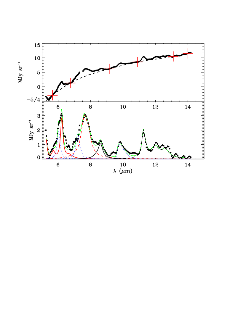
Figure 9: Top: The points are the sample mean spectrum (smoothed by 3 points) and the dashed curve is a spline fit to the 6 points indicated by the large crosses. Bottom: Green curve is an illustrative fit to the mean spectrum with its continuum adjusted to agree with the model. The solid, dashed red and black curves and dotted blue curves are the major model features, with the same color code as Figure 8. The relatively poor fit near 7 $\mu$m results because this region is near the poorly determined points at the edges of the SL1 and SL2 spectra.

Figure 10: Stacked display of observed emission (points) and one $\sigma$ error bars, along with our model fits. Each curve is labeled by the star along its line of sight.

Figure 11: Same as Figure 10.

6 Results

We begin this section with a presentation of the fits to the spectra and a description of a few of their properties. Next, we investigate the dependence of the model parameters on ecliptic latitude and then examine the coefficients relations to each other. Finally, we introduce a set of extinction measurements for the program stars and examine correlations between the extinction curve parameters and the parameters which describe the Spitzer spectra.

Table 2: Fit coefficients (in MJy sr^-1)

Star	$c(6.2)$	$c(7.6)$	$c(8.5)$	$c(11.3)$	$c(9.8)$	$c(6.0)$	$c(7.2)$
BD+55∘393	$0.92\pm 0.15$	$1.75\pm 0.10$	$0.38\pm 0.10$	$0.81\pm 0.05$	$1.39\pm 0.102$	$0.46\pm 0.32$	$1.12\pm 0.32$
Hiltner 188	$1.18\pm 0.14$	$2.83\pm 0.08$	$0.96\pm 0.08$	$2.51\pm 0.04$	$1.00\pm 0.085$	$0.25\pm 0.28$	$1.04\pm 0.28$
HD 13659	$0.98\pm 0.10$	$1.49\pm 0.07$	$0.25\pm 0.07$	$1.49\pm 0.07$	$1.19\pm 0.104$	$0.27\pm 0.21$	$1.12\pm 0.21$
BD+60∘594	$1.40\pm 0.23$	$2.93\pm 0.11$	$0.64\pm 0.11$	$3.83\pm 0.10$	$1.74\pm 0.190$	$0.34\pm 0.32$	$0.49\pm 0.32$
HD 30470	$1.78\pm 0.23$	$1.93\pm 0.13$	$0.53\pm 0.13$	$0.60\pm 0.18$	$2.01\pm 0.276$	$1.20\pm 0.68$	$1.77\pm 0.68$
HD 251204	$3.07\pm 0.46$	$4.96\pm 0.14$	$0.96\pm 0.14$	$1.75\pm 0.25$	$1.95\pm 0.335$	$1.82\pm 0.69$	$1.62\pm 0.69$
ALS 908	$0.95\pm 0.14$	$2.26\pm 0.08$	$0.55\pm 0.08$	$2.09\pm 0.04$	$1.65\pm 0.095$	$0.27\pm 0.33$	$1.39\pm 0.33$
HD 99872	$0.81\pm 0.28$	$2.14\pm 0.14$	$0.67\pm 0.14$	$1.45\pm 0.06$	$1.75\pm 0.140$	$0.21\pm 0.45$	$1.53\pm 0.45$
HD 154445	$1.42\pm 0.27$	$1.30\pm 0.00$	$0.00\pm 0.00$	$0.90\pm 0.11$	$0.86\pm 0.150$	$0.62\pm 0.44$	$1.10\pm 0.44$
HD 161573	$0.89\pm 0.13$	$1.50\pm 0.10$	$0.24\pm 0.10$	$0.28\pm 0.07$	$1.08\pm 0.113$	$0.50\pm 0.30$	$0.98\pm 0.30$
HD 164073	$1.18\pm 0.10$	$1.92\pm 0.12$	$0.50\pm 0.12$	$0.97\pm 0.08$	$1.72\pm 0.123$	$0.60\pm 0.31$	$1.12\pm 0.31$
HD 175156	$2.45\pm 0.23$	$4.13\pm 0.13$	$0.58\pm 0.13$	$1.31\pm 0.18$	$1.76\pm 0.261$	$1.16\pm 0.46$	$2.21\pm 0.46$
VSS VIII-10	$1.56\pm 0.21$	$1.01\pm 0.12$	$0.11\pm 0.12$	$0.00\pm 0.00$	$1.40\pm 0.227$	$0.94\pm 0.42$	$0.98\pm 0.42$
HD 204827	$1.00\pm 0.28$	$3.34\pm 0.14$	$1.27\pm 0.14$	$2.75\pm 0.07$	$1.19\pm 0.149$	$0.24\pm 0.42$	$0.91\pm 0.42$
HD 239722	$1.05\pm 0.21$	$3.09\pm 0.16$	$1.36\pm 0.16$	$3.51\pm 0.08$	$1.34\pm 0.152$	$0.11\pm 0.40$	$1.39\pm 0.40$
BD+62∘2125	$2.16\pm 0.25$	$5.85\pm 0.17$	$1.95\pm 0.17$	$6.80\pm 0.10$	$2.12\pm 0.154$	$0.33\pm 0.70$	$1.27\pm 0.70$

Table 2 lists the parameters that result from fits to the data using eq. (1). Figures 10 and 11 display the fits to the individual lines of sight and, as in Fig. 9, we display the fits using the model continuum derived for each one. A few features are worth emphasizing. Generally, the strength of the features scale with $E(B-V)$, but there are clear exceptions. For example, BD$+60^{\circ}594$ has a slightly smaller color excess than VSS VIII-10, but the PAH features are much stronger in BD$+60^{\circ}594$. In contrast, the features in the spectra toward HD 13659 and HD 161573 have similar strengths, even though their $E(B-V)$ differ by a factor of 4. Generally, the strengths of the PAH features appear to vary together, although there are a few exceptions. Specifically, for most sight lines, the 7.6 $\mu$m feature is only slightly stronger than the 11.3 $\mu$m feature, but toward HD 239722 and HD 175156, the peak of the 7.6 $\mu$m feature is far stronger. However, we shall argue below that this may actually result from contamination of the 7.6 $\mu$m feature in HD 251204 and HD 175156 by zodiacal emission. Finally, we point out that the [Ne ii] 12.81 $\mu$m emission line is present in the sight lines toward HD 204827 and HD 239722, both in the open cluster Tr 37, and probably present in the line of sight to BD$+62^{\circ}$ 2125, a member of Cep OB3.

We begin our search for correlations by examining the relations of the unidentified features to the absolute value of ecliptic latitude, $|\beta|$. Figure 12 presents these coefficients plotted against $|\beta|$ for each line of sight. There is no obvious correlation for the 9.8 $\mu$m feature, and the 7.2 $\mu$m feature may be weakly correlated with $|\beta|$. However, the 6.0 $\mu$m line is strongly correlated with $|\beta|$.

Figure 12: Coefficients of the unidentified features plotted against the absolute value of the ecliptic latitude of their line of sight.

Figure 13 shows the strengths of the four PAH features plotted against each other. Clearly, the 6.2 $\mu$m PAH feature is not correlated with the others, but the 7.6, 8.5 and 11.3 $\mu$m PAH features are all strongly related to one another. On the other hand, Figure 14 shows that the 6.2 $\mu$m PAH feature is correlated with 6.0 $\mu$m feature, which has been shown to be related to the zodiacal light Reach et al. (2003). It is likely that the reason the 6.2 $\mu$m feature is not correlated with the other PAH features is that the values we derive for its strength are entangled with those for the 6.0 $\mu$m feature.

The two points shown as open circles in fig. 13 deviate from the others for plots involving $c(7.6)$. These are for HD 251204 and and HD 175146. They have the smallest $|\beta|$ values in our sample, $0.0^{\circ}$ and $7.2^{\circ}$, respectively (see, Table 1). This makes their spectra the most susceptible to zodiacal light contamination. Thus, we suspect that zodiacal light affects not only $c(6.2)$, but probably $c(7.6)$ as well for these two stars.

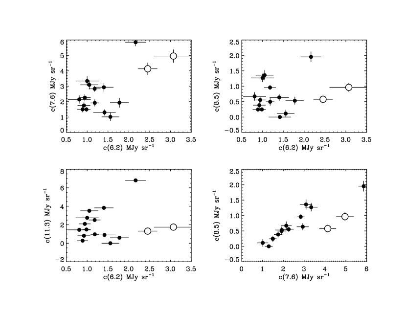
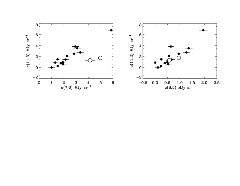
Figure 13: The strengths of the four PAH features plotted against each other. One $\sigma$ error bars are also shown. Open circles are for stars with $|\beta|<10^{\circ}$.

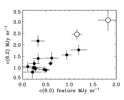
Figure 14: Correlation between the 6.2 $\mu$m PAH feature and the 6.0 $\mu$m unidentified feature. Open circles are for stars with $|\beta|<10^{\circ}$.

We now turn to the extinction parameters. Some of these are the coefficients from eq. (2) in Fitzpatrick & Massa (2007), which we denote as $a_{i}$. Specifically, we use the following parameters: $E(B-V)$ (the color excess), $A(V)=E(B-V)\times R(V)$ (the total extinction in the $V$ band), $a_{2}\times E(B-V)$ (a measure of the slope of the UV extinction), $a_{4}\times E(B-V)$ (a measure of the curvature of the far-UV extinction), and $A(2175)$ (the bump area), which is given by

$$A(2175)=\frac{\pi a_{3}}{2\gamma}E(B-V)$$ (2)

The observed values of these parameters for the program stars are listed in Table 3

Table 3: Extinction Properties

Star	$E(B-V)$	$A(2175)$	$A(V)$	$a_{2}E(B-V)$
BD+55∘393	0.26	1.172	0.738	0.179
Hiltner 188	0.66	3.487	1.888	0.667
HD 13659	0.80	2.631	1.984	0.920
BD+60∘594	0.65	3.579	1.729	0.507
HD 30470	0.34	1.879	1.108	0.180
HD 251204	0.76	3.523	2.333	0.555
ALS 908	0.65	3.241	1.943	0.455
HD 99872	0.32	2.267	0.957	0.067
HD 154445	0.40	2.734	1.180	0.140
HD 161573	0.20	1.070	0.620	0.072
HD 164073	0.21	0.504	1.121	0.109
HD 175156	0.35	1.615	1.095	0.438
VSS VIII-10	0.74	1.427	3.093	0.673
HD 204827	1.09	4.834	2.681	1.330
HD 239722	0.88	5.014	2.297	0.766
BD+62∘2125	0.91	4.871	2.466	0.692

When comparing dust absorption and emission, it is important to bare in mind that the absorption depends simply on the column density of absorbers along the line of sight. In contrast, the emission also depends on the ambient radiation field along the line of sight and the uniformity of the emission over the solid angle subtended by the observing aperture.

Our method of selecting targets maximizes the chance that they are beyond the vast majority of dust along the line of sight and do not interact with it. Nevertheless, the sight line may encounter complex regions where the radiation field is very different from the mean and the spatial distribution of the dust is highly variable.

The uniformity of the radiation field over the solid angle of the aperture can be evaluated by examining the variance in the 6 slit positions observed for each star (see figure 3). The combined SL1 and SL2 observations sample a region centered on the star that is roughly $215^{\prime\prime}$ in $x$ and $45^{\prime\prime}$ in $y$. Figure 15 shows two sets of these observations; one is for a star whose whose deviations are typical and one for BD$+62^{\circ}$ 2125, which has largest systematic deviations in the sample. It is clear that one spectrum has considerably more emission over the region $8\leq\lambda\leq 10$ $\mu$m. Nevertheless, even in this extreme case, the overall strength of the major PAH features are not strongly affected.

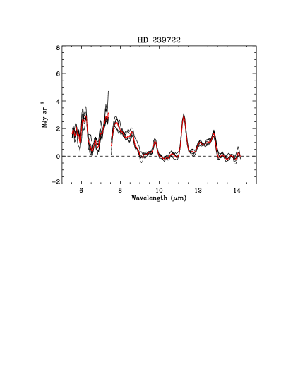
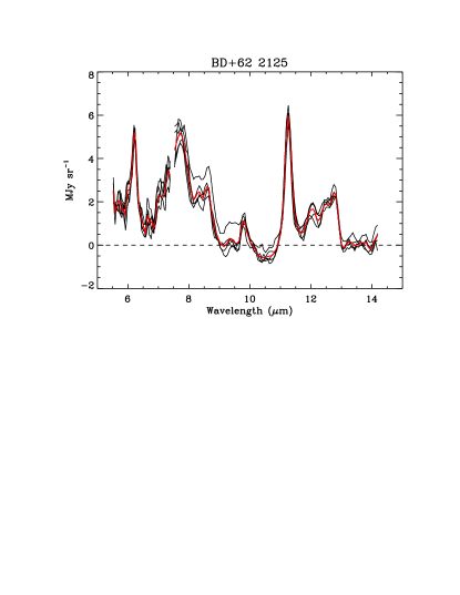
Figure 15: SL1 and SL2 spectra for all of the different aperture positions (black) and the mean (red) for HD 239722 (left) and BD$+62^{\circ}$ 2125. All spectra were smoothed by 3 points. The scatter in the HD 239722 spectra is typical of the stars in our sample. In contrast, BD$+62^{\circ}$ 2125 is the only star in the sample with a spectrum that appears systematically different from the others.

Figure 16 shows how the four PAH features are related to $A(2175)$. We see that $A(2175)$ is strongly correlated to the 8.5 and 11.3 $\mu$m features, somewhat correlated with the 7.6 $\mu$m feature, but uncorrelated to the 6.2 $\mu$m feature. However, we have already shown that the 6.2 $\mu$m data are contaminated by zodiacal emission, so this last result is not surprising. Further, when the two stars with $|\beta|<10^{\circ}$ (again shown as open circles) are omitted, the relationship between $c(6.7)$ and $A(2175)$ is also quite strong.

Figure 17 presents the relations between the total optical extinction, $A(V)$, and the PAH parameters. In this case, no strong correlations are present. Together with the previous plot, these results indicate that the PAH emission is strongly correlated with whatever causes the 2175 Å absorption, but not with the overall line of sight extinction.

We also examined correlations between the PAH emission features and the dust temperature, as determined by Schlegel et al. (1998). However, no significant relations were found.

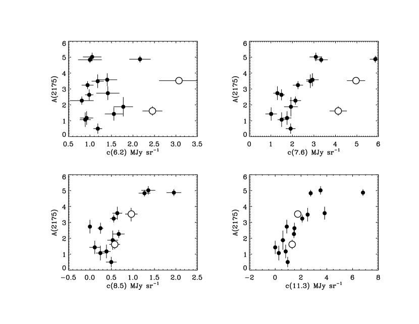
Figure 16: The area of the 2175 Å bump plotted against the strengths of the four PAH features, with $1\sigma$ error bars. Open circles are for stars with $|\beta|<10^{\circ}$.

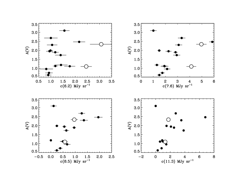
Figure 17: $A(V)$  plotted against the strengths of the four PAH features, with $1\sigma$ error bars. Open circles are for stars with $|\beta|<10^{\circ}$.

7 Discussion

In this section, we summarize and discuss our results. We begin with the results for the features not included in the DL07 model.

• The 6.0 $\mu$m feature is strongly related to ecliptic latitude, implying that it is related to the zodiacal light. Furthermore, it seems to be present in some of the zodiacal light spectra presented in Reach et al. (2003). It is also correlated with the 6.2 $\mu$m PAH feature. This suggests that the 6.2 $\mu$m and 6.0 $\mu$m measurements are entangled, and probably accounts for lack of correlation between the 6.2 $\mu$m feature and the other PAH features.

• The 7.2 $\mu$m feature is weakly correlated to $|\beta|$ and unrelated to anything else. We suspect that it is primarily an adjustment which accounts for any residual discontinuity between the SL1 and SL2 caused by the ”dark settle” effect described in § 3. Errors in this discontinuity may be larger when the zodiacal emission is stronger, which could account for the weak correlation with $|\beta|$.

• The 9.8 $\mu$m emission feature is near the 9.7 $\mu$m silicate absorption feature, suggesting a possible relation. However, it also appears to be present in the zodiacal light spectra presented in Reach et al. (2003), but it is not significantly correlated with ecliptic latitude, so its origin is uncertain.

• The [Ne ii] 12.81 $\mu$m emission line is present in three of the sight lines in Figure 11. It is quite strong in HD 204827 and HD 2397223 (both members of Tr 37) and a bit weaker toward BD$+62^{\circ}2125$, a member of Cep OB3. Both of these regions are sites of recent and ongoing star formation.

We now summarize our results for the PAH features.

• The 8.5 and 11.3 $\mu$m PAH features at are strongly related to one another.

• 7.8 $\mu$m PAH feature is also strongly correlated with the 8.5 and 11.3 $\mu$m features with the exception of two stars. These have the smallest $|\beta|$ in the sample and we suspect that this is due to zodical light contamination (possibly from the 7.2 $\mu$m feature).

• The 6.2 $\mu$m PAH feature does not correlate well with the other PAH features. This is likely because its values are entangled with the nearby 6.0 $\mu$m unidentified, possible zodiacal, feature.

• The bump area, $A(2175)$, is strongly correlated with the 8.5 and 11.3 $\mu$m features, less strongly correlated with 7.6 $\mu$m feature, and uncorrelated to the 6.2 $\mu$m feature, mimicking how the PAH features are related to each other. The one star whose data deviate somewhat from this relation is BD$+62^{\circ}2125$, whose line of sight (which passes through the star forming region Cep OB3) seems to have more PAH intensity than expected for its $A(2175)$.

• The total extinction at optical wavelengths, $A(V)$, is not correlated to the strengths of the PAH parameters. This argues that the relation between $A(2175)$ and the strengths of the PAH features is due to a similarity in the kind of dust along the line of sight and not just the amount.

Our first main finding is that the 7.6, 8.5 and 11.3 $\mu$m PAH features are strongly correlated. The correlations among the PAH lines indicate that the intensities of these features respond similarly. Recall that there are cases where the amount of interstellar dust, as measured by $E(B-V)$, is quite large and the emission features are weak, and vice versa. Thus, whatever produces these features, affects all three in the same way. Thus, it appears that the ratios of the amplitudes of the PAH features are roughly constant for our lines of sight through the relatively diffuse interstellar medium. In fact, simple regressions of $c(7.6)$ and $c(8.5)$ on $c(11.3)$, with the intercepts forced to 0, give slopes (ratios) of $c(7.6)/c(11.3)=0.96$ (omitting HD 251204 and HD 175156) and $c(8.5)/c(11.3)=0.31$ (including all stars). Consequently, for $c(7.6)$, $c(8.5)$ and $c(11.3)$, the line of sight environment affects their brightness, but not their ratios.

The second main finding is that $A(2175)$ is strongly correlated with the strength of the PAH emission lines. In some ways, this strong correlation is surprising. This is because $A(2175)$ is a direct measure of the total column density of 2175 Å absorbers along the line of sight, while the PAH emission depends not only on the number of emitters, but also on the local radiation field at each point along the line of sight. Thus, even if the carriers of the 2175 Å feature and the PAH emitters were identical, this would not guarantee a correlation between $A(2175)$ and the strength of the PAH emission. For such a relation to occur, either the diffuse radiation field along each line of sight must be roughly constant, or the conditions that create the 2175 Å absorbers and the PAH emitters are both directly related the ambient radiation field, perhaps through a two step process of the sort described by Witt et al. (2006) in a much different context.

$$D(\lambda_{i},\gamma_{i},\lambda)_{0}=\frac{\gamma_{i}\lambda_{i}}{(\lambda/\lambda_{i}-\lambda_{i}/\lambda)^{2}+\gamma_{i}^{2}}$$ (1)

In this paper, we use normalized Drude profiles,

$$D(\lambda_{i},\gamma_{i},\lambda)=\frac{D(\lambda_{i},\gamma_{i})_{0}}{\int_{0}^{\infty}D(\lambda_{i},\gamma_{i})_{0}}$$ (2)

The PAH fitting functions, $\Phi(\lambda)_{i}$, used in equation (1) are composed of several normalized Drudes, multiplied by coefficients, $b_{i,j}$, which are proportional to their relative contributions in the DL07 models. Since the $\Phi(\lambda)_{i}$ are normalized to unity, we have $\sum_{j=1}^{N}b_{i,j}=1$, for all $i$, and

$$\Phi(\lambda)_{i}=\sum_{j=1}^{N}b_{i,j}D(\lambda_{i,j},\gamma_{i,j},\lambda)$$ (3)

The values of $\lambda_{i,j}$, $\gamma_{i,j}$ and $b_{i,j}$ are given in Table 4. As a result, it is possible to use the $c(\lambda_{i})$ fit parameters given in equation (1) together with the $b_{i,j}$ to determine the contribution of each Drude to the fit, i.e., $c(\lambda_{i})\;b_{i,j}\;D(\lambda_{i,j},\lambda_{i,j},\lambda)$ gives the contribution of the $j^{th}$ Drude to $\Phi(\lambda)_{i}$.

Table 4: $\Phi(\lambda)_{i}$ Component Parameters

$\lambda_{i}\;\;\;$	$\lambda_{i,j}$	$\gamma_{i,j}$	$b_{i,j}$
6.2 $\mu$m	5.250	0.0300	0.22700
	5.700	0.0400	0.11400
	6.220	0.0284	0.53600
	6.690	0.0700	0.12300
7.6 $\mu$m	7.417	0.1260	0.24000
	7.598	0.0440	0.38900
	7.850	0.0530	0.37100
8.6 $\mu$m	8.330	0.0520	0.18900
	8.610	0.0390	0.81100
11.3 $\mu$m	11.23	0.0100	0.07320
	11.30	0.0290	0.33500
	11.99	0.0500	0.34900
	12.61	0.0435	0.23400
	13.60	0.0200	0.00444
	14.19	0.0250	0.00480

References

- Allamandola et al. (1985) Allamandola, L. J., Tielens, A. G. G. M., & Barker, J. R. 1985, ApJ, 290, L25, doi: 10.1086/184435
- Bakes et al. (2001) Bakes, E. L. O., Tielens, A. G. G. M., & Bauschlicher, Charles W., J. 2001, ApJ, 556, 501, doi: 10.1086/321501
- Blasberger et al. (2017) Blasberger, A., Behar, E., Perets, H. B., Brosch, N., & Tielens, A. G. G. M. 2017, ApJ, 836, 173, doi: 10.3847/1538-4357/aa5b8a
- Chiar et al. (2013) Chiar, J. E., Tielens, A. G. G. M., Adamson, A. J., & Ricca, A. 2013, ApJ, 770, 78, doi: 10.1088/0004-637X/770/1/78
- Clayton et al. (2003) Clayton, G. C., Gordon, K. D., Salama, F., et al. 2003, ApJ, 592, 947, doi: 10.1086/375771
- Draine & Li (2007) Draine, B. T., & Li, A. 2007, ApJ, 657, 810, doi: 10.1086/511055
- Draine et al. (2007) Draine, B. T., Dale, D. A., Bendo, G., et al. 2007, ApJ, 663, 866, doi: 10.1086/518306
- Fan et al. (2019) Fan, H., Hobbs, L. M., Dahlstrom, J. A., et al. 2019, ApJ, 878, 151, doi: 10.3847/1538-4357/ab1b74
- Fitzpatrick & Massa (1986) Fitzpatrick, E. L., & Massa, D. 1986, ApJ, 307, 286, doi: 10.1086/164415
- Fitzpatrick & Massa (1988) —. 1988, ApJ, 328, 734, doi: 10.1086/166332
- Fitzpatrick & Massa (1990) —. 1990, ApJS, 72, 163, doi: 10.1086/191413
- Fitzpatrick & Massa (2005) —. 2005, AJ, 130, 1127, doi: 10.1086/431900
- Fitzpatrick & Massa (2007) —. 2007, ApJ, 663, 320, doi: 10.1086/518158
- Gaia Collaboration (2018) Gaia Collaboration. 2018, VizieR Online Data Catalog, I/345
- Hensley & Draine (2020) Hensley, B. S., & Draine, B. T. 2020, ApJ, 895, 38, doi: 10.3847/1538-4357/ab8cc3
- Houck et al. (2004) Houck, J. R., Roellig, T. L., van Cleve, J., et al. 2004, ApJS, 154, 18, doi: 10.1086/423134
- Jenniskens & Desert (1993) Jenniskens, P., & Desert, F. X. 1993, A&A, 275, 549
- Joblin et al. (1992) Joblin, C., Leger, A., & Martin, P. 1992, ApJ, 393, L79, doi: 10.1086/186456
- Kemper et al. (2004) Kemper, F., Vriend, W. J., & Tielens, A. G. G. M. 2004, ApJ, 609, 826, doi: 10.1086/421339
- Li & Draine (2001) Li, A., & Draine, B. T. 2001, ApJ, 554, 778, doi: 10.1086/323147
- Linsky et al. (2006) Linsky, J. L., Draine, B. T., Moos, H. W., et al. 2006, ApJ, 647, 1106, doi: 10.1086/505556
- Malloci et al. (2007) Malloci, G., Joblin, C., & Mulas, G. 2007, A&A, 462, 627, doi: 10.1051/0004-6361:20066053
- Malloci et al. (2008) Malloci, G., Mulas, G., Cecchi-Pestellini, C., & Joblin, C. 2008, A&A, 489, 1183, doi: 10.1051/0004-6361:200810177
- Malloci et al. (2004) Malloci, G., Mulas, G., & Joblin, C. 2004, A&A, 426, 105, doi: 10.1051/0004-6361:20040541
- Markwardt (2009) Markwardt, C. B. 2009, in Astronomical Society of the Pacific Conference Series, Vol. 411, Astronomical Data Analysis Software and Systems XVIII, ed. D. A. Bohlender, D. Durand, & P. Dowler, 251. https://arxiv.org/abs/0902.2850
- Massa et al. (2020) Massa, D., Fitzpatrick, E. L., & Gordon, K. D. 2020, ApJ, 891, 67, doi: 10.3847/1538-4357/ab6f01
- Mattioda et al. (2020) Mattioda, A. L., Hudgins, D. M., Boersma, C., et al. 2020, ApJS, 251, 22, doi: 10.3847/1538-4365/abc2c8
- Peeters et al. (2004) Peeters, E., Mattioda, A. L., Hudgins, D. M., & Allamandola, L. J. 2004, ApJ, 617, L65, doi: 10.1086/427186
- Potapov et al. (2021) Potapov, A., Bouwman, J., Jäger, C., & Henning, T. 2021, Nature Astronomy, 5, 78, doi: 10.1038/s41550-020-01214-x
- Reach et al. (2003) Reach, W. T., Morris, P., Boulanger, F., & Okumura, K. 2003, Icarus, 164, 384, doi: 10.1016/S0019-1035(03)00133-7
- Salama & Allamandola (1992) Salama, F., & Allamandola, L. J. 1992, ApJ, 395, 301, doi: 10.1086/171652
- Salama et al. (1995) Salama, F., Joblin, C., & Allamandola, L. J. 1995, Planet. Space Sci., 43, 1165, doi: 10.1016/0032-0633(95)00051-6
- Sandstrom et al. (2012) Sandstrom, K. M., Bolatto, A. D., Bot, C., et al. 2012, ApJ, 744, 20, doi: 10.1088/0004-637X/744/1/20
- Schlegel et al. (1998) Schlegel, D. J., Finkbeiner, D. P., & Davis, M. 1998, ApJ, 500, 525, doi: 10.1086/305772
- Smith et al. (2007) Smith, J. D. T., Armus, L., Dale, D. A., et al. 2007, PASP, 119, 1133, doi: 10.1086/522634
- Speck et al. (2011) Speck, A. K., Whittington, A. G., & Hofmeister, A. M. 2011, ApJ, 740, 93, doi: 10.1088/0004-637X/740/2/93
- Steglich et al. (2011) Steglich, M., Bouwman, J., Huisken, F., & Henning, T. 2011, ApJ, 742, 2, doi: 10.1088/0004-637X/742/1/2
- Steglich et al. (2012) Steglich, M., Carpentier, Y., Jäger, C., et al. 2012, A&A, 540, A110, doi: 10.1051/0004-6361/201118618
- Steglich et al. (2010) Steglich, M., Jäger, C., Rouillé, G., et al. 2010, ApJ, 712, L16, doi: 10.1088/2041-8205/712/1/L16
- Valencic et al. (2004) Valencic, L. A., Clayton, G. C., & Gordon, K. D. 2004, ApJ, 616, 912, doi: 10.1086/424922
- van Breemen et al. (2011) van Breemen, J. M., Min, M., Chiar, J. E., et al. 2011, A&A, 526, A152, doi: 10.1051/0004-6361/200811142
- van Leeuwen (2007) van Leeuwen, F. 2007, A&A, 474, 653, doi: 10.1051/0004-6361:20078357
- Vermeij et al. (2002) Vermeij, R., Peeters, E., Tielens, A. G. G. M., & van der Hulst, J. M. 2002, A&A, 382, 1042, doi: 10.1051/0004-6361:20011628
- Werner et al. (2004) Werner, M. W., Uchida, K. I., Sellgren, K., et al. 2004, ApJS, 154, 309, doi: 10.1086/422413
- Witt et al. (2006) Witt, A. N., Gordon, K. D., Vijh, U. P., et al. 2006, ApJ, 636, 303, doi: 10.1086/498052
- Zubko et al. (2004) Zubko, V., Dwek, E., & Arendt, R. G. 2004, ApJS, 152, 211, doi: 10.1086/382351