Generalized Binary Search Network for Highly-Efficient Multi-View Stereo

Abstract

Multi-view Stereo (MVS) with known camera parameters is essentially a 1D search problem within a valid depth range. Recent deep learning-based MVS methods typically densely sample depth hypotheses in the depth range, and then construct prohibitively memory-consuming 3D cost volumes for depth prediction. Although coarse-to-fine sampling strategies alleviate this overhead issue to a certain extent, the efficiency of MVS is still an open challenge. In this work, we propose a novel method for highly efficient MVS that remarkably decreases the memory footprint, meanwhile clearly advancing state-of-the-art depth prediction performance. We investigate what a search strategy can be reasonably optimal for MVS taking into account of both efficiency and effectiveness. We first formulate MVS as a binary search problem, and accordingly propose a generalized binary search network for MVS. Specifically, in each step, the depth range is split into 2 bins with extra 1 error tolerance bin on both sides. A classification is performed to identify which bin contains the true depth. We also design three mechanisms to respectively handle classification errors, deal with out-of-range samples and decrease the training memory. The new formulation makes our method only sample a very small number of depth hypotheses in each step, which is highly memory efficient, and also greatly facilitates quick training convergence. Experiments on competitive benchmarks show that our method achieves state-of-the-art accuracy with much less memory. Particularly, our method obtains an overall score of 0.289 on DTU dataset and tops the first place on challenging Tanks and Temples advanced dataset among all the learning-based methods. The trained models and code will be released at https://github.com/MiZhenxing/GBi-Net.

1 Introduction

Multi-view Stereo (MVS) is a long-standing and fundamental topic in computer vision, which aims to reconstruct 3D geometry of a scene from a set of overlapping images [9, 32, 10, 26, 35]. With known camera parameters, MVS matches pixels across images to compute dense correspondences and recover 3D points, which is essentially a 1D search problem [8]. A depth map is widely used as 3D representation due to its regular format. To overcome the issue of coarse matching in previous purely geometry-based methods, recent learning-based MVS methods [14, 21, 41, 42] designed deep networks for dense depth prediction to significantly advance traditional pipelines.

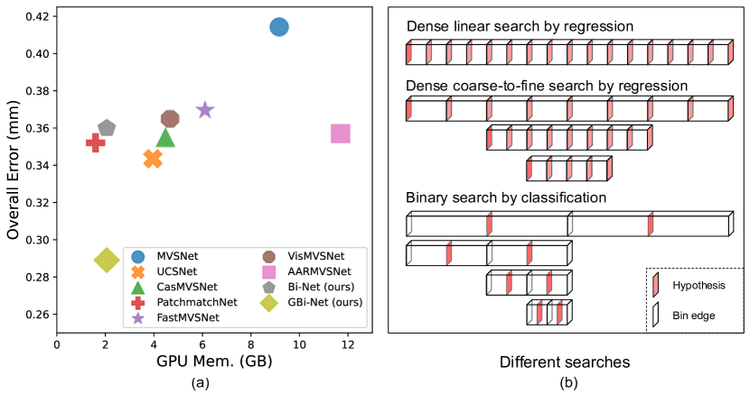
Figure 1: (a) Comparison with previous state-of-the-art learning-based MVS methods [41, 33, 5, 11, 44, 45, 34] on DTU [2]. The relationship between the overall error and the GPU memory overhead with image size $1152\times 1600$ and image number $5$. (b) Comparison of the previous dense search and the proposed binary search.

For instance, MVSNet [41] and RMVSNet [42] propose to construct 3D cost volumes from 2D image features with dense depth hypotheses. A 3D cost volume is a 5D tensor and is typically regularized by a 3D Convolutional Neural Network (CNN) or a Recurrent Neural Network (RNN) for depth prediction.

The importance of 3D cost volume regularization for accurate depth prediction has been confirmed by other works [4, 5, 11]. However, a severe problem is that 3D cost volumes are highly memory-consuming. Existing works made significant efforts to address this issue via decreasing the resolution of feature maps [41], using a coarse-to-fine strategy that gradually increases resolution of feature maps while decreasing the depth hypothesis number [4, 5, 11], and removing expensive 3D CNN or RNN [33, 40]. Although the memory can be alleviated to some extent, relatively lower accuracy is commonly observed. The size of 3D cost volume, specifically the depth hypothesis number, plays a dominant role in causing a large memory footprint.

Due to the significance of 3D cost volumes in both model efficiency and effectiveness, a critical question naturally arises: what is a minimum volume size to secure satisfactory accuracy while maintaining as small as possible the memory overhead? In this work, we investigate this question by exploring from a perspective of discrete search strategies, to identify a minimal depth hypotheses number, a key factor in 3D cost volumes. As shown in Fig. 1b, the vanilla MVSNet [41] can be seen as a dense search method that checks all depth hypotheses similar to a linear search in a parallel manner. The coarse-to-fine methods [11, 5] perform a multi-granularity search, which starts from a coarse level and gradually refines the prediction. However, these two types of methods both consider dense search in each stage. We argue that the dense search does not necessarily guarantee better accuracy due to a much larger prediction space and significantly increases model complexity, leading to higher optimization difficulty in model training.

To explore a reasonably optimal search strategy, we first formulate MVS as a binary search problem, which can remarkably reduce the cost volume size to an extremely low bound. It performs comparisons and eliminates half of the search space in each stage (see Fig. 1b), and can convergence quickly to a fine granularity within logarithmic stages. In contrast to regression-based methods, which directly sample depth values from the depth range, we first divide the depth range into 2 bins. In our design, the ‘comparisons’ by the network is to determine which bin contains the true depth value via performing a binary discrete classification. We use center points of the two bins to represent them and construct 3D cost volumes. The binary search offers superior efficiency, while it also brings an issue of the network classification error (i.e. prediction out of bins). The error can be accumulated from each search stage causing unstable optimization gradients and relatively low accuracy.

To tackle this issue, we further design three effective mechanisms, and accordingly propose a generalized binary search deep network, termed as GBi-Net, for highly efficient MVS. The first mechanism is that we pad two error tolerance bins on the two sides to reduce the prediction error of out of bins. The second mechanism is for training. If the network generates an error of prediction out of bins for a pixel at a search stage, we stop the forward pass of this pixel in the next stage, and the gradients at this stage are not used to update the network. Extensive experiments show that the proposed GBi-Net can largely decrease the size of 3D cost volumes for a significantly efficient network, and more importantly, without any trade-off on the depth prediction performance. The third is efficient gradient updating. It updates the network parameters immediately at each search stage without accumulating across different stages as most works do. It can largely reduce the training memory while maintaining the performance. Our method achieves state-of-the-art performance on different competitive datasets including DTU [2] and Tanks & Temples [17]. Notably, on DTU, we achieve an overall score of 0.289 (lower is better), remarkably improving the previous best performing method, and also obtain a memory efficiency improvement of 48.0% compared to UCSNet [5] and 54.1% compared to CasMVSNet [11] (see Fig. 1a).

In summary, our contribution is three-fold:

• We investigate efficient MVS from a perspective of search strategies, and propose a discrete binary search method for MVS (Bi-Net) which can vastly decrease the memory usage of 3D cost volumes.

• We design a highly-efficient generalized binary search network (GBi-Net) via further designing three mechanisms (i.e. padding error tolerance bins, gradients masking, and efficient gradient updating) with the binary search to avoid error accumulation of false network predictions and improve efficiency.

• We evaluate our method on several challenging MVS datasets and significantly advance existing state-of-the-art methods in terms of both the depth prediction accuracy and the memory efficiency.

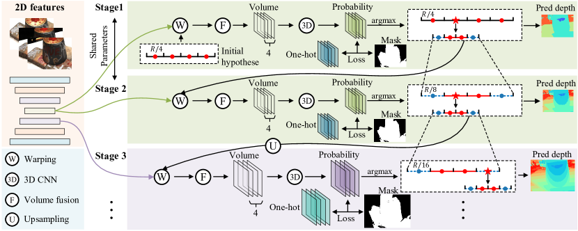
Figure 2: The multi-stage framework of our GBi-Net. The 2D CNNs first extract 2D feature maps. Then a 3D cost volume is constructed and fused by differentiable warping and only $4$ depth hypotheses. The cost volume is regularized by 3D CNNs and gets a probability volume for loss calculation with one-hot labels and training masks. We select the depth bin at current stage using $argmax$ operation. Then we update the depth hypotheses for the next stage with our proposed Generalized Binary Search.

2 Related Work

We review the most related works in the literature from two aspects, i.e. traditional MVS and learning-based MVS.

Traditional Multi-View Stereo. In 3D reconstruction, various 3D representations are used, such as volumetric representation [18, 27], point cloud [9, 19], mesh [6, 16, 29, 30] and depth map [10, 26, 3]. In MVS[23, 26, 35], depth maps have shown advantages in robustness, efficiency. They estimate a depth map of each reference image and fuse them into one 3D point cloud. For instance, COLMAP [26] simultaneously estimates pixel-wise view selection, depth, and surface normal. ACMM [35] leverages a multi-hypothesis joint voting scheme for view selection from different candidates. These existing methods perform modeling of occlusion, illumination across neighboring views for depth estimation. Although stable results can be achieved, high matching noise and poor correspondence localization in complex scenes are still severe limitations. Thus, our method mainly focuses on developing a deep learning-based MVS pipeline to advance the estimation performance.

Learning-based Multi-View Stereo. Deep learning-based MVS methods [15, 13, 41, 34] recently have achieved remarkable performance. Deep learning-based methods usually utilize Deep CNNs to estimate a dense depth map. Recently, 3D cost volumes have been widely used in MVS [41, 33, 45, 37]. As a pioneering method, MVSNet [41] constructs the 3D cost volume from feature warping and regularizes the cost volume with 3D CNNs for depth regression. The main problem of vanilla MVSNet is the large memory consumption of the 3D cost volume. Recurrent MVSNet architectures [42, 38, 34] leverage recurrent networks to regularize cost volumes, which can decrease the memory usage to some extent in the testing phase. However, the major overhead from the 3D cost volumes is not specifically addressed by these existing methods.

To reconstruct hig-resolution depth maps meanwhile obtaining a memory-efficient cost volume, cascade-based pipelines are proposed [11, 5, 39], considering a coarse-to-fine dense search strategy to gradually refine the depths. For instance, CasMVSNet [11] utilizes coarse feature maps and depth hypotheses in the first stage for coarse depth prediction, and then upsamples depth maps and narrows the depth range for fine-grained prediction in the next stage. Patchmatchnet  [33] learns adaptive propagation and evaluation for depth hypotheses. It removes heavy regularization of 3D cost volumes to achieve an efficient model while it makes a significant trade-off between efficiency and accuracy.

However, these existing works still consider a dense search in each regression stage. The memory overhead on the expensive 3D cost volume is clearly not optimized, while the proposed method targets highly efficient MVS with the designed binary search network, which largely advances the model efficiency, and more importantly, without sacrificing any depth prediction performance.

3 The Proposed Approach

In this section, we introduce the detailed structure of the proposed Generalized Binary Search Network (GBi-Net) for highly-efficient MVS. The overall framework is depicted in Fig. 2. It mainly consists of two parts, i.e. a 2D CNN network for learning visual image representations, and the generalized binary search network for iterative depth estimation. The GBi-Net contains $K$ search stages. In each search stage, we first compute 3D cost volumes by differentiable warping between the reference and source feature map in a specific corresponding scale. Then 3D cost volumes are regularized by 3D CNNs for depth label prediction. The Generalized Binary Search is responsible for initializing and updating depth hypotheses according to the predicted labels iteratively. In every two stages, the networks deal with the same scale of feature maps, and the network parameters are shared. Finally, one-hot labels for training the whole network are computed from ground-truth depth maps. In the next, we first introduce the 2D image encoder in Sec. 3.1 and the 3D cost volume regularization in Sec. 3.2. Then, we elaborate on details about our proposed Binary Search for MVS and Generalized Binary Search for MVS in Sec. 3.3 and Sec. 3.4, respectively. Finally, we present the overall network optimization in Sec. 3.5.

3.1 Image Encoding

The input consists of $N$ images $\{\mathbf{I}_{i}\}_{i=0}^{N-1}$. $\mathbf{I}_{0}$ is a reference image and $\{\mathbf{I}_{i}\}_{i=1}^{N-1}$ is a set of $N-1$ source images. We use Feature Pyramid Network (FPN) [20] as an image encoder to learn generic representation for the images with shared network parameters. From FPN, we obtain a pyramid of feature maps with 4 different scales. To have more powerful representations of the images, one deformable convolutional network (DCN) [7] layer is used as output layer for each scale to more effectively capture scene contexts that are very beneficial for the MVS task.

3.2 Cost Volume Regularization

The construction of 3D cost volumes is a critical step for deep learning-based MVS [41]. We present details about the cost volume construction and regularization for the proposed generalized binary search network. Given $D$ depth hypotheses at the $k$-th search stage, i.e. $\{d_{k,j}|j=1,...,D\}$, a pixel-wise dense 3D cost volume can be built by differentiable warping on the learned image feature maps [41, 33]. To simplify the description, we ignore the stage index $k$ in the following formulation.

The input of MVS consists of relative camera rotation $\textbf{R}_{\textbf{F}_{0}\rightarrow\textbf{F}_{i}}$ and translation $\textbf{t}_{\textbf{F}_{0}\rightarrow\textbf{F}_{i}}$ from a reference feature map $\mathbf{F}_{0}$ to a source feature map $\mathbf{F}_{i}$. Their corresponding camera intrinsics $\textbf{K}_{0},\textbf{K}_{i}$ are also known. We first construct a set of 2-view cost volumes $\{\textbf{V}_{i}\}_{i=1}^{N-1}$ from the $N-1$ source image feature maps by differentiable warping and group-wise correlation [12, 37, 33]. Let p be a pixel in $\mathbf{I}_{0}$, $\textbf{p}^{\prime}$ be the warped pixel of p in the source image $\mathbf{I}_{i}$ by the $j$-th depth hypothesis, i.e. $d_{j}$. Then $\textbf{p}^{\prime}$ can be computed by:

$$\textbf{p}^{\prime}=\textbf{K}_{i}\cdot(\textbf{R}_{\textbf{F}_{0}\rightarrow\textbf{F}_{i}}\cdot\textbf{K}_{0}^{-1}\cdot\textbf{p}\cdot d_{j}+\textbf{t}_{\textbf{F}_{0}\rightarrow\textbf{F}_{i}}),$$ (1)

where the feature maps $\mathbf{F}_{0}$ and $\mathbf{F}_{i}$ all have a channel dimension of $N_{c}$. Following [12], we divide the channels of the feature maps into $N_{g}$ groups along the channel dimension, and each feature group therefore has $N_{c}/N_{g}$ channels. Let $\textbf{F}_{i}^{g}$ be the $g$-th feature group of $\textbf{F}_{i}$. Then we can compute the $i$-th cost volume $\textbf{V}_{i}$ from $\textbf{F}_{i}$ as follows:

$$\textbf{V}_{i}(j,\textbf{p},g)=\frac{N_{g}}{N_{c}}\langle\textbf{F}_{0}^{g}(\textbf{p}),\textbf{F}_{i}^{g}(\textbf{p}^{\prime})\rangle.$$ (2)

Where $\langle\cdot,\cdot\rangle$ denotes a correlation calculation by an inner product operation. The group-wise correlation allows us to more efficiently construct a full cost volume. After the construction of each 2-view cost volume, we apply several 3D CNN layers to predict a set of pixel-wise weight matrices $\{\textbf{W}_{i}\}_{i=1}^{N-1}$. Then we fuse these cost volumes into one cost volume V via weighted fusion [37, 33] with $\{\textbf{W}_{i}\}_{i=1}^{N-1}$ as:

$$\textbf{V}(j,\textbf{p},g)=\frac{\sum_{i=1}^{N-1}\textbf{W}_{i}(\textbf{p})\cdot\textbf{V}_{i}(j,\textbf{p},g)}{\sum_{i=1}^{N-1}\textbf{W}_{i}(\textbf{p})}.$$ (3)

The fused 3D cost volume V is then regularized by a 3D UNet [24, 41], which gradually reduces the channel size of V to 1 and output a volume of size $D,H,W$, i.e. spatial size of the volume. Finally, a $\mathrm{Softmax(\cdot)}$ function is performed along the $D$ dimension to produce a probability volume P for computing the training loss and labels.

3.3 Binary Search for MVS

Multi-view stereo networks [41, 42, 11] typically densely sample depth hypotheses for each pixel to construct 3D cost volumes, resulting in remarkably high memory footprint. To alleviate this issue, recent cascade-based MVS methods  [11, 5] propose to construct cost volumes in a coarse-to-fine manner which reduces the memory usage to some extent. However, in each iterative stage, the sampling is still much dense, and thus the model efficiency is far less than optimal.

In this work, we explore a reasonably optimal sampling strategy from a perspective of discrete search for highly-efficent MVS, and propose a binary search method (Bi-Net). Specifically, instead of directly sampling depth values in the given depth range $R$, we divide the current depth range into bins. For the $k$-th search stage, we divide the depth range into $2$ equal bins, i.e. $\{B_{k,j}|j=1,2\}$ with $B_{k,j}$ denoting a bin. The bin width of $B_{1,j}$ in the first stage is $R/2$. As we cannot directly use discrete bins for warping feature maps, we sample center points of the 2 bins to represent the depth hypotheses of bins, and then construct the cost volume and perform label prediction for the 2 bins. Let the three edges from left to right of the 2 bins be $\{e_{k,m}|m=1,2,3\}$. Then, the two edges of bin $B_{k,j}$ are $e_{k,j}$ and $e_{k,j+1}$. For instance, $e_{k,1}$ and $e_{k,2}$ are edges of $B_{k,1}$. Then the depth hypothesis $d_{k,j}$ for the 2 bins can be computed as follows:

$$d_{k,j}=\frac{e_{k,j}+e_{k,j+1}}{2},\ \ j=1,2.$$ (4)

The predicted label of a depth hypothesis indicates whether the true depth value is in the corresponding bin. In the $k$-th search stage, after the network outputs the probability volume P, we apply an $\mathrm{argmax}(\cdot)$ operation along the $D$ dimension of P, which returns the label $j$ indicates that the true depth value is in the bin $B_{k,j}$. The new 2 bins at the $(k+1)$-th search stage can be further generated by dividing $B_{k,j}$ into two equal-width bins $B_{k+1,1}$ and $B_{k+1,2}$, and the corresponding three edges at this stage can be defined as:

$$e_{k+1,1}=e_{k,j};e_{k+1,2}=\frac{e_{k,j}+e_{k,j+1}}{2};e_{k+1,3}=e_{k,j+1}.$$ (5)

Then new depth hypotheses are sampled from the center points of bins $B_{k+1,1}$ and $B_{k+1,2}$ for the $(k+1)$-th stage. The initial bin width in the proposed binary search is $R/2$ and in the $k$-th stage, the bin width is $R/2^{k}$.

With our proposed binary search strategy, the depth dimension of the 3D cost volume can be decreased to 2, which pushes the cost volume size to an extremely low bound, and the memory footprint is dramatically decreased. In our experiments, the Binary Search for MVS achieves satisfactory results, outperforming several existing competitive methods, and the memory overhead of the whole MVS network becomes dominated by the 2D image encoder, no longer by the 3D cost volumes. However, as discussed in the Introduction, the issue of the network classification error can cause unstable optimization and degraded accuracy.

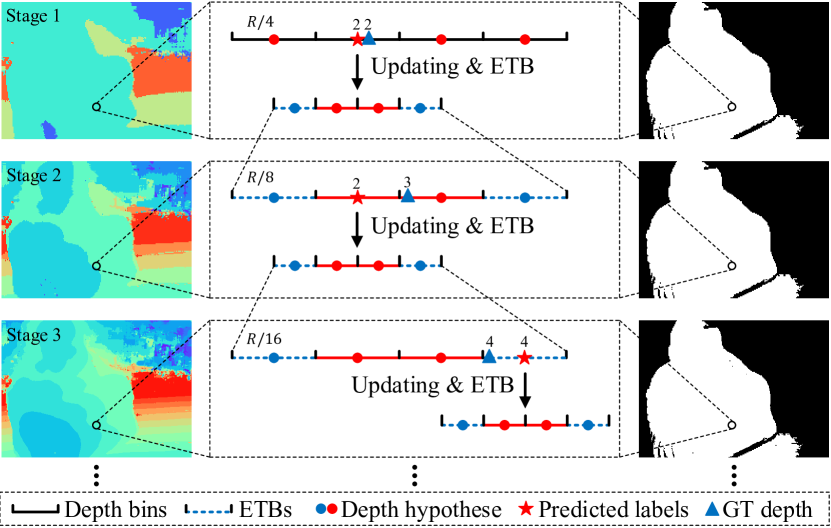
Figure 3: Illustration of Generalized Binary Search. We subdivide the selected bin into two bins according to the label. Then we pad Error Tolerance Bins (ETB) on both sides. We check the gradient mask of this pixel. Only if it is valid, the loss could participate in back-propagation.

3.4 Generalized Binary Search for MVS

To handle the error accumulation and the training issue in the proposed Binary Search for MVS, we extend it to a Generalized Binary Search for MVS. Specifically, we further design three effective mechanisms which are error tolerance bins, gradient-masked optimization and efficient gradient updating mechanism, making substantial improvement over the Binary Search method.

Error Tolerance Bins. After obtaining the selected bin $B_{k,j}$ in the $k$-th search stage, we first divide it into two new bins $B_{k+1,1}$ and $B_{k+1,2}$ for the next $(k+1)$-th stage, as shown in Fig. 3. To make the network have a certain capability of tolerating prediction errors, we propose to respectively add one small bins on the left side of $B_{k+1,1}$ and on the right side of $B_{k+1,2}$. This process is termed as Error Tolerance Bins (ETB). More formally, given $D$ ($D$ is an even number and small enough) as the final number of bins, we pad $(D-2)/2$ more bins to the two sides of the original two bins. After the padding, $D$ new bins, i.e.  $\{B_{k+1,j}|j=1,...,D\}$, are obtained, as well as their corresponding bin edges, i.e. $\{e_{k+1,m}|m=1,...,D+1\}$. We still sample the center points as the depth hypotheses $\{d_{k+1,j}|j=1,...,D\}$ from these bins with Eq. 4. The error tolerance bins extend the sampling of depth hypotheses to a range out of the two original bins in the binary search, thus enabling the network to correct the predictions and to reduce error accumulation to some extent. Since the depth hypotheses number is now $D$, we also change the initialization of depth hypotheses in the first stage. As the initial depth range $R$ in split into $D$ bins, the initial bin width is $R/D$ and in the $k$-th stage, the bin width is $R/(D\times 2^{k-1})$.

In our network implementation, we pad only 1 ETB on both sides. This leads to a depth hypothesis number of 4, i.e. $D=4$. In the experiments, we observe dramatically improved depth prediction accuracy while notably, the memory consumption can be the same level as the original binary search, as the memory is still dominated by the 2D image encoder. Fig. 3 shows a real example of our GBi-Net. The hypothesis number $D$ is set to 4. With the error tolerance bins, the network can predict a correct label of 4 when the true depth is in $B_{3,4}$ at the $3$-th search stage, while the original binary search fails.

Gradient-Masked Optimization. The proposed GBi-Net is trained in a supervised manner. The ground-truth labels are generated from the ground-truth depth map. In the $k$-th search stage, after we obtain the bins, we calculate which bin is occupied by the ground-truth depth value. Then we can convert the ground truth depth map into a ground truth occupancy volume G with one-hot encoding, which is further used for loss calculation. One problem in the iterative search is that the ground-truth depth values for some pixels may be out of the $D$ bins. In this situation, no valid labels exist and the losses cannot be computed. This is a critical problem in network optimization. The coarse-to-fine methods typically leverage a continuous regression loss, while existing MVS methods with a discrete classification loss [42] widely employ dense space discretization.

In our GBiNet, a designed mechanism to this problem is computing a mask map for each stage, based on the bins and ground-truth depth maps. If the ground-truth depth of a pixel is in the current bins, the pixel is considered as valid. Let the ground-truth depth for a pixel be $d_{gt}$ and the current bin edges be $\{e_{m}|m=1,...,D+1\}$, omitting the stage index for simplicity. Then the pixel is valid only if:

$$e_{1}\leq d_{gt}<e_{D+1}.$$ (6)

Only the loss gradients from the valid pixels are used to update the parameters in the network. The gradients from all the invalid pixels are not accumulated. With this process, we can train both Bi-Net and GBi-net successfully, as clearly confirmed by our experimental results. The gradient-masked optimization is similar to the popular self-paced learning [25], in which at the very beginning, the network only involves easy samples (i.e. easy pixels) in training, while with the optimization proceeds, the network can predict more accurate labels for hard pixels, and most pixels will eventually participate in the learning process. As can be observed in Fig. 6(c) in the experiments, a large portion of pixels falls into the the current bins in our GBi-Net.

3.5 Network Optimization

Loss Function. Our loss function is a standard cross-entropy loss that applies on the probability volume P and a ground truth occupancy volume G. A set of the valid pixels $\Omega_{\mathbf{q}}$ is first obtained by the valid mask map and then a mean loss of all valid pixels is computed as follows:

$$Loss=\sum_{\textbf{q}\in\Omega_{\mathbf{q}}}\sum_{j=1}^{D}-\textbf{G}(j,\textbf{q})\log\textbf{P}(j,\textbf{q})$$ (7)

Memory-efficient Training. MVS methods with multiple stages [11, 5] typically average the losses from all the stages and back-propagate the gradients together. Nevertheless, this training strategy consumes significant memory because of the gradients accumulation across different stages. In our GBi-Net, we train our network in a more memory-efficient way. Specifically, we compute the loss and back-propagate the gradients immediately after each stage. The gradients are not accumulated across stages, and thus the maximum memory overhead does not exceed the stage with the largest scale. To make the training with multiple stages more stable, we first set the maximum number of search stages as 2, and gradually increase it as the epoch number increases.

Figure 4: Visualization of the final and filtered depth maps.

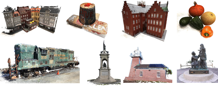
Figure 5: Point clouds examples of our method on DTU [2] and Tanks and Temples [17].

4 Experiments

4.1 Datasets

The DTU dataset [2] is an indoor dataset with multi-view images and camera poses. We Follow MVSNet [41] for dividing training and testing set. There are 27097 training samples in total. The BlendedMVS dataset [43] is a large-scale dataset with indoor and outdoor scenes. Following [45, 34, 22], we only use this dataset for training. There are 16904 training samples in total. Tanks and Temples [17] is a large-scale dataset with various outdoor scenes. It contains Intermediate subset and Advanced subset. The evaluation on this benchmark is conducted online by submitting generated point clouds to the official website.

Table 1: Point cloud evaluation results on DTU [2]. The lower is better for Accuracy (Acc.), Completeness (Comp.), and Overall. The best result is highlighted in bold and the second in italic bold. * denotes ours without using random cropping data augmentation.

Method	Acc.$\downarrow$	Comp.$\downarrow$	Overall$\downarrow$	Mem. (MB)
Tola [31]	0.342	1.190	0.766	-
Gipuma [10]	0.283	0.873	0.578	-
MVSNet [41]	0.396	0.527	0.462	9384
R-MVSNet [42]	0.383	0.452	0.417	-
CIDER [36]	0.417	0.437	0.427	-
Point-MVSNet [4]	0.342	0.411	0.376	-
CasMVSNet [11]	0.325	0.385	0.355	4591
UCS-Net [5]	0.338	0.349	0.344	4057
CVP-MVSNet [39]	0.296	0.406	0.351	-
Vis-MVSNet [45]	0.369	0.361	0.365	4775
PatchmatchNet [33]	0.427	0.277	0.352	1629
AA-RMVSNet [34]	0.376	0.339	0.357	11973
EPP-MVSNet [22]	0.413	0.296	0.355	-
Bi-Net (ours)	0.360	0.360	0.360	2108
GBi-Net* (ours)	0.327	0.268	0.298	2108
GBi-Net (ours)	0.315	0.262	0.289	2108

Table 2: Depth map evaluation results in terms of accuracy, and the memory consumption on DTU [2]. The unit of these thresholds are all in millimeters. The higher is better.

Method	$<$0.125$\uparrow$	$<$0.25$\uparrow$	$<$0.5$\uparrow$	$<$1$\uparrow$	Mem. (MB)
MVSNet [41]	8.539	16.85	32.02	53.61	9384
CasMVSNet [11]	10.13	19.88	37.04	59.4	4591
Patchmatchnet [33]	8.113	16.05	30.77	52.69	1629
GBi-Net (ours)	12.77	24.89	45.1	65.94	2108

Table 3: Point cloud evaluation results on the Advanced and Intermediate subsets of Tanks and Temples dataset [17]. Higher scores are better. The Mean is the average score of all scenes.

	Advanced							Intermediate
Method	Mean	Aud.	Bal.	Cou.	Mus.	Pal.	Tem.	Mean	Fam.	Fra.	Hor.	Lig.	M60	Pan.	Pla.	Tra.
MVSNet [41]	-	-	-	-	-	-	-	43.48	55.99	28.55	25.07	50.79	53.96	50.86	47.90	34.69
Point-MVSNet [4]	-	-	-	-	-	-	-	48.27	61.79	41.15	34.20	50.79	51.97	50.85	52.38	43.06
UCSNet [5]	-	-	-	-	-	-	-	54.83	76.09	53.16	43.03	54.00	55.60	51.49	57.38	47.89
CasMVSNet [11]	31.12	19.81	38.46	29.10	43.87	27.36	28.11	56.42	76.36	58.45	46.20	55.53	56.11	54.02	58.17	46.56
PatchmatchNet [33]	32.31	23.69	37.73	30.04	41.80	28.31	32.29	53.15	66.99	52.64	43.24	54.87	52.87	49.54	54.21	50.81
BP-MVSNet [28]	31.35	20.44	35.87	29.63	43.33	27.93	30.91	57.60	77.31	60.90	47.89	58.26	56.00	51.54	58.47	50.41
Vis-MVSNet [45]	33.78	20.79	38.77	32.45	44.20	28.73	37.70	60.03	77.40	60.23	47.07	63.44	62.21	57.28	60.54	52.07
AA-RMVSNet [34]	33.53	20.96	40.15	32.05	46.01	29.28	32.71	61.51	77.77	59.53	51.53	64.02	64.05	59.47	60.85	54.90
EPP-MVSNet [22]	35.72	21.28	39.74	35.34	49.21	30.00	38.75	61.68	77.86	60.54	52.96	62.33	61.69	60.34	62.44	55.30
Bi-Net (ours)	32.03	21.97	37.59	31.63	44.81	27.92	28.30	53.41	74.93	54.37	45.09	51.86	49.09	49.56	55.76	46.67
GBi-Net (ours)	37.32	29.77	42.12	36.30	47.69	31.11	36.93	61.42	79.77	67.69	51.81	61.25	60.37	55.87	60.67	53.89

4.2 Implementation Details

Training Details. The proposed GBi-Net is trained on the DTU dataset for DTU benchmarking and trained on BlendedMVS dataset for Tanks and Temples benchmarking, following [45, 34, 22]. We use the high-resolution DTU data provided by the open source code of MVSNet [41]. The original image size is $1200\times 1600$. We first crop the input images into $1024\times 1280$ following MVSNet [41]. Different from MVSNet [41] that directly downscale the image to $512\times 640$, we propose an online random cropping data augmentation. We randomly crop images of $512\times 640$ from images of $1024\times 1280$. The motivation is that cropping smaller images from larger images could help to learn better features for larger image scales without increasing the training overhead. When training on BlendedMVS dataset, we use the original resolution of $576\times 768$. For all the training, $N=5$ input images are used, i.e. 1 reference image and 4 source images. We adopt the robust training strategy proposed in Patchmatchnet [33] for better learning of pixel-wise weights. The maximum stage number is set to 8. For every 2 stages, we share the same feature map scale and the 3D-CNN network parameters. The whole network is optimized by Adam optimizer in Pytorch for 16 epochs with an initial learning rate of 0.0001, which is down-scaled by a factor of 2 after 10, 12, and 14 epochs. The total training batch size is 4 on two NVIDIA RTX 3090 GPUs.

Testing Details. The model trained on DTU training set is used for testing on DTU testing set. The input image number $N$ is set to 5, each with a resolution of $1152\times 1600$. It takes 0.61 seconds for each testing sample. The model trained on BlendedMVS dataset is used for testing on Tanks and Temples dataset. The image sizes are set to $1024\times 1920$ or $1024\times 2048$ to make the images divisible by 64. The input image number $N$ is set to 7. All the testings are conducted on an NVIDIA RTX 3090 GPU. We then filter and fuse depth maps of a scene into one point cloud, details in the supplemental file. Fig. 4 and Fig. 5 are visualizations of depth maps and point clouds of our method.

4.3 Benchmark Performance

Overall Evaluation on DTU Dataset. We evaluate the results on the DTU testing set by two types of metrics. The first type of metric evaluates point clouds using official evaluation scripts of DTU [2]. It compares the distance between ground-truth point clouds and the produced point clouds. The state-of-the-art comparison results are shown in Table 1. Our two models, GBi-Net and GBi-Net* both significantly improved the best performance on the completeness and the most important overall score (lower is better for both metrics). Our best model improves the overall score from 0.344 of UCSNet [5] to 0.289, while the memory is reduced by $48\%$. Note that our Bi-Net, i.e. the proposed Binary Search Network can also achieve comparable results to other dense search methods, clearly showing its effectiveness. The second type of metric directly evaluates the accuracy of the predicted depth maps. The depth ranges of DTU dataset are all 510 millimeters. Thus, we compute the depth accuracy, which counts the percentage of pixels whose absolute depth errors are less than a threshold, and 4 thresholds are considered in the evaluation (i.e. 0.125, 0.25, 0.5, 1, with millimeters as a unit). Compared to the depth range of 510 mm, these thresholds are extremely tight and challenging. The results of this type of metric are shown in Table 2. Our GBi-Net also obtains the best results on all the thresholds. The quality of depth maps also explains our best performance on point cloud evaluation.

Overall Evaluation on Tanks and Temples. We train the proposed Bi-Net and GBi-Net on BlendedMVS [43], and testing on Tanks and Temples dataset. We compare our method to state-of-the-art methods. Table 3 shows results on both the Advanced subset and the Intermediate subset. Our GBi-Net achieves the best mean score of 37.32 (higher is better) on Advanced subset compared to all the competitors, and it performs the best on 4 out of the overall 6 scenes. Note that the Advanced subset contains different large-scale outdoor scenes. The results can fully confirm the effectiveness of our method. Table 3 also shows the evaluation results on the Intermediate subset. Our GBi-Net obtains highly comparable results to the state-of-the-art. Notably, with significantly less memory, our mean score is only 0.09 lower than AA-RMVSNet [34] and 0.26 lower than EPP-MVSNet [22]. Moreover, we also obtain state-of-the-art scores on the Family and Francis scenes. Our binary search model Bi-Net also achieves satisfactory performance on both subsets. Our anonymous evaluation results on the leaderboard [1] are named as Bi-Net and GBi-Net.

Memory Efficiency Comparison. We compare the memory overhead with several previous best-performing learning-based MVS methods [41, 5, 11, 33, 44, 45, 34] on the DTU testing set. The memory usage evaluation is conducted with an image size of $1152\times 1600$. We use pytorch functions to measure the peak allocated memory usage of all the methods. Fig. 1a shows a comparison of the methods regarding memory usage and reconstruction error. Our GBi-Net shows a great improvement in the reconstruction quality while using much less memory. More specifically, the memory footprint is reduced by 77.5% compared to MVSNet [41], by 54.1% compared to CasMVSNet [11], by 82.4% to AA-RMVSNet [34], and by 55.9% to VisMVSNet [45]. Although the memory of our method is slightly $479$MB larger than Patchmatchnet [33], shown in Table 1 and 2, our method significantly outperforms it in both the point cloud (0.289 vs. 0.352) and depth map (12.77 vs. 8.113) evaluation by a large margin.

4.4 Model Analysis

Effect of Different Search Strategies. We first conduct a direct comparison on different search strategies as shown in Table 4, including dense linear search by regression (i.e. Dense LS), dense coarse-to-fine search by regression (i.e. Dense C2F), and our Bi-Net and GBi-Net search by discrete classification. In this comparison, Bi-Net and GBi-Net are trained without using the random cropping data augmentation described in Sec. 4.2. As we can observe from Table 4, our binary search networks achieve significantly better results than Dense LS and Dense C2F on both the depth performance and the memory footprint, fully confirming the effectiveness of the proposed methods.

Table 4: Performance comparison of different search strategies for MVS on DTU [2]. LS indicates linear search, and C2F indicates coarse-to-fine search. Both of them perform search via regression in a dense manner.

Method	Acc. $\downarrow$	Comp. $\downarrow$	Overall $\downarrow$	Mem (MB) $\downarrow$
Dense LS (Regression)	0.396	0.527	0.462	9384
Dense C2F (Regression)	0.325	0.385	0.355	4591
Bi-Net (Classification)	0.360	0.360	0.360	2108
GBi-Net (Classification)	0.327	0.268	0.298	2108

Effect of Stage Number. We analyze the influence of the number of search stages in our method. We test our GBi-Net model on DTU dataset with a maximum stage number of 9. We compare the reconstruction results of Stage 6, 7, 8, 9 with both the point cloud evaluation metrics and the depth map evaluation metrics. As shown in Fig.  6(a) and Fig.  6(b), the reconstruction results improve quickly from Stage 6 to 8 and then convergence, which indicates that our model can converge with a reasonably small stage number.

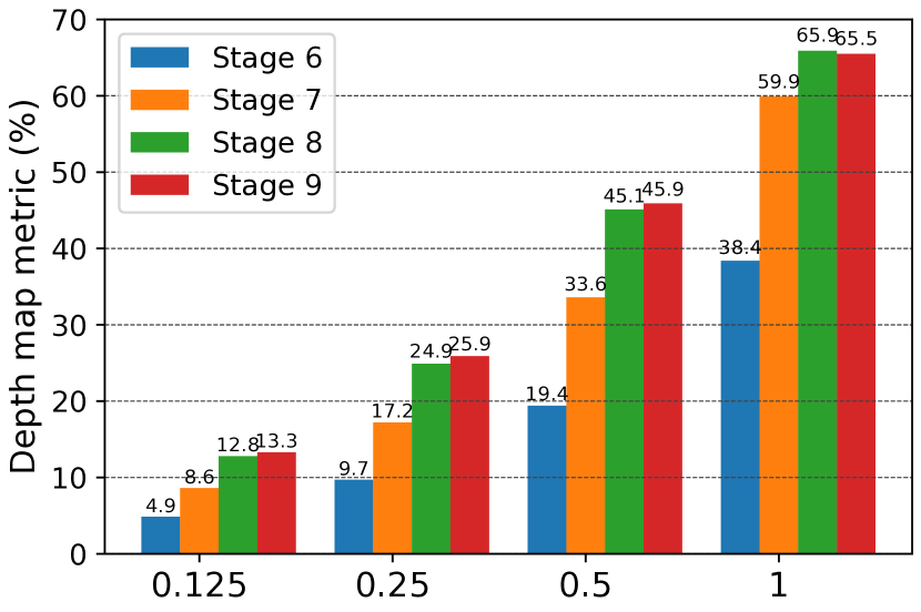
(a) Depth map evaluation

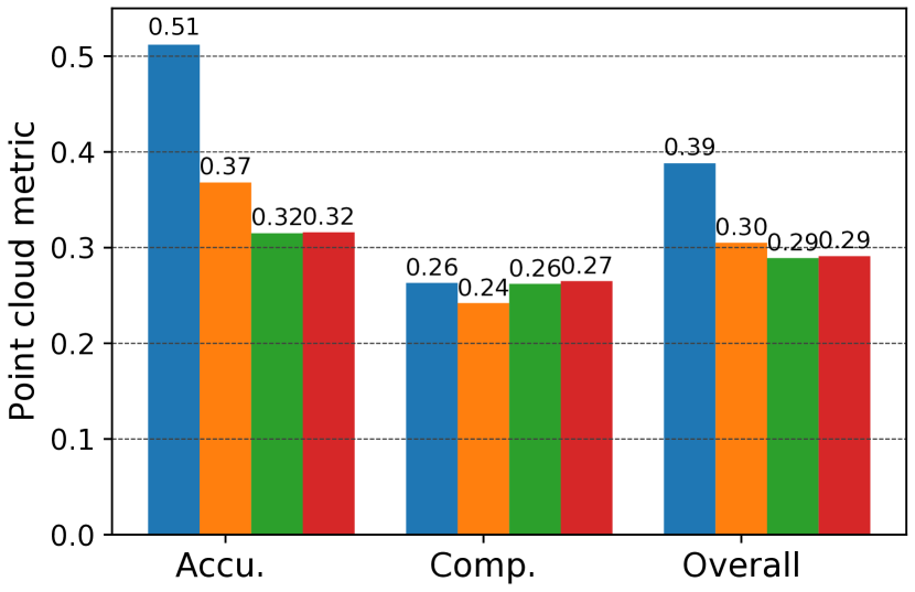
(b) Point cloud evaluation

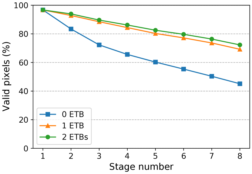
(c) Valid pixel percentage

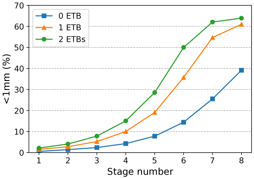
(d) $<$1mm percentage

Figure 6: (a) and (b) are evaluation results of different stage numbers. (c) and (d) are valid pixel percentage and $<$1mm percentage of different stage numbers of models with different ETBs.

Table 5: Evaluation on the number of Error Tolerance Bin (ETB), considering the performance of point cloud, depth map, and the memory usage on DTU. 0, 1 and 2 indicate respectively adding 0, 1, 2 ETBs on both sides of the search bins.

# of ETBs.	Overall $\downarrow$	$<$0.125$\uparrow$	$<$0.25$\uparrow$	$<$0.5$\uparrow$	$<$1$\uparrow$	Mem.(MB)
0	0.360	5.622	11.19	21.91	39.14	2108
1	0.298	11.75	22.92	41.62	60.99	2108
2	0.300	13.58	26.18	45.78	63.92	2438

Table 6: Point cloud evaluation and training memory overhead comparison on DTU [2] for different gradient updating strategies. GBi-Net w/GC and GBi-Net w/EGU indicate the proposed GBi-Net with commonly used gradient accumulation and the proposed efficient gradient updating, respectively.

Method	Acc.	Comp.	Overall	Memory (MB)
GBi-Net w/ GC	0.320	0.277	0.299	12137
GBi-Net w/ EGU	0.326	0.269	0.298	5208

Effect of ETB Number. We evaluate our generalized binary search with different numbers of error tolerance bins on DTU. We train 3 networks with 0, 1 and 2 ETBs on both sides, i.e. 2, 4 and 6 depth hypotheses respectively. All of the experiments run with the same setting. The evaluation results and the memory consumption are shown in Table 5. Fig. 6(c) and Fig. 6(d) also shows the valid pixel percentage and $<$1mm pixel percentage of different models in different stages. From 0 ETB to 1 ETB, we can observe a significant improvement in accuracy. This reveals the importance of ETBs. Note that the memory consumption of 1 ETB remains the same level as 0 ETB because the GPU memory is still dominated by the 2D image encoder. In Table 5, 2 ETBs model is slightly better than 1 ETB model on the depth map metric while consuming more memory. It also does not show better performance on the point cloud metric. Besides, in Fig. 6(d), the valid and $<$1mm pixel percentages of 1 ETB and 2 ETBs models are very close. All these results reveal that 1 ETB in our GBi-Net is already sufficient to achieve a good balance between accuracy and memory usage. More importantly, further increasing ETBs may make the model more complex and harder to optimize.

Effect of memory-efficient Training. We train a model without our Memory-efficient Training strategy (see Sec. 3.5) on the DTU dataset. This model averages the gradients accumulated from all the different stages and back-propagates them, which is a widely performed gradient updating scheme in existing MVS methods. As shown in Table 6, these two comparison models obtain very similar results on the depth performance, while with the proposed Memory-efficient Training, the memory consumption is largely reduced by $57.1\%$.

5 Conclusion

In this paper, we first presented a binary search network (Bi-Net) design for MVS to significantly reduce the memory footprint of 3D cost volumes. Based on this design, we further proposed a generalized binary search network (GBi-Net) containing three effective mechanisms, i.e. error tolerance bins, gradients masking, and efficient gradient updating. The GBi-Net can greatly improve the accuracy while maintaining the same memory usage as the Bi-Net. Experiments on challenging datasets also showed state-of-the-art depth prediction accuracy, and remarkable memory efficiency of the proposed methods.

Supplementary material

In this supplementary, we introduce details about the depth map fusion procedure and provide more qualitative results regarding the ablation study and the overall performance of the proposed model.

1 Depth map Fusion

As indicated in the main paper, after obtaining the final depth maps of a scene, we filter and fuse depth maps into one point cloud. The final depth maps are generated from center points of the selected bins of the final stage. We consider both the photometric and the geometric consistency for depth map filtering. The geometric consistency is similar to MVSNet [41] measuring the depth consistency among multiple views. The photometric consistency, however, is different. The probability volume P is considered to construct the photometric consistency, following R-MVSNet [42]. As the probability volume is the classification probabilities for the depth hypotheses, it measures the matching quality of these hypotheses. Since the proposed method consists of $K$ stages, we can obtain $K$ probability volumes, i.e. $\{\textbf{P}_{k}|k=1,...,K\}$. For each pixel p, its photometric consistency from its $K$ probabilities can be calculated as follows:

$$Ph(\textbf{p})=\frac{1}{K^{\prime}}\sum_{k=1}^{K^{\prime}}\max\{\textbf{P}_{k}(j,\textbf{p})|j=1,...,D\}.$$ (8)

Where $Ph(\textbf{p})$ is the photometric consistency of pixel p; $D$ is depth hypothesis number; The $\max$ operation obtains the classification probability of a selected hypothesis; $K^{\prime}$ is the maximum stage considered in photometric consistency and $1\leq K^{\prime}\leq K$. Equation 8 actually computes an average of the probabilities of the $K^{\prime}$ stages. In practice, when the maximum stage number $K=8$, we set $K^{\prime}=6$. It means that we take the average probability of the first 6 stages as the score of the photometric consistency. In our multi-stage search pipeline, as the resolutions of probability volumes are different, we upsample them to the maximum resolution of stage $K$ before the computation. After producing the photometric consistency score for each pixel, the depths of pixels are discarded if their consistency scores are below a threshold.

Figure 7a in the supplementary shows the results of each stage of a sample in the DTU dataset [2]. The depth map in each stage consists of the center-point depth values of selected bins. The quality of these depth maps can be improved quickly, demonstrating a fast search convergence of our method. The valid mask maps represent valid pixels in each search stage. Note that these mask maps are combined with the ground-truth mask maps from the dataset, and thus the background pixels are not considered. The photometric consistency (Photo. Consi.) map in stage $k$ is computed using Equation 8 by setting $K^{\prime}=k$. As shown in the Figure 7a, the photometric consistency maps is an effective measurement of depth map quality. As shown in Figure 7b, the photometric consistency (Photo. Consi.) maps from Stage 6 are used to filter the final depth maps produced from Stage 8. The filtered depth maps are further refined by geometric consistency map, and finally fused into one point cloud. Figure 8 also shows qualitative results of a sample from the Tanks and Temples [17] dataset. The background of this image is far away from the foreground and is out of the depth range, so the MVS methods predict outlier values for the background pixels. Using the photometric consistency maps, we can effectively filter out these outliers.

2 More Visualization Results

We show more qualitative results of the proposed model in this section. Figure 9 and Figure 11 show several images and their corresponding depth maps in DTU dataset [2] and Tanks and Temples dataset [17] respectively. The depth maps are filtered by photometric consistency. Figure 10 and Figure 12 shows several point clouds of our method in DTU dataset [2] and Tanks and Temples dataset [17] respectively.

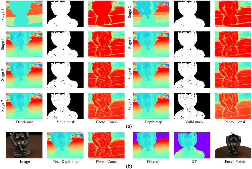
Figure 7: (a) The predicted depth maps, valid mask maps and photometric consistency (Photo. Consi.) maps in all the stages of a sample in DTU [2]. (b) The input image, final predicted depth map of Stage 8, photometric consistency (Photo. Consi.) map of Stage 6, filtered depth map by photometric consistency, ground truth depth map and fused point cloud.

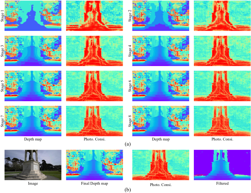
Figure 8: (a) The predicted depth maps and photometric consistency (Photo. Consi.) maps in all the stages of a sample in Tanks and Temples [17]. (b) The input image, final predicted depth map of Stage 8, photometric consistency (Photo. Consi.) map of Stage 6 and filtered depth map by photometric consistency. The background of this image is far away from the foreground and is out of the depth range so MVS methods will predicted outlier values for background pixels. With the photometric consistency, we can effectively filter out these outliers.

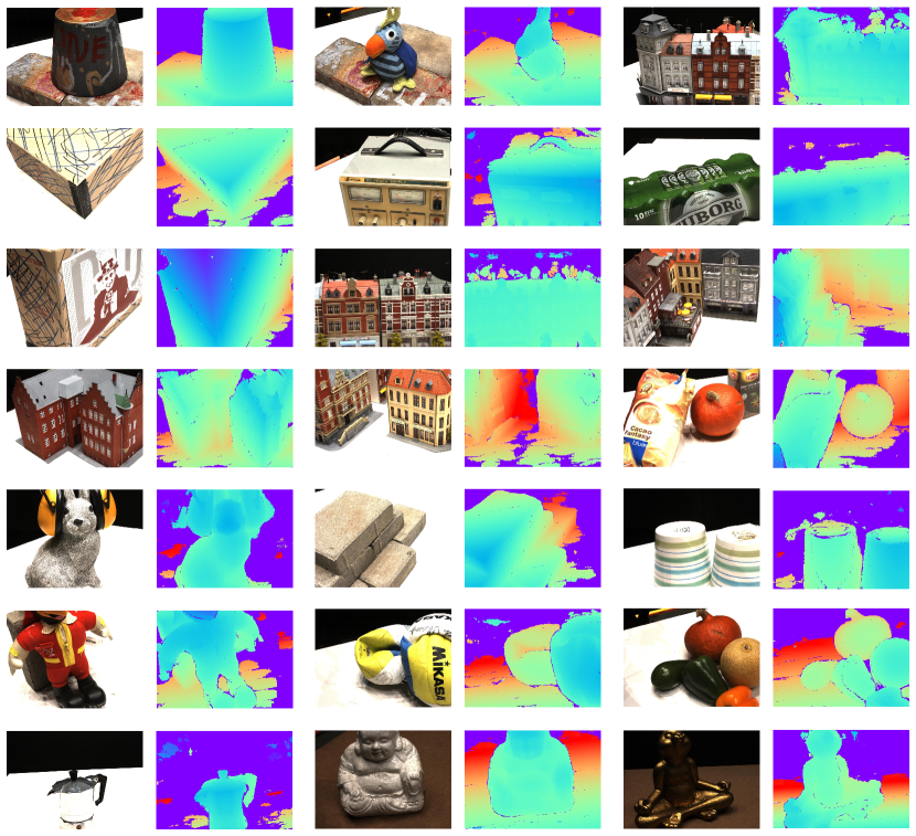
Figure 9: Examples of images and their corresponding depth maps in DTU dataset [2]. The depth maps are filtered by photometric consistency.

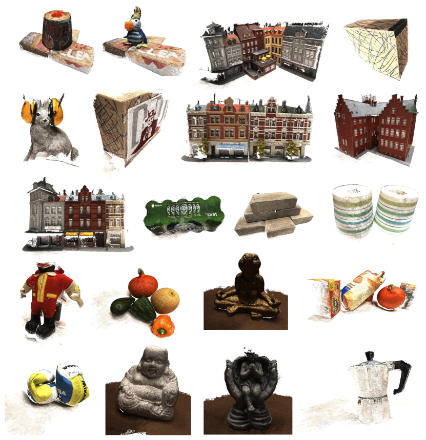
Figure 10: Point clouds of our method on DTU dataset [2].

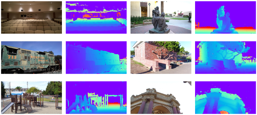
Figure 11: Examples of images and their corresponding depth maps in Tanks and Temples dataset [17]. The depth maps are filtered by photometric consistency.

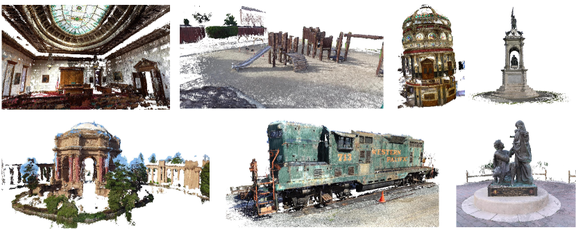
Figure 12: Point clouds of our method on Tanks and Temples dataset [17].

References

- [1] Tanks and temples leaderboard. https://www.tanksandtemples.org/leaderboard.
- [2] Henrik Aanæs, Rasmus Ramsbøl Jensen, George Vogiatzis, Engin Tola, and Anders Bjorholm Dahl. Large-scale data for multiple-view stereopsis. International Journal of Computer Vision, 120(2):153–168, 2016.
- [3] Neill DF Campbell, George Vogiatzis, Carlos Hernández, and Roberto Cipolla. Using multiple hypotheses to improve depth-maps for multi-view stereo. In ECCV. Springer, 2008.
- [4] Rui Chen, Songfang Han, Jing Xu, and Hao Su. Point-based multi-view stereo network. In ICCV, 2019.
- [5] Shuo Cheng, Zexiang Xu, Shilin Zhu, Zhuwen Li, Li Erran Li, Ravi Ramamoorthi, and Hao Su. Deep stereo using adaptive thin volume representation with uncertainty awareness. In CVPR, June 2020.
- [6] Brian Curless and Marc Levoy. A volumetric method for building complex models from range images. In Proceedings of the 23rd annual conference on Computer graphics and interactive techniques, pages 303–312, 1996.
- [7] Jifeng Dai, Haozhi Qi, Yuwen Xiong, Yi Li, Guodong Zhang, Han Hu, and Yichen Wei. Deformable convolutional networks. In ICCV, 2017.
- [8] Yasutaka Furukawa and Carlos Hernández. Multi-view stereo: A tutorial. Found. Trends. Comput. Graph. Vis., 9(1–2):1–148, June 2015.
- [9] Yasutaka Furukawa and Jean Ponce. Accurate, dense, and robust multiview stereopsis. TPAMI, 32(8):1362–1376, 2009.
- [10] Silvano Galliani, Katrin Lasinger, and Konrad Schindler. Massively parallel multiview stereopsis by surface normal diffusion. In ICCV, 2015.
- [11] Xiaodong Gu, Zhiwen Fan, Siyu Zhu, Zuozhuo Dai, Feitong Tan, and Ping Tan. Cascade cost volume for high-resolution multi-view stereo and stereo matching. In CVPR, 2020.
- [12] Xiaoyang Guo, Kai Yang, Wukui Yang, Xiaogang Wang, and Hongsheng Li. Group-wise correlation stereo network. In CVPR, 2019.
- [13] Po-Han Huang, Kevin Matzen, Johannes Kopf, Narendra Ahuja, and Jia-Bin Huang. Deepmvs: Learning multi-view stereopsis. In CVPR, June 2018.
- [14] Sunghoon Im, Hae-Gon Jeon, Stephen Lin, and In-So Kweon. Dpsnet: End-to-end deep plane sweep stereo. In ICLR, 2019.
- [15] Mengqi Ji, Juergen Gall, Haitian Zheng, Yebin Liu, and Lu Fang. Surfacenet: An end-to-end 3d neural network for multiview stereopsis. In ICCV, 2017.
- [16] Michael Kazhdan, Matthew Bolitho, and Hugues Hoppe. Poisson surface reconstruction. In Proceedings of the fourth Eurographics symposium on Geometry processing, volume 7, 2006.
- [17] Arno Knapitsch, Jaesik Park, Qian-Yi Zhou, and Vladlen Koltun. Tanks and temples: Benchmarking large-scale scene reconstruction. ACM ToG, 36(4):1–13, 2017.
- [18] Kiriakos N Kutulakos and Steven M Seitz. A theory of shape by space carving. IJCV, 38(3):199–218, 2000.
- [19] Maxime Lhuillier and Long Quan. A quasi-dense approach to surface reconstruction from uncalibrated images. TPAMI, 27(3):418–433, 2005.
- [20] Tsung-Yi Lin, Piotr Dollár, Ross Girshick, Kaiming He, Bharath Hariharan, and Serge Belongie. Feature pyramid networks for object detection. In CVPR, 2017.
- [21] Keyang Luo, Tao Guan, Lili Ju, Haipeng Huang, and Yawei Luo. P-mvsnet: Learning patch-wise matching confidence aggregation for multi-view stereo. In ICCV, 2019.
- [22] Xinjun Ma, Yue Gong, Qirui Wang, Jingwei Huang, Lei Chen, and Fan Yu. Epp-mvsnet: Epipolar-assembling based depth prediction for multi-view stereo. In ICCV, 2021.
- [23] Paul Merrell, Amir Akbarzadeh, Liang Wang, Philippos Mordohai, Jan-Michael Frahm, Ruigang Yang, David Nistér, and Marc Pollefeys. Real-time visibility-based fusion of depth maps. In ICCV, 2007.
- [24] Olaf Ronneberger, Philipp Fischer, and Thomas Brox. U-net: Convolutional networks for biomedical image segmentation. In MICCAI. Springer, 2015.
- [25] Enver Sangineto, Moin Nabi, Dubravko Culibrk, and Nicu Sebe. Self paced deep learning for weakly supervised object detection. TPAMI, 41(3):712–725, 2018.
- [26] Johannes L Schönberger, Enliang Zheng, Jan-Michael Frahm, and Marc Pollefeys. Pixelwise view selection for unstructured multi-view stereo. In ECCV. Springer, 2016.
- [27] Steven M Seitz and Charles R Dyer. Photorealistic scene reconstruction by voxel coloring. IJCV, 35(2):151–173, 1999.
- [28] Christian Sormann, Patrick Knöbelreiter, Andreas Kuhn, Mattia Rossi, Thomas Pock, and Friedrich Fraundorfer. Bp-mvsnet: Belief-propagation-layers for multi-view-stereo. In 3DV. IEEE, 2020.
- [29] Jiapeng Tang, Xiaoguang Han, Junyi Pan, Kui Jia, and Xin Tong. A skeleton-bridged deep learning approach for generating meshes of complex topologies from single rgb images. In CVPR, 2019.
- [30] Jiapeng Tang, Xiaoguang Han, Mingkui Tan, Xin Tong, and Kui Jia. Skeletonnet: A topology-preserving solution for learning mesh reconstruction of object surfaces from rgb images. TPAMI, 2021.
- [31] Engin Tola, Christoph Strecha, and Pascal Fua. Efficient large-scale multi-view stereo for ultra high-resolution image sets. Machine Vision and Applications, 23(5):903–920, 2012.
- [32] Hoang-Hiep Vu, Patrick Labatut, Jean-Philippe Pons, and Renaud Keriven. High accuracy and visibility-consistent dense multiview stereo. TPAMI, 34(5):889–901, 2011.
- [33] Fangjinhua Wang, Silvano Galliani, Christoph Vogel, Pablo Speciale, and Marc Pollefeys. Patchmatchnet: Learned multi-view patchmatch stereo. In CVPR, 2021.
- [34] Zizhuang Wei, Qingtian Zhu, Chen Min, Yisong Chen, and Guoping Wang. Aa-rmvsnet: Adaptive aggregation recurrent multi-view stereo network. In ICCV, October 2021.
- [35] Qingshan Xu and Wenbing Tao. Multi-scale geometric consistency guided multi-view stereo. In CVPR, 2019.
- [36] Qingshan Xu and Wenbing Tao. Learning inverse depth regression for multi-view stereo with correlation cost volume. In AAAI, volume 34, 2020.
- [37] Qingshan Xu and Wenbing Tao. Pvsnet: Pixelwise visibility-aware multi-view stereo network, 2020.
- [38] Jianfeng Yan, Zizhuang Wei, Hongwei Yi, Mingyu Ding, Runze Zhang, Yisong Chen, Guoping Wang, and Yu-Wing Tai. Dense hybrid recurrent multi-view stereo net with dynamic consistency checking. In ECCV, 2020.
- [39] Jiayu Yang, Wei Mao, Jose M Alvarez, and Miaomiao Liu. Cost volume pyramid based depth inference for multi-view stereo. In CVPR, 2020.
- [40] Zhenpei Yang, Zhile Ren, Qi Shan, and Qixing Huang. Mvs2d: Efficient multi-view stereo via attention-driven 2d convolutions. arXiv preprint arXiv:2104.13325, 2021.
- [41] Yao Yao, Zixin Luo, Shiwei Li, Tian Fang, and Long Quan. Mvsnet: Depth inference for unstructured multi-view stereo. In ECCV, 2018.
- [42] Yao Yao, Zixin Luo, Shiwei Li, Tianwei Shen, Tian Fang, and Long Quan. Recurrent mvsnet for high-resolution multi-view stereo depth inference. In CVPR, 2019.
- [43] Yao Yao, Zixin Luo, Shiwei Li, Jingyang Zhang, Yufan Ren, Lei Zhou, Tian Fang, and Long Quan. Blendedmvs: A large-scale dataset for generalized multi-view stereo networks. In CVPR, 2020.
- [44] Zehao Yu and Shenghua Gao. Fast-mvsnet: Sparse-to-dense multi-view stereo with learned propagation and gauss-newton refinement. In CVPR, June 2020.
- [45] Jingyang Zhang, Yao Yao, Shiwei Li, Zixin Luo, and Tian Fang. Visibility-aware multi-view stereo network, 2020.