Finite temperature QCD with physical $(u/d,s,c)$ domain-wall quarks

Abstract

In order to understand the role of QCD in the early universe, we perform hybrid Monte-Carlo simulation of lattice QCD with $N_{f}=2+1+1$ optimal domain-wall quarks at the physical point, on the $64^{3}\times(6,8,10,12,16,20,64)$ lattices, each with three lattice spacings. The lattice spacings and the bare quark masses are determined on the $64^{4}$ lattices. The resulting gauge ensembles provide a basis for studying finite temperature QCD with $N_{f}=2+1+1$ domain-wall quarks at the physical point. In this Proceeding, we present our first result on the topological susceptibility of the QCD vacuum. The topological charge of each gauge configuration is measured by the clover charge in the Wilson flow at the same flow time in physical units, and the topological susceptibility $\chi_{t}(a,T)$ is determined for each ensemble with lattice spacing $a$ and temperature $T$. Using the topological susceptibility $\chi_{t}(a,T)$ of 15 gauge ensembles with three lattice spacings and different temperatures in the range $T\sim 155-516$ MeV, we extract the topological susceptibility $\chi_{t}(T)$ in the continuum limit.

1 Introduction

The topological susceptibility $\chi_{t}$ is the most crucial quantity to measure the quantum fluctuations of the QCD vaccum. Theoretically, the topological susceptibility is defined as

$$\chi_{t}=\lim_{V\to\infty}\frac{\langle Q_{t}^{2}\rangle}{V},$$ (1)

where $Q_{t}$ is the integer-valued topological charge of the gauge field in the 4-dimensional volume $V$,

$$Q_{t}=\frac{g^{2}\epsilon_{\mu\nu\lambda\sigma}}{32\pi^{2}}\int d^{4}x\ {\rm tr}[F_{\mu\nu}(x)F_{\lambda\sigma}(x)],$$ (2)

and $F_{\mu\nu}=T^{a}F_{\mu\nu}^{a}$ is the matrix-valued field tensor, with the normalization ${\rm tr}(T^{a}T^{b})=\delta_{ab}/2$.

At zero temperature, $\chi_{t}$ is related to the chiral condensate $\Sigma$,

$$\Sigma=-\lim_{m_{q}\to 0}\lim_{V\to\infty}\frac{1}{V}\int d^{4}x\ \langle\bar{q}(x)q(x)\rangle,$$ (3)

the order parameter of the spontaneously chiral symmetry breaking, and its nonzero value gives the majority of visible (non-dark) mass in the present universe.

For QCD with $u$ and $d$ light quarks, the leading order chiral perturbation theory (ChPT) gives the relation [1]

$$\chi_{t}=\Sigma\left(\frac{1}{m_{u}}+\frac{1}{m_{d}}\right)^{-1},$$ (4)

which shows that $\chi_{t}$ is proportional to $\Sigma$. This implies that the non-trivial topological quantum fluctuations in the QCD vacuum is the origin of the spontaneously chiral symmetry breaking. In other words, if $\chi_{t}$ is zero, then $\Sigma$ is also zero and the chiral symmetry is unbroken, and the mass of the nucleon could be as light as $\sim 10$ MeV rather than $\sim 940$ MeV. Moreover, $\chi_{t}$ breaks the $U_{A}(1)$ symmetry and resolves the puzzle why the flavor-singlet $\eta^{\prime}$ is much heavier than other non-singlet (approximate) Goldstone bosons [2, 3, 4].

At temperature $T>T_{c}$, the chiral symmetry is restored and $\Sigma=0$, thus the condition for deriving (4) goes away, and the relation between $\chi_{t}$ and $\Sigma$ no longer holds. In other words, for $T>T_{c}$, $\chi_{t}$ and $\Sigma$ are independent, thus the restoration of chiral symmetry does not necessarily implies the restoration of $U_{A}(1)$ symmetry. Interestingly, the non-trivial quantum fluctuations of the QCD vacuum at $T>T_{c}$ only have the possibility to give a nonzero $\chi_{t}$ but not the $\Sigma$.

For $T>T_{c}$, $\chi_{t}(T)$ could play an important role in generating the majority of the mass in the universe, as a crucial input to the axion mass and energy density, a promising candidate for the dark matter in the universe. The axion [5, 6, 7] is a pseudo Nambu-Goldstone boson arising from the breaking of a hypothetical global chiral U(1) extension of the Standard Model at an energy scale $f_{A}$ much higher than the electroweak scale, the Pecci-Quinn mechanism. This not only solves the strong CP problem, but also provides an explanation for the dark matter in the universe. The axion mass at temperature $T$ is proportional to $\sqrt{\chi_{t}(T)}$, which is one of the key inputs to the equation of motion for the axion field evolving from the early universe to the present one, with solutions predicting the relic axion energy density, through the misalignment mechanism [8, 9, 10].

For $T<T_{c}$, the ChPT provides a prediction of $\chi_{t}(T)$ with the input $\chi_{t}(0)$ at the zero temperature [11, 12]. However, for $T>T_{c}$, the chiral symmetry is restored and the ChPT breaks down, thus the determination of $\chi_{t}(T)$ requires a non-perturbative treatment from the first principles of QCD. To this end, lattice QCD provides a viable nonperturbative determination of $\chi_{t}(T)$. Nevertheless, it becomes more and more challenging as the temperature gets higher and higher, since in principle the non-trivial configurations are more suppressed at higher temperatures, which in turn must require a much higher statatics in order to give a reliable determination. So far, direct simulations have only measured $\chi_{t}(T)$ up to $T\sim 550$ MeV.

Recent lattice studies of $\chi_{t}(T)$ aiming at the axion cosmology include various simulations with $N_{f}=0$, $2+1$, and $2+1+1$, where the lattice fermions in the unquenched simulations include the staggered fermion, the Wilson fermion, and the twisted-mass Wilson fermion [13, 14, 15, 16, 17, 18, 19]. For recent reviews, see, e.g., Refs. [20, 21] and references therein.

In this study, we perform the HMC simulation of lattice QCD with $N_{f}=2+1+1$ optimal domain-wall quarks at the physical point, on the $64^{3}\times(6,8,10,12,16,20,64)$ lattices, each with three lattice spacings $a\sim(0.064,0.068,0.075)$ fm. The bare quark masses and lattice spacings are determined on the $64^{4}$ lattices. The topological susceptibility of each gauge ensemble is measured by the Wilson flow at the flow time $t=0.8192~{}{\rm fm}^{2}$, with the clover definition for the topological charge. Using the topological susceptibility $\chi_{t}(a,T)$ of 15 gauge ensembles with 3 different lattice spacings and different temperatures in the range $T\sim 155-516$ MeV, we extract the topological susceptibility $\chi_{t}(T)$ in the continuum limit.

2 Gauge ensembles

Our present simulations with physical $(u/d,s,c)$ on the $64^{3}\times(6,8,10,12,16,20,64)\equiv N_{x}^{3}\times N_{t}$ lattices are extensions of our previous ones [22, 23, 24], using the same actions and algorithms, and the same simulation code with tunings for the computational platform Nvidia DGX-V100. Most of our production runs were performed on 10-20 units of Nvidia DGX-V100 at two institutions in Taiwan, namely, Academia Sinica Grid Computing (ASGC) and National Center for High Performance Computing (NCHC), from 2019 to 2021. Besides Nvidia DGX-V100, we also used other Nvidia GPU cards (e.g., GTX-2080Ti, GTX-1080Ti, GTX-TITAN-X, GTX-1080) for HMC simulations on the $64^{3}\times(6,8,12)$ lattices, which only require 8-22 GB device memory. We outline our HMC simulations as follows.

For the gluon fields, we use the Wilson plaquette action

$$S_{g}(U)=\beta\sum_{\text{plaq.}}\left\{1-\frac{1}{3}{\rm Re}{\rm Tr}(U_{p})\right\},$$

where $\beta=6/g_{0}^{2}$. Then setting $\beta$ to three different values $\{6.15,6.18,6.20\}$ gives three different lattice spacings. For the quark fields, we use the optimal domain-wall fermion [25] and its extension with the $R_{5}$ symmetry [26]. For domain-wall fermions, to simulate $N_{f}=2+1+1$ amounts to simulate $N_{f}=2+2+1$ since

$$\left(\frac{\det\mathcal{D}(m_{u/d})}{\det\mathcal{D}(m_{PV})}\right)^{2}\frac{\det\mathcal{D}(m_{s})}{\det\mathcal{D}(m_{PV})}\frac{\det\mathcal{D}(m_{c})}{\det\mathcal{D}(m_{PV})}=\left(\frac{\det\mathcal{D}(m_{u/d})}{\det\mathcal{D}(m_{PV})}\right)^{2}\left(\frac{\det\mathcal{D}(m_{c})}{\det\mathcal{D}(m_{PV})}\right)^{2}\frac{\det\mathcal{D}(m_{s})}{\det\mathcal{D}(m_{c})},$$ (5)

where $\mathcal{D}(m_{q})$ denotes the domain-wall fermion operator with bare quark mass $m_{q}$, and $m_{PV}$ is the Pauli-Villars mass. Since the simulation of 2-flavors is more efficient than that of one-flavor, we use the RHS of (5) for our HMC simulations. For the two-flavor factors, we use the $N_{f}=2$ pseudofermion actions [27, 28]. For the one-flavor factor, we use the exact one-flavor pseudofermion action (EOFA) for DWF [29]. The parameters of the pseudofermion actions are fixed as follows. For the $\mathcal{D}(m_{q})$ defined in Eq. (2) of Ref. [29], we fix $c=1,d=0$, $m_{0}=1.3$, $N_{s}=16$, $\lambda_{max}=6.20$, and $\lambda_{min}=0.05$. In the molecular dynamics, in order to enhance the efficiency, we use the Omelyan integrator, the Sexton-Weingarten multiple time scale method, and the mass preconditioning. The linear systems for computing the fermion forces and actions are solved by the conjugate gradient with mixed precision.

Table 1: The lattice parameters and statistics of the 15 gauge ensembles with $T>T_{c}$.

$\beta$	$a$[fm]	$N_{x}$	$N_{t}$	$T$[MeV]	$N_{\rm confs}$
6.20	0.0636	64	20	155	581
6.18	0.0685	64	16	180	650
6.20	0.0636	64	16	193	1577
6.15	0.0748	64	12	219	566
6.18	0.0685	64	12	240	500
6.20	0.0636	64	12	258	1373
6.15	0.0748	64	10	263	690
6.18	0.0685	64	10	288	665
6.20	0.0636	64	10	310	2547
6.15	0.0748	64	8	329	1581
6.18	0.0685	64	8	360	1822
6.20	0.0636	64	8	387	2665
6.15	0.0748	64	6	438	1714
6.18	0.0685	64	6	479	1983
6.20	0.0636	64	6	516	3038

The initial thermalization of each ensemble is performed in one node with 1-8 GPUs interconnected by the NVLink. After thermalization, a set of gauge configurations are sampled and distributed to 8-16 simulation units, and each unit performs an independent stream of HMC simulation. Here one simulation unit consists of 1-8 GPUs in one node, depending on the size of the device memory and the computational efficiency. Then we sample one configuration every 5 trajectories in each stream, and obtain a total number of configurations for each ensemble. The statistics of the 15 gauge ensembles with $T>T_{c}\sim 150$ MeV are listed in Table 1, where $T=1/(N_{t}a)$.

The lattice spacings and bare quark masses are determined on the $64^{4}$ lattice. For the determination of the lattice spacing, we use the Wilson flow [30, 31] with the condition

$$\left.\{t^{2}\langle E(t)\rangle\}\right|_{t=t_{0}}=0.3,$$

to obtain $\sqrt{t_{0}}/a$, then to use the input $\sqrt{t_{0}}=0.1416(8)$ fm [32] to obtain the lattice spacing $a$. The lattice spacings for $\beta=\{6.15,6.18,6.20\}$ are listed in Table 2. In all cases, the spatial volume satisfies $L^{3}>(4~{}{\rm fm})^{3}$ and $M_{\pi}L\gtrsim 3$.

Table 2: The lattice spacings and the bare quark masses of the gauge ensembles.

$\beta$	$a$[fm]	$m_{u/d}a$	$m_{s}a$	$m_{c}a$
6.15	0.0748(1)	0.00200	0.064	0.705
6.18	0.0685(1)	0.00180	0.058	0.626
6.20	0.0636(1)	0.00125	0.040	0.550

For each lattice spacing, the bare quark masses of $u/d$, $s$ and $c$ are tuned such that the lowest-lying masses of the meson operators $\{\bar{u}\gamma_{5}d,\bar{s}\gamma_{i}s,\bar{c}\gamma_{i}c\}$ are in agreement with the physical masses of $\{\pi^{\pm}(140),\phi(1020),J/\psi(3097)\}$ respectively. The bare quark masses of $u/d$, $s$, and $c$ of each lattice spacing are listed in Table 2.

To measure the chiral symmetry breaking due to finite $N_{s}=16$, we compute the residual mass according to the formula derived in Ref. [33]. The residual masses of $u/d$, $s$, and $c$ quarks are computed for each of the 15 ensembles in this study, and they are less than $1.86\%$, $0.05\%$ and $0.002\%$ of their bare masses respectively. In the units of MeV/$c^{2}$, the residual masses of $u/d$, $s$ and $c$ quarks are less than 0.09, 0.08, and 0.04 respectively. This asserts that the chiral symmetry is well preserved such that the deviation of the bare quark mass $m_{q}$ is sufficiently small in the effective 4D Dirac operator $(D_{c}+m_{q})/(1+rD_{c})$ of the optimal domain-wall fermion, for both light and heavy quarks. In other words, the chiral symmetry in our simulations should be sufficiently precise to guarantee that the hadronic observables can be determined with a good precision, with the associated uncertainty much less than those due to statistics and other systematic ones.

3 Topological charge and topological susceptibility

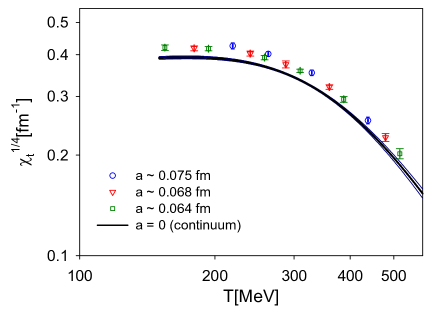
Figure 1: The fourth root of topological susceptibility $\chi_{t}^{1/4}$ versus the temperature $T$.

The topological charge $Q_{t}$ of each configuration is measured by the Wilson flow, using the clover definition. The Wilson flow equation is integrated from the flow time $t/a^{2}=0$ to 256 with the step size $0.01$. In order to extrapolate the topological susceptibility $\chi_{t}=\langle Q_{t}^{2}\rangle/V$ to the continuum limit, $Q_{t}$ is required to be measured at the same physical flow time for each configuration, which is chosen to be $0.8192~{}{\rm fm}^{2}$ such that $\chi_{t}$ attains a plateau for each ensemble in this study.

The results of $\chi_{t}^{1/4}(a,T)$ of 15 gauge ensembles are plotted in Fig. 1, which are denoted by blue circles ($a\sim 0.075$ fm), red inverted triangles ($a\sim 0.068$ fm), and green squares ($a\sim 0.064$ fm). First, we observe that the 5 data points of $\chi_{t}^{1/4}$ at high temperature $T>350$ MeV can be fitted by the power law $\chi_{t}^{1/4}(T)\sim T^{-p}$, independent of the lattice spacing $a$. However, the power law cannot fit all 15 data points. In order to construct an analytic formula which can fit all data points of $\chi_{t}(T)$ for all temperatures, one considers a function which behaves like the power law $\sim(T_{c}/T)^{p}$ for $T\gg T_{c}$, but in general it incorporates all higher order corrections, i.e.,

$$\chi_{t}^{1/4}(T)=c_{0}(T_{c}/T)^{p}\left[1+b_{1}(T_{c}/T)+b_{2}(T_{c}/T)^{2}+\cdot+b_{n}(T_{c}/T)^{n}+\cdots\right].$$ (6)

In practice, it is vital to recast (6) into a formula with fewer parameters, e.g.,

$$\chi_{t}^{1/4}(T)=c_{0}\frac{(T_{c}/T)^{p}}{1+b_{1}(T_{c}/T)+b_{2}(T_{c}/T)^{2}}.$$ (7)

It turns out that the 6 data points of $\chi_{t}^{1/4}$ at $a\sim 0.064$ fm ($\beta=6.20$) are well fitted by (7). Thus, for the global fitting of all $\chi_{t}^{1/4}(a,T)$ with different $a$ and $T$, the simplest extension of (7) is to replace $c_{0}$ with $(c_{0}+c_{1}a^{2})$. This leads to the ansatz

$$\chi_{t}^{1/4}(a,T)=(c_{0}+c_{1}a^{2})\frac{(T_{c}/T)^{p}}{1+b_{1}(T_{c}/T)+b_{2}(T_{c}/T)^{2}},\hskip 11.38109ptT_{c}=150~{}{\rm MeV}.$$ (8)

Fitting the 15 data points of $\chi_{t}^{1/4}$ in Fig. 1 to (8), it gives $c_{0}=1.89(3)$, $c_{1}=32.2(6.8)$, $p=2.03(5)$, $b_{1}=-2.42(19)$, $b_{2}=6.25(14)$ with $\chi^{2}$/d.o.f. = 0.21. Note that the fitted value of the exponent $p$ is rather insensitive to the choice of $T_{c}=150~{}{\rm MeV}$, i.e., any value of $T_{c}$ in the range of 145-155 MeV gives almost the same value of $p$. Then $\chi_{t}^{1/4}(T)$ in the continuum limit can be obtained by setting $a^{2}=0$ in (8), which is plotted as the solid black line in Fig. 1, with the error bars as the enveloping blue solid lines. In the limit $T\gg T_{c}$, it becomes $\chi_{t}^{1/4}(T)=c_{0}(T_{c}/T)^{2.03(5)}$, i.e., $\chi_{t}(T)=c_{0}^{4}(T_{c}/T)^{8.1(2)}$, which agrees with the temperature dependence of $\chi_{t}(T)$ in the dilute instanton gas approximation (DIGA) [34], i.e., $\chi_{t}(T)\sim T^{-8.3}$ for $N_{f}=4$. This also implies that our data points of $\chi_{t}(a,T)$ (for $T>350$ MeV) are valid, up to an overall constant factor.

It is interesting to note that our 15 data points of $\chi_{t}(a,T)$ are only up to the temperature $T\sim 515$ MeV. Nevertheless, they are sufficient to fix the coefficents of (8), which in turn can give $\chi_{t}(T)$ for any $T>T_{c}$. This is the major advantage of having an analytic formula like (8). There are many possible variations of (8), e.g., replacing $(c_{0}+c_{1}a^{2})$ with $(c_{0}+c_{1}a^{2}+c_{2}a^{4})$, adding the $a^{2}$ term to the exponent $p$ and/or the coefficients $b_{1}$ and $b_{2}$, etc. For our 15 data points, all variations give consistent results of $\chi_{t}(T)$ in the continuum limit.

4 Discussions

To summarize, this is the first determination of $\chi_{t}(T)$ in lattice QCD with $N_{f}=2+1+1$ optimal domain-wall quarks at the physical point, by direct simulations. Here the chiral symmetry is preserved with $N_{s}=16$ in the fifth dimension, and the optimal weights $\{\omega_{s},s=1,\cdots,16\}$ are computed with $\lambda_{min}=0.05$ and $\lambda_{max}=6.2$, and the error of the sign function of $H_{w}$ is less than $1.2\times 10^{-5}$, for eigenvalues of $H_{w}$ satisfying $\lambda_{min}\leq|\lambda(H_{w})|\leq\lambda_{max}$. However, it is not in the exact chiral symmetry limit, the smallest eigenvalue of the effective 4D Dirac operator $D(m_{q})=(D_{c}+m_{q})/(1+rD_{c})$ is larger than $m_{q}$. Thus the fermion determinant is larger than its value in the exact chiral symmetry limit. Now the question is how $\chi_{t}(T)$ depends on the chiral symmetry in this study. For optimal domain-wall fermion, the exact chiral symmetry is in the limit $N_{s}\to\infty$ and $\lambda_{min}\to 0$. In practice, this can be attained by increasing $N_{s}$ and decreasing $\lambda_{min}$ such that the error due to the chiral symmetry breaking becomes negligible in any physical observables. For example, if one takes $N_{s}=32$, $\lambda_{min}=10^{-4}$ and $\lambda_{max}=6.2$, then the error of the sign function of $H_{w}$ is less than $1.2\times 10^{-5}$ for eigenvalues of $H_{w}$ satisfying $10^{-4}\leq|\lambda(H_{w})|\leq 6.2$. Nevertheless, this set of simulations is estimated to be $\sim 100$ times more expensive than the present one, beyond the limit of our present resources. At this point, one may wonder whether it is possible to use the reweighting method to obtain $\chi_{t}(a,T)$ in the exact chiral symmetry limit, without performing new simulations at all. However, according to our discussion of the reweighting method for DWF [35], it is infeasible to apply the reweighting method to the $\chi_{t}(a,T)$ results in the present study, thus new simulations with smaller $\lambda_{min}$ and larger $N_{s}$ are required.

References

- [1] H. Leutwyler and A. V. Smilga, Phys. Rev. D 46, 5607-5632 (1992)
- [2] G. ’t Hooft, Phys. Rev. Lett. 37, 8-11 (1976); Phys. Rev. D 14, 3432-3450 (1976) [erratum: Phys. Rev. D 18, 2199 (1978)]
- [3] E. Witten, Nucl. Phys. B 156, 269-283 (1979)
- [4] G. Veneziano, Nucl. Phys. B 159, 213-224 (1979)
- [5] R. D. Peccei and H. R. Quinn, Phys. Rev. Lett. 38, 1440-1443 (1977); Phys. Rev. D 16, 1791-1797 (1977)
- [6] S. Weinberg, Phys. Rev. Lett. 40, 223-226 (1978)
- [7] F. Wilczek, Phys. Rev. Lett. 40, 279-282 (1978)
- [8] M. Dine, W. Fischler and M. Srednicki, Phys. Lett. B 104, 199-202 (1981)
- [9] J. Preskill, M. B. Wise and F. Wilczek, Phys. Lett. B 120, 127-132 (1983)
- [10] L. F. Abbott and P. Sikivie, Phys. Lett. B 120, 133-136 (1983)
- [11] J. Gasser and H. Leutwyler, Phys. Lett. B 184, 83-88 (1987)
- [12] F. C. Hansen and H. Leutwyler, Nucl. Phys. B 350, 201-227 (1991)
- [13] E. Berkowitz, M. I. Buchoff and E. Rinaldi, Phys. Rev. D 92, no.3, 034507 (2015) [arXiv:1505.07455 [hep-ph]].
- [14] R. Kitano and N. Yamada, JHEP 10, 136 (2015) [arXiv:1506.00370 [hep-ph]].
- [15] S. Borsanyi, M. Dierigl, Z. Fodor, S. D. Katz, S. W. Mages, D. Nogradi, J. Redondo, A. Ringwald and K. K. Szabo, Phys. Lett. B 752, 175-181 (2016) [arXiv:1508.06917 [hep-lat]].
- [16] C. Bonati, M. D’Elia, M. Mariti, G. Martinelli, M. Mesiti, F. Negro, F. Sanfilippo and G. Villadoro, JHEP 03, 155 (2016) [arXiv:1512.06746 [hep-lat]].
- [17] P. Petreczky, H. P. Schadler and S. Sharma, Phys. Lett. B 762, 498-505 (2016) [arXiv:1606.03145 [hep-lat]].
- [18] S. Borsanyi, Z. Fodor, J. Guenther, K. H. Kampert, S. D. Katz, T. Kawanai, T. G. Kovacs, S. W. Mages, A. Pasztor and F. Pittler, et al. Nature 539, no.7627, 69-71 (2016) [arXiv:1606.07494 [hep-lat]].
- [19] F. Burger, E. M. Ilgenfritz, M. P. Lombardo and A. Trunin, Phys. Rev. D 98, no.9, 094501 (2018) [arXiv:1805.06001 [hep-lat]].
- [20] G. D. Moore, EPJ Web Conf. 175, 01009 (2018) [arXiv:1709.09466 [hep-ph]].
- [21] M. P. Lombardo and A. Trunin, Int. J. Mod. Phys. A 35, no.20, 2030010 (2020) [arXiv:2005.06547 [hep-lat]].
- [22] Y. C. Chen and T. W. Chiu [TWQCD Collaboration], Phys. Lett. B 767, 193 (2017) [arXiv:1701.02581 [hep-lat]].
- [23] T. W. Chiu [TWQCD Collaboration], PoS LATTICE2018, 040 (2018) [arXiv:1811.08095 [hep-lat]].
- [24] T. W. Chiu [TWQCD Collaboration], PoS LATTICE2019, 133 (2020) [arXiv:2002.06126 [hep-lat]].
- [25] T. W. Chiu, Phys. Rev. Lett. 90, 071601 (2003) [hep-lat/0209153]
- [26] T. W. Chiu, Phys. Lett. B 744, 95 (2015) [arXiv:1503.01750 [hep-lat]].
- [27] T. W. Chiu, T. H. Hsieh, Y. Y. Mao [TWQCD Collaboration], Phys. Lett. B 717, 420 (2012) [arXiv:1109.3675 [hep-lat]].
- [28] Y. C. Chen and T. W. Chiu, Phys. Rev. D 100, no.5, 054513 (2019) [arXiv:1907.03212 [hep-lat]].
- [29] Y. C. Chen and T. W. Chiu [TWQCD Collaboration], Phys. Lett. B 738, 55 (2014) [arXiv:1403.1683 [hep-lat]].
- [30] R. Narayanan and H. Neuberger, JHEP 0603, 064 (2006) [hep-th/0601210].
- [31] M. Luscher, JHEP 1008, 071 (2010) Erratum: [JHEP 1403, 092 (2014)] [arXiv:1006.4518 [hep-lat]].
- [32] A. Bazavov et al. [MILC Collaboration], Phys. Rev. D 93, no. 9, 094510 (2016) [arXiv:1503.02769 [hep-lat]].
- [33] Y. C. Chen, T. W. Chiu [TWQCD Collaboration], Phys. Rev. D 86, 094508 (2012) [arXiv:1205.6151 [hep-lat]].
- [34] D. J. Gross, R. D. Pisarski and L. G. Yaffe, Rev. Mod. Phys. 53, 43 (1981)
- [35] Y. C. Chen, T. W. Chiu and T. H. Hsieh, [arXiv:2204.01556 [hep-lat]].