Hydrodynamics and transport
in the long-range-interacting $\varphi^{4}$ chain

Abstract

We present a simulation study of the one-dimensional $\varphi^{4}$ lattice theory with long-range interactions decaying as an inverse power $r^{-(1+\sigma)}$ of the intersite distance $r$, $\sigma>0$. We consider the cases of single and double-well local potentials with both attractive and repulsive couplings. The double-well, attractive case displays a phase transition for $0<\sigma\leq 1$ analogous to the Ising model with long-range ferromagnetic interactions. A dynamical scaling analysis of both energy structure factors and excess energy correlations shows that the effective hydrodynamics is diffusive for $\sigma>1$ and anomalous for $0<\sigma<1$ where fluctuations propagate superdiffusively. We argue that this is accounted for by a fractional diffusion process and we compare the results with an effective model of energy transport based on Lévy flights. Remarkably, this result is fairly insensitive on the phase transition. Nonequilibrium simulations with an applied thermal gradient are in quantitative agreement with the above scenario.

Keywords: Transport processes / heat transfer (Theory), Fluctuating hydrodynamics, Long-range interactions

1 Introduction

Nonequilibrium properties of many-body statistical systems on macroscopic scales are usually well described by hydrodynamic equations. This is justified by the fact that macroscopic fluctuations of conserved quantities (and order parameters close to criticality) must evolve slowly with respect to microscopic time-scales to reach a steady state. If the relevant correlations have long-time tails, standard diffusive behavior may break down as it happens generically in nonlinear, low-dimensional systems [1, 2, 3, 4]. Anomalous transport in such many-body systems can be effectively described by a random Lévy walk [5] of the energy carriers, as demonstrated extensively in the literature [6, 7, 8]. This leads naturally to consider hydrodynamic equations where the standard Laplacian operator is replaced by a fractional one [9, 10, 11, 12]. Nonlinear coupling among hydrodynamic fields yields slow algebraic decay of current correlations at equilibrium and effective non-local equations. A theoretical justification of such a behavior has been obtained by the nonlinear fluctuating hydrodynamics approach, whereby long-wavelength fluctuations are described in terms of the Kardar-Parisi-Zhang equations [13]. Although the resulting predictions are well confirmed by numerical simulations [14, 15, 16], there may be significant scale-effects, especially when the dynamics is only weakly chaotic [17].

In presence of long-range forces one may expect non-local effective hydrodynamic description to arise naturally by the non-local nature of couplings. Indeed, perturbations may propagate with infinite velocities, making this class of systems qualitatively different from their short-ranged counterparts [18, 19]. This has also effects on energy transport for open systems interacting with external reservoirs and, more generally, on the way in which the long-range terms couple the system with the environment. For nonlinear oscillator assemblies this problem has received some attention in the recent literature [20, 21, 22, 23, 24, 25] but is less developed with respect to the short-range case. A further complication is that relaxation to local and global equilibrium may occur through long-living metastable states and exhibit anomalous diffusion of energy [26, 27, 28] and even lack of thermalization upon interaction with a single external bath [29].

Another motivation of the present study is to understand the role of phase transitions on anomalous transport in low-dimensional systems. As it is known, there is a well-established theory of dynamical critical phenomena [30] which gives insight on transport coefficients at criticality. However, studies of energy transport in microscopic models are scarce, mostly limited to spin systems see e.g. [31, 32, 33] for some related results on critical Ising models with nearest-neighbor coupling.

Besides the above theoretical motivations, the physics of long-range interacting oscillator arrays has interesting experimental applications. The most natural candidates are trapped ion chains, where ions can be confined in periodic arrays and can be studied in an open setup [34, 35]. Quantum spins with tunable long-range interactions can be realized in the laboratory and the propagation of a disturbance can be studied [36]. On a macroscale, effective long-range forces arise for tailored macroscopic systems like chain of coupled magnets [37] and the effects of fluctuations and nonlinearity may be relevant. Several other application have been considered, and we refer to [38] for a recent account.

In this paper, we study the hydrodynamic properties of a one-dimensional chain of single or double-well oscillators interacting through a long-range potential that can be either attractive or repulsive. It can be seen as a discretization of a $\varphi^{4}$ field theory, directly related to the long-range Ising model and, thus, an effective description of spin chains with coupling decaying as an inverse power of their relative distance [36]. The paper is organized as follows. In Section 2 we define the model and discuss its general properties. In Section 3 we present the results obtained from equilibrium simulations concerning the dynamical scaling analysis of structure factors and of excess energy correlations. The single-well potential and the double-well case are separately analyzed. In Section 4 we introduce an effective stochastic model of long-range transport based on a Lévy flight process and we show that it can reproduce the dynamical scaling observed in the $\varphi^{4}$ lattice. Stationary out-of-equilibrium states resulting from application of suitable thermal imbalances and the corresponding scaling of heat fluxes are also analyzed. Steady nonequilibrium states of the $\varphi^{4}$ model are presented separately in Section 5 along with a discussion of finite-size effects. Finally, Sections 6 and 7 are respectively devoted to a discussion of the results and to some concluding remarks.

2 The long-range-interacting $\varphi^{4}$ lattice in one dimension

We consider a one-dimensional lattice of $N$ particles with periodic boundary conditions, whose dynamics is governed by the long-range Hamiltonian

$$H=\sum_{i=1}^{N}\left[\frac{p_{i}^{2}}{2}+U(q_{i})-\frac{\mu}{\mathcal{N}_{\sigma}}\sum_{j>i}^{N}\,\frac{q_{i}q_{j}}{d_{ij}^{1+\sigma}}\right]$$ (1)

where $\mu$ is a coupling constant. The $q_{i}$s are continuous real variables that denote the oscillator displacements while $p_{i}=\dot{q}_{i}$ are the corresponding momenta (we set all the masses to unity henceforth). The cases $\mu>0$ and $\mu<0$ correspond to ferromagnetic (attractive) and antiferromagnetic (repulsive) interactions, respectively. The quantity $d_{ij}$ identifies the shortest distance between sites $i$ and $j$ on a periodic lattice

$$d_{ij}=\min\{|i-j|,N-|i-j|\}.$$ (2)

The real exponent $\sigma\geq-1$ is the parameter that controls the interaction range. The case $\sigma=0$ identifies the extensivity threshold in one dimension [27]. We follow the usual Kac prescription to keep the potential energy extensive even when $\sigma<0$, by defining

$${\mathcal{N}}_{\sigma}=2\sum_{r=1}^{N/2}\frac{1}{r^{1+\sigma}}.$$ (3)

Notice that for $\sigma=-1$, i.e. the case of a mean-field interaction, $N_{-1}=N$. For $\sigma>0$ ${\mathcal{N}}_{\sigma}$ attains a constant value for large sizes $N$ and diverges for $\sigma<0$. Finally, in the limit of $\sigma\to+\infty$ the case of nearest-neighbor interactions is retrieved. In the present work we will concentrate on the weak-long range case, $\sigma>0$.

For generic choices of the local potential $U(q)$ the model is nonintegrable, with the energy being the only constant of motion. We consider here the $\varphi^{4}$ potential [39]

$$U(q)=\pm\frac{q^{2}}{2}+\frac{q^{4}}{4};$$ (4)

in suitable units. Let us first discuss the attractive coupling $\mu>0$. The single-well case, $+1$ in (4), identifies the long-range generalization of the non-linearly pinned chain (or discrete Klein-Gordon field). The ground state corresponds to all particles at rest with $q_{i}=0$ and the model is expected to admit only a disordered (paramagnetic) phase. Transport properties in the nearest-neighbor case have been thoroughly studied in the past [40, 41, 42]. Generically, energy fluctuations diffuse normally, following the standard heat equation with a finite thermal diffusivity in the thermodynamic limit.

The double well case, $-1$ in (4), is of particular interest and indeed its nearest-neighbor version has been considered starting from the seventies of last century [43]. It can be can be seen as a Hamiltonian, lattice version of the familiar $\varphi^{4}$ scalar field with long-range forces. The model has two degenerate ground states with $q_{n}=g$ and $g=\pm\sqrt{\mu+1}$, corresponding to an energy density $e=H/N=-(\mu+1)^{2}/4$ independently on $\sigma$ (notice that the ground state displacement $g$ does not coincide with the minima of $U(q)$, which are equal to $\pm 1$). Since the model has the same symmetries of the ferromagnetic Ising model with long-range couplings [44], its equilibrium critical properties should be in the same universality class. Indeed, one can think of the $q_{i}$s as a coarse-grained version of the Ising spins. It is thus natural to consider as order parameter the average of the “magnetization” density

$$m=\frac{1}{N}\sum_{i=1}^{N}q_{i}$$

Remarkably, depending on $\sigma$ the double-well chain can display a phase transition in the weak-long range regime. This can be justified as follows. Following [45], for weak long range interactions in $d$ dimensions one can write a Landau-Ginzburg effective free energy of the form

$$F_{GL}=\int d^{d}r\left[\frac{1}{2}a_{2}m^{2}({\bf r})+\frac{1}{4}a_{4}m^{4}({\bf r})\right]+\int d^{d}r~{}d^{d}r^{\prime}\frac{m({\bf r})m({\bf r^{\prime}})}{|{\bf r-r^{\prime}}|^{d+\sigma}}~{},$$ (5)

where $a_{2}$, $a_{4}$ are suitable coefficients and $m(\bf r)$ is the magnetization field at point ${\bf r}\in\mathbb{R}^{d}$. The second term represents the contribution of the long-range forces to the energy. In terms of the Fourier components of the order parameter $m({\bf k})=\int d^{d}r\,m({\bf r})e^{i{\bf k}\cdot\bf r}$ this integral may be expressed as a Gaussian approximation (far from criticality). Accordingly, to leading order in $k$, the Fourier transform of the long range potential is of the form $a+bk^{\sigma}$, where $a$ and $b$ are constants. Therefore one obtains

$$F_{GL}=\frac{1}{2V}\sum_{{\bf k}}(\bar{a}_{2}+bk^{\sigma}+k^{2})m({\bf k})m(-{{\bf k}})~{},$$ (6)

where $\bar{a}_{2}=a_{2}+a$. The $k^{2}$ term results from short range interactions which are always present in the system. For $\sigma>2$ the $k^{\sigma}$ term in (6) is dominated by the $k^{2}$ term in the long-wavelength limit and may thus be neglected. One is then back to the model corresponding to short range interactions and the upper critical dimension is $d_{c}=4$. On the other hand, for $0<\sigma<2$ the term is $k^{\sigma}$ dominates and the correlation length diverges as $\xi\propto|\bar{a}_{2}|^{-1/\sigma}$ [45].

This expectation has been demonstrated numerically and analytically for the mean-field case $\sigma=-1$ both in the canonical [46] and microcanonical [47] ensembles. In the range $0<\sigma<1$, the transition is of second order, separating a ferromagnetic phase at low temperatures from a paramagnetic phase at high temperatures. For $\sigma>1$, the system is disordered at all energies. The case $\sigma=1$ is peculiar, since it shows a Kosterlitz-Thouless phase transition with a discontinuous jump in the magnetization [48]. For $1<\sigma<d/2$ the transition is mean-field with exponents independent on $\sigma$, while for $d/2<\sigma<1$ they depend continuously on $\sigma$ [45]. We refer also to [39] for further studies of critical properties of the model .

The antiferromagnetic, repulsive case $\mu<0$ has been studied in the mean-field limit $\sigma=-1$, where it was shown that no phase transition occurs in this limit [47]. To our knowledge, the case $\sigma>-1$ has not been studied so far. Based again on the analogy with the antiferromagnetic Ising model with long-range interaction [49] we do not expect any phase transition here.

In the following Section we will present some numerical results that confirm the above expectations.

3 Equilibrium simulations

In this Section we report the results of equilibrium microcanonical simulations of the model. Numerical integration of the associated Hamilton equations can be computationally demanding in long-range interacting systems. However, since the distance $d_{ij}$ only depends on $|i-j|$, it turns out that the matrix of coupling strengths among oscillators, namely $d_{ij}^{-1}$, is circulant. One can thus exploit translational invariance to compute the forces as convolution products by an algorithm based on the Fast Fourier Transform [50]. The simulation protocol to sample an equilibrium configuration for a given temperature $T$ is the following.

• For the double-well local potential, canonical variables are initialized as $q_{n}(0)=\pm 1$ with equal probability and $p_{n}(0)$ randomly drawn from a Gaussian distribution with width $\sqrt{T}$. For the single-well potential, initial displacements are chosen as $q_{n}(0)=0$;

• The system is let evolve for a canonical transient whereby a subset of randomly chosen particles (typically $5\%$) undergo random collisions with a Maxwellian bath at temperature $T$. Each collision event amounts to assign to the colliding particle a new velocity $p_{n}=v$, with $v$ being a random Gaussian with width $\sqrt{T}$. This allows to thermalize the initial configuration and fix the energy density $e=H/N$ corresponding to the desired temperature;

• Finally, Maxwellian collisions are switched off and a microcanonical trajectory is generated by means of a 4th-order symplectic algorithm [51]. Statistical averages of the relevant observables, as the kinetic temperature $T=\langle p_{i}^{2}\rangle$, are thereby computed.

For the sake of illustration, we report in fig.1 the magnetization and caloric curves for different lattice sizes, as obtained by microcanonical simulation of the double-well ferromagnetic ($\mu>0$) model. Up to the statistical fluctuations and finite-size effects, a continuous transition in $m(e)$ at a critical energy density $e_{c}$ is clearly seen, along with a discontinuos change of the slope of the caloric curve $T(e)$ at $T_{c}=T(e_{c})$. The difference between the two phases can be seen by computing the equilibrium probability distribution of the $q_{i}$’s (data not shown). In the sub-critical phase $T<T_{c}$ this distribution is asymmetric with a main peak in correspondence of one of the two degenerate ground states, while it is symmetric in the disordered phase $T>T_{c}$, as expected. To quantify the strength of the nonlinear term we also report in figure 1(b) the ratio $R=\langle H_{4}\rangle/\langle H_{2}\rangle$ where $H_{2}$ and $H_{4}$ are, respectively, the quadratic and quartic parts of the Hamiltonian (1). Since $R$ is of order one in the considered energy regimes, this clearly confirms that we are very far from the weakly-nonlinear case.

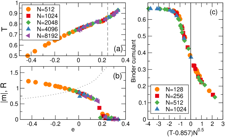
Figure 1: Illustrating the second-order phase transition in the double-well model, $\mu=1$, $\sigma=0.6$, microcanonical simulation as described in the main text: (a) caloric curves for different lattice sizes and (b) absolute value of the magnetization (symbols); the dotted line is the ratio $R$ between the average of the anharmonic and harmonic energies (see text). Panel (c) illustrates the finite-size scaling analysis of the Binder cumulant $B$ as a function of the scaled temperature $(T-T_{c})N^{0.5}$. $T_{c}$ is estimated by looking for the intersection point of the curves $B(T,N)$. The vertical line in (a) signals the best estimate of the critical energy $e_{c}\approx 0.249$ corresponding to $T_{c}\approx 0.857$.

To locate the critical point we used the well-known finite-size scaling method, (see e.g. [52] and references therein for application to the short-ranged $\varphi^{4}$ lattice). We computed the Binder cumulant $B(T,N)=1-\langle m^{4}\rangle/3\langle m^{2}\rangle^{2}$ for different lattice sizes. Following the standard prescription this alllows to estimate the critical kinetic temperature $T_{c}$, as shown in fig.1c. The accuracy of such estimates are sufficient for our purposes and we did not attempt to measure critical exponents.

We also performed some simulations for the double-well model with repulsive interaction, setting $\mu=-1$. For the explored cases, the average magnetization $\langle m\rangle$ is vanishingly small and the caloric curves do not display any sign of discontinuities. This confirm the expectation that the repulsive model is not critical.

Since we are interested in large scale (hydrodynamic) properties, we investigated equilibrium correlation functions in the long-time and distance regime. As it is known, this gives direct information on propagating modes on such scales. In heat transport problems one is primarily interested in the propagation of energy fluctuations. We thus consider the site energies

$$h_{i}=\frac{p_{i}^{2}}{2}+U(q_{i})-\frac{\mu}{{\mathcal{N}}_{\sigma}}\sum_{j\neq i}^{N}\,\frac{q_{i}q_{j}}{d_{ij}^{1+\sigma}},$$ (7)

which are inherently non-local. Moreover, despite our study is focused on energy transport ad relaxation, in the following we will also report some correlation data of the $q_{n}$, namely of the local magnetization.

For computational reasons it is convenient to work in the Fourier domain, i.e. we first perform the discrete transform

$$h(k,t)={1\over N}\,\sum_{n=1}^{N}\,h_{n}\exp(-ikn),\quad m(k,t)={1\over N}\,\sum_{n=1}^{N}\,q_{n}\exp(-ikn)$$ (8)

By virtue of the periodic boundaries, the allowed values of the wavenumber $k$ are integer multiples of $2\pi/N$. We then define the dynamical structure factors, namely the square modulus of the temporal Fourier transform, as

$$S_{h}(k,\omega)\;=\;\big{\langle}\big{|}h(k,\omega)\big{|}^{2}\big{\rangle},\quad S_{m}(k,\omega)\;=\;\big{\langle}\big{|}m(k,\omega)\big{|}^{2}\big{\rangle}\quad.$$ (9)

The square brackets denote an average over a set of independent molecular–dynamics runs (typically a few hundreds). Simulations have been performed for a relatively large lattice size $N=2048$. In some case a check of finite-size effect has been done by comparing the structure factors (at fixed $k$) for $N=4096$.

A complementary approach is to compute the spatio-temporal correlations, that are useful to ascertain the nature of the energy diffusion process both in short [53, 54] and long-range [22] interacting models. Using the standard prescriptions, we partition the lattice in $N_{B}$ boxes and coarse-grain the local energy fluctuations $\Delta h_{i}=h_{i}-e$ to compute

$$C(x,t)=\frac{\langle\Delta h_{i}(t)\Delta h_{j}(0)\rangle}{\langle\Delta h_{i}(0)\Delta h_{i}(0)\rangle}+\frac{1}{N_{B}-1}$$ (10)

averaged over the microcanonical ensemble (this is sometimes referred to as excess energy correlation [53, 54, 22]). As usual, translational invariance is assumed, making $C(x,t)$ depend only on the relative distance $x=|i-j|$.

3.1 Single-well potential

Let us first discuss the case of the single-well model. Here the average magnetization is vanishing. Since energy is the only conserved quantity, we can restrict ourselves to the analysis of its fluctuations as measured by $S_{h}$.

The data collapse in fig. 2, obtained for $T=0.2$, shows that in the hydrodynamic limit $k,\omega\to 0$ there is a well-defined dynamical scaling

$$S_{h}(k,\omega)\;=\;\frac{1}{k^{z_{h}}}\Phi\left(\frac{\omega}{k^{z_{h}}}\right)$$ (11)

where the dynamical exponent $z_{h}$ is compatible with the values

$$z_{h}=1+\sigma\quad\mathrm{for}\;0<\sigma<1;\qquad z_{h}=2\quad\mathrm{for}\;\sigma>1.$$ (12)

Note that rescaling of data in fig. 2 is parameter-free. Moreover, the scaling function can be rather accurately fitted with a Lorenzian lineshape $\Phi(x)=a/(1+bx^{2})$, with $a,b$ being fitting parameters. This result appears to be independent of the energy density or temperature (at least for $e$ not too small). A series of simulations with $T=2$ (not reported) yields the same scaling.

To further confirm the above scenario, we have performed a series of simulations of the excess energy correlations. Figure 3 reports $C(x,t)$ at different times, rescaled as $t^{1/z_{h}}C(xt^{-1/z_{h}},t)$ where is $z_{h}$ the dynamical exponent given above. The data collapse (fig. 3a,c) is excellent and both the width at half-maximum of $C(x,t)$ as well as the maximum of the pulses $C(0,t)$ follow well the expected power laws over more than two decades (fig. 3b,d). Actually, there are some deviations at small $x$ that however tend to reduce upon increasing $t$.

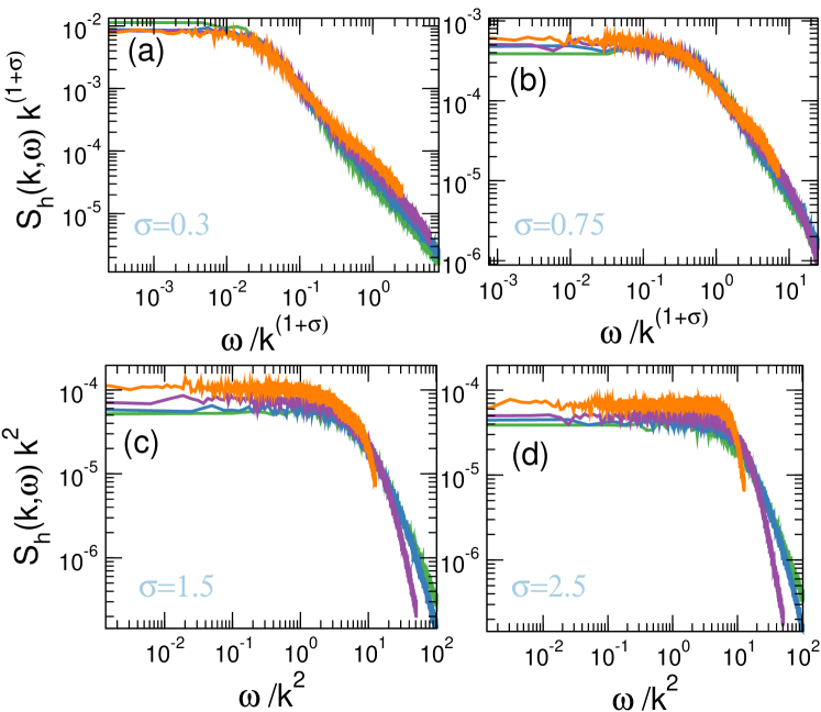
Figure 2: Energy structure factors for the single-well potential case for various values of the range exponent $\sigma$ and different wavenumbers $k=2\pi l/N$, $l=4,8,16,32$s. Simulations with $T=0.2$, $N=2048$ and $\mu=1$.

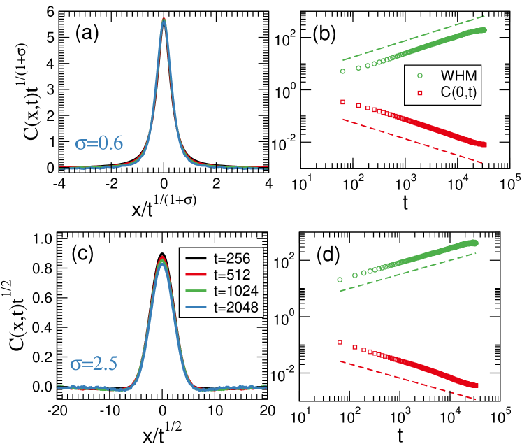
Figure 3: Excess energy correlations $C(x,t)$ for the single-well potential, $\mu=1$, $N=2048$, $T=0.2$ (a,b) $\sigma=0.6$, (c,d) $\sigma=2.5$; Left panels: rescaled correlation, Right panels: the time dependence of the width at half maximum (WHM) and the maxima $C(0,t)$; the dashed lines indicate the power-law scalings $t^{\pm 1/(1+\sigma)}$ (c) and $t^{\pm\frac{1}{2}}$ (d) corresponding to Lévy and normal diffusion respectively. Energy fluctuation are coarse-grained over 4 adjacent lattice sites.

According to the above results, for $\sigma>1$ energy fluctuations obey standard diffusive scaling, as it is well-known for the short-range case. This result matches well with the general expectation that in this regime the long-range terms do not affect the large-scale dynamics and that transport is normal. Conversely, the weak-long range case $0<\sigma<1$ shows an anomalous scaling with a $\sigma$-dependent dynamical exponent.

We can rationalize the results for $0<\sigma<1$ by assuming that fluctuations of the energy field $h(x,t)$ obey the stochastic hydrodynamics equations

$$\dot{h}=-\partial_{x}J$$

$${J}=-\partial_{x}^{\sigma}\left(D_{\sigma}h+\eta\right)$$ (13)

where $\eta(x,t)$ is a standard space-time noise with correlations $\langle\eta(x,t)\eta(x^{\prime},t^{\prime})\rangle=R\delta(t-t^{\prime})\delta(x-x^{\prime})$, $\partial_{x}^{\sigma}$ is a shorthand notation for the fractional derivative of order $\sigma$ (we assume the standard Riesz definition in terms of the Fourier transform) and $D_{\sigma}$ represents a generalized diffusion coefficient. The first equation in (13) is the continuity equation defining the energy current $J$, while the second can be considered as a generalization of the Fourier law to include long-range transport, namely the fact that energy flow is inherently non-local due to nature of the the coupling.

Since (13) is linear we can straightforwardly compute the structure factor by Fourier transform, yielding:

$$S_{h}(k,\omega)\;=\;R\frac{D_{\sigma}|k|^{1+\sigma}}{\omega^{2}+(D_{\sigma}|k|^{1+\sigma})^{2}}$$ (14)

which clearly satisfies (11).

Altogether, we conclude that stochastic fractional diffusion equation (13) is an accurate description of the microscopic model. In Section 4 we will provide an effective stochastic model that accounts for the observations.

3.2 Double-well potential

We now turn to the case of the double-well potential with $\mu>0$. The scaled energy structure factors $S_{h}$ and excess energy correlations $C(x,t)$ for $\sigma=0.6$ are reported in the leftmost panels of figures 4 and 5, respectively for three different energies belonging to the supercritical, critical and subcritical phases. Figures 6 are for $\sigma>1$ where there is no transition. The data are reported under the same rescalings as in the single-well case. They confirm that the dynamical scaling of is the same: relation (11) holds with $z_{h}$ as given in (12), for all the considered energies. Remarkably, this remains true even close to the critical point (see fig. 4c and 5c).

If a critical point exists, one should consider also the dynamics of the magnetization [30] and test whether a dynamical scaling akin to (11) holds for $k,\omega\to 0$, i.e.

$$S_{m}(k,\omega)\;=\;\frac{1}{k^{z_{m}}}\Psi\left(\frac{\omega}{k^{z_{m}}}\right).$$ (15)

As above, $z_{m}=2$ for normal diffusion.

For the magnetization correlator the scaling depends on the energy, see the rightmost panels of figure 4. In the supercritical region, the spectral width of $S_{m}$ is roughly independent of the wavenumber (notice that in the corresponding panel of figure 4b frequencies are not scaled). In the subcritical region $S_{m}$ has instead a large low-frequency component that indeed satisfies relation (15) with the same exponent as $S_{h}$, i.e. $z_{m}=z_{h}=1+\sigma$ for $\sigma<1$. In the critical region the low-frequency component is still present but the quality of data collapse is worse.

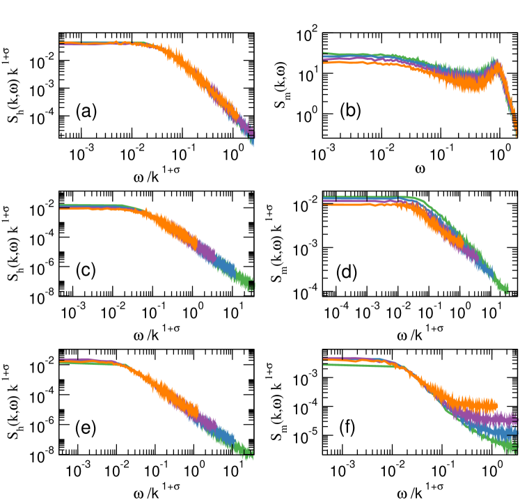
Figure 4: Energy (left) and magnetization (right) structure factors for the double-well potential case for $\mu=1$ $\sigma=0.6$, $N=2048$, $k=2\pi l/N$, $l=4,8,16,32$. Parameters in panels (a,b), (c,d) and (e,f) are for supercritical (paramagnetic) $T=2,e=1.13$, close to critical $T=0.85,e=0.249$, and subcritical $T=0.5,e=-0.42$ (ferromagnetic) regions, respectively.

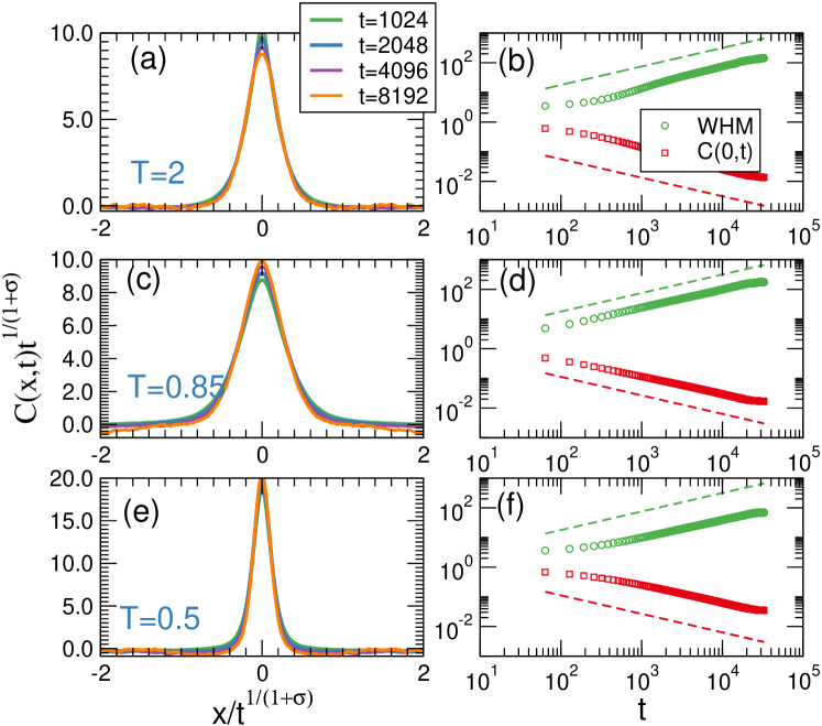
Figure 5: Excess energy correlations $C(x,t)$ for the double-well potential $\mu=1$, $\sigma=0.6$, $N=2048$; Left panels: rescaled correlation; Right panels: time dependence of the width at half maximum (WHM) and of the maxima $C(0,t)$. (a,b) $T=2$, $e=1.13>e_{c}$, (c,d) $T=0.85$, $e=0.249\approx e_{c}$,(e,f) $T=0.5$, $e=-0.42<e_{c}$, the dotted lines indicate the two scalings $t^{\pm 1/(1+\sigma)}$ that correspond to Lévy diffusion. Energy fluctuation are coarse-grained over 4 adjacent lattice sites.

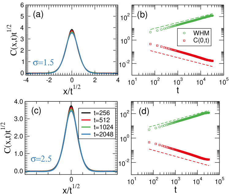
Figure 6: Excess energy correlations $C(x,t)$ for the double-well potential $\mu=1$, $N=2048$, $T=2$; Left panels: rescaled correlation; Right panels: time dependence of the width at half maximum (WHM) and of the maxima $C(0,t)$. (a,b) $\sigma=1.5$, (c,d) $\sigma=2.5$ the dotted lines indicate the two scalings $t^{\pm 1/2}$ that correspond to normal diffusion. Energy fluctuation are coarse-grained over 4 adjacent lattice sites.

Finally, we show in figure 7 the data for the case of repulsive interactions, $\mu<0$. The results are the same as in the attractive case. We thus conclude that hydrodynamics should be the same even in this case.

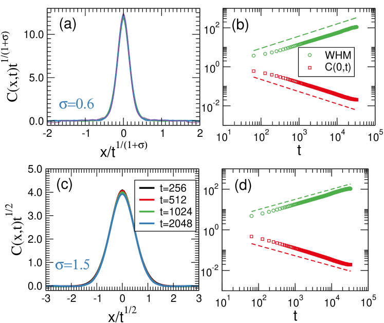
Figure 7: Excess energy correlations $C(x,t)$ for the double-well potential with antiferromagnetic repulsive interaction $\mu=-1$, $N=2048$, $T=2$ (a,b) $\sigma=0.6$, (c,d) $\sigma=1.5$; Left panels: rescaled correlation, Right panels: time dependence of the width at half maximum (WHM) and the maxima $C(0,t)$; the dashed lines indicate the power-law scalings $t^{\pm 1/(1+\sigma)}$ (c) and $t^{\pm\frac{1}{2}}$ (d) corresponding to Lévy and normal diffusion respectively. Energy fluctuation are coarse-grained over 4 adjacent lattice sites.

4 Effective Lévy flight model

The Lévy flight process is well known as the simplest generalization of the Brownian random walk yielding anomalous diffusion of an individual particle [55, 56]. This idea has been recently proposed to describe hydrodynamic fluctuations of a quantum spin chain in the infinite-temperature limit [57]. Let us consider a model where the site energies $h_{j}$ undergo a process in which they are redistributed according to a Lévy flight process, namely a random walk with step sizes drawn from a distribution with algebraic tails. The associated master equation reads

$$\dot{h}_{j}=\sum_{i\neq j}W_{ij}(h_{i}-h_{j}),$$ (16)

with transition rates

$$W_{ij}=\frac{\lambda}{|i-j|^{\nu}}.$$ (17)

where $\lambda$ is a characteristic rate, setting the inverse timescale of the process and $\nu$ is a positive exponent.

In absence of external sources, the dynamical correlation of the model can be computed by Fourier transforming the master equation (16) and considering the large-wavelength limit $k\to 0$ of the field $h(k,t)$. The long-time asymptotics is ruled by long-wavelengths fluctuations. For $1<\nu<3$, taking into account the leading terms in $k$ one obtains (see e.g. [57])

$$\dot{h}(k,t)\approx-\lambda c_{\nu}\,|k|^{\nu-1}h(k,t)$$ (18)

where $c_{\nu}>0$ is a suitable positive constant. Assuming a localized initial state e.g. $h_{j}(t=0)\propto\delta_{j,0}$, then $h(k,0)$ is a constant. Equation (18) can be solved straightforwardly by Laplace transform, yielding

$$|h(k,\omega)|^{2}\propto\frac{\lambda c_{\nu}|k|^{\nu-1}}{\omega^{2}+(\lambda c_{\nu}|k|^{\nu-1})^{2}}$$ (19)

This expression coincides with the structure factor given by (14) upon letting

$$\nu=\sigma+2$$ (20)

and $D_{\sigma}=\lambda c_{\nu}$.

To further validate the stochastic model, we now consider the out-of-equilibrium setup where an ensemble of Lévy fliers is in contact with two reservoirs [7, 8]. To model this situation, we refer to a finite lattice of $N$ sites, assuming periodic boundary conditions. We add to the right hand side of (16) the source terms

$$s_{j}=-\gamma\left[\delta_{j,1}(h_{j}-\varepsilon)+\delta_{j,N/2}(h_{j}+\varepsilon)\right],$$

which tend to force the values of $h_{j}$ to $\pm\varepsilon$ at sites $1,N/2$ respectively, with a rate constant $\gamma$. The resulting master equation is a linear problem that can be solved numerically in the steady state, $\dot{h}_{j}=0$. We compute in particular, $\gamma(h_{1}-\varepsilon)=Q$ and $\gamma(h_{N/2}+\varepsilon)=-Q$ which are the fluxes exchanged with the sources, and the local energy profiles $h_{j}$ in the steady state.

The results are given in fig.8. To ease the comparison with the case of the $\varphi^{4}$ chain, we set $\nu=\sigma+2$ and report the results for a few values of $\sigma$, upon changing $N$. For large $N$ the flux scales as

$$Q\;\propto\;N^{-\sigma}\qquad\rm{for}\quad 0<\sigma<1,$$ (21)

corresponding to superdiffusive transport, while normal transport $Q\propto N^{-1}$ occurs for $\sigma>1$. The case of a dynamical heat channel with Lévy flight is discussed in [58] but the prediction above is not given explicitly there.

It has been argued that standard linear response to a weak external force $F$ breaks down for Lévy flight dynamics [59]. Indeed, the particle mobility is proportional to $F^{\nu-2}$ in the anomalous regime. Equation (21) can be interpreted in the same way, considering the applied thermal gradient $2\varepsilon/N$ as the (thermodynamic) force. Here, this result emerges in a many-body system due to the long-range interactions. A similar conclusion has been drawn in [57] where the spin current of a spin chain has been shown to have the same scaling with respect to an external field. Finally, the scaling (21) is also consistent with the fractional extension of the heat equation as discussed e.g. in [60].

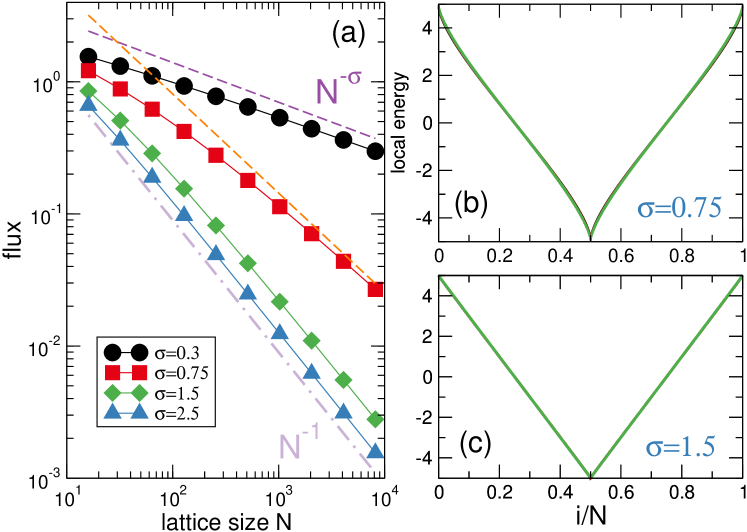
Figure 8: Numerical solution of the Lévy flight master equation in non-equilibrium setup. Equation (16) has been solved in the steady state with a source and a sink located at sites $j=1,N/2$ respectively and $\gamma=1,\epsilon=5$. (a) Scaling of the steady state flux for different exponents showing the anomalous and normal behavior for $\sigma<1$ and $\sigma>1$, respectively. (b,c) Local energy profiles $h_{i}$ versus $i/N$ for two values of $\sigma$. Data for three lattice sizes $N=4096,8192,16384$ are plotted to demonstrate that large-size limit is attained.

5 Nonequilibrium simulations

It is now useful to directly inspect the nonequilibrium behaviour of the long-range $\varphi^{4}$ model (1). We consider an analogous transport setup where a $\varphi^{4}$ chain with periodic boundary conditions interacts with two Maxwellian heat baths placed at antipodal positions. Such reservoirs introduce elastic collisions with a model of ideal gas in equilibrium and impose two different temperatures $T_{A}\neq T_{B}$ in regions $A$ and $B$ of the chain. Collisions occur at random times drawn independently from a Poissonian distribution $P(t)=\gamma_{M}\exp(-\gamma_{M}t)$, where $\gamma_{M}$ defines the strength of the coupling [1, 24]. In between two consecutive collision events, the chain is evolved microcanonically with a symplectic fourth-order integration algorithm [51]. In order to reduce boundary effects, we let each reservoir interact with an extensive number $n_{r}=N/16$ of $\varphi^{4}$ lattice sites. Accordingly, at each collision time, $n_{r}$ independent collisions are generated on each thermalized region. Heat fluxes are measured as the time average of the total kinetic energy transferred from the reservoir to the particles belonging to the same thermalized region. More precisely, for region $A$ we define the flux

$$Q_{A}=\overline{\sum_{i\in A}\delta K_{i}(t)}\,,$$ (22)

where $\delta K_{i}(t)$ is the local variation of kinetic energy on site $i$ after a collision event and the bar denotes a time average. An analogous expression holds for $Q_{B}$ and a nonequilibrium steady state is reached when $Q_{A}=-Q_{B}\equiv Q$.

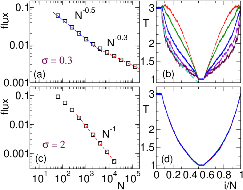
Figure 9: (a) Scaling of the stationary exchanged heat flux $Q$ versus lattice size for a $\varphi^{4}$ chain with $\sigma=0.3$ in contact with two reservoirs with $T_{A}=3$ and $T_{B}=1$. (b) The corresponding temperature profiles versus $i/N$: curves from top to bottom correspond to $N=1024$, 4096, 16384, 65536, 131072. The cyan dashed line is a one-parameter fit of the function $T(\tilde{y})=T_{A}(1-\tilde{y}^{\delta})$ (see text) with $\delta\simeq 0.43$ and fixed $T_{A}=3$. (c) Exchanged heat flux for $\sigma=2$ and same thermal boundary conditions. (d) Temperature profiles for $\sigma=2$ and $N=1024$, 4096, 16384. Nonequilibrium observables are averaged over a time up to $2\cdot 10^{7}$ units after a transient of at least $10^{6}$ units.

In the following, we restrict ourselves to the case of the single-well local potential with parameter $\mu=2$ and we choose $\gamma_{M}=1$. We have verified that this choice of parameters allows to optimize heat fluxes for temperatures $T_{A}=3$ and $T_{B}=1$ considered in our simulations. In Fig. 9(a) we show the scaling of the stationary flux versus the lattice size $N$ for $\sigma=0.3$. Data appear to be initially well represented a power law $Q\simeq N^{-0.5}$ for a rather broad range of sizes, while they subsequently bend to the scaling $Q\simeq N^{-\sigma}$, in agreement with the Lévy flight model. The crossover between the two scaling laws is found to occur for $N\simeq 5000$. This evidence confirms that finite-size effects have an important role in the study of transport properties of long-range systems, as discussed in [24].

Further information is obtained from the shape of the stationary profiles of temperature measured along the chain and reported as functions of the rescaled spatial variable $y=i/N$, see Fig. 9(b). To the best of our numerical accuracy, we have some evidence that the profiles tend to approach a highly nonlinear curve in the limit of large $N$, although some deviations are still present for the largest sizes here investigated. The temperature drop in the first half of the chain for the largest size $N=131072$ (see the continuous bottom line) is well fitted by the function $T(\tilde{y})=T_{A}(1-\tilde{y}^{\delta})$, where $\tilde{y}=(y-n_{r}/N)$ is the shifted spatial variable restricted to $n_{r}/N\leq y\leq 1/2$, see dashed line. The fitted value of the exponent $\delta\simeq 0.43$ signals the presence of a singularity of the derivative of $T(\tilde{y})$ in $\tilde{y}=0$, i.e. at the boundary with the thermalized region. On the other hand, finite-size effects deeply modify the shape of the profiles for smaller sizes, see the upper solid line corresponding to $N=1024$, which exhibits a nearly vanishing first derivative close to $\tilde{y}=0$ and a negative second derivative.

Finally, in the region $\sigma>1$ numerical simulations confirm the occurrence of normal transport $Q\simeq N^{-1}$, as shown in Fig. 9(c) for $\sigma=2$. The corresponding temperature profiles displayed in Fig. 9(d) are smooth and characterized by a very clean overlap, with a manifest reduction of finite-size effects with respect to the long-range regime. Unlike the Lévy flight model (see Fig. 8(c)), they also manifest a clear deviation from the linear profile. We argue that this is due to a slight dependence of the $\varphi^{4}$ diffusion constant on temperature in analogy with what observed in similar oscillators models [61].

6 Discussion

We have demonstrated that the fractional diffusion process and the Lévy flight model well account for the large-scale energy fluctuations of the long-range $\varphi^{4}$ chain. In hindsight, this may seem trivial in view of the very fact that the couplings decay algebraically with the distance. However this is not the case for at least two reasons. First of all, the correct exponent is given by (20), a relation which was not foreseen a priori. Second, models with the same $r^{-1-\sigma}$ interactions like the Hamiltonian XY model [21] or the Fermi-Pasta-Ulam-Tsingou model [62] have different dynamical exponents. In other words, models having the same coupling $r^{-1-\sigma}$ may belong to different dynamical universality classes, having different hydrodynamics.

This conclusion is confirmed also by noting the differences between our model and the momentum-exchange model with long-range interactions, recently studied in [63]. The Authors considered the Hamiltonian (6) with a quadratic pinning potential perturbed by a random exchange of momenta between the nearest neighbor sites, occurring with a give rate. The dependence of the exponent ruling the decay of energy current autocorrelation (and thus the finite-size scaling of the heat flux in the nonequilibrum setup) has a dependence on $\sigma$ which is different from ours. In their model superdiffusive transport occurs for $\frac{1}{2}<\sigma<\frac{3}{2}$ while here it happens for $0<\sigma<1$. Also, even if their model leads to a fractional diffusion in the hydrodynamic limit [64] which is the same as (13), the dependence of the order of the fractional derivative is different. We thus argue that the two models belong to different classes.

As far as scaling is concerned, anomalous energy diffusion appears not to be affected by the fact that the $\varphi^{4}$ with a double-well potential undergoes the phase transition. As shown in fig. 4, even very close to the critical point the hydrodynamic behavior of the energy field still follows the fractional diffusion equation. From our study we cannot exclude a sensitive dependence of thermal coefficients like e.g. $D_{\sigma}$ on energy around criticality, as seen for instance in the Ising model [31, 32]. Nonetheless, this observation is noteworthy and requires a theoretical explanation. It has already been argued in [39] that for Hamiltonian dynamics there is a coupling between the local temperature field and order parameter fields. So one might wonder how to include this effect in the hydrodynamics. The standard approach [30] amounts to add to the dynamics of $m$ the one of the energy $h$, which is conserved and thus slow regardless of the closeness to the critical point. This leads to Model C (see e.g. eqs. (4.50) in [30]) that includes a conserved diffusive field. Its physical interpretation is that slow energy/temperature fluctuations modulate the coefficient $a_{2}$ in the Ginzburg-Landau functional. It could be argued that the same would occur in the long-range case and this would require adding to eq. (13) an equation for $m$ that accounts for the hydrodynamic behavior of the magnetization in the low-temperature phase. This should be subject of future studies.

Finally, in the present work we focused on equilibrium correlations and on steady-state transport. One may thus wonder which is the connection with transient non-equilibrium problems. An important example in this context is the phenomenon of coarsening dynamics, which has been studied in detail for the one-dimensional Ising model with long-range interactions (see [65] and references therein for a recent account) and for the present model [39]. Actually the dynamical exponent measured by equilibrium correlations is not related to the one characteristic of coarsening dynamics as measured in [39]. The latter is essentially determined by kinetics of domain walls [65].

7 Summary and conclusions

We have reported a simulation study of the discretized $\varphi^{4}$ lattice theory in one dimension, with long-range interactions decaying as an inverse power $r^{-1-\sigma}$ of the intersite distance $r$, and $\sigma>0$. We presented a dynamical scaling analysis of the relevant observable, energy structure factors and excess energy correlations. Large-scale fluctuations of the local energy field display hydrodynamic behavior, which is diffusive for $\sigma>1$ and superdiffusive for $0<\sigma<1$ in both the cases with single and double-well local potentials, with either attractive and repulsive couplings. In the superdiffusive case, numerical data suggest that hydrodynamic correlations are described by a fractional diffusion equation of order $\sigma$, eq. (13). In the case of the double-well potential with attractive interaction such behavior of energy fluctuations appear to be insensitive to the phase transition. To further support the interpretation of the correlation data, we have successfully compared both equilibrium and nonequilibrium simulations with an effective model of transport based on Lévy flights of energy carriers. Altogether we conclude that the $\varphi^{4}$ model belongs to a different dynamical universality class with respect to others systems studied in the literature so far. We expect that the same conclusions apply to the class of Hamiltonians (1) with different local potentials $U(q)$. Our data will be of help to understand the large-scale properties of long-range interacting classical and quantum many-body systems.

References

References

- [1] Lepri S, Livi R and Politi A 2003 Phys. Rep. 377 1
- [2] Dhar A 2008 Adv. Phys. 57 457–537
- [3] Lepri S (ed) 2016 Thermal transport in low dimensions: from statistical physics to nanoscale heat transfer (Lect. Notes Phys vol 921) (Springer-Verlag, Berlin Heidelberg)
- [4] Benenti G, Lepri S and Livi R 2020 Frontiers in Physics 8 292 URL https://www.frontiersin.org/article/10.3389/fphy.2020.00292
- [5] Zaburdaev V, Denisov S and Klafter J 2015 Reviews of Modern Physics 87 483
- [6] Cipriani P, Denisov S and Politi A 2005 Phys. Rev. Lett. 94 244301
- [7] Lepri S and Politi A 2011 Phys. Rev. E 83 030107
- [8] Dhar A, Saito K and Derrida B 2013 Phys. Rev. E 87 010103
- [9] Lepri S, Mejía-Monasterio C and Politi A 2010 Journal of Physics A: Mathematical and Theoretical 43 065002 URL https://doi.org/10.1088/1751-8113/43/6/065002
- [10] Basile G, Bernardin C, Jara M, Komorowski T and Olla S 2016 Thermal conductivity in harmonic lattices with random collisions Thermal transport in low dimensions (Springer) pp 215–237
- [11] Cividini J, Kundu A, Miron A and Mukamel D 2017 J. Stat. Mech: Theory Exp. 2017 013203
- [12] Dhar A, Kundu A and Kundu A 2019 Frontiers in Physics 7 159
- [13] Spohn H 2014 J. Stat. Phys. 154 1191–1227
- [14] Mendl C B and Spohn H 2013 Phys. Rev. Lett. 111(23) 230601
- [15] Das S, Dhar A and Narayan O 2014 J. Stat. Phys.; 154 204–213 ISSN 0022-4715
- [16] Mendl C B and Spohn H 2015 Journal of Statistical Mechanics: Theory and Experiment 2015 P03007
- [17] Lepri S, Livi R and Politi A 2020 Physical Review Letters 125 040604
- [18] Torcini A and Lepri S 1997 Phys. Rev. E 55 R3805
- [19] Métivier D, Bachelard R and Kastner M 2014 Phys. Rev. Lett. 112 210601
- [20] Ávila R R, Pereira E and Teixeira D L 2015 Physica A: Statistical Mechanics and its Applications 423 51–60
- [21] Olivares C and Anteneodo C 2016 Phys. Rev. E 94(4) 042117
- [22] Bagchi D 2017 Phys. Rev. E 95 032102
- [23] Bagchi D 2017 Phys. Rev. E 96 042121
- [24] Iubini S, Di Cintio P, Lepri S, Livi R and Casetti L 2018 Phys. Rev. E 97(3) 032102
- [25] Wang J, Dmitriev S V and Xiong D 2020 Physical Review Research 2 013179
- [26] Bouchet F, Gupta S and Mukamel D 2010 Physica A: Statistical Mechanics and its Applications 389 4389–4405
- [27] Campa A, Dauxois T and Ruffo S 2009 Phys. Rep. 480 57–159
- [28] Campa A, Dauxois T, Fanelli D and Ruffo S 2014 Physics of long-range interacting systems (OUP Oxford)
- [29] de Buyl P, De Ninno G, Fanelli D, Nardini C, Patelli A, Piazza F and Yamaguchi Y Y 2013 Physical Review E 87 042110
- [30] Hohenberg P C and Halperin B I 1977 Reviews of Modern Physics 49 435
- [31] Harris R and Grant M 1988 Physical Review B 38 9323
- [32] Saito K, Takesue S and Miyashita S 1999 Physical Review E 59 2783
- [33] Colangeli M, Giardina C, Giberti C and Vernia C 2018 Physical Review E 97 030103
- [34] Bermúdez A, Bruderer M and Plenio M B 2013 Physical review letters 111 040601
- [35] Ramm M, Pruttivarasin T and Häffner H 2014 New Journal of Physics 16 063062
- [36] Richerme P, Gong Z X, Lee A, Senko C, Smith J, Foss-Feig M, Michalakis S, Gorshkov A V and Monroe C 2014 Nature 511 198–201
- [37] Molerón M, Chong C, Martínez A J, Porter M A, Kevrekidis P G and Daraio C 2019 New Journal of Physics 21 063032
- [38] Defenu N, Donner T, Macrì T, Pagano G, Ruffo S and Trombettoni A 2021 arXiv preprint arXiv:2109.01063
- [39] Staniscia F, Bachelard R, Dauxois T and De Ninno G 2019 EPL (Europhysics Letters) 126 17001
- [40] Hu B, Li B and Zhao H 2000 Physical Review E 61 3828
- [41] Aoki K and Kusnezov D 2000 Phys. Lett. A 265 250
- [42] Piazza F and Lepri S 2009 Phys. Rev. B 79(9) 094306 URL https://link.aps.org/doi/10.1103/PhysRevB.79.094306
- [43] Krumhansl J and Schrieffer J 1975 Physical Review B 11 3535
- [44] Dyson F J 1969 Communications in Mathematical Physics 12 91–107
- [45] Mukamel D 2009 arXiv preprint arXiv:0905.1457
- [46] Desai R C and Zwanzig R 1978 Journal of Statistical Physics 19 1–24
- [47] Dauxois T, Lepri S and Ruffo S 2003 Communications in Nonlinear Science and Numerical Simulation 8 375–387
- [48] Aizenman M, Chayes J, Chayes L and Newman C 1988 Journal of Statistical Physics 50 1–40
- [49] Kerimov A 1993 Journal of statistical physics 72 571–620
- [50] Gupta S, Campa A and Ruffo S 2014 Journal of Statistical Mechanics: Theory and Experiment 2014 R08001
- [51] McLachlan R I and Atela P 1992 Nonlinearity 5 541
- [52] Caiani L, Casetti L and Pettini M 1998 Journal of Physics A: Mathematical and General 31 3357
- [53] Zhao H 2006 Phys. Rev. Lett. 96 140602
- [54] Li Y, Liu S, Li N, Hänggi P and Li B 2015 New J. Phys. 17 043064
- [55] Metzler R and Klafter J 2000 Physics reports 339 1–77
- [56] Klages R, Radons G and Sokolov I M (eds) 2008 Anomalous Transport: Foundations and Applications (Wiley-VCH Verlag, Weinheim)
- [57] Schuckert A, Lovas I and Knap M 2020 Phys. Rev. B 101(2) 020416 URL https://link.aps.org/doi/10.1103/PhysRevB.101.020416
- [58] Denisov S, Klafter J and Urbakh M 2003 Phys. Rev. Lett. 91 194301
- [59] Arkhincheev V 2001 Nonlinear relation between diffusion and conductivity for Lévy flights AIP Conference Proceedings vol 553 (American Institute of Physics) pp 231–235
- [60] Li S N and Cao B Y 2020 Applied Mathematics Letters 99 105992
- [61] Iubini S, Lepri S, Livi R and Politi A 2016 New J. Phys. 18 083023
- [62] Di Cintio P, Iubini S, Lepri S and Livi R 2019 Journal of Physics A: Mathematical and Theoretical 52 274001
- [63] Tamaki S and Saito K 2020 Physical Review E 101 042118
- [64] Suda H 2019 arXiv preprint arXiv:1912.01753
- [65] Corberi F, Lippiello E and Politi P 2019 Journal of Statistical Mechanics: Theory and Experiment 2019 074002