Polarized Gluon Pseudodistributions at Short Distances

Abstract

We formulate the basic points of the pseudo-PDF approach to the lattice calculation of polarized gluon PDFs. We present the results of our calculations of the one-loop corrections for the bilocal $G_{\mu\alpha}(z)\widetilde{G}_{\lambda\beta}(0)$ correlator of gluonic fields. Expressions are given for a general situation when all four indices are arbitrary, and also for specific combinations of indices corresponding to three matrix elements that contain the twist-2 invariant amplitude related to the polarized PDF. We study the evolution properties of these matrix elements, and derive matching relations between Euclidean and light-cone Ioffe-time distributions. These relations are necessary for extraction of the polarized gluon distributions from the lattice data.

1 Introduction

Lattice calculations devoted to extraction of the parton distribution functions (PDFs) have attracted recently a considerable interest (see Refs. Constantinou:2020hdm ; Cichy:2018mum for reviews and references). Starting with the paper Ji:2013dva by X. Ji, modern efforts aim at directly getting PDFs $f(x)$ as functions of the momentum fraction variable $x$ rather than just calculating their $x^{N}$ moments. The key element of these efforts is the analysis of equal-time bilocal operators that define various parton functions, in particular, PDFs, distribution amplitudes (DAs), generalized parton distributions (GPDs), and transverse momentum dependent distributions (TMDs). The major object of Ji’s approach in the case of ordinary PDFs, are quasi-PDFs $Q(y,p_{3})$ Ji:2013dva ; Ji:2014gla . To get the PDFs from them, one should take the large-momentum $p_{3}\to\infty$ limit of $Q(y,p_{3})$.

There are alternative methods based on the coordinate-space formulation, such as the “good lattice cross sections” approach Ma:2014jla ; Ma:2017pxb and the pseudo-PDF approach Radyushkin:2017cyf ; Radyushkin:2017sfi ; Orginos:2017kos , in which the equal-time correlators $M(z_{3},p_{3})$ are considered as functions of the Ioffe-time Braun:2007wv ; Bali:2017gfr ; Bali:2018spj $\nu=z_{3}p_{3}$ and the probing scale parameter $z_{3}^{2}$. In these latter cases, the parton distributions are extracted by taking the short-distance $z_{3}^{2}\to 0$ limit at fixed $\nu$.

To convert the data measured on a Euclidean lattice into the PDFs defined on the light cone, it should be taken into account that the limits $p_{3}\to\infty$ and $z_{3}\to 0$ are singular. To perform the conversion in such a situation, one needs to derive and use matching relations.

In the quasi-PDF approach, the matching relations were derived for quark Ji:2013dva ; Xiong:2013bka ; Ji:2015jwa ; Izubuchi:2018srq and gluon PDFs Wang:2017eel ; Wang:2017qyg ; Wang:2019tgg , and also for GPDs Ji:2015qla ; Xiong:2015nua ; Liu:2019urm and the pion DA Ji:2015qla .

The matching relations for the bilocal operators in the coordinate representation were originally derived in applications to quark nonsinglet PDFs Ji:2017rah ; Radyushkin:2017lvu ; Radyushkin:2018cvn ; Zhang:2018ggy ; Izubuchi:2018srq . The pseudo-PDF procedure for lattice extraction of nonforward parton functions, such as nonsinglet GPDs and the pion DA were described in Ref. Radyushkin:2019owq , where the necessary matching conditions were also obtained.

The pseudo-PDF approach to the extraction of unpolarized gluon PDFs was formulated in our paper Balitsky:2019krf (see also Ref. Balitsky:2021bds ). The results of one-loop calculations for the gluon bilocal operators were presented there, and, in a more detailed form in Ref. Balitsky:2021qsr . The matching conditions following from these results have been used in lattice extractions of the unpolarized gluon PDFs in Refs. Fan:2020cpa ; Fan:2021bcr and HadStruc:2021wmh . One-loop corrections to the matrix element of the twist-4 “gluon condensate” operator $G^{\mu\nu}(0)G_{\mu\nu}(z)$ have been recently obtained in the momentum-representation calculation of Ref. Radyushkin:2021fel .

In the present work, we describe the basics of the pseudo-PDF approach to lattice extraction of the polarized gluon PDFs. The paper is organized as follows. In Section 2, we investigate kinematic structure of the polarized matrix elements of the gluonic bilocal operators built from the gluon stress-tensor and its dual. In particular, we identify the matrix elements that contain information about the twist-2 polarized gluon PDF. In Section 3, we present the results for one-loop corrections to the bilocal operator, and discuss their ultraviolet and short-distance behavior. The matching relations necessary for the lattice extraction of the polarized gluon PDFs are derived in Section 4. The summary of the paper is given in section 5.

2 Matrix elements

2.1 Definitions

To extract polarized gluon distributions of a nucleon, we consider matrix elements of bilocal operators $G_{\mu\alpha}(z)\widetilde{G}_{\lambda\beta}(0)$ composed of two gluon fields, with the dual field defined by $\widetilde{G}_{\lambda\beta}=\frac{1}{2}\epsilon_{\lambda\beta\rho\gamma}G^{\rho\gamma}$. The matrix elements are specified by

$$\widetilde{m}_{\mu\alpha;\lambda\beta}(z,p)\equiv\langle p,s|\,G_{\mu\alpha}(z)\,{\tilde{E}}(z,0;A)\widetilde{G}_{\lambda\beta}(0)|p,s\rangle\ ,$$ (1)

where ${\tilde{E}}(z,0;A)$ is the usual $0\to z$ straight-line gauge link in the gluon (adjoint) representation

$${\tilde{E}}(z,0;A)\equiv P\exp\left[ig\,z_{\sigma}\,\int_{0}^{1}dt\,\tilde{A}^{\sigma}(tz)\right]\ .$$ (2)

The standard definition of the polarized gluon PDFs Manohar:1990jx uses the contracted amplitude $g^{\alpha\lambda}{m}_{\mu\alpha;\lambda\beta}$, but we will keep all four indices $\mu,\alpha,\lambda,\beta$ non-contracted. The part that depends on the nucleon spin is determined by the $z$-odd combination, which vanishes for the unpolarized case and is linear in the spin-vector $s$. Thus, we start with the amplitude

$$\widetilde{M}_{\mu\alpha;\lambda\beta}(z,p)\equiv\widetilde{m}_{\mu\alpha;\lambda\beta}(z,p)-\widetilde{m}_{\mu\alpha;\lambda\beta}(-z,p)\ .$$ (3)

To simplify further formulas, we normalize $s_{\mu}$ by $s^{2}=-m^{2}$, where $m$ is the nucleon mass. This means that our polarization vector $s_{\mu}$ is related by $s_{\mu}=mS_{\mu}$ to the usual polarization vector $S_{\mu}$ which is normalized by $S^{2}=-1$.

2.2 Invariant amplitudes

The tensor structures for the decomposition of $\widetilde{M}_{\mu\alpha;\lambda\beta}(z,p)$ over invariant amplitudes may be built from two available 4-vectors $p_{\alpha}$, $z_{\alpha}$, one pseudo-vector $s_{\alpha}$ and the metric tensor $g_{\alpha\beta}$. These structures must be anti-symmetric with respect to interchange of both $\{\mu\leftrightarrow\alpha\}$ and $\{\lambda\leftrightarrow\beta\}$.

Let us list first the structures in which $s$ carries one of the ${\mu\alpha;\lambda\beta}$ indices. Such structures, before the anti-symmetrization, may have two possible forms: $s_{\alpha}A_{\beta}g_{\mu\lambda}$ and $s_{\alpha}A_{\beta}B_{\mu}C_{\lambda}$, where $A,B,C$ correspond to $p$ or $z$. Incorporating the antisymmetry of $G_{\rho\sigma}$ with respect to its indices, we have

$$\widetilde{M}_{\mu\alpha;\lambda\beta}^{(1)}(z,p)= \left(g_{\mu\lambda}s_{\alpha}p_{\beta}-g_{\mu\beta}s_{\alpha}p_{\lambda}-g_{\alpha\lambda}s_{\mu}p_{\beta}+g_{\alpha\beta}s_{\mu}p_{\lambda}\right)\widetilde{\mathcal{M}}_{sp}$$

$$+ \left(g_{\mu\lambda}p_{\alpha}s_{\beta}-g_{\mu\beta}p_{\alpha}s_{\lambda}-g_{\alpha\lambda}p_{\mu}s_{\beta}+g_{\alpha\beta}p_{\mu}s_{\lambda}\right)\widetilde{\mathcal{M}}_{ps}$$

$$+ \left(g_{\mu\lambda}s_{\alpha}z_{\beta}-g_{\mu\beta}s_{\alpha}z_{\lambda}-g_{\alpha\lambda}s_{\mu}z_{\beta}+g_{\alpha\beta}s_{\mu}z_{\lambda}\right)\widetilde{\mathcal{M}}_{sz}$$

$$+ \left(g_{\mu\lambda}z_{\alpha}s_{\beta}-g_{\mu\beta}z_{\alpha}s_{\lambda}-g_{\alpha\lambda}z_{\mu}s_{\beta}+g_{\alpha\beta}z_{\mu}s_{\lambda}\right)\widetilde{\mathcal{M}}_{zs}$$

$$+ (p_{\mu}s_{\alpha}-p_{\alpha}s_{\mu})(p_{\lambda}z_{\beta}-p_{\beta}z_{\lambda})\widetilde{\mathcal{M}}_{pspz}+(p_{\mu}z_{\alpha}-p_{\alpha}z_{\mu})(p_{\lambda}s_{\beta}-p_{\beta}s_{\lambda})\widetilde{\mathcal{M}}_{pzps}$$

$$+ (s_{\mu}z_{\alpha}-s_{\alpha}z_{\mu})(p_{\lambda}z_{\beta}-p_{\beta}z_{\lambda})\widetilde{\mathcal{M}}_{szpz}+(p_{\mu}z_{\alpha}-p_{\alpha}z_{\mu})(s_{\lambda}z_{\beta}-s_{\beta}z_{\lambda})\widetilde{\mathcal{M}}_{pzsz}\ ,$$ (4)

where the invariant amplitudes $\widetilde{\mathcal{M}}$ are functions of the invariant interval $z^{2}$ and the Ioffe time Braun:1994jq $(pz)\equiv-\nu$ (the minus sign here is introduced to have $\nu=p_{3}z_{3}$ when $z=\{0,0,0,z_{3}\}$).

There are also structures containing $s$ through the $(sz)$ product accompanied by all the tensor combinations of $p,z$ and metric tensor that have been used in Ref. Balitsky:2019krf for the unpolarized case. These combinations, before the anti-symmetrization, may have three possible forms: $A_{\alpha}B_{\beta}g_{\mu\lambda}$, $A_{\alpha}B_{\beta}C_{\mu}D_{\lambda}$ and $g_{\alpha\beta}g_{\mu\lambda}$, where $A,B,C,D$ correspond to one of $p$ or $z$. Thus, we have

$$\widetilde{M}_{\mu\alpha;\lambda\beta}^{(2)}(z,p)= (sz)\left(g_{\mu\lambda}p_{\alpha}p_{\beta}-g_{\mu\beta}p_{\alpha}p_{\lambda}-g_{\alpha\lambda}p_{\mu}p_{\beta}+g_{\alpha\beta}p_{\mu}p_{\lambda}\right)\widetilde{\mathcal{M}}_{pp}$$

$$+ (sz)\left(g_{\mu\lambda}z_{\alpha}z_{\beta}-g_{\mu\beta}z_{\alpha}z_{\lambda}-g_{\alpha\lambda}z_{\mu}z_{\beta}+g_{\alpha\beta}z_{\mu}z_{\lambda}\right)\widetilde{\mathcal{M}}_{zz}$$

$$+ (sz)\left(g_{\mu\lambda}z_{\alpha}p_{\beta}-g_{\mu\beta}z_{\alpha}p_{\lambda}-g_{\alpha\lambda}z_{\mu}p_{\beta}+g_{\alpha\beta}z_{\mu}p_{\lambda}\right)\widetilde{\mathcal{M}}_{zp}$$

$$+ (sz)\left(g_{\mu\lambda}p_{\alpha}z_{\beta}-g_{\mu\beta}p_{\alpha}z_{\lambda}-g_{\alpha\lambda}p_{\mu}z_{\beta}+g_{\alpha\beta}p_{\mu}z_{\lambda}\right)\widetilde{\mathcal{M}}_{pz}$$

$$+ (sz)\left(p_{\mu}z_{\alpha}-p_{\alpha}z_{\mu}\right)\left(p_{\lambda}z_{\beta}-p_{\beta}z_{\lambda}\right)\widetilde{\mathcal{M}}_{ppzz}$$

$$+ (sz)\left(g_{\mu\lambda}g_{\alpha\beta}-g_{\mu\beta}g_{\alpha\lambda}\right)\widetilde{\mathcal{M}}_{gg}\ .$$ (5)

One may propose to check if we may also use the Levi-Civita tensor like $\epsilon_{\gamma\delta\rho\sigma}$ for building possible tensor structures. Here we note that our matrix element $\widetilde{M}_{\mu\alpha;\lambda\beta}$ is a pseudo-tensor. Furthermore, it should be linear in the nucleon polarizations vector $s_{\gamma}$, which is a pseudo-vector. Hence, the Levi-Civita pseudo-tensor $\epsilon_{\star\star\star\star}$ should appear twice in a particular tensor structure involving $s_{\gamma}$. However, the product of two Levi-Civita tensors $\epsilon_{\star\star\star\star}\epsilon_{\star\star\star\star}$ may be always written in terms of (sums of products of) metric tensors $g_{\star\star}$ . Thus, the combinations listed in Eqs. (4) and (5) exhaust all the possibilities for tensor structures compliant with the Lorentz covariance and antisymmetry of $G_{\rho\sigma}$ with respect to its indices.

In fact, our operator has the structure $\epsilon_{\lambda\beta\rho\gamma}G^{\lambda\beta}(z)G^{\rho\gamma}(0)$, where $G(z)$ and $G(0)$ is the same field. As we will see in Sect. (2.5), this imposes two relations (28), (33) between some invariant amplitudes $\widetilde{\mathcal{M}}$ parametrizing $\widetilde{M}_{\mu\alpha;\lambda\beta}^{(2)}$ and invariant amplitudes entering into $\widetilde{M}_{\mu\alpha;\lambda\beta}^{(1)}$. One may also incorporate the symmetry properties of $\widetilde{M}_{\mu\alpha;\lambda\beta}(z,p)$ with respect to $z$. Namely, since $\widetilde{M}_{\mu\alpha;\lambda\beta}(z,p)$ is odd in $z$, the invariant amplitudes $\widetilde{\mathcal{M}}_{sp},\widetilde{\mathcal{M}}_{ps},\widetilde{\mathcal{M}}_{pzsz},\widetilde{\mathcal{M}}_{szpz}$, $\widetilde{\mathcal{M}}_{zp},\widetilde{\mathcal{M}}_{pz}$ are odd functions of $\nu$, while the remaining ones are even functions of $\nu$.

Such a decomposition of $\widetilde{M}_{\mu\alpha;\lambda\beta}(z,p)$ is quite general. But it may be also constructed, in particular, from a formal Taylor expansion of $G_{\mu\alpha}(z)\,{\tilde{E}}(z,0;A)\widetilde{G}_{\lambda\beta}(0)$ over local operators, followed by taking their matrix elements and then recombining back the terms with the same tensor structure. The implicit assumption of this procedure is that such a Taylor expansion exists.

In QCD, $\widetilde{M}_{\mu\alpha;\lambda\beta}(z,p)$ has singularities on the light cone $z^{2}=0$ due to perturbative logarithms $\ln(-z^{2})$ generated by gluonic corrections. Thus, we will assume that the invariant amplitudes $\widetilde{\mathcal{M}}(\nu,z^{2})$ are finite for $z^{2}=0$ at the tree level, and will explicitly calculate the perturbative one-loop corrections that produce the $\ln(-z^{2})$ terms.

2.3 Relation to PDF

The usual light-cone polarized gluon distribution $\Delta g(x)$ is obtained Manohar:1990jx from the matrix element $g^{\alpha\beta}\widetilde{M}_{+\alpha;\beta+}(z,p)$, with $z$ taken in the light-cone “minus” direction, $z=z_{-}$. In terms of the parametrization written above, we have

$$g^{\alpha\beta} \widetilde{M}_{+\alpha;\beta+}(z_{-},p)=-2p_{+}s_{+}\left[\widetilde{\mathcal{M}}_{ps}^{(+)}(\nu,0)+p_{+}z_{-}\widetilde{\mathcal{M}}_{pp}(\nu,0)\right]\ ,$$ (6)

where ${\widetilde{\mathcal{M}}}_{ps}^{(+)}\equiv{\widetilde{\mathcal{M}}}_{ps}+\widetilde{\mathcal{M}}_{sp}$. Thus, the PDF is determined by the structure

$${\widetilde{\mathcal{M}}}_{ps}^{(+)}-\nu\widetilde{\mathcal{M}}_{pp}\equiv-i{\cal I}_{p}(\nu)\ .$$ (7)

More specifically,

$${\cal I}_{p}(\nu)=\frac{i}{2}\int_{-1}^{1}dx\,e^{-ix\nu}x\Delta g(x)\,\ .$$ (8)

Thus, to extract $x\Delta g(x)$, we should choose the operators with particular combinations of the $\{\mu\alpha;\lambda\beta\}$ indices that contain $\widetilde{\mathcal{M}}_{ps}^{(+)}$ and $\widetilde{\mathcal{M}}_{pp}$ in their parametrization.

It is worth stressing that it is the momentum-weighted density $x\Delta g(x)$ that is a natural quantity in this definition of the polarized gluon PDF. Since $\widetilde{M}_{+\alpha;\beta+}(z_{-},p)$ is an odd function of $z$, $x\Delta g(x)$ is an odd function of $x$. Hence, ${\cal I}_{p}(\nu)$ is an odd function of $\nu$, and, for $\nu>0$ it can be written as a sine transform

$${\cal I}_{p}(\nu)=\int_{0}^{1}dx\,\sin(x\nu)\,x\Delta g(x)\,\ .$$ (9)

An important quantity is the spin $\Delta G$ contributed by the gluons to the total nucleon spin. It is given by the integral of $\Delta g(x)$ over all positive $x$. As noted in Ref. Braun:1994jq , this integral may also be written as an integral over the Ioffe-time distribution

$$\Delta G\equiv\int_{0}^{1}dx\,\Delta g(x)=\int_{0}^{\infty}d\nu\,{\cal I}_{p}(\nu)\,\ .$$ (10)

Thus, to estimate $\Delta G$, it is sufficient to know the Ioffe-time distribution ${\cal I}_{p}(\nu)$, without converting it into the PDF $\Delta G(x)$.

2.4 Matrix elements for extraction of $\Delta g(x)$

Since the gluon tensor $G_{\rho\sigma}$ is antisymmetric with respect to its indices, the values $\alpha=+$ and $\beta=+$ may be taken off the summation in Eq. (6). Furthermore, since $g_{--}=0$, the combination $g^{\alpha\beta}\widetilde{M}_{+\alpha;\beta+}(z,p)$ involves the summation over the transverse indices $i,j=1,2$ only, i.e. it reduces to $g^{ij}\widetilde{M}_{+i;j+}(z,p)\equiv\widetilde{M}_{+i;+i}(z,p)$ (summation over $i$ implied), for which we have

$$\widetilde{M}_{+i;+i}=\widetilde{M}_{0i;0i}+\widetilde{M}_{3i;3i}+\widetilde{M}_{0i;3i}+\widetilde{M}_{3i;0i}\ .$$ (11)

When $z$ has just the third component, i.e., $z=z_{3}$, the decomposition of these combinations in the basis of the $\widetilde{\mathcal{M}}$ structures is given by

$$\widetilde{M}_{0i;0i}= -2s_{0}p_{0}\widetilde{\mathcal{M}}_{sp}^{(+)}+2p_{0}^{2}s_{3}z_{3}\widetilde{\mathcal{M}}_{pp}+2s_{3}z_{3}\widetilde{\mathcal{M}}_{gg}\ ,$$ (12)

$$\widetilde{M}_{3i;3i}= -2p_{3}s_{3}\widetilde{\mathcal{M}}_{sp}^{(+)}-2z_{3}s_{3}\widetilde{\mathcal{M}}_{sz}^{(+)}$$

$$+2s_{3}z_{3}[p_{3}^{2}\widetilde{\mathcal{M}}_{pp}-\widetilde{\mathcal{M}}_{gg}+z_{3}^{2}\widetilde{\mathcal{M}}_{zz}+z_{3}p_{3}\widetilde{\mathcal{M}}_{zp}^{(+)}]\ ,$$ (13)

$${M}_{0i;3i}= -2\left(s_{0}p_{3}\mathcal{M}_{sp}+s_{3}p_{0}\mathcal{M}_{ps}\right)-2s_{0}z_{3}\mathcal{M}_{sz}-2(sz)\left(p_{0}p_{3}\mathcal{M}_{pp}+p_{0}z_{3}\mathcal{M}_{pz}\right)$$ (14)

$${M}_{3i;0i}= -2\left(s_{3}p_{0}\mathcal{M}_{sp}+s_{0}p_{3}\mathcal{M}_{ps}\right)-2s_{0}z_{3}\mathcal{M}_{zs}-2(sz)\left(p_{3}p_{0}\mathcal{M}_{pp}+z_{3}p_{0}\mathcal{M}_{zp}\right)\ ,$$ (15)

where $\widetilde{\mathcal{M}}_{sz}^{(+)}=\widetilde{\mathcal{M}}_{sz}+\widetilde{\mathcal{M}}_{zs}$, etc.

One may be tempted to get the “light-cone combination” ${\widetilde{\mathcal{M}}}_{ps}^{(+)}-\nu\widetilde{\mathcal{M}}_{pp}$ by adding these three projections like in Eq. (11). The result (for $z=z_{3}$) is given by

$$\widetilde{M}_{0i;0i} +\widetilde{M}_{3i;3i}+\widetilde{M}_{0i;3i}+\widetilde{M}_{3i;0i}$$

$$= -2s_{+}p_{+}\widetilde{\mathcal{M}}_{sp}^{(+)}+2s_{3}z_{3}p_{+}^{2}\widetilde{\mathcal{M}}_{pp}-2s_{+}z_{3}\widetilde{\mathcal{M}}_{sz}^{(+)}+2s_{3}z_{3}^{3}\widetilde{\mathcal{M}}_{zz}+2s_{3}z_{3}^{2}p_{+}\widetilde{\mathcal{M}}_{zp}^{(+)}\ ,$$ (16)

where $p_{+}=p_{0}+p_{3}$ and $s_{+}=s_{0}+s_{3}$.

One can see that only the first two terms on the right hand side resemble the combination that we had in the case of a light-cone separation. The other terms are built from the contaminating “Euclidean” terms, which are completely absent in the expression (6) for the $z=z_{-}$ function $g^{\alpha\beta}\widetilde{M}_{+\alpha;\beta+}(z_{-},p)$.

Looking at the projection $\widetilde{M}_{0i;0i}$ (12), we see that it is rather close in structure to the desired combination $\widetilde{\mathcal{M}}_{ps}^{(+)}-\nu\widetilde{\mathcal{M}}_{pp}$. Still, $\widetilde{M}_{0i;0i}$ contains the $\widetilde{\mathcal{M}}_{gg}$ contamination. Fortunately, this term can be subtracted if we notice that

$$\widetilde{M}_{ij;ij}= -2s_{3}z_{3}\widetilde{\mathcal{M}}_{gg}\ .$$ (17)

This observation suggests to arrange the combination

$$\widetilde{M}_{0i;0i}+\widetilde{M}_{ij;ij}= -2s_{0}p_{0}\widetilde{\mathcal{M}}_{sp}^{(+)}+2p_{0}^{2}s_{3}z_{3}\widetilde{\mathcal{M}}_{pp}$$ (18)

that contains just $\widetilde{\mathcal{M}}_{sp}^{(+)}$ and $\widetilde{\mathcal{M}}_{pp}$.

Taking $p=\{p_{0},0_{\perp},p_{3}\}$, using the requirement $(sp)=0$ and the normalization condition $s^{2}=-m^{2}$, we get $s=\{p_{3},0_{\perp},p_{0}\}$ for the polarization vector in the direction of the momentum. This gives

$$\widetilde{M}_{0i;0i}+\widetilde{M}_{ij;ij}= -2p_{3}p_{0}\widetilde{\mathcal{M}}_{sp}^{(+)}+2p_{0}^{3}z_{3}\widetilde{\mathcal{M}}_{pp}\ .$$ (19)

Rewriting the right-hand side as

$$\widetilde{M}_{0i;0i}+\widetilde{M}_{ij;ij}= -2p_{3}p_{0}\left[\widetilde{\mathcal{M}}_{sp}^{(+)}-\nu\widetilde{\mathcal{M}}_{pp}-\frac{m^{2}}{p_{3}^{2}}\nu\widetilde{\mathcal{M}}_{pp}\right]\ ,$$ (20)

we see that this combination becomes proportional to the desired amplitude $\widetilde{\mathcal{M}}_{sp}^{(+)}-\nu\widetilde{\mathcal{M}}_{pp}$ for large $p_{3}$. The $p_{3}^{2}$-dependence of the remaining term may be used to separate $\widetilde{\mathcal{M}}_{sp}^{(+)}-\nu\widetilde{\mathcal{M}}_{pp}$ and $({m^{2}}/{p_{3}^{2}})\nu\widetilde{\mathcal{M}}_{pp}$, thus extracting $\widetilde{\mathcal{M}}_{sp}^{(+)}-\nu\widetilde{\mathcal{M}}_{pp}$. Alternatively, writing the ratio

$$- \left[\widetilde{M}_{0i;0i}+\widetilde{M}_{ij;ij}\right]/(2p_{3}p_{0})=\left[\widetilde{\mathcal{M}}_{sp}^{(+)}-\nu\widetilde{\mathcal{M}}_{pp}\right]-\frac{m^{2}z_{3}^{2}}{\nu}\widetilde{\mathcal{M}}_{pp}\$$ (21)

in terms of $\nu$ and $z_{3}^{2}$ variables, one may hope to pick out $\widetilde{\mathcal{M}}_{sp}^{(+)}-\nu\widetilde{\mathcal{M}}_{pp}$ exploiting the strong extra $z_{3}^{2}$ dependence of the remaining term.

In a similar way, the $\widetilde{\mathcal{M}}_{gg}$ term may be excluded from $\widetilde{M}_{3i;3i}$ (13) by building the projection

$$\widetilde{M}_{3i;3i}-\widetilde{M}_{ij;ij}=-2p_{3}p_{0}[\widetilde{\mathcal{M}}_{sp}^{(+)}-\nu\widetilde{\mathcal{M}}_{pp}]$$

$$-2z_{3}p_{0}\widetilde{\mathcal{M}}_{sz}^{(+)}+2p_{0}z_{3}^{3}\widetilde{\mathcal{M}}_{zz}+2p_{0}p_{3}z_{3}^{2}\widetilde{\mathcal{M}}_{pz}^{(+)}\ .$$ (22)

Note that it contains $\widetilde{\mathcal{M}}_{sp}^{(+)}$ and $\widetilde{\mathcal{M}}_{pp}$ in exactly the desired combination. Still, there remain three contaminations. As they all come with $z_{3}$ factors, one may hope that these terms are suppressed for small $z_{3}$.

Finally, the remaining projections (14), (15)

$${M}_{0i;3i}= -2p_{0}^{2}\left(\widetilde{\mathcal{M}}_{sp}^{(+)}-\nu\widetilde{\mathcal{M}}_{pp}\right)+2m^{2}\widetilde{\mathcal{M}}_{sp}-2\nu\mathcal{M}_{sz}+2p_{0}^{2}z_{3}^{2}\mathcal{M}_{pz}\ ,$$ (23)

$${M}_{3i;0i}= -2p_{0}^{2}\left(\widetilde{\mathcal{M}}_{sp}^{(+)}-\nu\widetilde{\mathcal{M}}_{pp}\right)+2m^{2}\widetilde{\mathcal{M}}_{ps}-2\nu\mathcal{M}_{zs}+2p_{0}^{2}z_{3}^{2}\mathcal{M}_{zp}\ ,$$ (24)

contain, again, $\widetilde{\mathcal{M}}_{sp}^{(+)}$ and $\widetilde{\mathcal{M}}_{pp}$ in the combination $-2p_{0}^{2}[\widetilde{\mathcal{M}}_{sp}^{(+)}-\nu\widetilde{\mathcal{M}}_{pp}]$ plus $2m^{2}\widetilde{\mathcal{M}}_{sp}$ or $2m^{2}\widetilde{\mathcal{M}}_{ps}$. Hence, they are proportional to $\widetilde{\mathcal{M}}_{ps}^{(+)}-\nu\widetilde{\mathcal{M}}_{pp}$ for large $p_{0}$, but have two other contaminations.

A possible advantage of $\widetilde{M}_{0i;3i}$ and $\widetilde{M}_{3i;0i}$ is that they have $2p_{0}^{2}$ factor in front of $\widetilde{\mathcal{M}}_{sp}^{(+)}$, while we have the $2p_{3}p_{0}$ factor in the case of $\widetilde{M}_{0i;0i}+\widetilde{M}_{ij;ij}$. Hence, $\widetilde{M}_{0i;3i}$ and $\widetilde{M}_{3i;0i}$ may have a stronger signal for small $p_{3}$ than $\widetilde{M}_{0i;0i}+\widetilde{M}_{ij;ij}$.

2.5 Relation to ${\bf E}$ and ${\bf B}$ fields

So far, our parametrization was based on the most general properties of matrix elements, like Lorentz covariance and antisymmetry of $G_{\rho\sigma}$ with respect to its indices. Now, let us incorporate the fact that we deal with the matrix element $G(z)\widetilde{G}(0)$ in which both $G$ and $\widetilde{G}$ may be written in terms of the electric $E_{k}$ and magnetic $B_{k}$ fields.

Namely, we have $G_{0i}=E_{i}$, $\widetilde{G}_{0i}=B_{i}$, $G_{ij}=-\epsilon_{ijk}B_{k}\ ,$ $\widetilde{G}_{ij}=\epsilon_{ijk}E_{k}$, with the familiar ${\bf E}\leftrightarrow{\bf B}$ interchange when $G\to\widetilde{G}$. To treat the fields in a more symmetric way, we use translation invariance of the forward matrix elements, and shift the arguments of the fields by $z/2$ to find

$$\widetilde{M}_{0i;0i}\left(z\right)=\left\langle E_{i}\left(z/2\right)B_{i}\left(-z/2\right)\right\rangle-\{z\to-z\}$$

$$=\left\langle{\bf E}_{\perp}\left(z/2\right)\cdot{\bf B}_{\perp}\left(-z/2\right)\right\rangle-\{z\to-z\}$$ (25)

and

$$\widetilde{M}_{3i;3i}\left(z\right)= -\Bigl{[}\left\langle\epsilon_{3ik}B_{k}\left(z/2\right)\epsilon_{3il}E_{l}\left(-z/2\right)\right\rangle-\{z\to-z\}\Bigr{]}$$

$$=-\Bigl{[}\left\langle B_{k}\left(z/2\right)E_{k}\left(-z/2\right)\right\rangle-\{z\to-z\}\Bigr{]}$$

$$=\widetilde{M}_{0i;0i}\left(z\right)\ .$$ (26)

Thus, we arrive at the relation

$$\widetilde{M}_{3i;3i}\left(z\right)=\widetilde{M}_{0i;0i}\left(z\right)\ .$$ (27)

Basically, it results from the fact that changing $0i$ into $3i$ corresponds to the ${\bf E}\leftrightarrow{\bf B}$ interchange, which makes no change in the ${\bf E}\leftrightarrow{\bf B}$-symmetric $G\widetilde{G}$ operator.

However, Eq. (27) looks rather unexpected in view of different structure of the decompositions (12) and (13) for these projections. Combining these decompositions with Eq. (27) results in the “sum rule”

$$\ 2\widetilde{\mathcal{M}}_{gg}=-\widetilde{\mathcal{M}}_{zs}^{(+)}-m^{2}\widetilde{\mathcal{M}}_{pp}+z_{3}^{2}\widetilde{\mathcal{M}}_{zz}+\nu\widetilde{\mathcal{M}}_{zp}^{(+)}$$ (28)

involving the invariant amplitudes both from $\widetilde{M}_{\mu\alpha;\lambda\beta}^{(1)}(z,p)$ (4) and $\widetilde{M}_{\mu\alpha;\lambda\beta}^{(2)}(z,p)$ (5). Substituting this relation for $\widetilde{\mathcal{M}}_{gg}$ into Eq. (5) changes the tensor coefficients accompanying the invariant amplitudes $\widetilde{\mathcal{M}}_{zs},\widetilde{\mathcal{M}}_{sz},\widetilde{\mathcal{M}}_{pp},\widetilde{\mathcal{M}}_{zz},\widetilde{\mathcal{M}}_{zp}$ and $\widetilde{\mathcal{M}}_{pz}$. As an example, $\widetilde{\mathcal{M}}_{pp}$ will be accompanied by the

$$g_{\mu\lambda}\left(p_{\alpha}p_{\beta}-\frac{p^{2}}{4}g_{\alpha\beta}\right)-g_{\mu\beta}\left(p_{\alpha}p_{\lambda}-\frac{p^{2}}{4}g_{\alpha\lambda}\right)$$

$$-g_{\alpha\lambda}\left(p_{\mu}p_{\beta}-\frac{p^{2}}{4}g_{\mu\beta}\right)+g_{\alpha\beta}\left(p_{\mu}p_{\lambda}-\frac{p^{2}}{4}g_{\mu\lambda}\right)$$ (29)

factor, in which the original $p^{\rho}p^{\sigma}$-type tensors are substituted by their traceless versions. The changes to traceless versions will occur in the structures accompanying all other invariant amplitudes listed above. Another sum rule is derived by considering

$$\widetilde{M}_{ij;ij}\left(z\right)= -\Bigl{[}\left\langle\epsilon_{ijk}B_{k}\left(z/2\right)\epsilon_{ijl}E_{l}\left(-z/2\right)\right\rangle-\{z\to-z\}\Bigr{]}$$

$$=-2\Bigl{[}\left\langle B_{3}\left(z/2\right)E_{3}\left(-z/2\right)\right\rangle-\{z\to-z\}\Bigr{]}$$

$$=2\widetilde{M}_{03;03}\left(z\right)\ .$$ (30)

Thus, we have $\widetilde{M}_{ij;ij}\left(z\right)=2\left\langle{\bf E}_{3}\left(z/2\right)\cdot{\bf B}_{3}\left(-z/2\right)\right\rangle-\{z\to-z\}\ .$ To use the resulting relation $\widetilde{M}_{ij;ij}\left(z\right)=2\widetilde{M}_{03;03}\left(z\right)\ ,$ we need the decomposition

$$\widetilde{M}_{03;03}= p_{0}z_{3}(p_{0}s_{3}-p_{3}s_{0})\widetilde{\mathcal{M}}_{pspz}^{(+)}+s_{0}p_{0}z_{3}^{2}\widetilde{\mathcal{M}}_{szpz}^{(+)}-s_{3}p_{0}^{2}z_{3}^{3}\widetilde{\mathcal{M}}_{ppzz}$$

$$+s_{3}z_{3}\left(\widetilde{\mathcal{M}}_{sz}^{(+)}+m^{2}\widetilde{\mathcal{M}}_{pp}-z_{3}^{2}\widetilde{\mathcal{M}}_{zz}-\nu\widetilde{\mathcal{M}}_{zp}^{(+)}+\widetilde{\mathcal{M}}_{gg}\right),$$ (31)

where $\widetilde{\mathcal{M}}_{pspz}^{(+)}=\widetilde{\mathcal{M}}_{pspz}+\widetilde{\mathcal{M}}_{pzps}$, and, similarly, $\widetilde{\mathcal{M}}_{szpz}^{(+)}=\widetilde{\mathcal{M}}_{szpz}+\widetilde{\mathcal{M}}_{pzsz}$ . Using the sum rule (28) simplifies this expression into

$$\widetilde{M}_{03;03}=p_{0}z_{3}(p_{0}s_{3}-p_{3}s_{0})\widetilde{\mathcal{M}}_{pspz}^{(+)}+s_{0}p_{0}z_{3}^{2}\widetilde{\mathcal{M}}_{szpz}^{(+)}-s_{3}p_{0}^{2}z_{3}^{3}\widetilde{\mathcal{M}}_{ppzz}-s_{3}z_{3}\widetilde{\mathcal{M}}_{gg}\ .$$ (32)

Applying now $\widetilde{M}_{03;03}=\frac{1}{2}\widetilde{M}_{ij;ij}=-s_{3}z_{3}\widetilde{\mathcal{M}}_{gg}$, we obtain the second sum rule

$$s_{3}p_{0}z_{3}^{2}\widetilde{\mathcal{M}}_{ppzz}= (p_{0}s_{3}-p_{3}s_{0})\widetilde{\mathcal{M}}_{pspz}^{(+)}+s_{0}z_{3}\widetilde{\mathcal{M}}_{szpz}^{(+)}$$ (33)

relating the invariant amplitude $\widetilde{\mathcal{M}}_{ppzz}$ from $\widetilde{M}_{\mu\alpha;\lambda\beta}^{(2)}$ with the invariant amplitudes $\widetilde{\mathcal{M}}_{pspz}^{(+)}$ and $\widetilde{\mathcal{M}}_{szpz}^{(+)}$ from $\widetilde{M}_{\mu\alpha;\lambda\beta}^{(1)}$.

One may ask if there are other relations following from the ${\bf E}\leftrightarrow{\bf B}$ interchange symmetries of the $\widetilde{M}_{\mu\alpha;\lambda\beta}$ matrix element. To this end, let us list various possibilities for the set of indices $\{\mu\alpha;\lambda\beta\}$. The index $\alpha$ from the first pair may correspond to 0, 3 or one of the transverse components 1,2, call it $i$. Note now that, on the right-hand sides of the decompositions (4), (5), the index $\alpha$ may be carried by $p_{\alpha}$, $z_{\alpha}$ or $s_{\alpha}$, none of which has transverse components. Hence, if $\alpha=i$, it appears on the right-hand side through the metric tensor $g_{\alpha\lambda}$ or $g_{\alpha\beta}$. Thus, the matrix element in this case has the structure $\widetilde{M}_{\mu i;\lambda i}$ where $i=1$ or $i=2$. Since $g_{11}=g_{22}$, we conclude that $\widetilde{M}_{\mu 1;\lambda 1}=\widetilde{M}_{\mu 2;\lambda 2}$. This means that, without a loss of generality, we can consider the sum $\sum_{i=1}^{2}\widetilde{M}_{\mu i;\lambda i}$, which from now on we will denote simply as $\widetilde{M}_{\mu i;\lambda i}$, implying summation over $i$, just as we did before.

For the remaining indices $\mu,\lambda$, we have 5 possibilities: $\{\mu,\lambda\}=\{0,0\},\{3,3\},\{j,j\}$, and $\{0,3\},\{3,0\}$. We have already obtained the relations involving the first three possibilities, namely $\widetilde{M}_{0i;0i}=\widetilde{M}_{3i;3i}\left(z\right)$ and $\widetilde{M}_{ji;ji}\left(z\right)=2\widetilde{M}_{03;03}\left(z\right)$. The second relation, in fact, covers the situation when neither of indices $\mu$ and $\alpha$ of the first pair is transverse.

The remaining cases correspond to $\widetilde{M}_{0i;3i}$ and $\widetilde{M}_{3i;0i}$. Let us write the relevant bilocal operators in terms of ${\bf E}$ and ${\bf B}$ fields. For the first of them, we have

$$\widetilde{M}_{0i;3i}\left(z\right)=G_{01}\left(z/2\right)G_{02}\left(-z/2\right)-G_{02}\left(z/2\right)G_{01}\left(-z/2\right)-\{z\to-z\}\ .$$ (34)

Hence, this matrix element involves just the electric field

$$\widetilde{M}_{0i;3i}\left(z\right)=2\left\langle{\bf E}_{\perp}\left(z/2\right)\times{\bf E}_{\perp}\left(-z/2\right)\right\rangle_{3}\,,$$ (35)

bringing in no restrictions on invariant amplitudes. Similarly, the matrix element

$$\widetilde{M}_{3i;0i}\left(z\right)=G_{31}\left(z/2\right)G_{23}\left(-z/2\right)-G_{32}\left(z/2\right)G_{13}\left(-z/2\right)-\{z\to-z\}\$$ (36)

is built from the operator containing the magnetic field only

$$\widetilde{M}_{3i;0i}\left(z\right)=-2\left\langle{\bf B}_{\perp}\left(z/2\right)\times{\bf B}_{\perp}\left(-z/2\right)\right\rangle_{3}\ ,$$ (37)

thus producing no extra restrictions on invariant amplitudes.

2.6 Multiplicatively renormalizable combinations

Off the light cone, the $\widetilde{M}_{\mu\alpha;\lambda\beta}$ matrix elements have extra ultraviolet divergences related to presence of the gauge link. For any set of its indices $\{\mu\alpha;\lambda\beta\}$, each matrix element is multiplicatively renormalizable with respect to these divergences Li:2018tpe . However, in general, the anomalous dimensions are different.

In Ref. Zhang:2018diq , it was established that the combinations represented in Eq. (11), namely, $\widetilde{M}_{0i;i0}$, $\widetilde{M}_{3i;i3}$, ${\widetilde{M}}_{0i;i3},{\widetilde{M}}_{3i;i0}$, with summation over transverse indices $i$, are each multiplicatively renormalizable at the one-loop level. Furthermore, as we will see, the combination $G_{ij}\widetilde{G}_{ij}$ (with summation over transverse $i,j$) has the same one-loop UV anomalous dimension as ${\widetilde{M}}_{0i;i0}$, while the matrix element of $G_{30}\widetilde{G}_{03}$ has the same one-loop UV anomalous dimension as ${M}_{3i;i3}$. Hence, the combinations of Eqs. (18) and (22) are multiplicatively renormalizable at the one-loop level.

2.7 Reduced Ioffe-time distribution

Within the pseudo-PDF approach Radyushkin:2017cyf , the link-related UV divergences are eliminated through introducing the reduced Ioffe-time distribution. Namely, for each multiplicatively renormalizable amplitude $\mathcal{M}$ we build the ratio

$${\mathfrak{M}}(\nu,z_{3}^{2})\equiv\frac{{\mathcal{M}}(\nu,z_{3}^{2})}{{\mathcal{M}}(0,z_{3}^{2})}\ ,$$ (38)

in which the link-related UV divergent $Z(z_{3}^{2}\mu^{2}_{UV})$ factors generated by the vertex and link self-energy diagrams cancel. As a result, the small-$z_{3}^{2}$ dependence of the reduced pseudo-ITD ${\mathfrak{M}}(\nu,z_{3}^{2})$ comes from the logarithmic DGLAP evolution effects only.

3 One-loop corrections

Our next goal is to develop one-loop matching relations for the matrix elements that may be used in the lattice extraction of the polarized gluon PDF. In their calculation, we have used the same method Balitsky:1987bk that was used in Refs. Balitsky:2019krf ; Balitsky:2021qsr for the unpolarized case.

3.1 Link self-energy contribution

The self-energy correction for the gauge link is given by the simplest diagram (see Fig. 1). In lattice perturbation theory, it was calculated at one loop in Ref. Chen:2016fxx . The result is close to that given by the expression

$$\Gamma_{\rm UV}(z_{3},a)\sim-\,\frac{\alpha_{s}}{2\pi}\,N_{c}\left[\,2\frac{|z_{3}|}{a}\,\tan^{-1}\left(\frac{|z_{3}|}{a}\right)-\,\ln\left(1+\frac{z_{3}^{2}}{a^{2}}\right)\right]$$ (1)

obtained using Polyakov regularization $1/z^{2}\to 1/(z^{2}-a^{2})$ for the gluon propagator in the coordinate space, with the parameter $a$ related to the lattice spacing by $a=a_{L}/\pi$. An important property of this contribution is the presence of a $\sim z_{3}/a_{L}$ linear term, where $a_{L}$ is the lattice spacing that provides here the ultraviolet cut-off.

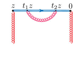
Figure 1: Self-energy-type correction for the gauge link.

Clearly, this correction is just a function of $z_{3}$. It does not induce any $\nu$-dependence, and the resulting $\nu$-independent factors cancel in the ratio (38). For this reason, the explicit form of this factor is not very essential in the pseudo-PDF approach.

For completeness, we present here the expression for the link self-energy digram in Feynman gauge obtained using the dimensional regularization,

$$-{g^{2}N_{c}\over 4\pi^{2}[(-z^{2}\mu_{\rm UV}^{2}+i\epsilon)]^{{d\over 2}-2}}{\Gamma\big{(}{d/2}-1\big{)}\over(3-d)(4-d)}G_{\mu\alpha}(z)G_{\lambda\beta}(0)\ ,$$ (2)

where the pole for $d=3$ ($d=4$) corresponds to the linear (logarithmic) UV divergences present in this diagram.

3.2 UV divergent vertex terms

UV divergent terms are also present in vertex diagrams involving gluons that connect the gauge link with the gluon lines, see Fig. 2. Clearly, the gluon exchange produces a correction just to one of the fields in the $G_{\mu\alpha}(z)\widetilde{G}_{\lambda\beta}(0)$ operator, while another remains intact. A minor complication compared to Refs. Balitsky:2019krf ; Balitsky:2021qsr is the presence of a dual field $\widetilde{G}$ in one of the vertices. But this changes only the tensor structure of the contributions without affecting the integral.

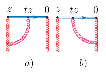
Figure 2: Vertex diagrams with gluons coming out of the gauge link.

As established in Refs. Balitsky:2019krf ; Balitsky:2021qsr , the vertex correction may be represented as the sum of the UV divergent and UV finite parts. The UV-divergent part of the vertex correction to $G_{\mu\alpha}(z)$ is given by

$$\frac{N_{c}g^{2}}{8\pi^{2}}\frac{\Gamma(d/2-1)}{(d-2)(-z^{2})^{d/2-1}}\int_{0}^{1}\differential u\,\left(u^{3-d}-u\right)\left(z_{\alpha}G_{z\mu}(\bar{u}z)-z_{\mu}G_{z\alpha}(\bar{u}z)\right)\ ,$$ (3)

where $G_{z\sigma}\equiv z^{\rho}G_{\rho\sigma}$ and $\bar{u}\equiv 1-u$. As we see, the overall $d$-dependent factor here is finite for $d=4$, but the $u$-integral diverges at the lower limit. If one uses the dimensional UV regularization with $d=4-2\varepsilon_{\rm UV}$, the divergence converts into a pole at $\varepsilon_{\rm UV}=0$. Isolating the UV divergence by taking $\bar{u}=1$ in the gluonic field produces

$$\frac{N_{c}g^{2}}{4\pi^{2}}\frac{\Gamma(d/2-1)}{(d-2)(-z^{2})^{d/2-1}}\left(\frac{1}{4-d}-\frac{1}{2}\right)\left(z_{\alpha}G_{z\mu}(z)-z_{\mu}G_{z\alpha}(z)\right)\$$ (4)

plus the remainder given by

$$\frac{N_{c}g^{2}}{8\pi^{2}}\frac{\Gamma(d/2-1)}{(d-2)(-z^{2})^{d/2-1}}\int_{0}^{1}\differential u\,\left[u^{3-d}-u\right]_{+(0)}\left(z_{\alpha}G_{z\mu}(\bar{u}z)-z_{\mu}G_{z\alpha}(\bar{u}z)\right)\ ,$$ (5)

where the plus-prescription at $u=0$ is defined as

$$\int_{0}^{1}\differential u\left[f(u)\right]_{+(0)}g(u)=\int_{0}^{1}\differential uf(u)[g(u)-g(0)]\ .$$ (6)

As explained in Refs. Balitsky:2019krf ; Balitsky:2021qsr , if we take $z=z_{3}$, the field ${\cal G}_{\mu\alpha}(z)=z_{\alpha}G_{z\mu}(z)-z_{\mu}G_{z\alpha}(z)$ in Eq. (4) is actually proportional to the field $G_{\mu\alpha}(z)$ in the original operator. In explicit form: ${\cal G}_{0i}(z)=0$, ${\cal G}_{ij}(z)=0$, ${\cal G}_{03}(z)=-z_{3}^{2}G_{03}(z)$ and ${\cal G}_{3i}(z)=-z_{3}^{2}G_{3i}(z)$. Thus, when one of the indices equals 3, we have a nontrivial vertex anomalous dimension (AD, call it $\gamma$), since ${\cal G}_{3\alpha}(z)=-z_{3}^{2}G_{3\alpha}(z)$ for all $\alpha$. In all other cases, we have a trivial (vanishing) vertex AD, since ${\cal G}_{ij}(z)=0$ and ${\cal G}_{0i}(z)=0$.

For the dual field $\widetilde{G}_{\lambda\beta}$, the “$\gamma$-counting” is inverse: if none of the indices $\lambda,\beta$ equals 3, the field has AD equal to $\gamma$. Otherwise, its AD is zero. Combining the ADs from $G$ and $\widetilde{G}$, we see that the matrix elements $\widetilde{M}_{0i;0i}$, $\widetilde{M}_{ij;ij}$, $\widetilde{M}_{03;03}$ and $\widetilde{M}_{3i;3i}$ all have vertex AD equal to $\gamma$; while $\widetilde{M}_{0i;3i}$ has zero AD and $\widetilde{M}_{3i;0i}$ has AD equal to $2\gamma$. These observations lead to the results announced in Section 2.6. Namely, the matrix element $\widetilde{M}_{ij;ij}$ has the same one-loop UV anomalous dimension as ${\widetilde{M}}_{0i;0i}$, while $\widetilde{M}_{30;03}$ has the same one-loop UV anomalous dimension as ${M}_{3i;3i}$.

Of course, the UV cut-off produced by the dimensional regularization is rather different from that produced by a finite lattice spacing. The latter, as pointed out earlier, is similar to the Polyakov regularization $1/z^{2}\to 1/(z^{2}-a^{2})$ for the gluon propagator in the coordinate space, with the parameter $a$ related to the lattice spacing by $a=a_{L}/\pi$. The UV logarithms $(\alpha_{s}N_{c}/4\pi)\ln z_{3}^{2}\mu^{2}_{\rm UV}$ in this case are substituted by $(\alpha_{s}N_{c}/4\pi)\ln(1+z_{3}^{2}/a^{2})$ (compare with Eq. (1)). In higher orders, they, as usual, exponentiate into

$$Z_{\rm L}(z_{3}/a_{L})=\left(1+\pi^{2}z_{3}^{2}/a_{L}^{2}\right)^{\alpha_{s}N_{c}/4\pi}\ .$$ (7)

For each particular type of the operator discussed above, one would have $Z^{\gamma}_{\rm L}(z_{3}/a_{L})$, where $\gamma$ is the number (0, or 1, or 2) corresponding to the operator in question.

Building the matching relations for particular matrix elements entering in the combinations listed in Eqs. (18), (22) and (24), we will need the following results for the UV-divergent parts of vertex corrections

$$G_{li}(z_{3})\widetilde{G}_{li}(0)\stackrel{{\scriptstyle\rm UV}}{{\longrightarrow}}\frac{g^{2}N_{c}\Gamma(d/2-1)}{4\pi^{2}(z_{3}^{2})^{d/2-2}}\int_{0}^{1}\differential u\left(\frac{u^{3-d}-u}{d-2}\right)G_{li}(\bar{u}z_{3})\widetilde{G}_{li}(0)\ ,$$ (8)

where $l=0,3$ or $l=j$ (in the latter case, also summation over $j$ is implied). We also have

$$G_{3i}(z_{3})\widetilde{G}_{0i}(0)\stackrel{{\scriptstyle\rm UV}}{{\longrightarrow}}\frac{g^{2}N_{c}\Gamma(d/2-1)}{2\pi^{2}(z_{3}^{2})^{d/2-2}}\int_{0}^{1}\differential u\left(\frac{u^{3-d}-u}{d-2}\right)G_{3i}(\bar{u}z_{3})\widetilde{G}_{0i}(0)$$ (9)

and $G_{0i}(z_{3})\widetilde{G}_{3i}(0)\stackrel{{\scriptstyle\rm UV}}{{\longrightarrow}}0$.

3.3 Evolution contribution from the vertex diagrams

The UV finite contribution from the vertex diagrams shown in Fig. 2 generates the evolution $z_{3}^{2}$-dependence of the matrix element. It may be symbolically written as

$$G_{\mu\alpha}(z_{3})\widetilde{G}_{\lambda\beta}(0)\stackrel{{\scriptstyle\rm Evol}}{{\longrightarrow}}\frac{g^{2}N_{c}\Gamma(d/2-2)}{4\pi^{2}(z_{3}^{2})^{d/2-2}}\int_{0}^{1}\differential u\left[\frac{u^{3-d}-1}{d-3}\right]_{+}G_{\mu\alpha}(\bar{u}z_{3})\widetilde{G}_{\lambda\beta}(0)\ .$$ (10)

In this case, the gluonic operator has the same tensor structure as the original operator $G_{\mu\alpha}(z_{3})\widetilde{G}_{\lambda\beta}(0)$ differing from it just by rescaling $z\to\bar{u}z$. There is no mixing with operators of a different type. Also, the evolution factor is the same for any combination of the indices in $G_{\mu\alpha}\widetilde{G}_{\lambda\beta}$.

The $u$-integral now does not diverge for $d=4$, but the overall $\Gamma(d/2-2)$ factor has a pole $1/(d-4)$. Note that the singularity for $d=3$ from the pole $1/(d-3)$ formally corresponds to a linear UV divergence. However, it is compensated by a zero coming for $d=3$ from the $\left[u^{3-d}-1\right]$ combination in the integrand. The remaining $1/(d-4)$ pole corresponds to a collinear divergence that appears because all the propagators and external lines correspond to massless particles. The integrand factor $\left[u^{3-d}-1\right]_{+}$ for $d=4$ produces the $\left[\bar{u}/u\right]_{+}$ part of the evolution kernel.

3.4 Gluon self-energy diagrams

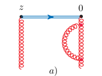
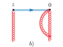
Figure 3: Gluon self-energy-type insertions into the right leg.

Another simple type of one-loop corrections is represented by the gluon self-energy diagrams, one of which is shown in Fig. 3a. These diagrams have both the UV and collinear divergences. The combined contribution of the Fig. 3 diagrams and their left-leg analogs is given by

$${g^{2}N_{c}\over 8\pi^{2}}\frac{1}{2-d/2}\left[2-\frac{\beta_{0}}{2N_{c}}\right]G_{\mu\alpha}(z)G_{\lambda\beta}(0)\ ,$$ (11)

where $\beta_{0}=11N_{c}/3$ in gluodynamics, so that the terms in the square bracket combine into 1/6.

3.5 Box diagram

The most nontrivial is the calculation of the “box” diagram corresponding to a gluon exchange between two gluon lines (see Fig. 4). While this diagram has no UV divergences, it contains DGLAP $\log z_{3}^{2}$ evolution contributions. In distinction to the vertex diagrams, the original $G_{\mu\alpha}(z)G_{\nu\beta}(0)$ operator generates in this case a mixture of various bilocal operators in which $G_{\mu\alpha}(uz)G_{\nu\beta}(0)$ is projected onto the structures built from the metric tensor $g$ and the vectors $p$ and $z$.

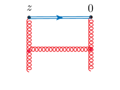
Figure 4: Box diagram.

The results for arbitrary indices $\sigma\rho\mu\lambda$ are given below. We present them in the operator form, however, the operators that have the form of a full derivative are abandoned. In other words, we keep only those operators that survive in the forward matrix element.

The full result for the box correction to the forward matrix element of the $G_{\sigma\rho}\widetilde{G}_{\mu\lambda}$ operator may be represented by a sum of three terms. The first one has $\Gamma(d/2)$ as an overall factor.

$$G_{\sigma\rho}(z)\widetilde{G}_{\mu\lambda}(0)\stackrel{{\scriptstyle\rm Box,1}}{{\longrightarrow}}\frac{g^{2}N_{c}\Gamma(d/2)}{4\pi^{2}\left(z_{3}^{2}\right)^{d/2}}\left(\epsilon_{\sigma\rho\mu z}z_{\lambda}-\epsilon_{\sigma\rho\lambda z}z_{\mu}\right)\int_{0}^{1}\differential u\frac{\bar{u}^{3}}{3}G_{z\xi}(uz)G_{z}^{\ \xi}(0)+\ldots\ .$$ (12)

On the right-hand side here and in the next two equations we omit terms containing an extra ${\cal O}(z^{2})$ factor, operators with $D_{\nu}G^{\mu\nu}$ or with more than two gluon fields.

The second term is proportional to $\Gamma(d/2-1)$

$$G_{\sigma\rho}(z)\widetilde{G}_{\mu\lambda}(0)\stackrel{{\scriptstyle\rm Box,2}}{{\longrightarrow}}\frac{g^{2}N_{c}\Gamma(d/2-1)}{8\pi^{2}\left(z_{3}^{2}\right)^{d/2-1}}\int_{0}^{1}\differential u\left\{\vphantom{\frac{1}{2}}\epsilon_{\sigma\rho\mu\lambda}\frac{\bar{u}^{3}}{3}G_{z\xi}(uz)G_{z}^{\ \xi}(0)\right.$$

$$\quad\left.-\frac{\bar{u}^{3}}{3}\epsilon_{\sigma\rho\lambda}^{\ \ \ \ \nu}G_{z\nu}(uz)G_{z\mu}(0)\right.\left.-\left(2u\bar{u}+\frac{\bar{u}^{3}}{3}\right)\epsilon_{\sigma\rho\lambda}^{\ \ \ \ \nu}G_{z\mu}(uz)G_{z\nu}(0)\right.$$

$$\quad+\bar{u}^{2}\left(\vphantom{\frac{1}{2}}\right.\epsilon_{\sigma\rho z}^{\ \ \ \ \eta}G_{\lambda\eta}(uz)G_{z\mu}(0)-\epsilon_{\sigma\rho}^{\ \ \ \nu\eta}z_{\mu}G_{z\nu}(uz)G_{\lambda\eta}(0)\left.\vphantom{\frac{1}{2}}\right)$$

$$\quad+\bar{u}(1+u)\left(\vphantom{\frac{1}{2}}\right.\epsilon_{\sigma\rho z}^{\ \ \ \ \eta}G_{z\mu}(uz)G_{\lambda\eta}(0)-\epsilon_{\sigma\rho}^{\ \ \ \nu\eta}z_{\mu}G_{\lambda\eta}(uz)G_{z\nu}(0)\left.\vphantom{\frac{1}{2}}\right)$$

$$\quad+\left(\frac{\bar{u}^{2}}{2}-\frac{\bar{u}^{3}}{3}\right)\left(\vphantom{\frac{1}{2}}\right.\epsilon_{\sigma\rho z\lambda}\Big{(}G_{\mu\xi}(uz)G_{z}^{\ \xi}(0)+G_{z\xi}(uz)G_{\mu}^{\ \xi}(0)\Big{)}$$

$$\quad\hskip 71.13188pt-\epsilon_{\sigma\rho\lambda}^{\ \ \ \ \nu}z_{\mu}\Big{(}G_{\nu\xi}(uz)G_{z}^{\ \xi}(0)+G_{z\xi}(uz)G_{\nu}^{\ \xi}(0)\Big{)}\left.\vphantom{\frac{1}{2}}\right)$$

$$\quad+2\bar{u}\epsilon_{\sigma\rho z}^{\ \ \ \ \eta}z_{\mu}G_{\lambda\xi}(uz)G_{\eta}^{\ \xi}(0)\left.-\frac{\bar{u}^{3}}{6}\epsilon_{\sigma\rho z\lambda}z_{\mu}G_{\eta\xi}(uz)G^{\eta\xi}(0)\right\}\ -\{\lambda\leftrightarrow\mu\}\ +\ldots\ .$$ (13)

The third term is proportional to $\Gamma(d/2-2)$:

$$G_{\sigma\rho}(z)\widetilde{G}_{\mu\lambda}(0)\stackrel{{\scriptstyle\rm Box,3}}{{\longrightarrow}}\frac{1}{2}\epsilon_{\sigma\rho}^{\ \ \nu\eta}\frac{g^{2}N_{c}\Gamma(d/2-2)}{8\pi^{2}\left(z_{3}^{2}\right)^{d/2-2}}\int_{0}^{1}\differential u\left\{\vphantom{\frac{1}{2}}\right.-2\bar{u}G_{\lambda\eta}(uz)G_{\mu\nu}(0)$$

$$-uG_{\mu\lambda}(uz)G_{\nu\eta}(0)+\bar{u}(1/2-u)G_{\nu\eta}(uz)G_{\mu\lambda}(0)+\bar{u}(1/2+u)G_{\mu\lambda}(uz)G_{\nu\eta}(0)$$

$$+{\bar{u}u^{2}}g_{\lambda\eta}\left(G_{\mu\xi}(uz)G_{\nu}^{\ \xi}(0)+G_{\nu\xi}(uz)G_{\mu}^{\ \xi}(0)\right)+\bar{u}\left(g_{\mu\nu}G_{\lambda\xi}(uz)G_{\eta}^{\ \xi}(0)-g_{\mu\eta}G_{\lambda\xi}(uz)G_{\nu}^{\ \xi}(0)\right)$$

$$\hskip 110.96574pt-\frac{\bar{u}^{3}}{6}g_{\mu\nu}g_{\lambda\eta}G_{\zeta\xi}(uz)G^{\zeta\xi}(0)\left.\vphantom{\frac{1}{2}}\right\}-\{\lambda\leftrightarrow\mu\}\ +\ldots\ .$$ (14)

We use here the notation $\epsilon_{z\alpha\beta\gamma}=z^{\mu}\epsilon_{\mu\alpha\beta\gamma}$, etc.

In practice, however, one may only need the projections of these expressions onto particular combinations of indices corresponding to matrix elements $\widetilde{M}_{0i;0i}+\widetilde{M}_{ij;ij}$, $\widetilde{M}_{3i;3i}-\widetilde{M}_{ij;ij}$, $\widetilde{M}_{0i;3i}$ and $\widetilde{M}_{3i;0i}$ that contain the “twist-2” invariant amplitude $\widetilde{\mathcal{M}}_{ps}^{(+)}-\nu\widetilde{\mathcal{M}}_{pp}$ and are listed in Eqs. (18), (22), (23) and (24).

4 Matching relations

As discussed already, the sum $\widetilde{M}_{00}\equiv\widetilde{M}_{0i;0i}+\widetilde{M}_{ij;ij}$ contains only the invariant amplitudes $\widetilde{\mathcal{M}}_{sp}^{(+)}$ and $\widetilde{\mathcal{M}}_{pp}$ entering in the “twist-2” combination $\widetilde{\mathcal{M}}_{sp}^{(+)}-\nu\widetilde{\mathcal{M}}_{pp}$ . Moreover, since

$$\widetilde{M}_{00}=-2p_{3}p_{0}\left[\widetilde{\mathcal{M}}_{sp}^{(+)}-\nu\widetilde{\mathcal{M}}_{pp}-\nu\widetilde{\mathcal{M}}_{pp}m^{2}/p_{3}^{2}\right]\ ,$$ (15)

the ratio $\widetilde{M}_{00}/(-2p_{3}p_{0})$ tends to $\widetilde{\mathcal{M}}_{sp}^{(+)}-\nu\widetilde{\mathcal{M}}_{pp}$ for large $p_{3}$ at fixed $\nu$. Other combinations of matrix elements, namely, (22), (23) and (24), contain extra “contaminating” invariant amplitudes, like $\widetilde{\mathcal{M}}_{sz}^{(+)}$, $\widetilde{\mathcal{M}}_{pz}^{(+)}$, $\widetilde{\mathcal{M}}_{zz}$, etc. For this reason, the combination $\widetilde{M}_{0i;0i}+\widetilde{M}_{ij;ij}$ is the primary object of the ongoing lattice studies of the polarized gluon distribution.

4.1 Total one-loop correction

Combining all the one-loop corrections for the relevant operator (assuming that it is inserted into a forward matrix element $\langle\ldots\rangle$) we get

$$\langle G_{0i} (z)\widetilde{G}_{0i}(0)+G_{ij}(z)\widetilde{G}_{ij}(0)\rangle$$

$$\to \frac{g^{2}N_{c}}{8\pi^{2}}\left[{4\over 3}\left(\frac{1}{\epsilon_{\text{UV}}}+\log\left(z_{3}^{2}\mu^{2}\frac{e^{2\gamma_{E}}}{4}\right)\right)+2\right]\left\langle G_{0i}(z)\widetilde{G}_{0i}(0)+G_{ij}(z)\widetilde{G}_{ij}(0)\right\rangle$$

$$+\frac{g^{2}N_{c}}{8\pi^{2}}\int_{0}^{1}\differential u\left({1\over\bar{u}}-\bar{u}\right)_{+}\left\langle G_{0i}(uz)\widetilde{G}_{0i}(0)+G_{ij}(uz)\widetilde{G}_{ij}(0)\right\rangle$$

$$+\frac{g^{2}N_{c}}{8\pi^{2}}\int_{0}^{1}\differential u\left\{\vphantom{\frac{1}{2}}\right.\bar{u}^{2}\left\langle G_{0i}(uz)\widetilde{G}_{0i}(0)+G_{ij}(uz)\widetilde{G}_{ij}(0)\right\rangle$$

$$-\bar{u}(1+u)\left\langle G_{3i}(uz)\widetilde{G}_{3i}(0)+2G_{30}(uz)\widetilde{G}_{30}(0)\right\rangle\left.\vphantom{\frac{1}{2}}\right\}$$

$$+\frac{g^{2}N_{c}}{8\pi^{2}}\int_{0}^{1}\differential u\left(\left(\frac{1}{\epsilon_{IR}}-\log\left(z_{3}^{2}\mu^{2}\frac{e^{2\gamma_{E}}}{4}\right)\right)\left(2\bar{u}u+2\left[\frac{u}{\bar{u}}-u\right]_{+}+{1\over 2}\left({\beta_{0}\over N_{c}}-6\right)\delta(\bar{u})\right)\right.$$

$$\left.-\left[\frac{4u}{\bar{u}}+\frac{4\log(1-u)}{\bar{u}}\right]_{+}\right)\left\langle G_{0i}(uz)\widetilde{G}_{0i}(0)+G_{ij}(uz)\widetilde{G}_{ij}(0)\right\rangle$$

$$+\frac{g^{2}N_{c}}{8\pi^{2}}\left(\frac{1}{\epsilon_{IR}}-\log\left(z_{3}^{2}\mu^{2}\frac{e^{2\gamma_{E}}}{4}\right)\right)\int_{0}^{1}\differential u\,2\bar{u}u\left\langle G_{3i}(uz)\widetilde{G}_{3i}(0)+2G_{30}(uz)\widetilde{G}_{30}(0)\right\rangle$$ (16)

Using the relations in Eqs. (27) and (30) we change $\langle G_{3i}(uz)\widetilde{G}_{3i}(0)+2G_{30}(uz)\widetilde{G}_{30}(0)\rangle$ into $\langle G_{0i}(uz)\widetilde{G}_{0i}(0)+G_{ij}(uz)\widetilde{G}_{ij}(0)\rangle$ and write everything in terms of the latter. Switching to matrix elements, we get

$${\widetilde{M}}_{0i;0i}(z,p)+{\widetilde{M}}_{ij;ij}(z,p)$$

$$\to\frac{g^{2}N_{c}}{8\pi^{2}}\left[{4\over 3}\left(\frac{1}{\epsilon_{\text{UV}}}+\log\left(z_{3}^{2}\mu^{2}\frac{e^{2\gamma_{E}}}{4}\right)\right)+2\right]\left({\widetilde{M}}_{0i;0i}(z,p)+{\widetilde{M}}_{ij;ij}(z,p)\right)$$

$$\quad+\frac{g^{2}N_{c}}{8\pi^{2}}\int_{0}^{1}\differential u\left\{-2\bar{u}u+\left({1\over\bar{u}}-\bar{u}\right)_{+}-4\left[\frac{u+\log(1-u)}{\bar{u}}\right]_{+}\right.$$

$$\quad\left.+\left(\frac{1}{\epsilon_{IR}}-\log\left(z_{3}^{2}\mu^{2}\frac{e^{2\gamma_{E}}}{4}\right)\right)\left[\left\{4u\bar{u}+2\left[u^{2}/\bar{u}\right]_{+}\right\}+{1\over 2}\left({\beta_{0}\over N_{c}}-6\right)\delta(\bar{u})\right]\right\}$$

$$\quad\times\left({\widetilde{M}}_{0i;0i}(uz,p)+{\widetilde{M}}_{ij;ij}(uz,p)\right)\ .$$ (17)

4.2 Gluon-quark mixing

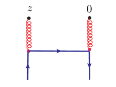
Figure 5: Gluon-quark mixing diagram.

In addition to the gluon-gluon transitions, we also need to include the contribution from gluon-quark mixing. The result that correspons to ${\widetilde{M}}_{0i;0i}+{\widetilde{M}}_{ij;ij}$ in the $\overline{\rm MS}$ scheme at the operator level is:

$$-\frac{g^{2}C_{F}}{8\pi^{2}}\int_{0}^{1}\differential u~{}2\bar{u}u\,\partial_{0}\mathcal{O}_{q}^{0}\left(uz\right)-\frac{g^{2}C_{F}}{8\pi^{2}}\log\left(z_{3}^{2}\mu^{2}{e^{2\gamma_{E}}\over 4}\right)\int_{0}^{1}\differential u\left(1-\bar{u}^{2}\right)\partial_{0}\mathcal{O}_{q}^{0}\left(uz\right).$$ (18)

The singlet combination of quark fields is defined as

$$\mathcal{O}_{q}^{0}\left(z\right) ={1\over 2}\sum_{f}\left(\bar{\psi}_{f}(z)\gamma^{0}\gamma_{5}\psi_{f}(0)+\bar{\psi}_{f}(0)\gamma^{0}\gamma_{5}\psi_{f}(z)\right),$$ (19)

with $f$ numerating quark flavors. Since $\mathcal{O}_{q}^{0}$ is even in $z$, the matrix element can be parametrized by

$$\bra{p,s}\mathcal{O}_{q}^{0}\left(z\right)\ket{p,s} =-\,2ip_{3}\int_{0}^{1}\differential x\cos\left(xpz\right)\Delta f_{S}\left(x\right).$$ (20)

Then, applying the time derivative, we have:

$$\partial_{0}\bra{p,s}\mathcal{O}_{q}^{0}\left(z\right)\ket{p,s}=-\,2p_{0}p_{3}\,i\Delta\mathcal{I}_{S}\left(\nu\right),$$ (21)

where $\nu=-(zp)$, as usual, and

$$\Delta\mathcal{I}_{S}\left(\nu\right) =\int_{0}^{1}x\sin\left(x\nu\right)\Delta f_{S}\left(x\right).$$ (22)

Applying this parametrization to Eq. (18), we obtain:

$$\bra{p,s} G_{0i}\left(z\right)\widetilde{G}_{0i}\left(0\right)\ket{p,s}+\bra{p,s}G_{ij}\left(z\right)\widetilde{G}_{ij}\left(0\right)\ket{p,s}$$

$$\to 2p_{0}p_{3}\frac{g^{2}C_{F}}{8\pi^{2}}\int_{0}^{1}\differential u\left[\log\left(z_{3}^{2}\mu^{2}{e^{2\gamma_{E}}\over 4}\right)\widetilde{\cal B}_{gq}(u)+2\bar{u}u\right]i\Delta\mathcal{I}_{S}\left(u\nu\right),$$ (23)

with the $gq$ component of the evolution kernel given by $\widetilde{\cal B}_{gq}(u)=1-(1-u)^{2}$.

4.3 Building reduced Ioffe-time pseudodistribution

A disadvantage of $\widetilde{M}_{00}(z_{3},p_{3})$ is that it is proportional to $p_{3}$ for small momenta $p_{3}$, and one cannot use $\widetilde{M}_{00}(z_{3},p_{3}=0)$ in the denominator of the ratio defining the reduced pseudo-ITD, like it is done in Eq. (38). To overcome this difficulty, we propose to form the ratio of $\widetilde{M}_{00}(z_{3},p_{3})$ and the $p_{3}=0$ value of the unpolarized matrix element $M_{00}\equiv{M}_{0i;i0}+{M}_{ij;ji}$ of the operator ${G}_{0i}G_{i0}+{G}_{ij}G_{ji}$ discussed in Ref.Balitsky:2019krf . As established there, at the tree level, $M_{00}(z_{3},p_{3})=2p_{0}^{2}\mathcal{M}_{pp}(\nu,z_{3}^{2})$, with the invariant amplitude ${\mathcal{M}}_{pp}(\nu,z_{3}^{2})$ being proportional to the pseudo-ITD for the unpolarized gluon density $xf_{g}(x)$ divided by $\langle x_{g}\rangle$. Thus, we are going to consider the pseudo-ITD $\widetilde{\mathfrak{M}}\left(\nu,z_{3}^{2}\right)$ defined by

$$\widetilde{\mathfrak{M}}\left(\nu,z_{3}^{2}\right)\equiv i\frac{\{\widetilde{M}_{00}\left(z_{3},p_{3}\right)/p_{3}p_{0}\}/Z_{\rm L}(z_{3}/a_{L})}{\{{M}_{00}\left(z_{3},p_{3}=0\right)/m^{2}\}}~{}.$$ (24)

The factor $i$ is included in view of Eq. (7), and the factor $1/Z_{\rm L}(z_{3}/a_{L})$ (defined by Eq. (7)) is introduced to cancel the UV logarithmic vertex AD of the $\widetilde{M}_{00}$ matrix element.

As we discussed, the main reason for taking the ratio is to cancel the factor $Z_{\rm lin}(z_{3}^{2}/a^{2})$ generated by linear divergence in the gluon-link self-energy. This factor is the same in $\widetilde{M}_{00}\left(z_{3},p_{3}\right)$ and in ${M}_{00}\left(z_{3},p_{3}=0\right)$, so this factor cancels in the ratio. Furthermore, the denominator factor does not have DGLAP evolution logarithms, hence the DGLAP structure of $\widetilde{\mathfrak{M}}\left(\nu,z_{3}^{2}\right)$ is determined by DGLAP logarithms of the numerator factor $\widetilde{M}_{00}\left(z_{3},p_{3}\right)$.

Using the results of our calculations for the one-loop corrections to the combinations ${\widetilde{M}}_{0i;0i}(z,p)+{\widetilde{M}}_{ij;ij}(z,p)$ and ${M}_{0i;i0}(z_{3},p_{3}=0)+{M}_{ij;ji}(z_{3},p_{3}=0)$, and neglecting the additional term in Eq. (21) with factor $z_{3}^{2}/\nu$, we obtain the matching relation

$$\widetilde{\mathfrak{M}}\left(\nu,z_{3}^{2}\right)\langle x_{g}\rangle_{\mu^{2}} ={{\cal I}_{p}(\nu,\mu^{2})}-\frac{\alpha_{s}N_{c}}{2\pi}\int_{0}^{1}\differential u\,{{\cal I}_{p}(u\nu,\mu^{2})}\left\{\log\left(z_{3}^{2}\mu^{2}\frac{e^{2\gamma_{E}}}{4}\right)\right.$$

$$\left.\left(\left[{2u^{2}\over\bar{u}}+4u\bar{u}\right]_{+}-\left(\frac{1}{2}+\frac{4}{3}{\langle x_{S}\rangle_{\mu^{2}}\over\langle x_{g}\rangle_{\mu^{2}}}\right)\delta(\bar{u})\right)\right.$$

$$\quad\left.+4\left[\frac{u+\log(1-u)}{\bar{u}}\right]_{+}-\left({1\over\bar{u}}-\bar{u}\right)_{+}-\frac{1}{2}\delta(\bar{u})+2\bar{u}u\right\}$$

$$\quad-\frac{\alpha_{s}C_{F}}{2\pi}\int_{0}^{1}\differential u\,{\Delta\mathcal{I}_{S}\left(u\nu,\mu^{2}\right)}\left\{\log\left(z_{3}^{2}\mu^{2}{e^{2\gamma_{E}}\over 4}\right)\widetilde{\cal B}_{gq}(u)+2\bar{u}u\right\}$$ (25)

between the “lattice function” $\widetilde{\mathfrak{M}}(\nu,z_{3}^{2})$ and the polarized light-cone ITDs for gluons ${\cal I}_{p}(\nu,\mu^{2})$ and for quarks $\Delta\mathcal{I}_{S}\left(\nu,\mu^{2}\right)$. The factor

$$\langle x_{g}\rangle_{\mu^{2}}\equiv\int_{0}^{1}\differential x\,xf_{g}(x,\mu^{2})$$ (26)

has the meaning of the fraction of the hadron momentum carried by the gluons, while

$$\langle x_{S}\rangle_{\mu^{2}}\equiv\sum_{f}\int_{0}^{1}\differential x\,x\left(f_{f}(x,\mu^{2})+f_{\bar{f}}(x,\mu^{2})\right)$$ (27)

corresponds to the fraction of the hadron momentum carried by the singlet quarks. Note that $\left[{2u^{2}/\bar{u}}+4u\bar{u}\right]_{+}$ coincides for $u\neq 1$ with the $gg$-part of the Altarelli-Parisi kernel for polarized gluon distribution $x\Delta g(x,\mu^{2})$ (see, e.g., Ref. Balitsky:1997mj ).

Eq. (25) allows one to extract just the shape of the polarized gluon distribution. Its normalization, i.e., the magnitude of $\langle x_{g}\rangle_{\mu^{2}}$ must be taken from an independent lattice calculation, similar to that performed in Ref. Yang:2018bft . The singlet quark function $\Delta{\cal I}_{S}(w\nu,\mu^{2})$ that appears in the ${\cal O}(\alpha_{s})$ correction and $\langle x_{S}\rangle_{\mu^{2}}$ should be also calculated (or estimated) independently.

Using Eq. (9) allows us to write (25) directly in terms of the LC polarized gluon distribution:

$$~{}\widetilde{\mathfrak{M}}\left(\nu,z_{3}^{2}\right)= \int_{0}^{1}\differential x{x\Delta g(x,\mu^{2})\over\expectationvalue{x_{g}}_{\mu^{2}}}\widetilde{R}_{gg}\left(x\nu,z_{3}^{2}\mu^{2}\right)$$

$$+\int_{0}^{1}\differential x{x\Delta f_{S}(x,\mu^{2})\over\expectationvalue{x_{g}}_{\mu^{2}}}\widetilde{R}_{gq}\left(x\nu,z_{3}^{2}\mu^{2}\right),$$ (28)

where the gluon-gluon kernel $\widetilde{R}_{gg}$ is given by

$$\widetilde{R}_{gg}\left(x\nu,z_{3}^{2}\mu^{2}\right)=\sin(x\nu)- \frac{g^{2}N_{c}}{8\pi^{2}}\int_{0}^{1}\differential u\sin(ux\nu)\left\{\log\left(z_{3}^{2}\mu^{2}\frac{e^{2\gamma_{E}}}{4}\right)\right.$$

$$\left.\left(\left[{2u^{2}\over\bar{u}}+4u\bar{u}\right]_{+}-\left(\frac{1}{2}+\frac{4}{3}{\langle x_{S}\rangle_{\mu^{2}}\over\langle x_{g}\rangle_{\mu^{2}}}\right)\delta(\bar{u})\right)\right.$$

$$\quad\left.+4\left[\frac{u+\log(1-u)}{\bar{u}}\right]_{+}-\left({1\over\bar{u}}-\bar{u}\right)_{+}-\frac{1}{2}\delta(\bar{u})+2\bar{u}u\right\},$$ (29)

and the gluon-quark kernel $\widetilde{R}_{gq}$ is

$$\widetilde{R}_{gq} \left(x\nu,z_{3}^{2}\mu^{2}\right)$$

$$= -\frac{\alpha_{s}C_{F}}{2\pi}\int_{0}^{1}\differential u\sin(ux\nu)\left\{\log\left(z_{3}^{2}\mu^{2}{e^{2\gamma_{E}}\over 4}\right)\widetilde{\cal B}_{gq}(u)+2\bar{u}u\right\}.$$ (30)

5 Summary

In this paper, we formulated the basic points of the pseudo-PDF approach to lattice calculation of polarized gluon PDFs. In particular, we have presented the results of our calculations of the one-loop corrections for the bilocal $G_{\mu\alpha}(z)\widetilde{G}_{\lambda\beta}(0)$ correlator of gluonic fields. We gave the expressions for a general situation when all four indices are arbitrary, and also specified them for combinations of indices giving three matrix elements that contain the structures corresponding to twist-2 invariant amplitude related to the polarized PDF. We have studied the evolution properties of these matrix elements, and derived matching relations between Euclidean and light-cone Ioffe-time distributions that are necessary for extraction of the polarized gluon distributions from the lattice data.

Acknowledgements. We thank K. Orginos, J.-W. Qiu, D. Richards, R. Sufian and T. Khan for interest in our work and discussions. This work is supported by Jefferson Science Associates, LLC under U.S. DOE Contract #DE-AC05-06OR23177 and by U.S. DOE Grant #DE-FG02-97ER41028.

References

- (1) M. Constantinou et al., Parton distributions and lattice-QCD calculations: Toward 3D structure, Prog. Part. Nucl. Phys. 121 (2021) 103908, [2006.08636].
- (2) K. Cichy and M. Constantinou, A guide to light-cone PDFs from Lattice QCD: an overview of approaches, techniques and results, Adv. High Energy Phys. 2019 (2019) 3036904, [1811.07248].
- (3) X. Ji, Parton Physics on a Euclidean Lattice, Phys. Rev. Lett. 110 (2013) 262002, [1305.1539].
- (4) X. Ji, Parton Physics from Large-Momentum Effective Field Theory, Sci. China Phys. Mech. Astron. 57 (2014) 1407–1412, [1404.6680].
- (5) Y.-Q. Ma and J.-W. Qiu, Extracting Parton Distribution Functions from Lattice QCD Calculations, Phys. Rev. D 98 (2018) 074021, [1404.6860].
- (6) Y.-Q. Ma and J.-W. Qiu, Exploring Partonic Structure of Hadrons Using ab initio Lattice QCD Calculations, Phys. Rev. Lett. 120 (2018) 022003, [1709.03018].
- (7) A. V. Radyushkin, Quasi-parton distribution functions, momentum distributions, and pseudo-parton distribution functions, Phys. Rev. D 96 (2017) 034025, [1705.01488].
- (8) A. Radyushkin, Quasi-PDFs and pseudo-PDFs, PoS QCDEV2017 (2017) 021, [1711.06031].
- (9) K. Orginos, A. Radyushkin, J. Karpie and S. Zafeiropoulos, Lattice QCD exploration of parton pseudo-distribution functions, Phys. Rev. D 96 (2017) 094503, [1706.05373].
- (10) V. Braun and D. Müller, Exclusive processes in position space and the pion distribution amplitude, Eur. Phys. J. C 55 (2008) 349–361, [0709.1348].
- (11) G. S. Bali et al., Pion distribution amplitude from Euclidean correlation functions, Eur. Phys. J. C 78 (2018) 217, [1709.04325].
- (12) G. S. Bali, V. M. Braun, B. Gläßle, M. Göckeler, M. Gruber, F. Hutzler et al., Pion distribution amplitude from Euclidean correlation functions: Exploring universality and higher-twist effects, Phys. Rev. D 98 (2018) 094507, [1807.06671].
- (13) X. Xiong, X. Ji, J.-H. Zhang and Y. Zhao, One-loop matching for parton distributions: Nonsinglet case, Phys. Rev. D 90 (2014) 014051, [1310.7471].
- (14) X. Ji and J.-H. Zhang, Renormalization of quasiparton distribution, Phys. Rev. D 92 (2015) 034006, [1505.07699].
- (15) T. Izubuchi, X. Ji, L. Jin, I. W. Stewart and Y. Zhao, Factorization Theorem Relating Euclidean and Light-Cone Parton Distributions, Phys. Rev. D 98 (2018) 056004, [1801.03917].
- (16) W. Wang and S. Zhao, On the power divergence in quasi gluon distribution function, JHEP 05 (2018) 142, [1712.09247].
- (17) W. Wang, S. Zhao and R. Zhu, Gluon quasidistribution function at one loop, Eur. Phys. J. C 78 (2018) 147, [1708.02458].
- (18) W. Wang, J.-H. Zhang, S. Zhao and R. Zhu, Complete matching for quasidistribution functions in large momentum effective theory, Phys. Rev. D 100 (2019) 074509, [1904.00978].
- (19) X. Ji, A. Schäfer, X. Xiong and J.-H. Zhang, One-Loop Matching for Generalized Parton Distributions, Phys. Rev. D 92 (2015) 014039, [1506.00248].
- (20) X. Xiong and J.-H. Zhang, One-loop matching for transversity generalized parton distribution, Phys. Rev. D 92 (2015) 054037, [1509.08016].
- (21) Y.-S. Liu, W. Wang, J. Xu, Q.-A. Zhang, J.-H. Zhang, S. Zhao et al., Matching generalized parton quasidistributions in the RI/MOM scheme, Phys. Rev. D 100 (2019) 034006, [1902.00307].
- (22) X. Ji, J.-H. Zhang and Y. Zhao, More On Large-Momentum Effective Theory Approach to Parton Physics, Nucl. Phys. B 924 (2017) 366–376, [1706.07416].
- (23) A. V. Radyushkin, Quark pseudodistributions at short distances, Phys. Lett. B 781 (2018) 433–442, [1710.08813].
- (24) A. Radyushkin, One-loop evolution of parton pseudo-distribution functions on the lattice, Phys. Rev. D 98 (2018) 014019, [1801.02427].
- (25) J.-H. Zhang, J.-W. Chen and C. Monahan, Parton distribution functions from reduced Ioffe-time distributions, Phys. Rev. D 97 (2018) 074508, [1801.03023].
- (26) A. V. Radyushkin, Generalized parton distributions and pseudodistributions, Phys. Rev. D 100 (2019) 116011, [1909.08474].
- (27) I. Balitsky, W. Morris and A. Radyushkin, Gluon Pseudo-Distributions at Short Distances: Forward Case, Phys. Lett. B 808 (2020) 135621, [1910.13963].
- (28) I. Balitsky, W. Morris and A. Radyushkin, Gluon pseudo-distributions at short distances, in 28th International Workshop on Deep Inelastic Scattering and Related Subjects, 6, 2021, 2106.01916.
- (29) I. Balitsky, W. Morris and A. Radyushkin, Short-Distance Structure of Unpolarized Gluon Pseudodistributions, 2111.06797.
- (30) Z. Fan, R. Zhang and H.-W. Lin, Nucleon gluon distribution function from 2 + 1 + 1-flavor lattice QCD, Int. J. Mod. Phys. A 36 (2021) 2150080, [2007.16113].
- (31) Z. Fan and H.-W. Lin, Gluon parton distribution of the pion from lattice QCD, Phys. Lett. B 823 (2021) 136778, [2110.14471].
- (32) HadStruc collaboration, T. Khan et al., Unpolarized gluon distribution in the nucleon from lattice quantum chromodynamics, Phys. Rev. D 104 (2021) 094516, [2107.08960].
- (33) A. Radyushkin and S. Zhao, One-loop structure of parton distribution for the gluon condensate and “zero modes”, JHEP 12 (2021) 010, [2111.00887].
- (34) A. V. Manohar, Polarized parton distribution functions, Phys. Rev. Lett. 66 (1991) 289–292.
- (35) V. Braun, P. Gornicki and L. Mankiewicz, Ioffe - time distributions instead of parton momentum distributions in description of deep inelastic scattering, Phys. Rev. D 51 (1995) 6036–6051, [hep-ph/9410318].
- (36) Z.-Y. Li, Y.-Q. Ma and J.-W. Qiu, Multiplicative Renormalizability of Operators defining Quasiparton Distributions, Phys. Rev. Lett. 122 (2019) 062002, [1809.01836].
- (37) J.-H. Zhang, X. Ji, A. Schäfer, W. Wang and S. Zhao, Accessing Gluon Parton Distributions in Large Momentum Effective Theory, Phys. Rev. Lett. 122 (2019) 142001, [1808.10824].
- (38) I. I. Balitsky and V. M. Braun, Evolution Equations for QCD String Operators, Nucl. Phys. B 311 (1989) 541–584.
- (39) J.-W. Chen, X. Ji and J.-H. Zhang, Improved quasi parton distribution through Wilson line renormalization, Nucl. Phys. B 915 (2017) 1–9, [1609.08102].
- (40) I. I. Balitsky and A. V. Radyushkin, Light ray evolution equations and leading twist parton helicity dependent nonforward distributions, Phys. Lett. B 413 (1997) 114–121, [hep-ph/9706410].
- (41) Y.-B. Yang, M. Gong, J. Liang, H.-W. Lin, K.-F. Liu, D. Pefkou et al., Nonperturbatively renormalized glue momentum fraction at the physical pion mass from lattice QCD, Phys. Rev. D 98 (2018) 074506, [1805.00531].