Quasinormal mode analysis of chiral power flow from linearly polarized dipole emitters coupled to index-modulated microring resonators close to an exceptional point

Abstract

Chiral emission can be achieved from a circularly polarized dipole emitter in a nanophotonic structure that possess special polarization properties such as a polarization singularity, namely with right or left circularly polarization (C-points). Recently, Chen et. al. [Nature Physics 16, 571 (2020)] demonstrated the surprising result of chiral radiation from a linearly-polarized (LP) dipole emitter, and argued that this effect is caused by a decoupling with the underlying eigenmodes of a non-Hermitian system, working at an exceptional point (EP). Here we present a quasinormal mode (QNM) approach to model a similar index-modulated ring resonator working near an EP and show the same unusual chiral power flow properties from LP emitters, in direct agreement with the experimental results. We explain these results quantitatively without invoking the interpretation of a missing dimension (the Jordan vector) and a decoupling from the cavity eigenmodes, since the correct eigenmodes are the QNMs which explain the chiral emission using only two cavity modes. By coupling a LP emitter with the dominant two QNMs of the ring resonator, we show how the chiral emission depend on the position and orientation of the emitter, which is also verified by the excellent agreement with respect to the power flow between the QNM theory and full numerical dipole solutions. We also show how a normal mode solution will fail to capture the correct chirality since it does not take into account the essential QNM phase. Moreover, we demonstrate how one can achieve frequency-dependent chiral emission, and replace lossy materials with gain materials in the index modulation to reverse the chirality.

I Introduction

Controlling the photon emission of a quantum dipole emitter is an important requirement for enabling on-demand quantum light sources, which can be achieved by tailoring the surrounding electromagnetic environment (local density of states). General photonic structures to achieve this local density of states (LDOS) control Vahala (2013) include plasmonic resonators/films Maier (2007); Chang et al. (2006); Benson (2011); Jacob and Shalaev (2011); Van Vlack et al. (2012); Tame et al. (2013); Lian et al. (2015); Chikkaraddy et al. (2016); Ren et al. (2017), dielectric/metallic waveguides Tong et al. (2003, 2004); Akimov et al. (2007); Yalla et al. (2012, 2014); Kato and Aoki (2015), and photonic crystal waveguides/cavities Akahane et al. (2003); Yoshie et al. (2004); Yalla et al. (2014); Goban et al. (2015) with strongly localized fields or/and high quality factors. In recent decades, unidirectional emission for circular polarized emitters placed close to chiral points in nanophotonic waveguides have been under intense investigation Söllner et al. (2015); le Feber et al. (2015); Lodahl et al. (2017); Zhang et al. (2019), finding various applications Young et al. (2015), such as isolators Jalas et al. (2013); Sayrin et al. (2015) and non-reciprocal networks Kimble (2008). This unidirectional dipole coupling is possible when one couples a spin-polarized dipole emitter at a so-called C-point Young et al. (2015), which is a polarization point that exhibits right or left circular polarization.

Certain classes of resonators can also support the coupling between circulating modes that propagate with a specific chirality. For example, optical whispering-gallery-type microcavities, such as microspheres, microcylinders, microdisks, microrings, microtoroids, microtubes and microbubbles, that support whispering gallery modes (WGMs), which naturally appear in the form of a pair of WGMs (degenerate modes) that propagate with different directions, one clockwise (CW) and the other counter clockwise (CCW) in the azimuthal direction Leung et al. (1994a); Mazzei et al. (2007); Teraoka and Arnold (2009); Righini et al. (2011); Schunk et al. (2014); Cognée et al. (2019). Similar to the aforementioned waveguides, embedding a circular polarized emitter to such resonators (at certain points) would result in chiral emission, and high Purcell factors up to several hundreds have been predicted Martin-Cano et al. (2019).

With the rapid development of nanophotonics fabrication and the understanding of parity-time (PT) symmetry theory, the introduction of gain materials to WGM resonators allows one to explore the optical PT symmetry properties Peng et al. (2014a); Chang et al. (2014); Chen et al. (2018), including exceptional points (EPs), where two or more modes (for both eigenvalues and eigenfunctions) coalesce into a single mode Berry (2004); Heiss (2004, 2012); Ding et al. (2016); Miri and Alù (2019); Chen et al. (2019); Jin et al. (2020); Chen et al. (2020). Typical designs consist of two optical resonators, where one is made of lossy material and the other one is an amplifying material Peng et al. (2014a); Chang et al. (2014); Chen et al. (2017, 2018); Ren et al. (2021a); Franke et al. , which has potential applications for unidirectional propagation Peng et al. (2014a); Chang et al. (2014), high sensitive sensing Chen et al. (2018); Wiersig (2020), and high performance lasing Peng et al. (2014b); Hodaei et al. (2014); Hayenga et al. (2020). Specially, for a simple single WGM resonator, one could already couple two degenerate WGMs together and even select the desired mode, by breaking the symmetry, e.g., by introducing a scattering nanoparticle Mazzei et al. (2007); Peng et al. (2016); Wiersig (2016); Cognée et al. (2019), or modulating the refractive index (with gain or without gain) along the azimuthal direction Cai et al. (2012); Feng et al. (2014); Miao et al. (2016); Chen et al. (2020).

Very recently, a striking experimental observation was reported by Chen et. al. Chen et al. (2020), where unidirectional radiation from a linearly polarized (LP) emitter placed at a special position in a non-Hermitian WGM resonator system was reported, namely chiral emission without the need for a circular polarized emitter. The authors argued that the chiral radiation field (CW direction) of an emitter could become fully decoupled from the underlying eigenmode (CCW) of the ring resonator, which is different from the traditional wisdom that the emitter will interact with the eigenstate(s) of the embedding environment. They interpreted this observation as being caused by an emitter that is coupled to the “missing dimension” (Jordan vector) when the system is working at an EP.

In this work, we explain this effect and the mysterious chiral power flow, by employing a quasinormal mode (QNM) theory of a refractive index modulated microring resonator (similar to the ones shown in Ref. Chen et al., 2020; Martin-Cano et al., 2019), where the QNMs are the natural open cavity modes Lai et al. (1990); Leung et al. (1994a, b); Leung and Pang (1996); Lee et al. (1999); Kristensen et al. (2012); Sauvan et al. (2013); Kristensen and Hughes (2014); Ge and Hughes (2014); Zschiedrich et al. (2018); Alpeggiani et al. (2017); Lalanne et al. (2018); Kristensen et al. (2020). We explain the chiral power flow from a LP emitter, solely in terms of the coupling to the main two QNMs, and our results are fully consistent with related experiments Chen et al. (2020). However, our interpretation is drastically different to the one reported in Ref. Chen et al., 2020. Instead of a decoupling with the eigenmodes and coupling with the missing dimension (Jordan vector), we find that the unusual chiral power flow can be quantitatively explained by a coupling of the LP emitters with the main two QNMs of index-modulated microring resonators.

Moreover, we find that this chiral radiation emission can be dependent on the position, orientation (polarization) and the frequency of the introducing LP emitter, which is verified by the excellent agreement between our QNM solutions and full numerical dipole solutions, i.e., the solution to the classical Maxwell equations with a dipole source. In contrast, using a more usual normal mode (NM) solutions will fail to predict the correct power flow, since it neglects the importance of the QNM phase. In addition, adding material gain instead of loss will reverse the chirality, though the spontaneous emission (SE) rate there need to be fixed through a quantum mechanical correction term Franke et al. (2021); Ren et al. (2021a).

The rest of our paper is organized as follows: In Sec. II, we describe the main theory, covering QNMs, Green functions, QNM expansion for the Green function and an analytical expression of Poynting vectors from QNMs in Sec. II.1. In Sec. II.2, we also show the more usual NM expansion. To check the validity of the QNMs/NMs solutions, the full numerical dipole method is introduced in Sec. II.3 for a rigorous numerical check using the full Maxwell equations. Sec. III shows the two QNMs found for the resonators of interest, including the QNM distributions and complex eigenfrequencies. The generalized Purcell factors from these QNMs are then shown in Sec. IV, which show excellent agreement with full numerical dipole results. As the main feature of the working resonators, the position and orientation (polarization) dependent chiral radiation is discussed in Sec. V, where we find that the QNM solutions show quantitative agreement with full numerical dipole results, while the NM solutions completely fail. More general discussions are included in Sec. VI, including frequency dependent chirality, chirality with gain materials, and chirality of ring resonator without modulation. Finally, in Sec. VII, we give a summary and our conclusions.

II Theory

II.1 Quasinormal mode theory, Green functions and analytical power flow from a dipole

In recent decades, QNM theory Lai et al. (1990); Leung et al. (1994a, b); Leung and Pang (1996); Lee et al. (1999); Kristensen et al. (2012); Sauvan et al. (2013); Kristensen and Hughes (2014); Ge and Hughes (2014); Zschiedrich et al. (2018); Alpeggiani et al. (2017); Lalanne et al. (2018); Kristensen et al. (2020) has shown great success for describing the interaction between dipole emitters and open systems. The QNM eigenfunctions $\tilde{\mathbf{f}}_{\mu}$ are obtained by solving the (source-free) Helmholtz equation

$$\bm{\nabla}\times\bm{\nabla}\times\tilde{\mathbf{f}}_{{\mu}}\left(\mathbf{r}\right)-\left(\dfrac{\tilde{\omega}_{{\mu}}}{c}\right)^{2}\epsilon(\mathbf{r},\tilde{\omega}_{\mu})\,\tilde{\mathbf{f}}_{{\mu}}\left(\mathbf{r}\right)=0,$$ (1)

together with the Silver-Müller radiation condition Kristensen et al. (2015) (open boundary conditions). As a consequence of radiation condition, the QNM eigenfrequencies $\tilde{\omega}_{\mu}=\omega_{\mu}-i\gamma_{\mu}$ are complex, with a corresponding quality factor $Q_{\mu}=\omega_{\mu}/(2\gamma_{\mu})$, which also indicates that the radiation and/or absorption losses of the open systems are naturally included in the QNM theory. Indeed, QNMs can also be defined and computed for resonators with gain Ren et al. (2021b), though a modified Fermi’s golden rule is needed to compute the SE decay Franke et al. (2021).

The Green function includes the full linear response of an embedded dipole, and is defined from

$$\bm{\nabla}\times\bm{\nabla}\times{\mathbf{G}}\left(\mathbf{r},\mathbf{r}^{\prime},\omega\right)-k_{0}^{2}\epsilon(\mathbf{r},{\omega})\,{\mathbf{G}}\left(\mathbf{r},\mathbf{r}^{\prime},\omega\right)=k_{0}^{2}\delta(\mathbf{r}-\mathbf{r}^{\prime})\mathbf{I},$$ (2)

where $\epsilon(\mathbf{r},{\omega})$ is the relative permittivity or dielectric constant. In general, analytical Green functions are only available for simple system with high degree of symmetry, so these generally have to be obtained numerically. However, one can obtain the Green function for spatial points within or close to the resonator, using a highly accurate QNM expansion technique Leung et al. (1994a); Ge et al. (2014)

$$\mathbf{G}\left(\mathbf{r},\mathbf{r}^{\prime},\omega\right)=\sum_{\mu}A_{\mu}\left(\omega\right)\,\tilde{\mathbf{f}}_{\mu}\left({\bf r}\right)\tilde{\mathbf{f}}_{\mu}\left({\bf r}^{\prime}\right),$$ (3)

where $A_{\mu}(\omega)={\omega}/[{2(\tilde{\omega}_{\mu}-\omega)}]$.

Using a classical light-matter theory, the generalized Purcell factor for a dipole with dipole moment $\mathbf{d}=d_{0}\mathbf{n}_{\rm d}$ at $\mathbf{r}_{0}$, is written as Anger et al. (2006); Kristensen and Hughes (2014)

$$\begin{split}&F_{{\rm P}}(\mathbf{r}_{0},\omega)=1+\frac{\Gamma(\mathbf{r}_{0},\omega)}{\Gamma_{0}(\mathbf{r}_{0},\omega)},\end{split}$$ (4)

where the total SE rate is related with the total Green function in the frequency of interest, i.e., $\Gamma(\mathbf{r}_{0},\omega)=2\mathbf{d}\cdot{\rm Im}\{\mathbf{G}(\mathbf{r}_{0},\mathbf{r}_{0},\omega)\}\cdot\mathbf{d}/(\hbar\epsilon_{0})$, where we assume ${\bf d}$ is real. The background SE rate is $\Gamma_{0}(\mathbf{r}_{0},\omega)=2\mathbf{d}\cdot{\rm Im}\{\mathbf{G}_{\rm B}(\mathbf{r}_{0},\mathbf{r}_{0},\omega)\}\cdot{\bf d}/(\hbar\epsilon_{0})$, which is related with the homogeneous background Green function ${\bf G}_{\rm B}$; for a 2D TE dipole considered in the work, it is ${\rm Im}\{\mathbf{G}_{\rm B}(\mathbf{r}_{0},\mathbf{r}_{0},\omega)\}={\omega^{2}}/({8c^{2}})$. Note that the additional $1$ originates from the background contribution for dipoles outside the resonator, and can be derived rigorously from a Dyson equation Ge et al. (2014).

To better understand the features of chiral radiation power flow, below we show the corresponding analytical expression from the known QNMs. The scattered field (in real frequency space) at any point ${\bf r}$ from a dipole at ${\bf r}_{\rm d}$ is simply (using Eq. (3)):

$$\mathbf{E}^{\rm scatt}_{\rm QNMs}(\mathbf{r},\omega) =\mathbf{G}(\mathbf{r},\mathbf{r}_{\rm d},\omega)\cdot\frac{\mathbf{d}}{\epsilon_{0}}$$

$$=\frac{1}{\epsilon_{0}}\big{[}A_{1}(\omega) \tilde{\bf f}_{1}({\bf r})\tilde{\bf f}_{1}({\bf r}_{\rm d})+A_{2}(\omega)\tilde{\bf f}_{2}({\bf r})\tilde{\bf f}_{2}({\bf r}_{\rm d})\big{]}\cdot d_{0}{\bf n_{\rm d}},$$ (5)

and we will consider both $\hat{\bf s}$ dipoles and $\hat{\bm{\phi}}$ dipoles (i.e., ${\bf n}_{\rm d}=\hat{\bf s}$ or ${\bf n}_{\rm d}=\hat{\bm{\phi}}$).

The corresponding magnetic scattered field is obtained from

$$\begin{split}\nabla\times\mathbf{E}^{\rm scatt}_{\rm QNMs}(\mathbf{r},\omega)&=i\omega\mu_{0}\mathbf{H^{\rm scatt}_{\rm QNMs}}(\mathbf{r},\omega),\end{split}$$ (6)

and the corresponding Poynting vector is

$$\begin{split}\mathbf{S}^{\rm Poyn}_{\rm QNMs}(\mathbf{r},\omega)&=\frac{1}{2}{\rm Re}\big{[}\mathbf{E}^{\rm scatt}_{\rm QNMs}(\mathbf{r},\omega)\times\mathbf{H}^{\rm scatt\leavevmode\nobreak\ *}_{\rm QNMs}(\mathbf{r},\omega)\big{]}\\ &={S}_{x}^{\rm QNMs}(\mathbf{r},\omega)\hat{\bf x}+{S}_{y}^{\rm QNMs}(\mathbf{r},\omega)\hat{\bf y}\\ &={S}_{s}^{\rm QNMs}(\mathbf{r},\omega)\hat{\bf s}+{S}_{\phi}^{\rm QNMs}(\mathbf{r},\omega)\hat{\bm{\phi}},\end{split}$$ (7)

where $S_{x,y,s,\phi}^{\rm QNMs}(\mathbf{r},\omega)$ are the projections along $\hat{x}$,$\hat{y}$,$\hat{s}$,$\hat{\bm{\phi}}$.

Thus, one will then find $S_{\phi}^{\rm QNMs}(\mathbf{r},\omega)<0$ ($>0$), corresponding to net chiral power flow along the CW (CCW) direction. Using only the QNMs, we stress that we can compute the direction of the power flow and scattered fields analytically, for any dipole position and orientation. This further demonstrates the power of having an analytical expression for the Green function in terms of only the QNM properties.

II.2 Normal mode limit for the Green function expansion

It is useful to also compare with the more usual NM limit of a Green function expansion. Specifically one would use

$$\begin{split}\mathbf{G}_{\rm NMs}\left(\mathbf{r},\mathbf{r}^{\prime},\omega\right)&=\sum_{\mu}A_{\mu}\left(\omega\right)\,{\mathbf{f}}_{\mu}\left({\bf r}\right){\mathbf{f}}_{\mu}^{*}\left({\bf r}^{\prime}\right)\\ &\approx\sum_{\mu}A_{\mu}\left(\omega\right)\,\tilde{\mathbf{f}}_{\mu}\left({\bf r}\right)\tilde{\mathbf{f}}_{\mu}^{*}\left({\bf r}^{\prime}\right),\end{split}$$ (8)

where we assume the NMs ${\mathbf{f}}_{\mu}\approx\tilde{\mathbf{f}}_{\mu}$ and the conjugated product form is used, i.e., the phase is neglected, which is an approximation since the actual NMs are ill-defined for the open systems. A more strict NM expansion would use real mode functions, but typical numerical mode solvers actually use the QNM, if implementing open boundary conditions. Notably at ${\bf r}={\bf r}^{\prime}$, there is no role of the phase at all, which is a key difference with QNM theory, which uses the unconjugated product (cf. Eq. (3)).

Using a NM expansion, the scattered field is now

$$\mathbf{E}^{\rm scatt}_{\rm NMs}(\mathbf{r},\omega) =\mathbf{G}_{\rm NMs}(\mathbf{r},\mathbf{r}_{\rm d},\omega)\cdot\frac{\mathbf{d}}{\epsilon_{0}}$$

$$=\frac{1}{\epsilon_{0}}\big{[}A_{1}(\omega) \tilde{\bf f}_{1}({\bf r})\tilde{\bf f}_{1}^{*}({\bf r}_{\rm d})+A_{2}(\omega)\tilde{\bf f}_{2}({\bf r})\tilde{\bf f}_{2}^{*}({\bf r}_{\rm d})\big{]}\cdot d_{0}{\bf n_{\rm d}},$$ (9)

and

$$\begin{split}\nabla\times\mathbf{E}^{\rm scatt}_{\rm NMs}(\mathbf{r},\omega)&=i\omega\mu_{0}\mathbf{H^{\rm scatt}_{\rm NMs}}(\mathbf{r},\omega).\end{split}$$ (10)

Then the corresponding Poynting vector is

$$\begin{split}\mathbf{S}^{\rm Poyn}_{\rm NMs}(\mathbf{r},\omega)&=\frac{1}{2}{\rm Re}\big{[}\mathbf{E}^{\rm scatt}_{\rm NMs}(\mathbf{r},\omega)\times\mathbf{H}^{\rm scatt\leavevmode\nobreak\ *}_{\rm NMs}(\mathbf{r},\omega)\big{]}\\ &={S}_{x}^{\rm NMs}(\mathbf{r},\omega)\hat{\bf x}+{S}_{y}^{\rm NMs}(\mathbf{r},\omega)\hat{\bf y}\\ &={S}_{s}^{\rm NMs}(\mathbf{r},\omega)\hat{\bf s}+{S}_{\phi}^{\rm NMs}(\mathbf{r},\omega)\hat{\bm{\phi}},\end{split}$$ (11)

where again one will focus on the projection $S_{\phi}^{\rm NMs}(\mathbf{r},\omega)$ to find out if the power flow will go along the CW (CCW) direction.

II.3 Full numerical dipole method for a quantitative numerical check with no mode approximations

In order to check the validity of the few mode QNMs/NMs solutions, we also employed the full numerical dipole method in the commercial COMSOL Multiphysics software COMSOL Inc. , which give the solutions to the full Maxwell equations using a classical dipole source.

First, the numerical Purcell factors of a point dipole could be given as

$$F_{\rm P}^{\rm num}(\mathbf{r}_{0},\omega)=\frac{\int_{L_{\rm c}}\hat{\mathbf{n}}\cdot{\bf S}_{\rm dipole,total}(\mathbf{r},\omega)d{L_{\rm c}}}{\int_{L_{\rm c}}\hat{\mathbf{n}}\cdot{\bf S}_{\rm dipole,background}(\mathbf{r},\omega)d{L_{\rm c}}},$$ (12)

where $\hat{\bf n}$ is the normal direction (pointing outward) to a small circle $L_{\rm c}$ surrounding the dipole, and ${\bf S}_{\rm dipole,total}$ (${\bf S}_{\rm dipole,background}$) is the corresponding Poynting vectors with the resonators (without the resonators, i.e., the background medium).

Second, the net power flow with the full numerical dipole method could be obtained through the numerical scattered fields $\mathbf{E}^{\rm scatt}_{\rm full}(\mathbf{r},\omega)$ and $\mathbf{H}^{\rm scatt}_{\rm full}(\mathbf{r},\omega)$, which are obtained by deducting the background fields $\mathbf{E}^{\rm B}_{\rm full}(\mathbf{r},\omega)$ and $\mathbf{H}^{\rm B}_{\rm full}(\mathbf{r},\omega)$ (without the resonator) from the total fields $\mathbf{E}^{\rm total}_{\rm full}(\mathbf{r},\omega)$ and $\mathbf{H}^{\rm total}_{\rm full}(\mathbf{r},\omega)$ (with the resonator). This is usually performed at a real frequency point close to the resonance. Thus, the Poynting vector from full numerical dipole method is

$$\begin{split}\mathbf{S}^{\rm Poyn}_{\rm full}(\mathbf{r},\omega)&=\frac{1}{2}{\rm Re}\big{[}\mathbf{E}^{\rm scatt}_{\rm full}(\mathbf{r},\omega)\times\mathbf{H}^{\rm scatt\leavevmode\nobreak\ *}_{\rm full}(\mathbf{r},\omega)\big{]}\\ &={S}_{x}^{\rm full}(\mathbf{r},\omega)\hat{\bf x}+{S}_{y}^{\rm full}(\mathbf{r},\omega)\hat{\bf y}\\ &={S}_{s}^{\rm full}(\mathbf{r},\omega)\hat{\bf s}+{S}_{\phi}^{\rm full}(\mathbf{r},\omega)\hat{\bm{\phi}},\end{split}$$ (13)

where again we need to focus on $S_{\phi}^{\rm full}(\mathbf{r},\omega)$ and compare them with the QNMs/NMs solutions.

Although the full numerical dipole method results are reliable and always used as benchmark, the disadvantage is clear: they offer no physical insight into the underlying physics and one must repeat the calculations for every single dipole point of interest. Also, the QNMs are required in order to have a rigorous quantized QNM Franke et al. (2019, 2020) description of such structures, which is ultimately a requirement for quantum optical applications.

III Quasinormal modes for index-modulated ring resonators near exceptional points

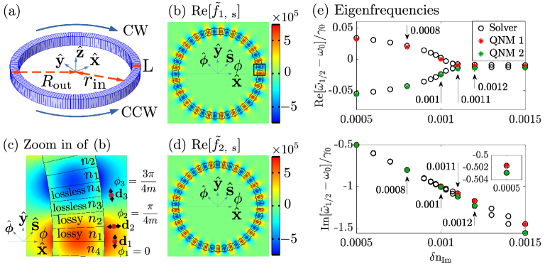
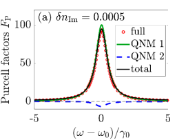
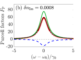
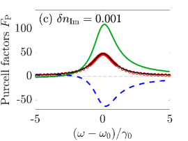
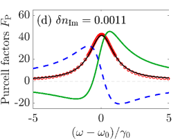
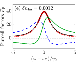
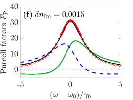
Figure 1: (a) 3D Schematic of a refractive-index-modulated ring resonator, though in our calculations we use a 2D model, partly because of large memory requirements for the resonators. The two blue arrows label the direction of CW and CCW of the fields. Field distribution ${\rm Re}\big{[}\tilde{f}_{s}\big{]}$ (with units $m^{-1}$, s components) ($\tilde{\bf f}=\tilde{f}_{x}\hat{\bf x}+\tilde{f}_{y}\hat{\bf y}=\tilde{f}_{s}\hat{\bf s}+\tilde{f}_{\phi}\hat{\bm{\phi}}$) of (b) QNM 1 (${\rm Re}\big{[}\tilde{f}_{1,\leavevmode\nobreak\ s}\big{]}$) and (d) QNM 2 (${\rm Re}\big{[}\tilde{f}_{2,\leavevmode\nobreak\ s}\big{]}$) for ring structures with $\delta n_{\rm Re}=\delta n_{\rm Im}=0.001$. (c) Zoom in of the black square in (b). (e) Eigenfrequencies from QNMs ($\tilde{\omega}_{1/2}=\omega_{1/2}-i\gamma_{1/2}$, red and green stars) and approximate COMSOL solver (black circles) for the ring resonator as a function of $\delta n_{\rm Im}$ when keeping $\delta n_{\rm Re}=0.001$. The insert in the bottom figure shows the zoom in region close to $\delta n_{\rm Im}=0.0005$. One will find that there are two efficient QNMs even when $\delta n_{\rm Re}=\delta n_{\rm Im}=0.001$. With the increase of $\delta n_{\rm Im}$, the decay rates of these QNMs increase. Specifically, later we will focus on six cases, including $\delta n_{\rm Im}=0.0005,0.0015$ and four more cases that the arrows points to.

Figure 2: Purcell factors from QNMs (Eq. (4)) and full numerical dipole method (Eq. (12)) for six cases investigated with the analytical two QNM expansion (separate contributions from QNM 1 and QNM 2, and the total contribution), including (a) $\delta n_{\rm Im}=0.0005$, (b) $\delta n_{\rm Im}=0.0008$, (c) $\delta n_{\rm Im}=0.001$, (d) $\delta n_{\rm Im}=0.0011$, (e) $\delta n_{\rm Im}=0.0012$, and (f) $\delta n_{\rm Im}=0.0015$, while keeping $\delta n_{\rm Re}=0.001$. The Purcell factors are for a LP $\hat{\bm{\phi}}$ dipole at $\phi=0$ (i.e., a LP $\hat{\bf y}$ dipole at $\phi=0$) and $10\leavevmode\nobreak\$nm away from the outer ring surface. $\omega_{0}$ and $\gamma_{0}$ are the real part and the opposite imaginary part of the pole eigenfrequency for QNM 1 with $\delta n_{\rm Im}=0.001$.

For numerical calculations, we consider a microring resonator similar to those in Refs. Chen et al., 2020; Martin-Cano et al., 2019, with a outer radius of $R_{\rm out}=1271\leavevmode\nobreak\$nm and a inner radius of $r_{\rm in}=1109$ nm (width of $L=R_{\rm out}-r_{\rm in}=162$ nm) (cf. Fig. 2(a)). The two blue arrows in Fig. 2(a) show the direction of CW and CCW fields. In our calculations, we investigate a 2D ring resonator and couple it with an in-plane LP dipole. This geometry yields a TE-like mode.

As shown in Fig. 2(c), the refractive index of the ring is modulated periodically (along the CCW direction), which has the following form Chen et al. (2020); Feng et al. (2014); Miao et al. (2016):

$$\begin{split}n_{1}&=n_{0}+\delta n_{\rm Re}+i\delta n_{\rm Im},\leavevmode\nobreak\ \big{[}l\pi/m<\phi<(l+1/4)\pi/m\big{]},\\ n_{2}&=n_{0}+i\delta n_{\rm Im},\leavevmode\nobreak\ \big{[}(l+1/4)\pi/m<\phi<(l+1/2)\pi/m\big{]},\\ n_{3}&=n_{0},\leavevmode\nobreak\ \big{[}(l+1/2)\pi/m<\phi<(l+3/4)\pi/m\big{]},\\ n_{4}&=n_{0}+\delta n_{\rm Re},\leavevmode\nobreak\ \big{[}(l+3/4)\pi/m<\phi<(l+1)\pi/m\big{]},\end{split}$$ (14)

where $l=0,1,2,\dots,2m-1$, and $m$ is the azimuthal mode number. There are $2m$ periods and $8m$ sections in total. Notably, such modulation only works for the mode with the specific azimuthal mode number $m$ (radial mode number is usually set as $q=1$, but the mode with $q=2$ etc. also has similar trends as $q=1$). In other words, one could design the modulation for the particular mode of interest. Here, we choose a TE mode with $q=1$, and $m=21$, whose resonance is around $752$ nm (visible spectrum). In the following, we will keep $n_{0}=3.0$ and $\delta n_{\rm Re}=0.001$, while $\delta n_{\rm Im}$ is changed in the range of $0.0005\sim 0.0015$ (positive, lossy materials; the case with gain will also be investigated in Sec. VI).

Using an efficient dipole-excitation QNM technique Bai et al. (2013), we employ a LP dipole, $\hat{\bm{\phi}}$, placed at $\phi=\phi_{1}=0$ (which is also a linear $\hat{\bf y}$ dipole at $\phi=0$) and $10\leavevmode\nobreak\$nm away from the ring surface (the bottom dipole $\mathbf{d}_{1}=d_{0}\hat{\bm{\phi}}=d_{0}\hat{\bf y}$ in Fig. 2(c), schematically showing its position and polarization). Two QNMs (which we label as QNM 1 and QNM 2) are found in the frequency regime of interest, whose eigenfrequencies ($\tilde{\omega}_{1}=\omega_{1}-i\gamma_{1}$ and $\tilde{\omega}_{2}=\omega_{2}-i\gamma_{2}$) are shown in Fig. 2(e) (red and green stars). We also investigate the eigenfrequecies from the approximate COMSOL direct eigenfrequency solver (black circles), which are generally highly accurate for high $Q$ resonators though it’s not a robust nonlinear eigenmode solver. The results agree well with those obtained from the dipole-excited QNM technique (since mainly we are dealing with high $Q$ resonators, around $2100$ to $6600$ for various modulated index cases). Specifically, the eigenfrequency of QNM 1 for $\delta n_{\rm Im}=0.001$ is $\omega_{0}-i\gamma_{0}\approx 2.50543552\times 10^{15}-i3.768337\times 10^{11}$ (${\rm rad/s}$), i.e., $\omega_{0}$ and $\gamma_{0}$ are defined as the real part and the opposite imaginary part of this pole eigenfrequency.

The QNM field distributions ${\rm Re}\big{[}\tilde{f}_{s}\big{]}$ (s components), with $\tilde{\bf f}=\tilde{f}_{x}\hat{\bf x}+\tilde{f}_{y}\hat{\bf y}=\tilde{f}_{s}\hat{\bf s}+\tilde{f}_{\phi}\hat{\bm{\phi}}$, of QNM 1 and QNM 2 for the ring structures, with $\delta n_{\rm Re}=\delta n_{\rm Im}=0.001$, are shown in Figs. 2(b) and (d). For clarity, the black square area in Fig. 2(b) is enlarged and shown in Fig. 2(c), where the detailed periodic refractive index is displayed. In addition to the general ($\hat{\bf x},\hat{\bf y}$) basis, we also utilize a polar ($\hat{\bf s},\hat{\bm{\phi}}$) basis. The corresponding unit vectors are related from $\hat{\bf s}=\hat{\bf x}\cos{\phi}+\hat{\bf y}\sin{\phi}$ and $\hat{\bm{\phi}}=-\hat{\bf x}\sin(\phi)+\hat{\bf y}\cos{\phi}$ (the positive direction of polar angle $\phi$ is along CCW direction).

As mentioned before, with the dipole QNM technique, we use a LP $\hat{\bm{\phi}}$ dipole at $\phi=0$ (the bottom one $\mathbf{d}_{1}$ in Fig. 2(c)). Once we obtain the QNMs, then we can easily couple them to any in-plane LP dipoles with any polarization using a general Green function theory described in Sec. II. We schematically show three example dipoles in Fig. 2(c), where one ($\mathbf{d}_{1}$) is a LP $\hat{\bm{\phi}}$ dipole at $\phi=\phi_{1}=0$ (i.e., $\hat{\bf y}$ dipole at $\phi=0$), one ($\mathbf{d}_{2}$) is a LP $\hat{\bf s}$ dipole at $\phi=\phi_{2}=\pi/4m$, and the left one ($\mathbf{d}_{3}$) is a LP $\hat{\bm{\phi}}$ dipole at $\phi=\phi_{2}=3\pi/4m$. For these dipole positions, we can model the emitted radiation analytically using the QNMs, and also from a direct solution of Maxwell’s equations. To verify the accuracy of our QNM predictions for dipole emitted radiation, we will carry out both approaches below. In addition, we will show the essential role of the QNM phase, and point out the clear failure of using a NM expansion for the Green function response.

IV Purcell factors versus frequency for different dipole locations

To confirm the accuracy of our two QNM description for the index-modulated ring resonators, we next calculate the Purcell factors analytically from the QNM properties (Eq. (4)) for a $\hat{\bm{\phi}}$ dipole at $\phi=0$ (equal to $\hat{\bf y}$ at $\phi=0$, $\mathbf{d}_{1}$ in Fig. 2 (c)), and compare them with the full numerical dipole method (Eq. (12)). For all configurations investigated, an excellent agreement is shown as a function of frequency as demonstrated in Fig. 2, where the results for six cases with the analytical two QNM expansion are studied, including $\delta n_{\rm Im}=0.0005,0.0008,0.001,0.0011,0.0012,0.0015$ while keeping $\delta n_{\rm Re}=0.001$. Their eigenfrequencies are marked in Fig. 2(e). Although there are no material gain regions in these resonators, we also note the appearance of modal negative Purcell factors. This level of agreement is unusual in the sense that the eigenmodes in Ref. Chen et al. (2020) were reported to be completely decoupled, which was used to argue a chiral emission, an effect that is not expected nor obtained for a regular ring resonator. We will connect to the power flow emission below, and show that it is also well explained in terms of the underlying QNMs.

V Chiral power flow from linearly polarized dipoles

To directly connect with the experimentally measured chirality in Ref. Chen et al., 2020 from LP dipole emitters, here we show chiral power flow using only the QNM propagators in a similar microring with refractive index modulation. We can easily obtain the power flow by computing the scattered fields and the Poynting vector from QNMs and the QNM propagator, and thus the calculations are basically instantaneous (see Eq. (7)).

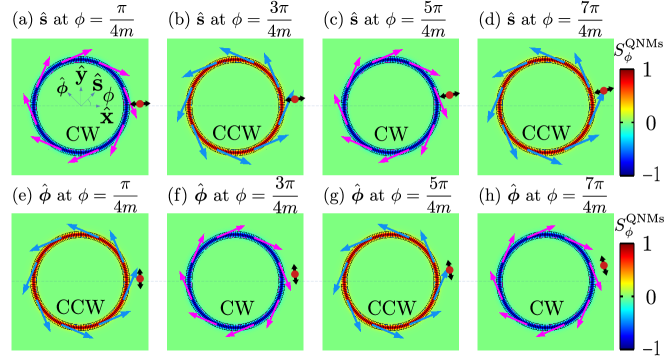
Figure 3: QNM calculations of power flow for various dipoles. We show the QNM Poynting vector ($\mathbf{S}^{\rm Poyn}_{\rm QNMs}=S_{x}^{\rm QNMs}\hat{\bf x}+S_{y}^{\rm QNMs}\hat{\bf{y}}=S_{s}^{\rm QNMs}\hat{\bf s}+S_{\phi}^{\rm QNMs}\hat{\bm{\phi}}$) using Eq. (7), for (a,b,c,d) $\hat{\bf s}$ and (e,f,g,h) $\hat{\bm{\phi}}$ dipoles at $\phi=\pi/4m$, $\phi=3\pi/4m$, $\phi=5\pi/4m$, and $\phi=7\pi/4m$ with $\delta n_{\rm Re}=\delta n_{\rm Im}=0.001$ (the radial distance between the dipole and the ring surface is $10\leavevmode\nobreak\$nm). The red dot with double black arrows schematically describes the position and polarization of the LP dipoles. The Poynting vectors are labelled with magenta (for CW direction) and blue (for CCW direction) arrows. The distributions show the projection $S^{\rm QNMs}_{\phi}$ along $\hat{\bm{\phi}}$. These power flows are calculated at an example real frequency of $\omega=2.50543\times 10^{15}$ (${\rm rad/s}$) (close to QNM resonance). In the ring region, one will find $S^{\rm QNMs}_{\phi}<0$ (it is shown in blue for the entire ring) for CW propagation and $S^{\rm QNMs}_{\phi}>0$ (red distribution in the entire ring) for CCW propagation.

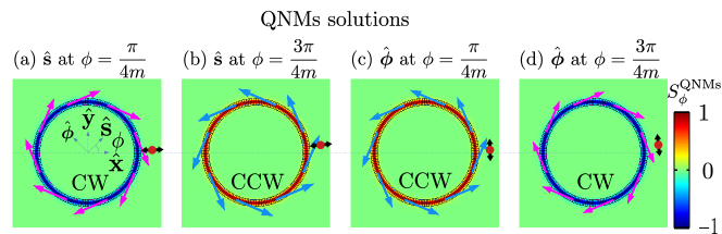
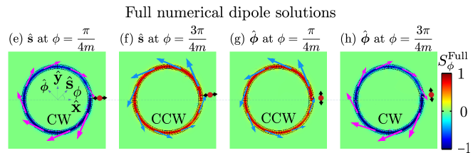
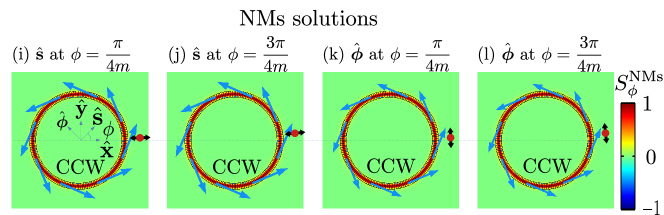
Figure 4: Power flow from (a-d) QNMs solutions (Eq. (7)), (e-h) full numerical dipole solutions (Eq. (13)) and (i-l) NMs solutions (Eq. (11)) for $\hat{\bf s}$ or $\hat{\bm{\phi}}$ at $\phi=\pi/4m$ or $\phi=3\pi/4m$. QNMs solutions recover the full numerical dipole results perfectly while the NM solutions fail in general (always CCW).

In this section, we focus on the case with $\delta n_{\rm Re}=\delta n_{\rm Im}=0.001$, which is closest to the EP as seen from Fig. 2(e) and Fig. 2(c). Figures 3(a-h) shows the chiral power flow (Eq. (7)) from our QNM model, for $\hat{\bf s}$ and $\hat{\bm{\phi}}$ dipole at several specific positions, including $\phi=\pi/4m$ (center of two lossy sections, see Fig. 2(c)), $\phi=3\pi/4m$ (center of two lossless sections), $\phi=5\pi/4m$ (center of two lossy sections), and $\phi=7\pi/4m$ (center of two lossless sections) (the radial distance between the dipole and the ring surface is $10\leavevmode\nobreak\$nm). The red dot with double black arrows in Fig. 3 schematically shows the position and polarization of these LP dipoles (though this is not to scale). Also note that these power flows presented in Fig. 3 are calculated at an examplary real frequency $\omega=2.50543\times 10^{15}$ (${\rm rad/s}$) (close to QNM resonance), and we stress that the chirality will remain the same in a range around $\omega_{0}\pm 1.5\gamma_{0}$.

The first thing to observe, is that when a LP $\hat{\bf s}$-dipole is placed at $\phi=\pi/4m$ (Fig. 3 (a)), the net power flow ($\mathbf{S}_{\rm QNMs}^{\rm Poyn}$, Eq. (7)), goes along the CW direction (indicated by the magenta arrows). The distribution shown is the projection $S_{\phi}^{\rm QNMs}$ along $\hat{\bm{\phi}}$. One will find that $S_{\phi}^{\rm QNMs}<0$ in the ring region, which further confirms that the net energy flow goes along the CW direction. This also supports the experimental findings in Ref. Chen et al., 2020, where they measured CW radiation when putting a LP dipole at $\phi=\pi/4l$ (center of lossy region) (azimuthal mode number $l=1$ in their considered structure, and we are using azimuthal mode number $m=21$ for a similar ring structure). However, our interpretation is drastically different. Instead of arguing with the help of a decoupling from the eigenmodes and coupling to a missing dimension, we find that our net chiral power flows are fully explained from the underlying QNMs, which are the correct natural eigenmodes of such resonators.

In addition, the azimuthal period of such phenomenon is $\pi/m$, i.e., when a LP $\hat{\bf s}$ dipole is located at $\phi=\frac{\pi}{4m}+p\frac{\pi}{m}$ (center of the two lossy regions), where $p=0,1,2,...2m-1$, the net power flow will go along the CW direction, such as at $\phi=5\pi/4m$ shown in Fig. 3 (c).

Moreover, we also find that such unusual properties are not limited to $\hat{\bf s}$ dipoles at $\phi=\frac{\pi}{4m}+p\frac{\pi}{m}$ ($p=0,1,2,...2m-1$). As shown in Fig. 3 (b,d), when a LP $\hat{\bf s}$ dipole is placed at $\phi=\frac{3\pi}{4m}+p\frac{\pi}{m}$ (center of the two lossless sections, where $p=0,1,2,...2m-1$), the net power flow is along the CCW direction, confirmed with both Poynting vectors $\mathbf{S}_{\rm QNMs}^{\rm Poyn}$ (Eq. (7)) (blue arrows) and projection $S_{\phi}^{\rm QNMs}>0$.

Furthermore, we found that such special chiral radiation are not only found with $\hat{\bf s}$ dipoles but also with LP $\hat{\bm{\phi}}$ dipole. As shown in Fig. 3 (e-h), when a LP $\hat{\bm{\phi}}$ dipole is placed at $\phi=\frac{\pi}{4m}+p\frac{\pi}{m}$ ($\phi=\frac{3\pi}{4m}+p\frac{\pi}{m}$, $p=0,1,2,...2m-1$), the net power flow will go along the CCW (CW) direction, again confirmed with Poynting vectors $\mathbf{S}_{\rm QNMs}^{\rm Poyn}$ with blue arrows (magenta arrows) and projection $S_{\phi}^{\rm QNMs}>0$ ($<0$).

To further justify that our QNM picture is both correct and rigorously accurate for describing this chiral emission, we have confirmed these unusual properties with full numerical dipole calculations as well as NM solutions. For a comprehensive comparison, we will focus on four cases, i.e., $\hat{\bf s}$ or $\hat{\bm{\phi}}$ dipoles placed at $\phi=\pi/4m$ or $\phi=3\pi/4m$, and all other special cases could be obtained automatically due to the periodic modulated index. For convenience, we show the QNM solutions given in Fig. 3 (a-b) and (e-f) again in Fig. 4 (a-d). The corresponding full numerical dipole solutions (Eq. (13)) are shown in Fig. 4 (e-h), and one will find excellent agreement between QNM solutions and full numerical dipole solutions.

It is also insightful to compare with a NM solution, to assess the role of the QNM phase. In contrast to the QNM approach, the NM model (Eq. (11)) fails to capture the crucial effect of the change of power flow direction. Indeed, as shown in Fig. 4 (i-l), the flow direction always stays in CCW direction no matter where the dipole is placed and how it it polarized. To investigate this in more detail, we inspect the analytical structure of the power flow formulas. We recognize, that the crucial difference appears in the off-diagonal elements of the Poynting vector. To see this more clearly, we rewrite the Poynting vectors as $\mathbf{S}^{\rm Poyn}_{\rm NMs}=\mathbf{S}^{\rm Poyn}_{\rm ref}+\sin(\theta_{1}-\theta_{2})\mathbf{S}^{\rm Poyn}_{\rm diff}$ and $\mathbf{S}^{\rm Poyn}_{\rm QNMs}=\mathbf{S}^{\rm Poyn}_{\rm ref}-\sin(\theta_{1}-\theta_{2})\mathbf{S}^{\rm Poyn}_{\rm diff}$, where $\theta_{1},\theta_{2}$ are the complex phases of the dipole-projected QNM eigenfunctions 1,2 ($\tilde{\mathbf{f}}_{1/2}(\mathbf{r}_{d})\cdot\mathbf{n}_{\rm d}=\big{|}\tilde{\mathbf{f}}_{1/2}(\mathbf{r}_{d})\cdot\mathbf{n}_{\rm d}\big{|}e^{i\theta_{1/2}}=\big{|}\tilde{f}_{1/2,\rm d}(\mathbf{r}_{\rm d})\big{|}e^{i\theta_{1/2}}$) and

$$\mathbf{S}^{\rm Poyn}_{\rm diff} (\mathbf{r},\omega)$$

$$= \big{|}\tilde{f}_{1,\rm d}(\mathbf{r}_{\rm d})\big{|}\big{|}\tilde{f}_{2,\rm d}(\mathbf{r}_{\rm d})\big{|}{\rm Re}\big{[}A_{1}(\omega)A_{2}^{*}(\omega)\tilde{\mathbf{s}}_{12}(\mathbf{r},\omega)\big{]}$$

$$-\big{|}\tilde{f}_{1,\rm d}(\mathbf{r}_{\rm d})\big{|}\big{|}\tilde{f}_{2,\rm d}(\mathbf{r}_{\rm d})\big{|}{\rm Re}\big{[}A_{2}(\omega)A_{1}^{*}(\omega)\tilde{\mathbf{s}}_{21}(\mathbf{r},\omega)\big{]},$$ (15)

with $\tilde{\mathbf{s}}_{12}(\mathbf{r},\omega)=\tilde{\mathbf{f}}_{1}(\mathbf{r})\times\big{[}\bm{\nabla}\times\tilde{\mathbf{f}}_{2}^{*}(\mathbf{r})\big{]}/(2\mu_{0}\omega)$ and $\tilde{\mathbf{s}}_{21}(\mathbf{r},\omega)=\tilde{\mathbf{f}}_{2}(\mathbf{r})\times\big{[}\bm{\nabla}\times\tilde{\mathbf{f}}_{1}^{*}(\mathbf{r})\big{]}/(2\mu_{0}\omega)$.

The sign difference between the QNM and NM model is induced by use of the unconjugated and conjugated form, respectively, and depends on the difference of the QNM phases, which are highly position-dependent. In that sense, even if we take full account of the QNM eigenfrequency and eigenfunctions for the NM model, it does not recover the crucial change of the power flow direction, and applying the usual NM assumptions would lead to even more differences.

VI Discussion on frequency dependent chiral flow and chiral flow with gain media

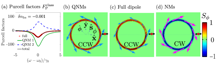
Figure 5: Ring resonators with gain. (a) Classical Purcell factors (Eq. (4), here we refer it as $F_{\rm P}^{\rm class}$) from the QNMs. The power flow of a LP $\hat{\bf s}$ dipole at $\phi=\pi/4m$ from (b) QNMs solutions, (c) full numerical dipole solutions and (d) NMs solutions for ring resonator with gain ($\delta n_{\rm Im}=-0.001$, $\delta n_{\rm Re}=0.001$).

Apart from above discussed position and polarization-dependent chiral radiation, we also observe, that the chirality is sensitive to a change in frequency at special locations. For example, for $\hat{\bf s}$ dipoles at $\phi=p\frac{\pi}{m}$ ($p=0,1,2,...2m-1$) and $\phi=\frac{2\pi}{4m}+p\frac{\pi}{m}$ (cf. Fig. 2), respectively, the power flow direction will change from CCW to CW and from CW to CCW, when tuning $\omega$ through the resonance, i.e., at resonance, there is no net CW or CCW power flow. Similar behaviour can also be found for $\hat{\bm{\phi}}$ dipoles, where the power flow direction will change from CW (CCW) to CCW (CW) at $\phi=p\frac{\pi}{m}$ ($\phi=\frac{2\pi}{4m}+p\frac{\pi}{m}$, $p=0,1,2,...2m-1$). This gives one an external control method to change the directionality by simply changing the frequency.

In the current design, there is no gain materials involved. However, in general, as also mentioned in Ref. Chen et al., 2020, one could also add gain material into the investigated ring resonator structure. As an example, the results for the case with $\delta n_{\rm Im}=-0.001$ ($\delta n_{\rm Re}=0.001$) are shown in Fig. 5. Two effective QNMs are found, whose total contribution to Purcell factors are net-negative (see Fig. 5 (a)), which are unphysical as recently demonstrated in Ref. Franke et al., 2021, i.e., when the gain is present, the classical formula of the Purcell factor (Eq. (4), here we refer it as $F_{\rm P}^{\rm class}$), and the traditional Fermi’s golden rule for spontaneous emission decay do not work. However, the negative LDOS is correct and physical, and in agreement with the classical full numerical dipole result (red circles). To obtain the correct Purcell factor in amplifying dielectric media, a quantum mechanical fix is required as shown in Ref. Franke et al., 2021, which results in (for a dipole with real dipole moment $\mathbf{d}$)

$$F_{\rm P}^{\rm QM}({\bf r}_{\rm d})=F_{\rm P}^{\rm class}({\bf r}_{\rm d})+\frac{2\mathbf{d}\cdot\mathbf{K}^{\rm gain}(\mathbf{r}_{\rm d},\mathbf{r}_{\rm d},\omega)\cdot\mathbf{d}}{\hbar\epsilon_{0}\Gamma_{0}},$$ (16)

where the second term is a positive gain-induced correction term, which will bring the total values to be correct net-positive $F_{\rm P}^{\rm QM}$. In more detail, the general form of $\mathbf{K}^{\rm gain}(\mathbf{r}_{\rm d},\mathbf{r}_{\rm d},\omega)$ could be written as Franke et al. (2021)

$$\begin{split}\mathbf{K}^{\rm gain}(\mathbf{r}_{\rm d},\mathbf{r}_{\rm d},\omega)&\\ =\int_{A_{\rm gain}}d\mathbf{s}&\big{|}{\rm Im}[\epsilon_{\rm gain}(\mathbf{s})]\big{|}\mathbf{G}(\mathbf{r}_{\rm d},\mathbf{s},\omega)\cdot\mathbf{G}^{*}(\mathbf{s},\mathbf{r}_{\rm d},\omega),\end{split}$$ (17)

which are closely related with the Green function (Eq. (3)), i.e., the two underlying QNMs, and the permittivity $\epsilon_{\rm gain}=n_{\rm gain}^{2}$ within the gain region $A_{\rm gain}$. Here we do not compute this quantum mechanical fix to the SE rate, but further details are discussed in Refs. Franke et al., 2021; Ren et al., 2021a.

In addition, the corresponding power flows from a linear dipole $\hat{\bf s}$ at $\phi=\pi/4m$ are shown in Fig. 5 (b-d). Again, the QNM solution shows excellent agreement (both along CCW) with full numerical dipole solution, while the NM solution doesn’t because the phases are ignored. Moreover, compared with the ring with lossy materials (see Fig. 3 (a), or Fig. 4(a) and (e); along CW), the power flow with gain materials reverses to the opposite direction (Fig. 5 (b-c); along CCW), which is true for all the special cases such as those shown in Fig. 3, though here (Fig. 5) we only show one of the examples. The reversed chiral power flow are closely related with the properties of the two underling QNMs with gain media, which are approximately differing $\pi$ on QNMs phases for $\tilde{\mathbf{f}}_{1/2}$, compared with those two QNMs with lossy media. In addition, the imaginary parts of the corresponding QNM complex eigenfrequencies $\tilde{\omega}_{1/2}$ also change from negative to positive (gain mode). Taking these changes into account, the analytical power flow expression Eq. (7) could exactly predict the reversed chirality.

Also note that such chirality behavior is not found in regular ring resonators (without a refractive modulation) for LP $\hat{\bf s}$ and $\hat{\bm{\phi}}$ dipoles, i.e., no net power flow is obtained. However, by using a circular-polarized dipole close to or inside the general ring resonator, chirality will exist, as shown in Ref. Martin-Cano et al., 2019, where positional dependent chirality for right- or left-handed circular dipoles are demonstrated. This is also similar to how one excites unidirectional propagation in photonic crystal waveguides Young et al. (2015); Söllner et al. (2015). However, in all these cases, local symmetry breaking is possible by using a circularly polarized dipole.

VII Conclusions

We have investigated EP-like resonances formed from index-modulated ring resonators, where unusual chiral radiation from LP dipoles was recently observed Chen et al. (2020). We showed that the full numerical dipole Purcell factor response is quantitatively well explained in terms of the two dominating QNMs of this resonator, which could be negative in part of the frequency range, but the total contribution from two QNMs is always net-positive (for a lossy material system). In particular, when a LP $\hat{\bf s}$ dipole is located at $\phi=\pi/4m$, the analytical Poynting vectors obtained from the QNM propagator goes along the CW direction, which supports the experimental findings in Ref. Chen et al., 2020 for similar ring resonators.

Notably, our explanation is in contrast with the view that the emitter does not couple to the eigenmodes of the system. This is mainly because the QNMs are the correct eigenmodes and the perfect EP does not exists for our simulations, and the symmetry is naturally broken to allow chiral emission. In addition, we also showed how such chirality is not limited to $\hat{\bf s}$ dipoles at $\phi=\frac{\pi}{4m}+p\frac{\pi}{m}$ ($p=0,1,2,...2m-1$), and we also demonstrated the opposite chirality for $\hat{\bf s}$ dipoles at $\phi=\frac{3\pi}{4m}+p\frac{\pi}{m}$ ($p=0,1,2,...2m-1$). There is also similar chirality for linearly $\hat{\bm{\phi}}$ dipoles at these positions. All of these net power flows can be well explained and interpreted from the two underling QNMs and the corresponding Green function, where the QNM phases play a decisive and fundamental role on the light emission, without having to invoke any unusual interpretation such as a missing dimension (Jordan vector). In comparison, we also showed how a NM model fails to capture the correct power flow since it takes no account of the essential phases. Moreover, frequency dependent chiral radiation was also investigated, which adds another degree of freedom to control the chirality in addition to the position and orientation of the emitter.

Lastly, we showed that when the lossy materials are replaced by gain materials in the index modulation, again two working classical QNMs are found, whose total contributions on the classical Purcell factors can be net-negative; this is a general failure of the classical theory, but can be fixed to ensure a net-positive value through a quantum mechanical correction term Franke et al. (2021). In addition, the corresponding power flow direction will reverse compared to those with lossy materials.

References

- Vahala (2013) K. J. Vahala, “Optical microcavities,” Nature 424, 839–846 (2013).
- Maier (2007) Stefan Alexander Maier, Plasmonics: fundamentals and applications (Springer Science & Business Media, 2007).
- Chang et al. (2006) D. E. Chang, A. S. Sørensen, P. R. Hemmer, and M. D. Lukin, “Quantum optics with surface plasmons,” Physical Review Letters 97, 053002 (2006).
- Benson (2011) Oliver Benson, “Assembly of hybrid photonic architectures from nanophotonic constituents,” Nature 480, 193–199 (2011).
- Jacob and Shalaev (2011) Zubin Jacob and Vladimir M. Shalaev, “Plasmonics goes quantum,” Science 334, 463–464 (2011).
- Van Vlack et al. (2012) C. Van Vlack, Philip Trøst Kristensen, and S. Hughes, “Spontaneous emission spectra and quantum light-matter interactions from a strongly coupled quantum dot metal-nanoparticle system,” Phys. Rev. B 85, 075303 (2012).
- Tame et al. (2013) M. S. Tame, K. R. McEnery, Ş. K. Özdemir, J. Lee, S. A. Maier, and M. S. Kim, “Quantum plasmonics,” Nature Physics 9, 329–340 (2013).
- Lian et al. (2015) Hang Lian, Ying Gu, Juanjuan Ren, Fan Zhang, Luojia Wang, and Qihuang Gong, “Efficient single photon emission and collection based on excitation of gap surface plasmons,” Physical Review Letters 114, 193002 (2015).
- Chikkaraddy et al. (2016) Rohit Chikkaraddy, Bart de Nijs, Felix Benz, Steven J. Barrow, Oren A. Scherman, Edina Rosta, Angela Demetriadou, Peter Fox, Ortwin Hess, and Jeremy J. Baumberg, “Single-molecule strong coupling at room temperature in plasmonic nanocavities,” Nature 535, 127–130 (2016).
- Ren et al. (2017) Juanjuan Ren, Ying Gu, Dongxing Zhao, Fan Zhang, Tiancai Zhang, and Qihuang Gong, “Evanescent-vacuum-enhanced photon-exciton coupling and fluorescence collection,” Physical Review Letters 118, 073604 (2017).
- Tong et al. (2003) Limin Tong, Rafael R. Gattass, Jonathan B. Ashcom, Sailing He, Jingyi Lou, Mengyan Shen, Iva Maxwell, and Eric Mazur, “Subwavelength-diameter silica wires for low-loss optical wave guiding,” Nature 426, 816–819 (2003).
- Tong et al. (2004) Limin Tong, Jingyi Lou, and Eric Mazur, “Single-mode guiding properties of subwavelength-diameter silica and silicon wire waveguides,” Optics Express 12, 1025 (2004).
- Akimov et al. (2007) A. V. Akimov, A. Mukherjee, C. L. Yu, D. E. Chang, A. S. Zibrov, P. R. Hemmer, H. Park, and M. D. Lukin, “Generation of single optical plasmons in metallic nanowires coupled to quantum dots,” Nature 450, 402–406 (2007).
- Yalla et al. (2012) Ramachandrarao Yalla, Fam Le Kien, M. Morinaga, and K. Hakuta, “Efficient channeling of fluorescence photons from single quantum dots into guided modes of optical nanofiber,” Physical Review Letters 109, 063602 (2012).
- Yalla et al. (2014) Ramachandrarao Yalla, Mark Sadgrove, Kali P. Nayak, and Kohzo Hakuta, “Cavity quantum electrodynamics on a nanofiber using a composite photonic crystal cavity,” Physical Review Letters 113, 143601 (2014).
- Kato and Aoki (2015) Shinya Kato and Takao Aoki, “Strong coupling between a trapped single atom and an all-fiber cavity,” Physical Review Letters 115, 093603 (2015).
- Akahane et al. (2003) Yoshihiro Akahane, Takashi Asano, Bong-Shik Song, and Susumu Noda, “High-q photonic nanocavity in a two-dimensional photonic crystal,” Nature 425, 944–947 (2003).
- Yoshie et al. (2004) T. Yoshie, A. Scherer, J. Hendrickson, G. Khitrova, H. M. Gibbs, G. Rupper, C. Ell, O. B. Shchekin, and D. G. Deppe, “Vacuum rabi splitting with a single quantum dot in a photonic crystal nanocavity,” Nature 432, 200–203 (2004).
- Goban et al. (2015) A. Goban, C.-L. Hung, J.D. Hood, S.-P. Yu, J.A. Muniz, O. Painter, and H.J. Kimble, “Superradiance for atoms trapped along a photonic crystal waveguide,” Physical Review Letters 115, 063601 (2015).
- Söllner et al. (2015) Immo Söllner, Sahand Mahmoodian, Sofie Lindskov Hansen, Leonardo Midolo, Alisa Javadi, Gabija Kiršanskė, Tommaso Pregnolato, Haitham El-Ella, Eun Hye Lee, Jin Dong Song, Søren Stobbe, and Peter Lodahl, “Deterministic photon–emitter coupling in chiral photonic circuits,” Nature Nanotechnology 10, 775–778 (2015).
- le Feber et al. (2015) B. le Feber, N. Rotenberg, and L. Kuipers, “Nanophotonic control of circular dipole emission,” Nature Communications 6, 6695 (2015).
- Lodahl et al. (2017) Peter Lodahl, Sahand Mahmoodian, Søren Stobbe, Arno Rauschenbeutel, Philipp Schneeweiss, Jürgen Volz, Hannes Pichler, and Peter Zoller, “Chiral quantum optics,” Nature 541, 473–480 (2017).
- Zhang et al. (2019) Fan Zhang, Juanjuan Ren, Lingxiao Shan, Xueke Duan, Yan Li, Tiancai Zhang, Qihuang Gong, and Ying Gu, “Chiral cavity quantum electrodynamics with coupled nanophotonic structures,” Physical Review A 100, 053841 (2019).
- Young et al. (2015) A. B. Young, A. C. T. Thijssen, D. M. Beggs, P. Androvitsaneas, L. Kuipers, J. G. Rarity, S. Hughes, and R. Oulton, “Polarization engineering in photonic crystal waveguides for spin-photon entanglers,” Physical Review Letters 115, 153901 (2015).
- Jalas et al. (2013) Dirk Jalas, Alexander Petrov, Manfred Eich, Wolfgang Freude, Shanhui Fan, Zongfu Yu, Roel Baets, Milos̆ Popović, Andrea Melloni, John D. Joannopoulos, Mathias Vanwolleghem, Christopher R. Doerr, and Hagen Renner, “What is - and what is not - an optical isolator,” Nature Photonics 7, 579–582 (2013).
- Sayrin et al. (2015) Clément Sayrin, Christian Junge, Rudolf Mitsch, Bernhard Albrecht, Danny O’Shea, Philipp Schneeweiss, Jürgen Volz, and Arno Rauschenbeutel, “Nanophotonic optical isolator controlled by the internal state of cold atoms,” Physical Review X 5, 041036 (2015).
- Kimble (2008) H. J. Kimble, “The quantum internet,” Nature 453, 1023–1030 (2008).
- Leung et al. (1994a) P. T. Leung, S. Y. Liu, and K. Young, “Completeness and orthogonality of quasinormal modes in leaky optical cavities,” Physical Review A 49, 3057–3067 (1994a).
- Mazzei et al. (2007) A. Mazzei, S. Götzinger, L. de S. Menezes, G. Zumofen, O. Benson, and V. Sandoghdar, “Controlled coupling of counterpropagating whispering-gallery modes by a single rayleigh scatterer: A classical problem in a quantum optical light,” Physical Review Letters 99, 173603 (2007).
- Teraoka and Arnold (2009) Iwao Teraoka and Stephen Arnold, “Resonance shifts of counterpropagating whispering-gallery modes: degenerate perturbation theory and application to resonator sensors with axial symmetry,” Journal of the Optical Society of America B 26, 1321 (2009).
- Righini et al. (2011) G. C. Righini, Y. Dumeige, P. Féron, M. Ferrari, G. Nunzi Conti, D. Ristic, and S. Soria, “Whispering gallery mode microresonators: Fundamentals and applications,” La Rivista del Nuovo Cimento 34, 435–488 (2011).
- Schunk et al. (2014) Gerhard Schunk, Josef U. Fürst, Michael Förtsch, Dmitry V. Strekalov, Ulrich Vogl, Florian Sedlmeir, Harald G. L. Schwefel, Gerd Leuchs, and Christoph Marquardt, “Identifying modes of large whispering-gallery mode resonators from the spectrum and emission pattern,” Optics Express 22, 30795 (2014).
- Cognée et al. (2019) Kévin G. Cognée, Hugo M. Doeleman, Philippe Lalanne, and A. F. Koenderink, “Cooperative interactions between nano-antennas in a high-Q cavity for unidirectional light sources,” Light: Science & Applications 8, 115 (2019).
- Martin-Cano et al. (2019) Diego Martin-Cano, Harald R. Haakh, and Nir Rotenberg, “Chiral emission into nanophotonic resonators,” ACS Photonics 6, 961–966 (2019).
- Peng et al. (2014a) Bo Peng, Şahin Kaya Özdemir, Fuchuan Lei, Faraz Monifi, Mariagiovanna Gianfreda, Gui Lu Long, Shanhui Fan, Franco Nori, Carl M. Bender, and Lan Yang, “Parity–time-symmetric whispering-gallery microcavities,” Nature Physics 10, 394–398 (2014a).
- Chang et al. (2014) Long Chang, Xiaoshun Jiang, Shiyue Hua, Chao Yang, Jianming Wen, Liang Jiang, Guanyu Li, Guanzhong Wang, and Min Xiao, “Parity-time symmetry and variable optical isolation in active-passive-coupled microresonators,” Nature Photon. 8, 524–529 (2014).
- Chen et al. (2018) Weijian Chen, Jing Zhang, Bo Peng, Şahin Kaya Özdemir, Xudong Fan, and Lan Yang, “Parity-time-symmetric whispering-gallery mode nanoparticle sensor [invited],” Photonics Research 6, A23–A30 (2018).
- Berry (2004) M.V. Berry, “Physics of nonhermitian degeneracies,” Czechoslovak Journal of Physics 54, 1039–1047 (2004).
- Heiss (2004) W D Heiss, “Exceptional points of non-hermitian operators,” J. Phys. A: Math. Gen. 37, 2455–2464 (2004).
- Heiss (2012) W D Heiss, “The physics of exceptional points,” J. Phys. A: Math. Theor. 45, 444016 (2012).
- Ding et al. (2016) Kun Ding, Guancong Ma, Meng Xiao, Z. Q. Zhang, and C. T. Chan, “Emergence, coalescence, and topological properties of multiple exceptional points and their experimental realization,” Phys. Rev. X 6, 021007 (2016).
- Miri and Alù (2019) Mohammad-Ali Miri and Andrea Alù, “Exceptional points in optics and photonics,” Science 363, eaar7709 (2019).
- Chen et al. (2019) Chong Chen, Liang Jin, and Ren-Bao Liu, “Sensitivity of parameter estimation near the exceptional point of a non-hermitian system,” New Journal of Physics 21, 083002 (2019).
- Jin et al. (2020) L. Jin, H. C. Wu, Bo-Bo Wei, and Z. Song, “Hybrid exceptional point created from type-III dirac point,” Physical Review B 101, 045130 (2020).
- Chen et al. (2020) Hua-Zhou Chen, Tuo Liu, Hong-Yi Luan, Rong-Juan Liu, Xing-Yuan Wang, Xue-Feng Zhu, Yuan-Bo Li, Zhong-Ming Gu, Shan-Jun Liang, He Gao, Ling Lu, Li Ge, Shuang Zhang, Jie Zhu, and Ren-Min Ma, “Revealing the missing dimension at an exceptional point,” Nature Physics 16, 571–578 (2020).
- Chen et al. (2017) Weijian Chen, Şahin Kaya Özdemir, Guangming Zhao, Jan Wiersig, and Lan Yang, “Exceptional points enhance sensing in an optical microcavity,” Nature 548, 192–196 (2017).
- Ren et al. (2021a) Juanjuan Ren, Sebastian Franke, and Stephen Hughes, “Quasinormal modes, local density of states, and classical purcell factors for coupled loss-gain resonators,” Physical Review X 11, 041020 (2021a).
- (48) Sebastian Franke, Juanjuan Ren, and Stephen Hughes, “Quantized quasinormal mode theory of coupled lossy and amplifying resonators,” arxiv:2109.14967 .
- Wiersig (2020) Jan Wiersig, “Review of exceptional point-based sensors,” Photonics Research 8, 1457 (2020).
- Peng et al. (2014b) B. Peng, Ş. K. Özdemir, S. Rotter, H. Yilmaz, M. Liertzer, F. Monifi, C. M. Bender, F. Nori, and L. Yang, “Loss-induced suppression and revival of lasing,” Science 346, 328–332 (2014b).
- Hodaei et al. (2014) H. Hodaei, M.-A. Miri, M. Heinrich, D. N. Christodoulides, and M. Khajavikhan, “Parity-time-symmetric microring lasers,” Science 346, 975–978 (2014).
- Hayenga et al. (2020) W. E. Hayenga, H. Garcia-Gracia, E. Sanchez Cristobal, M. Parto, H. Hodaei, P. LiKamWa, D. N. Christodoulides, and M. Khajavikhan, “Electrically pumped microring parity-time-symmetric lasers,” Proceedings of the IEEE 108, 827–836 (2020), conference Name: Proceedings of the IEEE.
- Peng et al. (2016) Bo Peng, Şahin Kaya Özdemir, Matthias Liertzer, Weijian Chen, Johannes Kramer, Huzeyfe Yılmaz, Jan Wiersig, Stefan Rotter, and Lan Yang, “Chiral modes and directional lasing at exceptional points,” Proceedings of the National Academy of Sciences 113, 6845–6850 (2016).
- Wiersig (2016) Jan Wiersig, “Sensors operating at exceptional points: General theory,” Physical Review A 93, 033809 (2016).
- Cai et al. (2012) Xinlun Cai, Jianwei Wang, Michael Strain, Benjamin Johnson-Morris, Jiangbo Zhu, Erman Engin, Ying-Lung Ho, Marc Sorel, Jeremy L. O’Brien, Mark Thompson, and Siyuan Yu, “Integrated compact optical vortex beam emitters,” Science 338, 363–366 (2012).
- Feng et al. (2014) L. Feng, Z. J. Wong, R.-M. Ma, Y. Wang, and X. Zhang, “Single-mode laser by parity-time symmetry breaking,” Science 346, 972–975 (2014).
- Miao et al. (2016) Pei Miao, Zhifeng Zhang, Jingbo Sun, Wiktor Walasik, Stefano Longhi, Natalia M. Litchinitser, and Liang Feng, “Orbital angular momentum microlaser,” Science 353, 464–467 (2016).
- Lai et al. (1990) H. M. Lai, P. T. Leung, K. Young, P. W. Barber, and S. C. Hill, “Time-independent perturbation for leaking electromagnetic modes in open systems with application to resonances in microdroplets,” Phys. Rev. A 41, 5187–5198 (1990).
- Leung et al. (1994b) P. T. Leung, S. Y. Liu, S. S. Tong, and K. Young, “Time-independent perturbation theory for quasinormal modes in leaky optical cavities,” Physical Review A 49, 3068–3073 (1994b).
- Leung and Pang (1996) P. T. Leung and K. M. Pang, “Completeness and time-independent perturbation of morphology-dependent resonances in dielectric spheres,” JOSAB 13, 805–817 (1996).
- Lee et al. (1999) K. M. Lee, P. T. Leung, and K. M. Pang, “Dyadic formulation of morphology-dependent resonances. i. completeness relation,” JOSAB 16, 1409–1417 (1999).
- Kristensen et al. (2012) P. T. Kristensen, C. Van Vlack, and S. Hughes, “Generalized effective mode volume for leaky optical cavities,” Optics Letters 37, 1649 (2012).
- Sauvan et al. (2013) C. Sauvan, J. P. Hugonin, I. S. Maksymov, and P. Lalanne, “Theory of the Spontaneous Optical Emission of Nanosize Photonic and Plasmon Resonators,” Physical Review Letters 110, 237401 (2013).
- Kristensen and Hughes (2014) Philip Trøst Kristensen and Stephen Hughes, “Modes and Mode Volumes of Leaky Optical Cavities and Plasmonic Nanoresonators,” ACS Photonics 1, 2–10 (2014).
- Ge and Hughes (2014) Rong-Chun Ge and S. Hughes, “Design of an efficient single photon source from a metallic nanorod dimer: a quasi-normal mode finite-difference time-domain approach,” Opt. Lett. 39, 4235 (2014).
- Zschiedrich et al. (2018) Lin Zschiedrich, Felix Binkowski, Niko Nikolay, Oliver Benson, Günter Kewes, and Sven Burger, “Riesz-projection-based theory of light-matter interaction in dispersive nanoresonators,” Phys. Rev. A 98, 043806 (2018).
- Alpeggiani et al. (2017) Filippo Alpeggiani, Nikhil Parappurath, Ewold Verhagen, and L. Kuipers, “Quasinormal-mode expansion of the scattering matrix,” Phys. Rev. X 7, 021035 (2017).
- Lalanne et al. (2018) Philippe Lalanne, Wei Yan, Kevin Vynck, Christophe Sauvan, and Jean-Paul Hugonin, “Light interaction with photonic and plasmonic resonances,” Laser & Photonics Reviews 12, 1700113 (2018).
- Kristensen et al. (2020) Philip Trøst Kristensen, Kathrin Herrmann, Francesco Intravaia, and Kurt Busch, “Modeling electromagnetic resonators using quasinormal modes,” Advances in Optics and Photonics 12, 612 (2020).
- Franke et al. (2021) Sebastian Franke, Juanjuan Ren, Marten Richter, Andreas Knorr, and Stephen Hughes, “Fermi’s golden rule for spontaneous emission in absorptive and amplifying media,” Physical Review Letters 127, 013602 (2021).
- Kristensen et al. (2015) Philip Trøst Kristensen, Rong-Chun Ge, and Stephen Hughes, “Normalization of quasinormal modes in leaky optical cavities and plasmonic resonators,” Phys. Rev. A 92, 053810 (2015).
- Ren et al. (2021b) Juanjuan Ren, Sebastian Franke, and Stephen Hughes, “Quasinormal modes, local density of states, and classical Purcell factors for coupled loss-gain resonators,” Phys. Rev. X 11, 041020 (2021b).
- Ge et al. (2014) Rong-Chun Ge, Philip Trøst Kristensen, Jeff F Young, and Stephen Hughes, “Quasinormal mode approach to modelling light-emission and propagation in nanoplasmonics,” New Journal of Physics 16, 113048 (2014).
- Anger et al. (2006) Pascal Anger, Palash Bharadwaj, and Lukas Novotny, “Enhancement and quenching of single-molecule fluorescence,” Phys. Rev. Lett. 96, 113002 (2006).
- (75) COMSOL Inc., “Comsol multiphysics v 5.6,” www.comsol.com.
- Franke et al. (2019) Sebastian Franke, Stephen Hughes, Mohsen Kamandar Dezfouli, Philip Trøst Kristensen, Kurt Busch, Andreas Knorr, and Marten Richter, “Quantization of quasinormal modes for open cavities and plasmonic cavity quantum electrodynamics,” Phys. Rev. Lett. 122, 213901 (2019).
- Franke et al. (2020) Sebastian Franke, Marten Richter, Juanjuan Ren, Andreas Knorr, and Stephen Hughes, “Quantized quasinormal-mode description of nonlinear cavity-QED effects from coupled resonators with a Fano-like resonance,” Phys. Rev. Research 2, 033456 (2020).
- Bai et al. (2013) Q. Bai, M. Perrin, C. Sauvan, J.-P. Hugonin, and P. Lalanne, “Efficient and intuitive method for the analysis of light scattering by a resonant nanostructure,” Optics Express 21, 27371–27382 (2013).