Scale up to infinity: the UWB Indoor Global Positioning System

Abstract

Determining assets position with high accuracy and scalability is one of the most investigated technology on the market. The accuracy provided by satellites-based positioning systems (i.e., GLONASS or Galileo) is not always sufficient when a decimeter-level accuracy is required or when there is the need of localising entities that operate inside indoor environments. Scalability is also a recurrent problem when dealing with indoor positioning systems. This paper presents an innovative UWB Indoor GPS-Like local positioning system able to tracks any number of assets without decreasing measurements update rate. To increase the system’s accuracy the mathematical model and the sources of uncertainties are investigated. Results highlight how the proposed implementation provides positioning information with an absolute maximum error below 20 cm. Scalability is also resolved thanks to DTDoA transmission mechanisms not requiring an active role from the asset to be tracked.

I Introduction

As an accurate positioning system is the mainstay of most mobile robot applications [1], researchers have proposed to implement different LPS to provide an indoor localisation infrastructure. As described in [2] positioning systems can be classified into two macro classes: 1) Global Position Systems (GPS) and 2) Local Positioning Systems (LPS). In the last decades, significant progress was registered in the development of positioning systems [3], especially to find a low-cost, accurate and local alternative to GPS for the indoor environment [4, 5, 6, 7]. This also thanks to the ground-breaking improvements made to industries such as healthcare [8, 9], livestock farming [10, 11], warehousing [12, 13] and, more recently, in the robotic field [14, 15].
LPSs can be categorised [2] by: 1) Computation approach: centralised, decentralised; 2) Environment type: underwater, outdoor, and indoor; 3) Communication Technology: optical, acoustic and radio frequency. For example, in [16] authors localise the position of an acoustic source in underwater environments. In [17] authors improve the navigation system providing more accurate pose information to aid the odometry using infrared sensors. Based on optical waves as transmission medium, in [18] conventional lights are used to enable the localisation.

A promising approach to localise a moving entity – with decimetre accuracy level – is assessing Radio Frequency (RF) signal propagation. Different RF positioning solutions have been tested; like RFID [19], WLAN [20] and cellular network [21]. In the class of RF technology, ultrawide-band (UWB) has attracted increasing interest due to its excellent characteristics, like robustness to multipath error, obstacle penetration, high accuracy and low cost [22]. In the case of RF-based localisation systems the fundamentals ranging techniques to estimate the distance from two nodes are: Received Signal Strength (RSS); Time of Arrival (ToA); Time Difference of Arrival (TDoA) and Angle of Arrival (AoA). RSS is the simplest approach to estimate the distance between two nodes [23, 24]. In this case, the path loss model is exploited to estimate the distance by measuring the signal’s received power. ToA implementations are based on the time of arrival of a signal, which allows to determine the distance from the RF wave propagation speed. The location information can be determined using algorithms like trilateration or multilateration solving the associated geometrical problem (i.e., circle or sphere intersections) [25]. In TDoA, as for the ToA case, the distance estimation is based on the propagation speed. However, in this case, the difference in receiving times of a signal is considered, leading to a geometrical problem based on hyperbolas [26]. AoA implementation exploits the capabilities of unknown nodes of detecting the angles of incoming signals. One common approach to obtain AoA measurements is to use an antenna array on each sensor node. It is then possible to discover both the position and the orientation by exploiting the angle measurements [27].

In the UWB localisation systems, ToA and TDoA ranging techniques are commonly adopted. In the case of the ToA approach, two different communication schemes can be implemented: Single-side (SS) or double-side (DS) two way ranging (TWR) [28]. With TWR, a synchronisation mechanism between nodes is not required. In this case, an accurate calibration of the crystal oscillators is sufficient to increase the measurement accuracy, especially in SS-TWR. The drawback of this approach is the maximum achievable measurements data rate [29] that depends on the number of messages that the tag has to exchange with the anchors. For example, DS-TWR requires four messages to be exchanged between each tag and each. This to obtain just a single ranging information. It is thus clear that the higher the number of the tag, the lower the update rate.

To overcome this issue, the TDoA approach is investigated. In this case, crystal oscillator trimming is not enough to achieve the desired accuracy. A tight synchronisation between nodes is required. As for the ToA approach, also for TDoA two possible schemes can be implemented. A centralised, or uplink, TDoA (UTDoA) and a decentralised, or downlink, TDoA (DTDoA). In the Figure 1 is depicted the DToA and UTDoA approaches. In the first approach a tag emits an UWB signal and the difference in the reception times at anchors side is used to calculate the position of the tag with respect to a reference point [30]. With this method, the update rate of pose information is mainly determined by the number of entities to be tracked and the entity’s blinking duty cycle. The drawbacks of this approach are mainly two. The first disadvantage is that the position information resides at the infrastructure side (i.e., the anchors know tags positions, but tags do not), requiring a phase where this information must be shared down to the tag side. The second disadvantage is that the number of tags affects the achievable update rate. The higher the number of the tags, the lower the achievable update rate. To overcome these two drawbacks, researchers have proposed the DTDoA approach. In this case, the system mimics a common GPS system, where the anchors – as the satellites – continuously broadcast time-stamped messages that can be received by listening tags/robots. In [31, 32] authors developed a DTDoA system, where a tag can determine its position with respect to a reference point exploiting the concurrent ranging (i.e., anchors simultaneously emit a UWB signal). Unfortunately, due to hardware limitations and the precision of the timestamps, the system can achieve a maximum position accuracy in the order of a couple of meters. To mitigate this problem in [33] the authors exploit the idea that each anchor sequentially blinks a message, reducing the error on the estimated position below 1 meter.

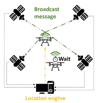
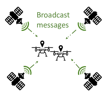
(a)	(b)

Figure 1: In (a) the traditional UTDoA approach where the tag emits the broadcast message, thus limiting the scalability of the system. In (b) the implemented DTDoA approach, where the anchors emits the messages used by the entity to localisation awareness.

This paper presents innovative DTDoA ranging techniques solving both accuracy and scalability problems of the current state of the art. Results highlight how the systems can theoretically scale to infinity (i.e., any number of assets can be tracked), improving the measurement accuracy with an error in the range of 20cm, at worst.

The main contributions of this paper are:

• The mathematical analysis of the transmission model and the characterisation of the source of uncertainties to improve the system accuracy;

• The validation of the mathematical model exploiting low-cost COTS UWB radios.

The rest of the paper is organised as follows. Section II present and discuss the mathematical model of the implemented DTDoA ranging scheme. In Section III system uncertainties and sources of error are discussed and analysed. Experimental results and evaluation are presented in Section IV. Section V closes this work with final remarks and possible future improvements.

II Models

In this section we are going to present the mathematical model of the proposed LPS. To this end, we consider an environment with a master UWB, a set of $n$ anchors $\mathbf{a}_{i}$ and a tag. We can thus denote $t$ as the actual, ideal time and with $\tau$ the time measurement from either the master $\tau^{m}(t)$; the $i$-th anchor $\mathbf{a}_{i}$ as $\tau^{i}(t)$; or the tag $\tau(t)$. Since we do not have an external time reference, we can assume that the time measurements of the master are the reference signal for the UWB positioning algorithm, following the simplified clock model presented in [34], i.e.

$$\tau^{m}(t)=o_{m}+\nu_{m}t,$$ (1)

where $o_{m}$ is the time offset of the master and $\nu_{m}=\frac{\overline{f}_{m}(t)}{f_{m}}$ the normalised clock rate with respect to the ideal time (i.e., the ratio between the instantaneous frequency of the local oscillator $\overline{f}_{m}(t)$ and the corresponding nominal value $f_{m}$, usually on the order of some part per million (ppm) [34]). Similarly, for the $i$-th anchor $\mathbf{a}_{i}$ we have

$$\tau^{i}(t)=o_{i}+\nu_{i}t,$$ (2)

where $o_{i}$ and $\nu_{i}$ are the $i$-th offset and clock rate of the time of the anchors with respect to the ideal time. Finally, for the tag we have

$$\tau(t)=o+\nu t.$$ (3)

II-A Anchors clock analysis

The main idea underlying this approach is that no message exchange should be carried out from the tag to the anchors, but only from the anchors to the tag. This to ensure infinite scalability in terms of trackable number of tags. In the ideal case, the quantities $o_{i}$, $\nu_{i}$ (with $i=1,\dots,n$) in (2) with respect to the master reference time are retrieved through the following synchronisation algorithm: starting at a generic time $\overline{t}$, the master anchor sends two messages $\tau^{m}(\overline{t})$ and $\tau^{m}(\overline{t}+\Delta_{i,m})$ to $\mathbf{a}_{i}$, whose timestamps at the receiving side are $\tau^{i}(\overline{t}+\delta_{i,m})$ and $\tau^{i}(\overline{t}+\Delta_{i,m}+\delta_{i,m})$, where $\delta_{i,m}$ is the Time of Flight (ToF) from the master to the anchor. By denoting with $[x_{m},y_{m}]^{T}$ and $\mathbf{a}_{i}=[x_{i},y_{i}]^{T}$ respectively the master and the anchor known Cartesian coordinates in the $X_{w}\times Y_{w}$ plane with respect to a fixed reference frame $\langle W\rangle=\{X_{w},Y_{w},Z_{w}\}$, it turns out that

$$\rho_{i,m}=\|[x_{m},y_{m}]^{T}-\mathbf{a}_{i}\|=\sqrt{(x_{m}-x_{i})^{2}+(y_{m}-y_{i})^{2}},$$

is the distance among the two anchors (where $\|\cdot\|$ is the usual Euclidean norm). Therefore, assuming that $c$ is the known propagation speed of the radio frequency signal in LOS conditions, we have that $\delta_{i,m}$ can be obtained as

$$\delta_{i,m}=\frac{\rho_{i,m}}{c}.$$ (4)

As a consequence, using (1) and (2) we can derive the relative clock rate

$$\overline{\nu}_{i,m}=\frac{\nu_{i}}{\nu_{m}}=\frac{\tau^{i}(\overline{t}+\Delta_{i,m}+\delta_{i,m})-\tau^{i}(\overline{t}+\delta_{i,m})}{\tau^{m}(\overline{t}+\Delta_{i,m})-\tau^{m}(\overline{t})},$$ (5)

and the relative offset

$$\tau^{i}(\overline{t}+\delta_{i,m})-\overline{\nu}_{i,m}\tau^{m}(\overline{t})-\delta_{i,m}=$$ (6)

$$=o_{i}-\overline{\nu}_{i,m}o_{m}-(1-\nu_{i})\delta_{i,m}=\overline{o}_{i,m}=$$

$$=\tau^{i}(\overline{t}+\Delta_{i,m}+\delta_{i,m})-\overline{\nu}_{i,m}\tau^{m}(\overline{t}+\Delta_{i,m})-\delta_{i,m}.$$

By assuming that the clock rates $\nu_{m}$ and $\nu_{i}$ are approximately constant among two synchronisation periods (usually executed every tens of seconds), and that the master and the anchors do not change their relative positions (i.e., the ToF $\delta_{i,m}$ is constant), we can derive that the relative offset $\overline{o}_{i,m}$ is constant as well. Furthermore, the term $(1-\nu_{i})\delta_{i,m}$ is usually negligible with respect to the relative offset between the master and the anchor. In turns, by using $\overline{\nu}_{i,m}$ – representing the correction factor that transforms the timestamped measured quantities in master time-scale into the $i$-th anchor time-scale – a generic timestamp $\tau^{i}(t)$ of an anchor can be translated to the master time-scale using (1) and

$$\frac{\tau^{i}(t)-\overline{o}_{i,m}}{\overline{\nu}_{i,m}}=o_{m}+\nu_{m}t+\frac{1-\nu_{i}}{\overline{\nu}_{i,m}}\delta_{i,m}=\tau^{m}(t)+e_{i,m}.$$ (7)

II-B Tags clock analysis

Due to the DTDoA approach used, also tag’s clock have to be corrected. Let’s consider the tag at time $t$ be in position $\mathbf{p}(t)=[x(t),y(t)]^{T}$ in $\langle W\rangle$. By denoting with

$$\rho_{i}(t)=\|\mathbf{p}(t)-\mathbf{a}_{i}\|=\sqrt{(x(t)-x_{i})^{2}+(y(t)-y_{i})^{2}},$$

the actual distance between the tag and the $i$-th anchor, we have that the ToF $\delta_{i}(t)$ is given by (4) when $\rho_{i,m}$ is substituted with $\rho_{i}(t)$. Therefore, considering that the $i$-th anchor sends two timestamped messages to the tag at time $t_{i}$ and $t_{i}+\Delta_{i}$, respectively, by using (7) we get that $\tau^{i}(t_{i})=\tau^{m}(t_{i})+e_{i,m}$ and $\tau^{i}(t_{i}+\Delta_{i})=\tau^{m}(t_{i}+\Delta_{i})+e_{i,m}$). These two messages will be received by tag time-scale at $\tau(t_{i}+\delta_{i}(t_{i}))$ and $\tau(t_{i}+\Delta_{i}+\delta_{i}(t_{i}+\Delta_{i}))$.

Considering the motion of the tag, that can be expressed as

$$\mathbf{p}(t+\Delta_{t})=\mathbf{p}(t)+\Delta_{t}\begin{bmatrix}v_{x}(t)\\ v_{y}(t)\end{bmatrix}=\mathbf{p}(t)+\Delta_{t}\mathbf{v}(t),$$

a first-order discrete time kinematics with a velocity $\mathbf{v}(t)$, we have

$$\rho_{i}(t_{i}+\Delta_{i})=\|\mathbf{p}(t_{i})+\Delta_{i}\mathbf{v}(t_{i})-\mathbf{a}_{i}\|,$$

which of course depends on the velocity vector $\mathbf{v}(t_{i})$. However, an upper bound can be found noticing that the maximum increase (or decrease) of the distance takes place when $\mathbf{v}(t_{i})$ is directed towards the anchor $\mathbf{a}_{i}$, i.e., along the direction $\mathbf{u}_{i}(t)=[x(t)-x_{i},y(t)-y_{i}]^{T}$. In such a case, denoting with $d_{i}(\Delta_{i})=\|\Delta_{i}\mathbf{v}(t_{i})\|$ the tag displacement taking place at time $t_{i}$ in the period $\Delta_{i}$, we have that

$$\rho_{i}(t_{i})-d_{i}(\Delta_{i})\mathbf{u}_{i}(t_{i})\leq\rho_{i}(t_{i}+\Delta_{i})\leq\rho_{i}(t_{i})+d_{i}(\Delta_{i})\mathbf{u}_{i}(t_{i}),$$

which yields for the ToF in (4) to

$$\delta_{i}(t_{i})-\frac{d_{i}(\Delta_{i})}{c}\mathbf{u}_{i}(t_{i})\leq\delta_{i}(t_{i}+\Delta_{i})\leq\delta_{i}(t_{i})+\frac{d_{i}(\Delta_{i})}{c}\mathbf{u}_{i}(t_{i}).$$ (8)

For what concerns the TDoA, the last missed ingredients is the synchronisation algorithm between the tag and the anchor $\mathbf{a}_{i}$. To this end, we used an algorithm that is the same of (5), i.e.,

$$\frac{\tau(t_{i}+\Delta_{i}+\delta_{i}(t_{i}+\Delta_{i}))-\tau(t_{i}+\delta_{i}(t_{i}))}{\frac{\tau^{i}(t_{i}+\Delta_{i})-\overline{o}_{i,m}}{\overline{\nu}_{i,m}}-\frac{\tau^{i}(t_{i})-\overline{o}_{i,m}}{\overline{\nu}_{i,m}}}=$$ (9)

$$=\frac{\tau(t_{i}+\Delta_{i}+\delta_{i}(t_{i}+\Delta_{i}))-\tau(t_{i}+\delta_{i}(t_{i}))}{\tau^{m}(t_{i}+\Delta_{i})-\tau^{m}(t_{i})}=$$

$$=\frac{\nu(\Delta_{i}+\alpha\frac{d_{i}(\Delta_{i})}{c}\mathbf{u}_{i}(t_{i}))}{\nu_{m}\Delta_{i}}=\overline{\nu}_{m},$$

where

$$\overline{\nu}_{m}=\frac{\nu}{\nu_{m}}\left(1+\alpha\frac{d_{i}(\Delta_{i})\mathbf{u}_{i}(t_{i})}{c\Delta_{i}}\right),$$

and $\alpha\in[-1,1]$.

II-C Indoor GPS TDoA

The UTDoA relies on an implicit event: all the anchors receive a tag’s generated broadcast message that acts as an implicit synchronisation event. In the case of an indoor GPS-like system with unbounded scalability – like the proposed DTDoA – the messages are transmitted from anchors side to the tags side; meaning that a synchronisation event cannot be defined. Strictly speaking, if such a possibility would exist, the master and anchors would send their packets simultaneously at time $t_{m}$. The tag would then measure the difference in reception times as $\tau(t_{m}+\delta_{m}(t_{m}))$ and $\tau(t_{m}+\delta_{i}(t_{m}))$ and, hence be able to compute the TDoA as

$$c\left[\tau(t_{m}+\delta_{i}(t_{m}))-\tau(t_{m}+\delta_{m}(t_{m}))\right]=$$ (10)

$$=c\nu(\delta_{i}(t_{m})-\delta_{m}(t_{m}))=\nu(\rho_{i}-\rho_{m}),$$

$\forall i=1,\dots,n$. Notice that such a measure is only affected by the relative clock rate $\nu$, which is of course negligible since it generates an error in the order of some micrometers.

Since such a synchronised event cannot be generated (the anchor will transmit at slightly different time instants and the tag cannot receive all the messages at once), the syntonisation between tags and anchors (i.e., estimation of the relative clock rates) cannot neglected. Let’s considering a system composed by a master, a number of anchors $i$ and a tag. At time $t_{m}$ a broadcast message is transmitted from the master, followed by a second message at time $t_{m}+\Delta_{m}$. The tag timestamps the messages at reception times, denoted as $\tau(t_{m}+\delta_{m}(t_{m}))$ and $\tau(t_{m}+\Delta_{m}+\delta_{m}(t_{m}+\Delta_{m}))$ Finally the tag stores the two transmission timestamp encapsulated inside the broadcast message, defined as $\tau^{m}(t_{m})$ and $\tau^{m}(t_{m}+\Delta_{m})$. The same happens with the anchor $i$ transmitting at time $t_{i}$ and $t_{i}+\Delta_{i}$, with tag’s timestamped reception times $\tau(t_{i}+\delta_{i}(t_{i}))$ and $\tau(t_{i}+\Delta_{i}+\delta_{i}(t_{i}+\Delta_{i}))$, and the two transmitted timestamps $\frac{\tau^{i}(t_{i})-\overline{o}_{i,m}}{\overline{\nu}_{i,m}}$ and $\frac{\tau^{i}(t_{i}+\Delta_{i})-\overline{o}_{i,m}}{\overline{\nu}_{i,m}}$, as corrected anchor clock in master time scale using (7). It is then possible to compute at the tag side the relative clock rates $\overline{\nu}_{m}$ using (9) (that explaining the necessity to send/receive two messages) and a function $g(\Delta_{i,m})$ of the protocol time interval $\Delta_{i,m}=t_{i}-t_{m}$ by means of the clock model (1) as

$$g(\Delta_{i,m})=\overline{\nu}_{m}\left(\frac{\tau^{i}(t_{i})-\overline{o}_{i,m}}{\overline{\nu}_{i,m}}-\tau^{m}(t_{m})\right)=$$ (11)

$$=\overline{\nu}_{m}(\tau^{m}(t_{i})-\tau^{m}(t_{m})+e_{i,m})=$$

$$=\overline{\nu}_{m}\nu_{m}(t_{i}-t_{m})+\overline{\nu}_{m}e_{i,m}=$$

$$=\nu\Delta_{i,m}+\nu\alpha\frac{d_{i}(\Delta_{i,m})\mathbf{u}_{i}(t_{m})}{c}+\overline{\nu}_{m}e_{i,m}.$$

By defining the corresponding tag timestamps and the clock model (3) as

$$\tau(t_{i}+\delta_{i}(t_{i}))-\tau(t_{m}+\delta_{m}(t_{m}))=$$ (12)

$$=\nu(\delta_{i}(t_{i})-\delta_{m}(t_{m}))+\nu(t_{i}-t_{m})=$$

$$=\nu(\delta_{i}(t_{m}+\Delta_{i,m})-\delta_{m}(t_{m}))+\nu\Delta_{i,m},$$

and considering (8) as

$$\delta_{i}(t_{m}+\Delta_{i,m})=\delta_{i}(t_{m})+\alpha\frac{d_{i}(\Delta_{i,m})}{c}\mathbf{u}_{i}(t_{m}),$$

we can finally have derive the DTDoA equation:

$$c\left[\tau(t_{i}+\delta_{i}(t_{i}))-\tau(t_{m}+\delta_{m}(t_{m}))-g(\Delta_{i,m})\right]=$$ (13)

$$=\nu(\rho_{i}-\rho_{m})-c\overline{\nu}_{m}e_{i,m}.$$

computed using (4) and (11).

Those quantities can be equivalently computed for the delayed messages, by considering $\tau^{m}(t_{m}+\Delta_{m})$ and $\tau^{i}(t_{i}+\Delta_{i})$ in (11); and $\tau(t_{m}+\Delta_{m}+\delta_{m}(t_{m}+\Delta_{m}))$ and $\tau(t_{i}+\Delta_{i}+\delta_{i}(t_{i}+\Delta_{i}))$ in (12). Of course, comparing (13) and (10), we can notice that in the presence of multiple time sources (i.e., having $i$ anchors) induces potential errors stemming from the imperfect synchronisation with the master, highlighted in (7), which is, unfortunately unavoidable.

III Uncertainties

The main source of uncertainties – neglecting the effects of ageing or the drift changes induced by harsh environmental conditions (e.g., mechanical vibrations or temperature effects [34]) – is related to timestamping accuracy operation. Albeit those effects can be dramatically reduced by implementing double consecutive message transmissions (i.e., the timestamp is acquired when the message is sent, and then transmitted in a second message, as in [34]), the effect cannot be entirely removed. As a consequence, by denoting with $\eta$ the generic timestamping uncertainty affecting each clock in the network, we can rewrite the clock models as

$${{\tau^{m}}^{\star}}(t) =o_{m}+\nu_{m}t+\eta_{m}(t)=\tau^{m}(t)+\eta_{m}(t),$$ (14)

$${{\tau^{i}}^{\star}}(t) =o_{i}+\nu_{i}t+\eta_{i}(t)=\tau^{i}(t)+\eta_{i}(t),$$

$${{\tau}^{\star}}(t) =o+\nu t+\eta(t)=\tau(t)+\eta(t),$$

where we use the superscript ${{\cdot}^{\star}}$ to denote each measurement result. It worth to be noted that we implicitly assume that the measurement uncertainties $\eta_{m}(t)$, $\eta_{i}(t)$ and $\eta(t)$ are random variables generated by white, stationary and zero mean processes with variances $\sigma_{\eta_{m}}^{2}$, $\sigma_{\eta_{i}}^{2}$ and $\sigma_{\eta}^{2}$, respectively.

By assuming a first-order Taylor approximation for the uncertainty, the relative clock rates $\overline{\nu}_{i,m}$ in (5), when computed with (14) becomes

$$\frac{{{\tau^{i}}^{\star}}(\overline{t}+\Delta_{i,m}+\delta_{i,m})-{{\tau^{i}}^{\star}}(\overline{t}+\delta_{i,m})}{{{\tau^{m}}^{\star}}(\overline{t}+\Delta_{i,m})-{{\tau^{m}}^{\star}}(\overline{t})}\approx\overline{\nu}_{i,m}+\beta={{\overline{\nu}_{i,m}}^{\star}},$$

having the uncertainty mean $\mu_{\beta}=\text{E}\left\{\beta\right\}=0$ (the $\text{E}\left\{\cdot\right\}$ is the usual expected operator) and its variance

$$\text{E}\left\{\beta^{2}\right\}=\sigma_{\beta}^{2}=\frac{2}{\nu_{m}^{2}\Delta_{i,m}^{2}}(\sigma_{\eta_{i}}^{2}+\overline{\nu}_{i,m}^{2}\sigma_{\eta_{m}}^{2}),$$

It can thus be argued that the larger the interval $\Delta_{i,m}$, the smaller the uncertainty on the indirect measurement of ${{\overline{\nu}_{i,m}}^{\star}}$. For the relative offsets $\overline{o}_{i,m}$ in (6), we have similarly

$${{\tau^{i}}^{\star}}(\overline{t}+\delta_{i,m})-{{\overline{\nu}_{i,m}}^{\star}}{{\tau^{m}}^{\star}}(\overline{t})-\delta_{i,m}\approx\overline{o}_{i,m}+\gamma(\overline{t})={{\overline{o}_{i,m}}^{\star}}(\overline{t}),$$ (15)

with mean $\mu_{\gamma}(\overline{t})=\text{E}\left\{\gamma(\overline{t})\right\}=0$ and variance

$$\sigma_{\gamma}^{2}(\overline{t})=\text{E}\left\{\gamma(\overline{t})^{2}\right\}=\left(1-2\frac{\tau^{m}(\overline{t})}{\nu_{m}\Delta_{i,m}}\right)\sigma_{\eta_{i}}^{2}+$$

$$+\overline{\nu}_{i,m}^{2}\left(1+2\frac{\tau^{m}(\overline{t})}{\nu_{m}\Delta_{i,m}}\right)\sigma_{\eta_{m}}^{2}+\tau^{m}(\overline{t})^{2}\sigma_{\beta}^{2}.$$

By using (6), we can also make use of the quantities delayed by $\Delta_{i,m}$ yielding to a similar quantity as in (15) but denoted with ${{\overline{o}_{i,m}}^{\star}}(\overline{t}+\Delta_{i,m})$. It is then possible to formulate a new estimate as

$$\hat{\overline{o}}_{i,m}=\frac{{{\overline{o}_{i,m}}^{\star}}(\overline{t})+{{\overline{o}_{i,m}}^{\star}}(\overline{t}+\Delta_{i,m})}{2}=\overline{o}_{i,m}+\overline{\gamma}(\overline{t}),$$ (16)

that is again affected by a zero mean uncertainty with variance

$$\sigma_{\overline{\gamma}}^{2}(\overline{t})=\frac{\sigma_{\eta_{i}}^{2}}{2}+\frac{\sigma_{\eta_{m}}^{2}}{2}+\tau^{m}\left(\overline{t}+\frac{\Delta_{i,m}}{2}\right)^{2}\sigma_{\beta}^{2},$$

which may or may not be more useful than (15) depending on the value of $\Delta_{i,m}$. This is a direct consequence of the fact that ${{\overline{o}_{i,m}}^{\star}}(\overline{t})$ and ${{\overline{o}_{i,m}}^{\star}}(\overline{t}+\Delta_{i,m})$ are correlated by ${{\overline{\nu}_{i,m}}^{\star}}$.

For what concerns equation (7), if the time $t$ in which the anchor time scale is converted into the master time scale is different from $\overline{t}$, $\overline{t}+\Delta_{i,m}$, $\overline{t}+\delta_{i,m}$ and $\overline{t}+\Delta_{i,m}+\delta_{i,m}$ (i.e., the times in which (5) and (6) are used), we can again use a first-order Taylor approximation to re-write (7) as

$$\frac{{{\tau^{i}}^{\star}}(t)-\hat{\overline{o}}_{i,m}}{{{\overline{\nu}_{i,m}}^{\star}}}\approx\tau^{m}(t)+e_{i,m}+\varepsilon(t).$$

Having $\text{E}\left\{\varepsilon(t)\right\}=0$ and

$$\sigma_{\varepsilon}^{2}(t) =\frac{\sigma_{\eta_{i}}^{2}}{\overline{\nu}_{i,m}^{2}}+\frac{\sigma_{\overline{\gamma}}^{2}(\overline{t})}{\overline{\nu}_{i,m}^{2}}+$$

$$+\left[\frac{(\tau^{m}(t)+e_{i,m})^{2}}{\overline{\nu}_{i,m}^{2}}-2\frac{\tau^{m}(t)+e_{i,m}}{\overline{\nu}_{i,m}^{2}}\tau^{m}(\overline{t})\right]\sigma_{\beta}^{2}.$$

allow us to compute the uncertain version of (9) as

$$\frac{{{\tau}^{\star}}(t_{i}+\Delta_{i}+\delta_{i}(t_{i}+\Delta_{i}))-{{\tau}^{\star}}(t_{i}+\delta_{i}(t_{i}))}{\frac{{{\tau^{i}}^{\star}}(t_{i}+\Delta_{i})-\hat{\overline{o}}_{i,m}}{{{\overline{\nu}_{i,m}}^{\star}}}-\frac{{{\tau^{i}}^{\star}}(t_{i})-\hat{\overline{o}}_{i,m}}{{{\overline{\nu}_{i,m}}^{\star}}}}\approx$$

$$\approx\overline{\nu}_{m}+\xi(\Delta_{i})={{\overline{\nu}_{m}}^{\star}},$$

with $\text{E}\left\{\xi(\Delta_{i})\right\}=0$ and

$$\sigma_{\xi}^{2}(\Delta_{i})=\frac{2\overline{\nu}_{m}^{2}}{\nu_{i}^{2}\Delta_{i}^{2}}\sigma_{\eta_{i}}^{2}+\frac{2}{\nu_{m}^{2}\Delta_{i}^{2}}\sigma_{\eta}^{2}+\frac{\overline{\nu}_{m}^{2}}{\nu_{i,m}^{2}}\sigma_{\beta}^{2}.$$

Similarly, to compute the noisy protocol interval in (11), we have

$${{g}^{\star}}(\Delta_{i,m}) ={{\overline{\nu}_{m}}^{\star}}\left(\frac{{{\tau^{i}}^{\star}}(t_{i})-\hat{\overline{o}}_{i,m}}{{{\overline{\nu}_{i,m}}^{\star}}}-{{\tau^{m}}^{\star}}(t_{m})\right)\approx$$

$$\approx g(\Delta_{i,m})+\varphi(t_{i},t_{m}).$$

In this case $\text{E}\left\{\varphi(t_{i},t_{m})\right\}=0$ and

$$\sigma_{\varphi}^{2}(t_{i},t_{m})=\overline{\nu}_{m}^{2}(\sigma_{\varepsilon}^{2}(t_{i})+\sigma_{\nu_{m}}^{2})+$$

$$+\frac{2\overline{\nu}_{m}^{2}}{\nu_{m}\Delta_{i}}(\nu_{m}\Delta_{i,m}+e_{i,m})(\sigma_{\varepsilon}^{2}(t_{i})-\sigma_{\varepsilon}(t_{i},t_{i}+\Delta_{i}))+$$

$$+(\nu_{m}\Delta_{i,m}+e_{i,m})^{2}\sigma_{\xi}^{2}(\Delta_{i}),$$

where $\sigma_{\varepsilon}(t_{i},t_{i}+\Delta_{i}))$ is the correlation between the uncertainties $\varepsilon(t_{i})$ and $\varepsilon(t_{i}+\Delta_{i})$ leading to

$$\text{E}\left\{\varepsilon(t_{i})\varepsilon(t_{i}+\Delta_{i})\right\}=\frac{(\tau^{m}(t_{i})+e_{i,m})(\tau^{m}(t_{i}+\Delta_{i})}{\overline{\nu}_{i,m}^{2}}\sigma_{\beta}^{2}+$$

$$+\frac{\sigma_{\overline{\gamma}}^{2}(\overline{t})}{\overline{\nu}_{i,m}^{2}}-\frac{\tau^{m}(t_{i})+\tau^{m}(t_{i}+\Delta_{i})+2e_{i,m}}{\overline{\nu}_{i,m}^{2}}\tau^{m}\left(\overline{t}+\frac{\Delta_{i,m}}{2}\right)\sigma_{\beta}^{2}.$$

We are now ready to conclude the uncertainty analysis by computing the final DTDoA relation (13) once the measured quantities in (14) are used:

$$c\left[{{\tau}^{\star}}(t_{i}+\delta_{i}(t_{i}))-{{\tau}^{\star}}(t_{m}+\delta_{m}(t_{m}))-{{g}^{\star}}(\Delta_{i,m})\right]=$$

$$=\nu(\rho_{i}-\rho_{m})-c\overline{\nu}_{m}e_{i,m}+\lambda(t_{i},t_{m}),$$

resulting in an overall uncertainty with mean $\text{E}\left\{\lambda(t_{i},t_{m})\right\}=0$ and variance

$$\sigma_{\lambda}^{2}(t_{i},t_{m})=c^{2}\left[2\left(1+\frac{\nu_{m}\Delta_{i,m}+e_{i,m}}{\nu_{m}\Delta_{i}}\right)\sigma_{\eta}^{2}+\sigma_{\varphi}^{2}(t_{i},t_{m})\right].$$ (17)

III-A Numerical analysis

In this section we present the simulations results about the validity of the uncertainty analysis presented in the previous subsection. The first simulation analyse the tightness of the approximations of the uncertainties introduced by the first-order Taylor linearisation. Figure 2 presents the absolute relative error, expressed in percentage, between the theoretical values of the mean $\mu_{\gamma}(\overline{t})$ and the standard deviation $\sigma_{\gamma}(\overline{t})$ in (15) for the uncertainty $\gamma(\overline{t})$, with respect to the values obtained through $10000$ Monte Carlo Simulations, here denoted with $\mu_{\gamma}^{MC}(\overline{t})$ and $\sigma_{\gamma}^{MC}(\overline{t})$:

$$\mu_{\gamma}^{\%}(\overline{t})=100\frac{|\mu_{\gamma}(\overline{t})-\mu_{\gamma}^{MC}(\overline{t})|}{\mu_{\gamma}^{MC}(\overline{t})},$$

and

$$\sigma_{\gamma}^{\%}(\overline{t})=100\frac{|\sigma_{\gamma}(\overline{t})-\sigma_{\gamma}^{MC}(\overline{t})|}{\sigma_{\gamma}^{MC}(\overline{t})},$$

respectively.

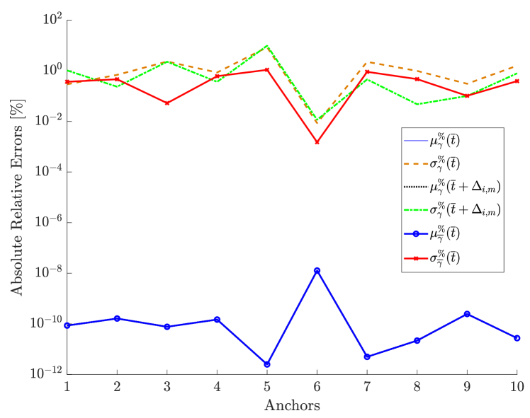
Figure 2: Absolute relative error of the theoretical approximations with respect to Monte Carlo simulations for the random variables $\gamma(\overline{t})$, $\gamma(\overline{t}+\Delta_{i,m})$ and $\overline{\gamma}(\overline{t})$.

The Monte Carlo simulations assume $10$ anchors (on the abscissa of Figure 2) with randomly generated clock time offsets, clock rates, positions, delays $\Delta_{i}$ and $\Delta_{i,m}$, having zero-mean, Gaussian time stamping uncertainties $\eta_{m}(t)$, $\eta_{i}(t)$, and $\eta(t)$, with a maximum value of plus/minus $15.65$ ps (i.e., one clock tick, as per the available hardware, see Section IV). As can be seen from Figure 2, whatever uncertainty is considered, i.e. $\gamma(\overline{t})$, $\gamma(\overline{t}+\Delta_{i,m})$ or the average of the two $\overline{\gamma}(\overline{t})$ reported in (16), the theoretical analysis matches remarkably well with the simulations (the mean, for example, are all overlapped with negligible errors in Figure 2). Similar results are obtained for all the other quantities, here not reported for space limits.

Of course, the approximation becomes less accurate when the timestamping uncertainties are uniformly distributed between plus/minus $15.65$ ps, as reported in Figure 3 that presents the DTDoA uncertainties in (17) for the anchor $\mathbf{a}_{1}$.

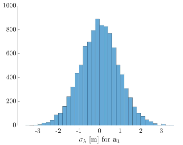
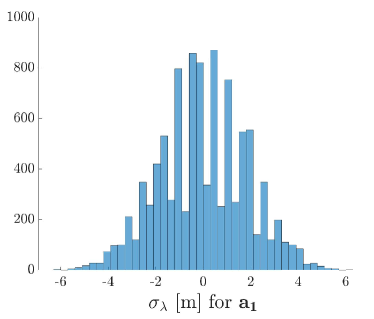
(a)	(b)

Figure 3: Distribution of the DTDoA uncertainties $\sigma_{\lambda}^{2}(t_{i},t_{m})$ in (17) in the case of (a) Gaussian and (b) Uniform timestamping uncertainties.

IV Experimental Results

To evaluate and validate the statistical model discussed in the previous section, we have implemented the proposed DTDoA algorithm using UWB radios. UWB radio transmission is based upon impulse radio (IR) schemes. The pulses being applied in IR have a very short temporal duration (typically in order of nanoseconds), which results in an ultra-wide band spectrum [35]. This very large spectrum allows to achieve excellent time and spatial resolution by evaluating the Channel Impulse Response (CIR) of the signal.

IV-A Hardware Implementation

To implement our LPS, we decided to use the commercial-off-the-shelf (COTS) Decawave DWM1001 SoM, which attracted many interests for implementing indoor positioning systems [36]. The DWM1001 is a compact module that integrates both a low power nRF52832 MCU and the Decawave DW1000 UWB transceiver. It also integrates RF circuitry, an UWB antenna and a motion sensor for sensor fusion applications [37].

The DW1000 chip is an IEEE 802.15.4-2011 [38] compliant UWB transceiver which can operate on 6 different frequency bands with centre frequencies between 3.5 to 6.5 GHz and a bandwidth of 500 or 900 MHz. It provides the possibility of ranging measurements and retrieving the measured CIR. The chip also offers three different data rates: 110 kbps, 850 kbps and 6.8 Mbps.

The DW1000 clocking scheme is based on 3 main circuits; crystal oscillator (trimmed in production to reduce the initial frequency error to approximately 3 ppm), Clock Phase-Locked Loop (PLL) and RF PLL. The on-chip oscillator is designed to operate at a frequency of 38.4 MHz. This clock is then used as the reference input to the two on-chip PLLs. The clock PLL generates a 63.8976 GHz reference clock required by the digital backend for signal processing. The RF PLL generates the clock for the receive and transmit chain. The DW1000 automatically timestamps transmitted and received frames with a precision of 40-bit. In turns, working at a nominal 64 GHz resolution, packets are timestamped with a 15.65 ps event timing precision.

During the experimental tests, the DWM1001 SoM was configured to use UWB Channel 5 ($f_{c}=6489.6$ MHz, $BW=499.2$ MHz), a preamble length of 128 symbols, the highest Pulse Rate $PR=64$ MHz, and the highest Data Rate$DR=6.8$ Mbps.

IV-B Network infrastructure

To exploit the UWB protocol to implement an LPS, a specific number of DWM1001 module must be programmed to act as anchors and, hence, provide a reference infrastructure for the tags. In our case, the reference infrastructure comprises six reference anchors mounted on the wall of our laboratory. Each anchor is mainly composed of a Raspberry PI 3 and a DWM1001 module. Finally, data sharing and acquisition is implemented by leveraging the MQTT protocol. In this way, both anchors and tags data can be retrieved easily also by a remote system.

IV-C Positioning Results

To evaluate and characterise the statistical properties of the developed positioning infrastructure, two experiments were conducted. The first test is done in static conditions with a tag positioned in two known locations. Figure 4 depicts the histogram of the estimation error along the $X_{w}$ and $Y_{w}$ axis, i.e. $\tilde{x}_{k}=\hat{x}_{k}-x_{k}$ and $\tilde{y}_{k}=\hat{y}_{k}-y_{k}$, respectively, for the two test positions over $30000$ repeated measurements.

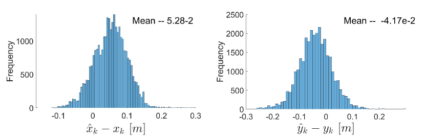
Test position 1

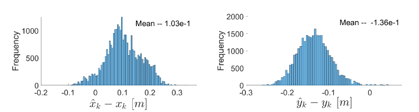
Test position 2

Figure 4: Histogram of the error for the test positions 1 and 2 along the $X_{w}$ (left) and $Y_{w}$ (right) reference axes over $30000$ repeated measurements.

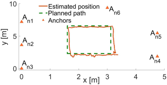
Figure 5: Walking test

As can be noted, they present a non-zero mean Gaussian distribution due to the effects of angle-dependent UWB pulse distortion and the path overlap [39]. Moreover, the measure is also subjected to the anchors distribution in the testing room that may cause reflections due to the presence of metallic objects. Nonetheless, the precision is below the claimed $20$ cm of error.

The second test was conducted while moving the receiver along a planned path to evaluate the effectiveness of the infrastructure, both for tracking or navigation purposes. The result is reported in Figure 5 where the green dashed line represents the planned path. The asymmetry in the estimated positions, can be explained using the Position Dilution of Precision (PDoP) (see Figure 6 for the PDoP map of the adopted environment).

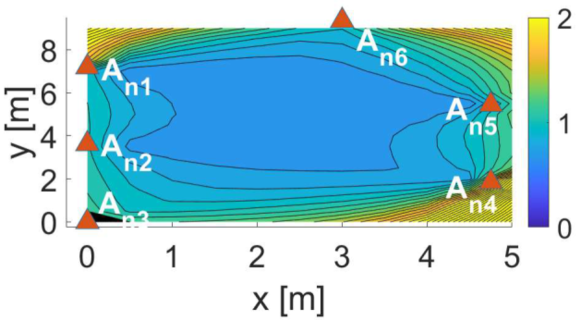
Figure 6: PDoP map for the actual anchors distributions for the experiment in Figure 5.

Although the PDoP does not consider complex non-line-of-sight and multipath problems, it can be considered a valid simple metric to express positioning accuracy [40].

As described in Section I, the main purpose of the presented solution is to determine the position of an unlimited number of assets (e.g., robots) inside the environment. As presented in Figure 7, which shows the execution time needed for receiving all the messages from the reference anchors, the positioning routine is scheduled at the receiver side.

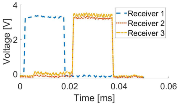
Figure 7: Three tags complete independently their position estimation phase. The graph reports the voltage measured from a pin of the GPIO, which is rose when a tag is engaged into the positioning phase.

In this example, Receiver 1 completes its pose estimation before the others, while the second and the third receivers estimate their position simultaneously. This confirms that the system allows simultaneous position estimates from different tags, thus empirically prove that the system can scale up to infinity.

V Conclusion

This paper presents the solution to the scalability problem of LPSs. The introduced DTDoA scheme enables the possibility to supply the pose information to an infinite number of entities and robots endowed with an UWB receiver. The source of uncertainties analysis highlighted the critical points for the DTDoA scheme and guided the development of an LPS with a maximum absolute position error below $20$ cm. The maximum pose information update rate reached in this work is $67$ Hz. In future work, we investigate alternative downlink schemes to increase the update rate of the localisation, removing the limit given by the number of active anchors. Another goal is to increase the accuracy of localisation system exploiting hybrid techniques to take care of the non-line-of-sight and multipath problems.

References

- [1] R. Siegwart and I. R. Nourbakhsh, Introduction to Autonomous Mobile Robots. Scituate, MA, USA: Bradford Company, 2004.
- [2] N. Saeed, H. Nam, T. Y. Al-Naffouri, and M.-S. Alouini, “A state-of-the-art survey on multidimensional scaling-based localization techniques,” IEEE Communications Surveys Tutorials, vol. 21, no. 4, pp. 3565–3583, 2019.
- [3] J. Karl, Celestial navigation in the GPS age. Paradise Cay Publications, 2007.
- [4] G. Seco-Granados, J. López-Salcedo, D. Jiménez-Baños, and G. López-Risueño, “Challenges in indoor global navigation satellite systems: Unveiling its core features in signal processing,” IEEE Signal Processing Magazine, vol. 29, no. 2, pp. 108–131, 2012.
- [5] M. Maheepala, A. Z. Kouzani, and M. A. Joordens, “Light-based indoor positioning systems: A review,” IEEE Sensors Journal, vol. 20, no. 8, pp. 3971–3995, 2020.
- [6] T. Kim Geok, K. Zar Aung, M. Sandar Aung, M. Thu Soe, A. Abdaziz, C. Pao Liew, F. Hossain, C. P. Tso, and W. H. Yong, “Review of indoor positioning: Radio wave technology,” Applied Sciences, vol. 11, no. 1, 2021. [Online]. Available: https://www.mdpi.com/2076-3417/11/1/279
- [7] P. Pascacio, S. Casteleyn, J. Torres-Sospedra, E. S. Lohan, and J. Nurmi, “Collaborative indoor positioning systems: A systematic review,” Sensors, vol. 21, no. 3, 2021. [Online]. Available: https://www.mdpi.com/1424-8220/21/3/1002
- [8] Y. YIN, Y. Zeng, X. Chen, and Y. Fan, “The internet of things in healthcare: An overview,” Journal of Industrial Information Integration, vol. 1, pp. 3–13, 2016. [Online]. Available: https://www.sciencedirect.com/science/article/pii/S2452414X16000066
- [9] S. de Miguel-Bilbao, J. Roldán, J. García, F. López, P. García-Sagredo, and V. Ramos, “Comparative analysis of indoor location technologies for monitoring of elderly,” in 2013 IEEE 15th International Conference on e-Health Networking, Applications and Services (Healthcom 2013), 2013, pp. 320–323.
- [10] K. Ren, J. Karlsson, M. Liuska, M. Hartikainen, I. Hansen, and G. H. Jørgensen, “A sensor-fusion-system for tracking sheep location and behaviour,” International Journal of Distributed Sensor Networks, vol. 16, no. 5, p. 1550147720921776, 2020. [Online]. Available: https://doi.org/10.1177/1550147720921776
- [11] S. Koompairojn, C. Puitrakul, T. Bangkok, N. Riyagoon, and S. Ruengittinun, “Smart tag tracking for livestock farming,” in 2017 10th International Conference on Ubi-media Computing and Workshops (Ubi-Media), 2017, pp. 1–4.
- [12] E. Sun and R. Ma, “The uwb based forklift trucks indoor positioning and safety management system,” in 2017 IEEE 2nd Advanced Information Technology, Electronic and Automation Control Conference (IAEAC), 2017, pp. 86–90.
- [13] B. Ivsic, J. Bartolic, Z. Sipus, and J. Babic, “Uwb propagation characteristics of human-to-robot communication in automated collaborative warehouse,” in 2020 IEEE International Symposium on Antennas and Propagation and North American Radio Science Meeting, 2020, pp. 1125–1126.
- [14] H. Obeidat, W. Shuaieb, O. Obeidat, and R. Abd-Alhameed, “A review of indoor localization techniques and wireless technologies,” Wireless Personal Communications, vol. 119, no. 1, pp. 289–327, Jul 2021. [Online]. Available: https://doi.org/10.1007/s11277-021-08209-5
- [15] M. S. Mozamir, R. B. A. Bakar, and W. I. S. W. Din, “Indoor localization estimation techniques in wireless sensor network: A review,” in 2018 IEEE International Conference on Automatic Control and Intelligent Systems (I2CACIS), 2018, pp. 148–154.
- [16] J. S. Willners, L. Toohey, and Y. Petillot, “Improving acoustic range-only localisation by selection of transmission time,” in OCEANS 2019 - Marseille, 2019, pp. 1–6.
- [17] M. Faisal, R. Hedjar, M. Alsulaiman, K. Al-Mutabe, and H. Mathkour, “Robot localization using extended kalman filter with infrared sensor,” in 2014 IEEE/ACS 11th International Conference on Computer Systems and Applications (AICCSA), 2014, pp. 356–360.
- [18] C. Zhang and X. Zhang, “Visible light localization using conventional light fixtures and smartphones,” IEEE Transactions on Mobile Computing, vol. 18, no. 12, pp. 2968–2983, 2019.
- [19] F. Bernardini, A. Buffi, D. Fontanelli, D. Macii, V. Magnago, M. Marracci, A. Motroni, P. Nepa, and B. Tellini, “Robot-based Indoor Positioning of UHF-RFID Tags: the SAR Method with Multiple Trajectories,” IEEE Trans. on Instrumentation and Measurement, vol. 70, pp. 1–15, 2021, available on line.
- [20] K. Lorvannger, D. Lakanchanh, T. Tiengthong, and S. Promwong, “Wlan localization measurement and analysis using rss and toa positioning methods,” in 2018 Global Wireless Summit (GWS), 2018, pp. 319–322.
- [21] J. A. del Peral-Rosado, R. Raulefs, J. A. López-Salcedo, and G. Seco-Granados, “Survey of cellular mobile radio localization methods: From 1g to 5g,” IEEE Communications Surveys Tutorials, vol. 20, no. 2, pp. 1124–1148, 2018.
- [22] A. Alarifi, A. Al-Salman, M. Alsaleh, A. Alnafessah, S. Al-Hadhrami, M. A. Al-Ammar, and H. S. Al-Khalifa, “Ultra wideband indoor positioning technologies: Analysis and recent advances,” Sensors, vol. 16, no. 5, 2016. [Online]. Available: https://www.mdpi.com/1424-8220/16/5/707
- [23] M. Ivanić and I. Mezei, “Distance estimation based on rssi improvements of orientation aware nodes,” in 2018 Zooming Innovation in Consumer Technologies Conference (ZINC), 2018, pp. 140–143.
- [24] M. Nardello, L. Santoro, F. Pilati, and D. Brunelli, “Preventing covid-19 contagion in industrial environments through anonymous contact tracing,” in 2021 IEEE International Workshop on Metrology for Industry 4.0 IoT (MetroInd4.0 IoT), 2021, pp. 99–104.
- [25] W. Liu, Y. Xiong, X. Zong, and W. Siwei, “Trilateration positioning optimization algorithm based on minimum generalization error,” in 2018 IEEE 4th International Symposium on Wireless Systems within the International Conferences on Intelligent Data Acquisition and Advanced Computing Systems (IDAACS-SWS), 2018, pp. 154–157.
- [26] H. Hu, M. Wang, M. Fu, and Y. Yang, “Sound source localization sensor of robot for tdoa method,” in 2011 Third International Conference on Intelligent Human-Machine Systems and Cybernetics, vol. 2, 2011, pp. 19–22.
- [27] R. Peng and M. L. Sichitiu, “Angle of arrival localization for wireless sensor networks,” in 2006 3rd Annual IEEE Communications Society on Sensor and Ad Hoc Communications and Networks, vol. 1, 2006, pp. 374–382.
- [28] C. L. Sang, M. Adams, T. Hörmann, M. Hesse, M. Porrmann, and U. Rückert, “An analytical study of time of flight error estimation in two-way ranging methods,” in 2018 International Conference on Indoor Positioning and Indoor Navigation (IPIN), 2018, pp. 1–8.
- [29] V. Magnago, P. Corbalán, G. Picco, L. Palopoli, and D. Fontanelli, “Robot Localization via Odometry-assisted Ultra-wideband Ranging with Stochastic Guarantees,” in Proc. IEEE/RSJ International Conference on Intelligent Robots and System (IROS). Macao, China: IEEE, Nov. 2019, pp. 1607–1613.
- [30] Y. Cheng and T. Zhou, “Uwb indoor positioning algorithm based on tdoa technology,” in 2019 10th International Conference on Information Technology in Medicine and Education (ITME), 2019, pp. 777–782.
- [31] P. Corbalán, G. P. Picco, and S. Palipana, “Chorus: Uwb concurrent transmissions for gps-like passive localization of countless targets,” in 2019 18th ACM/IEEE International Conference on Information Processing in Sensor Networks (IPSN), 2019, pp. 133–144.
- [32] R. Zandian and U. Witkowski, “Robot self-localization in ultra-wideband large scale multi-node setups,” in 2017 14th Workshop on Positioning, Navigation and Communications (WPNC), 2017, pp. 1–6.
- [33] M. Pelka and H. Hellbrück, “S-tdoa — sequential time difference of arrival — a scalable and synchronization free approach forl positioning,” in 2016 IEEE Wireless Communications and Networking Conference, 2016, pp. 1–6.
- [34] D. Fontanelli, D. Macii, P. Wolfrumand, D. Obradovic, and G. Steindl, “A clock state estimator for ptp time synchronization in harsh environmental conditions,” in Proc. IEEE Int. Symp. on Precision Clock Synchronization for Measurement, Control and Communication (ISPCS), Munich, Germany, 12-16 Sept. 2011, pp. 99–104, Best Academic Paper Award.
- [35] I. Oppermann, M. Hämäläinen, and J. Iinatti, UWB: theory and applications. John Wiley & Sons, 2004.
- [36] J. Kulmer, S. Hinteregger, B. Großwindhager, M. Rath, M. S. Bakr, E. Leitinger, and K. Witrisal, “Using decawave uwb transceivers for high-accuracy multipath-assisted indoor positioning,” in 2017 IEEE International Conference on Communications Workshops (ICC Workshops), 2017, pp. 1239–1245.
- [37] M. Frisk and A. Nilsson, “Inertial sensor and ultra-wideband sensor fusion: Precision positioning of robot platform,” Ph.D. dissertation, 2014. [Online]. Available: http://urn.kb.se/resolve?urn=urn:nbn:se:uu:diva-231053
- [38] I. . W. Group et al., “Ieee standard for local and metropolitan area networks—part 15.4: Low-rate wireless personal area networks (lr-wpans),” IEEE Std, vol. 802, pp. 4–2011, 2011.
- [39] A. Ledergerber and R. D’Andrea, “Ultra-wideband range measurement model with gaussian processes,” in 2017 IEEE Conference on Control Technology and Applications (CCTA), 2017, pp. 1929–1934.
- [40] M. Wang, Z. Chen, Z. Zhou, J. Fu, and H. Qiu, “Analysis of the applicability of dilution of precision in the base station configuration optimization of ultrawideband indoor tdoa positioning system,” IEEE Access, vol. 8, pp. 225 076–225 087, 2020.