Episodic Policy Gradient Training

Abstract

We introduce a novel training procedure for policy gradient methods wherein episodic memory is used to optimize the hyperparameters of reinforcement learning algorithms on-the-fly. Unlike other hyperparameter searches, we formulate hyperparameter scheduling as a standard Markov Decision Process and use episodic memory to store the outcome of used hyperparameters and their training contexts. At any policy update step, the policy learner refers to the stored experiences, and adaptively reconfigures its learning algorithm with the new hyperparameters determined by the memory. This mechanism, dubbed as Episodic Policy Gradient Training (EPGT), enables an episodic learning process, and jointly learns the policy and the learning algorithm’s hyperparameters within a single run. Experimental results on both continuous and discrete environments demonstrate the advantage of using the proposed method in boosting the performance of various policy gradient algorithms.

Introduction

The current success of deep reinforcement learning relies on the ability to use gradient-based optimizations for policy and value learning (Mnih et al. 2015; Silver et al. 2017). Approaches such as policy gradient (PG) methods have achieved remarkable results in various domains including games (Mnih et al. 2016; Schulman et al. 2017; Wu et al. 2017; Fujimoto, Hoof, and Meger 2018), robotics (Kohl and Stone 2004; Peters and Schaal 2006) or even natural language processing (Ziegler et al. 2019). However, the excellent performance of PG methods is heavily dependent on tuning the algorithms’ hyperparameters (Duan et al. 2016; Zhang et al. 2021). Applying a PG method to new environments often requires different hyperparameter settings and thus retuning (Henderson et al. 2018). The large amount of hyperparameters severely prohibits machine learning practitioners from fully utilizing PG methods in different reinforcement learning environments.

As a result, there is a huge demand for automating hyperparameter selection for policy gradient algorithms, and it remains a critical part of the Automated Machine Learning (AutoML) movement (Hutter, Kotthoff, and Vanschoren 2019). Automatic hyperparameter tuning has been well explored for supervised learning. Simple methods such as grid search and random search are effective although computationally expensive (Bergstra and Bengio 2012; Larochelle et al. 2007). Other complex methods such as Bayesian Optimization (BO (Snoek, Larochelle, and Adams 2012)) and Evolutionary Algorithms (EA (Fiszelew et al. 2007)) can efficiently search for optimal hyperparameters. Yet, they still need multiple training runs, have difficulty scaling to high-dimensional settings (Rana et al. 2017) or require extensive parallel computation (Jaderberg et al. 2017). Recent attempts introduce online hyperparameter scheduling, that jointly optimizes the hyperparameters and parameters in single run overcoming local optimality of training with fixed hyperparameters and showing great potential for supervised and reinforcement learning (Jaderberg et al. 2017; Xu, van Hasselt, and Silver 2018; Paul, Kurin, and Whiteson 2019; Parker-Holder, Nguyen, and Roberts 2020).

However, one loophole remains. These approaches do not model the context of training in the optimization process, and the problem is often treated as a stateless bandit or greedy optimization (Paul, Kurin, and Whiteson 2019; Parker-Holder, Nguyen, and Roberts 2020). Ignoring the context prevents the use of episodic experiences that can be critical in optimization and planning. As an example, we humans often rely on past outcomes of our actions and their contexts to optimize decisions (e.g. we may use past experiences of traffic to not return home from work at 5pm). Episodic memory plays a major role in human brains, facilitating recreation of the past and supporting decision making via recall of episodic events (Tulving 2002). We are motivated to use such a mechanism in training wherein, for instance, the hyperparameters that helped overcome a past local optimum in the loss surface can be reused when the learning algorithm falls into a similar local optimum. This is equivalent to optimizing hyperparameters based on training contexts. Patterns of bad or good training states previously explored can be reused, and we refer to this process as selecting hyperparameters. To implement this mechanism we use episodic memory. Compared to other learning methods, the use of episodic memory is non-parametric, fast and sample-efficient, and quickly directs the agents towards good behaviors (Lengyel and Dayan 2008; Kumaran, Hassabis, and McClelland 2016; Blundell et al. 2016).

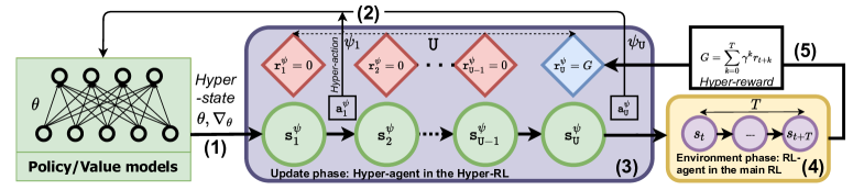
Figure 1: Hyper-RL structure. The hyper-state (green circle) is captured from the PG models’ parameters and gradients at every Hyper-RL step (1). Given the hyper-states, the hyper-agent takes hyper-actions, choosing hyperparameters for the PG method to update the models (2). The update lasts $\mathtt{U}$ steps. After the last update step (3), the RL agent starts environment phase with the current policy, collecting an empirical return $G$ after $T$ environment steps (4). $G$ is used as the hyper-reward for the last policy update step (blue diamond) (5). Other update steps (red diamond) are assigned with hyper-reward $0$.

This problem of formulating methods that can take the training context into consideration and using them as episodic experiences in optimizing hyperparameters remains unsolved. The first challenge is to effectively represent the training context of PG algorithms that often involve a large number of neural network parameters. The second challenge is sample-efficiency. Current performant hyperparameter searches (Jaderberg et al. 2017; Parker-Holder, Nguyen, and Roberts 2020) often necessitate parallel interactions with the environments, which is expensive and not always feasible in real-world applications. Ideally, hyperparameter search methods should not ask for additional observations that the PG algorithms already collect. If so, it must be solved as efficiently as possible to allow efficient training of PG algorithms.

We address both these issues with a novel solution, namely Episodic Policy Gradient Training (EPGT)–a PG training scheme that allows on-the-fly hyperparameter optimization based on episodic experiences. The idea is to formulate hyperparameter scheduling as a Markov Decision Process (MDP), dubbed as Hyper-RL. In the Hyper-RL, an agent (hyper-agent) acts to optimize hyperparameters for the PG algorithms that optimize the policy for the agent of the main RL (RL-agent). The two agents operate alternately: the hyper-agent acts to reconfigure the PG algorithms with different hyperparameters, which ultimately changes the policy of the RL agent (update phase); the RL agent then acts to collect returns (environment phase), which serves as the rewards for the hyper-agent. To build the Hyper-RL, we propose mechanisms to model its state, action and reward. In particular, we model the training context as the state of the Hyper-RL by using neural networks to compress the parameters and gradients of PG models (policy/value networks) into low-dimensional state vectors. The action in the Hyper-RL corresponds to the choice of hyperparameters and the reward is derived from the RL agent’s reward.

We propose to solve the Hyper-RL through episodic memory. As an episodic memory provides a direct binding from experiences (state-action) to final outcome (return), it enables fast utilization of past experiences and accelerates the searching of near-optimal policy (Lengyel and Dayan 2008). Unlike other memory forms augmenting RL agents with stronger working memory to cope with partial observations (Hung et al. 2019; Le, Tran, and Venkatesh 2020) or contextual changes within an episode (Le and Venkatesh 2020), episodic memory persists across agent lifetime to maintain a global value estimation. In our case, the memory estimates the value of a state-action pair in the Hyper-RL by nearest neighbor memory lookup (Pritzel et al. 2017). To store learning experience, we use a novel weighted average nearest neighbor writing rule that quickly propagates the value inside the memory by updating multiple memory slots per memory write. Our episodic memory is designed to cope with noisy and sparse rewards in the Hyper-RL.

Our key contribution is to provide a new formulation for online hyperparameter search leveraging context of previous training experiences, and demonstrate that episodic memory is a feasible way to solve this. This is also the first time episodic memory is designed for hyperparameter optimization. Our rich set of experiments shows that EPGT works well with various PG methods and diverse hyperparameter types, achieving higher rewards without significant increase in computing resources. Our solution has desirable properties, it is (i) computationally cheap and run once without parallel computation, (ii) flexible to handle many hyperparameters and PG methods, and (iii) shows consistent/significant performance gains across environments and PG methods.

Methods

Hyperparameter Reinforcement Learning (Hyper-RL)

In this paper, we address the problem of online hyperparameter search. We argue that in order to choose good values, hyperparameter search (HS) methods should be aware of the past training states. This intuition suggests that we should treat the HS problem as a standard MDP. Put in the context of HS for RL, our HS algorithm becomes a Hyper-RL algorithm besides the main RL algorithm. In Hyper-RL, the hyper-agent makes decisions at each policy update step to configure the PG algorithm with suitable hyperparameters $\psi$. The ultimate goal of the Hyper-RL is the same as the main RL’s: to maximize the return of the RL agent.

To construct the Hyper-RL, we define its state $\mathtt{s^{\psi}}$, action $\mathtt{a}^{\psi}$ and reward $\mathtt{r^{\psi}}$. Hereafter, we refer to them as hyper-state, hyper-action and hyper-reward to avoid confusion with the main RL’s $s$, $a$ and $r$. Fig. 1 illustrates the operation of Hyper-RL. In the update phase, the Hyper-RL runs for $\mathtt{U}$ steps. At each step, taking the hyper-state captured from the PG models’ parameters and gradients, the hyper-agent outputs hyper-actions, producing hyperparameters for PG algorithms to update the policy/value networks accordingly. After the last update (blue diamond), the resulting policy will be used by the RL agent to perform the environment phase, collecting returns after $T$ environment interactions. The returns will be used in the PG methods, and utilized as hyper-reward for the last policy update step. Below we detail the hyper-action, hyper-reward and hyper-state.

Hyper-action A hyper-action $\mathtt{a}^{\psi}$ defines the values for the hyperparameters $\psi$ of interest. For simplicity, we assume the hyper-action is discrete by quantizing the range of each hyperparameter into $\mathtt{B}$ discrete values. A hyper-action $\mathtt{a^{\psi}}$ selects a set of discrete values, each of which is assigned to a hyperparameter (see more Appendix A.2).

Hyper-reward The hyper-reward $\mathtt{r}^{\psi}$ is computed based on the empirical return that the RL agent collects in the environment phase after hyperparameters are selected and used to update the policy. The return is $G=\mathbb{E}_{s_{t:t+T},a_{t:t+T}}\left[\sum_{k=0}^{T}\gamma^{k}r_{t+k}\right]$ where $t$ and $T$ are the environment step and learning horizon, respectively. Since there can be $\mathtt{\mathtt{U}}$ consecutive policy update steps in the update phase, the last update step in the update phase receives hyper-reward $G$ while others get zero hyper-reward, making the Hyper-RL, in general, a sparse reward problem. That is,

$$\mathtt{r}_{i}^{\psi}=\begin{cases}G&\textrm{if }i=\mathtt{U}\\ 0&\textrm{otherwise}\end{cases}$$ (1)

To define the objective for the Hyper-RL, we treat the update phase as a learning episode. Each learning episode can lasts for multiple of $\mathtt{U}$ update steps and for each step $i$ in the episode, we aim to maximize the hyper-return $\mathtt{G}_{i}^{\psi}=\sum_{j\geq i}^{\mathtt{U}n}\mathtt{r}_{j}^{\psi}$ where $n\in\mathbb{N}^{+}$. In this paper, $n$ is simply set to 1 and thus, $\mathtt{G}_{i}^{\psi}=G$.

Hyper-state A hyper-state $\mathtt{s^{\psi}}$ should capture the current training state, which may include the status of the trained model, the loss function or the amount of parameter update. We fully capture $\mathtt{s^{\psi}}$ if we know exactly the loss surface and the current value of the optimized parameters, which can result in perfect hyperparameter choices. This, however, is infeasible in practice, thus we only model observable features of the hyper-state space. The Hyper-RL is then partially observable and noisy. In the following, we propose a method to represent the hyper-state efficiently.

0:  A parametric policy function $\pi_{\theta}$ of the main RL algorithm $PG_{\psi}(\pi_{\theta},G)$ where $\psi$ is the set of hyperparamters for training $\pi_{\theta}$ and $G$ the empirical return collected by function $Agent(\pi_{\theta})$.

1:  Initialize the episodic memory $\mathtt{M}=\emptyset$

2:  for $episode=1,2,...$ do {loop over learning episodes}

3:     Initialize a buffer $\mathtt{D}=\emptyset${storing hyper-state, action, and reward within a learning episode}

4:     for $i=1,\dots\mathtt{U}$ do {loop over policy updates}

5:        Compute $\phi(\mathtt{s}^{\psi}_{i})$. Select $\mathtt{a}^{\psi}_{i}$ by $\epsilon$-greedy with $\mathtt{Q}\left(\mathtt{s}_{i}^{\psi},\mathtt{a}^{\psi}\right)=\mathtt{M.read}\left(\phi\left(\mathtt{s}^{\psi}_{i}\right),\mathtt{a}^{\psi}\right)$ (Eq. Episodic Control for solving the Hyper-RL)

6:        Convert $\mathtt{a}^{\psi}_{i}$ to the hyperparameter values $\psi_{i}$ and update $\theta\leftarrow PG_{\psi_{i}}(\pi_{\theta},G)$

7:        Compute $\mathtt{r}^{\psi}_{i}$ (Eq. 1). Add $(\phi(\mathtt{s}^{\psi}_{i}),\mathtt{a}^{\psi}_{i},\mathtt{r}^{\psi}_{i})$ to $\mathtt{D}$

8:        $\mathbf{if}$ $i$ == $\mathtt{U}$ $\mathbf{then}$ $G=Agent(\pi_{\theta})$

9:     end for

10:     Update episodic memory with $\mathtt{M.update(D)}$ (Eq. 4)

11:  end for

Algorithm 1 Episodic Policy Gradient Training.

Hyper-state representation Our hypothesis is that one signature feature of the hyper-state is the current value of optimized parameters $\theta$ and the derivatives of the PG method’s objective function w.r.t $\theta$. We maintain a list of the last $N_{order}$ first-order derivatives: $\left\{\nabla_{\theta n}\right\}_{n=1}^{N_{order}}$, which preserves information of high-order derivatives (e.g. a second-order derivative can be estimated by the difference between two consecutive first-order derivatives). Let us denote the parameters and their derivatives, often in tensor form, as $\theta=\left\{W_{m}^{0}\right\}_{m=1}^{M}$ and $\nabla_{\theta n}=\left\{W_{m}^{n}\right\}_{m=1}^{M}$ where $M$ is the number of layers in the policy/value network. $\left\{\theta,\nabla_{\theta n}\right\}$ can be denoted jointly $\left\{W_{m}^{n}\right\}_{n=0,m=1}^{N_{order},M}$ or $\left\{W_{m}^{n}\right\}$ for short (see Appendix B.4 for dimension details of $W_{m}^{n}$).

Merely using $\left\{W_{m}^{n}\right\}$ to represent the learning state is still challenging since the number of parameters is enormous as it often is in the case of recent PG methods. To make the hyper-state tractable, we propose to use linear transformation to map the tensors to lower-dimensional features and concatenate them to create the state vector $\mathtt{s^{\psi}}=\left[s_{m}^{n}\right]_{n=0,m=1}^{N_{order},M}$. Here, $s_{m}^{n}$ is the feature of $W_{m}^{n}$, computed as

$$s_{m}^{n}=\mathtt{vec}\left(W_{m}^{n}C_{m}^{n}\right)$$ (2)

where $C_{m}^{n}\in\mathbb{R}^{d^{nm}\text{$\times d$}}$ is the transformation matrix, $d^{nm}$ the last dimension of $W_{m}^{n}$ ($d^{nm}\gg d$) and $\mathtt{vec}\left(\cdot\right)$ the vectorize operator, flattening the input tensor. To make our representation robust, we propose to learn the transformation $C_{m}^{n}$ as described in the next section.

Learning to represent hyper-state and memory key We map $\mathtt{s^{\psi}}$ to its embedding by using a feed-forward neural network $\phi$, resulting in the state embedding $\phi\left(\mathtt{s^{\psi}}\right)\in\mathbb{R}^{h}$. $\phi\left(\mathtt{s}^{\psi}\right)$ later will be stored as the key of the episodic memory. We can just use random $\phi$ and $C_{m}^{n}$ for simplicity. However, to encourage $\phi\left(\mathtt{s}^{\psi}\right)$ to store meaningful information of $\mathtt{s}^{\psi}$, we propose to reconstruct $\mathtt{s}^{\psi}$ from $\phi\left(\mathtt{s}^{\psi}\right)$ via another decoder network $\omega$ and minimize the following reconstruction error $\mathcal{L}_{rec}=\left\|\omega\left(\phi\left(\mathtt{s^{\psi}}\right)\right)-\mathtt{s^{\psi}}\right\|_{2}^{2}$. Similar to (Blundell et al. 2016), we employ latent-variable probabilistic models such as VAE to learn $C_{m}^{n}$ and update the encoder-decoder networks. Thanks to using $C_{m}^{n}$ projection to lower dimensional space, the hyper-state distribution becomes simpler and potential for VAE reconstruction. Notably, the VAE is jointly trained online with the RL agent and the episodic memory (more details in Appendix A.3).

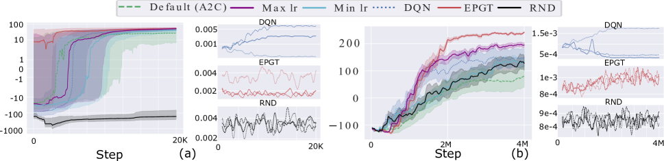
Figure 2: Performance on (a) MountainCarContinuous (log scale) and (b) BipedalWalker over env. steps. In each plot, average return is on the left with mean and std. over 10 runs. The right is smoothed (taking average over a window of 100 steps) learning rate $\alpha$ found by the baselines (first 3 runs).

Episodic Control for solving the Hyper-RL

Theoretically, given the hyper-state, hyper-action and hyper-reward clearly defined in the previous section, we can use any RL algorithm to solve the Hyper-RL problem. However, in practice, the hyper-reward is usually sparse and the number of steps of the Hyper-RL is usually much smaller than that of the main RL algorithm ($\text{$\mathtt{U}$}\ll T$). It means parametric methods (e.g. DQN) which require a huge number of update steps are not suitable for learning a good approximation of the Hyper-RL’s Q-value function $\mathtt{Q}\left(\mathtt{s}_{i}^{\psi},\mathtt{a}_{i}^{\psi}\right)$.

To quickly estimate $\mathtt{Q}\left(\mathtt{s}_{i}^{\psi},\mathtt{a}_{i}^{\psi}\right)$, we maintain an episodic memory that lasts across learning episodes and stores the outcomes of selecting hyperparameters from a given hyper-state. We hypothesize that the training process involves hyper-states that share similarities, which is suitable for episodic recall using KNN memory lookup. Concretely, the episodic memory $\mathtt{M}$ binds the learning experience $\left(\phi\left(\mathtt{s}_{i}^{\psi}\right),\mathtt{a}_{i}^{\psi}\right)$–the key, where $\phi$ is an embedding function, to the approximated expected hyper-return $\mathtt{\tilde{G}}_{i}^{\psi}$–the value. We index the memory using key $\left(\phi\mathtt{\left(\mathtt{s}_{i}^{\psi}\right)},\mathtt{a}_{i}^{\psi}\right)$ to access the value, a.k.a $\mathtt{M}\left[\phi\mathtt{\left(\mathtt{s}_{i}^{\psi}\right)},\mathtt{a}_{i}^{\psi}\right]=\mathtt{\tilde{G}}_{i}^{\psi}$. Computing and updating the $\mathtt{Q}\left(\mathtt{\mathtt{s}_{i}^{\psi}},\mathtt{a}_{i}^{\psi}\right)$ corresponds to two memory operators: $\mathtt{read}$ and $\mathtt{update}$. The $\mathtt{read}\left(\phi\left(\mathtt{s}_{i}^{\psi}\right),\mathtt{a}_{i}^{\psi}\right)$ takes the hyper-state embedding plus hyper-action and returns the hyper-state-action value $\mathtt{Q}\left(\mathtt{s}_{i}^{\psi},\mathtt{a}_{i}^{\psi}\right)$. The $\mathtt{update}\left(\mathtt{D}\right)$ takes a buffer $\mathtt{D}$ containing observations $(\mathtt{s}_{i}^{\psi},\mathtt{a}_{i}^{\psi},\mathtt{r}_{i}^{\psi})_{i=1}^{\mathtt{U}}$, and updates the content of the memory $\mathtt{M}$. The details of the two operators are as follows.

Memory reading Similarly to (Pritzel et al. 2017), we estimate the state-action value of any $\mathtt{s}_{i}^{\psi}$-$\mathtt{a}_{i}^{\psi}$ pair by:

$$\mathtt{Q}\left(\mathtt{s}_{i}^{\psi},\mathtt{a}_{i}^{\psi}\right) = \mathtt{\mathtt{read}}\left(\mathtt{s}_{i}^{\psi},\mathtt{a}_{i}^{\psi}\right)$$

$$= \frac{\sum_{k=1}^{|\mathcal{N}(i)|}Sim\left(i,k\right)\mathtt{M}\left[\phi\left(\mathtt{s}_{k}^{\psi}\right),\mathtt{a}_{i}^{\psi}\right]}{\sum_{k=1}^{|\mathcal{N}(i)|}Sim\left(i,k\right)}$$

where $\mathcal{N}(i)$ denotes the neighbor set of the embedding $\phi\left(\mathtt{s}_{i}^{\psi}\right)$ in $\mathtt{M}$ and $\phi\left(\mathtt{s}_{k}^{\psi}\right)$ the $k$-th nearest neighbor. $\mathcal{N}(i)$ includes $\phi\left(\mathtt{s}_{i}^{\psi}\right)$ if it exists in $\mathtt{M}$. $Sim\left(i,k\right)$ is a kernel measuring the similarity between $\phi\left(\mathtt{s}_{k}^{\psi}\right)$ and $\phi\left(\mathtt{s}_{i}^{\psi}\right)$.

Memory update To cope with noisy observations from the Hyper-RL, we propose to use weighted average to write the hyper-return to the memory slots. Unlike max writing rule (Blundell et al. 2016) that always stores the best return, our writing propagates the average return inside the memory, which helps cancel out the noise of the Hyper-RL. In particular, for each observed transition in a learning episode (stored in the buffer $\mathtt{D}$), we compute the hyper-return $\mathtt{G}_{i}^{\psi}$. The hyper-return is then used to update the memory such that the action value of $\phi\left(\mathtt{s}_{i}^{\psi}\right)$’s neighbors is adjusted towards $\mathtt{G}_{i}^{\psi}$ with speeds relative to the distances (Le et al. 2021):

$$\mathtt{M}\left[\phi\left(\mathtt{s}_{k}^{\psi}\right),\mathtt{a}_{i}^{\psi}\right] \leftarrow\mathtt{M}\left[\phi\left(\mathtt{s}_{k}^{\psi}\right),\mathtt{a}_{i}^{\psi}\right]+\beta\frac{\Delta_{ik}Sim\left(i,k\right)}{\sum_{k=1}^{|\mathcal{N}(i)|}Sim\left(i,k\right)}$$ (4)

where $\phi\left(\mathtt{s}_{k}^{\psi}\right)$ is the $k$-th nearest neighbor of $\phi\left(\mathtt{s}_{i}^{\psi}\right)$ in $\mathcal{N}(i)$, $\Delta_{ik}=\mathtt{G}_{i}^{\psi}-\mathtt{M}\left[\phi\left(\mathtt{s}_{k}^{\psi}\right),\mathtt{a}_{i}^{\psi}\right]$, and $0<\beta<1$ the writing rate. If the key $\left(\phi\left(\mathtt{s}_{i}^{\psi}\right),\mathtt{a}_{i}^{\psi}\right)$ is not in $\mathtt{M}$, we also add $\left(\phi\left(\mathtt{s}_{i}^{\psi}\right),\mathtt{a}_{i}^{\psi},\mathtt{G}_{i}^{\psi}\right)$ to the memory. When the stored tuples exceed memory capacity $N_{mem}$, the earliest added tuple will be removed.

Under this formulation, $\mathtt{M}\left[\phi\left(\mathtt{s}_{i}^{\psi}\right),\mathtt{a}_{i}^{\psi}\right]$ is an approximation of the expected hyper-return collected by taking the hyper-action $\mathtt{a}_{i}^{\psi}$ at the hyper-state $\mathtt{s}_{i}^{\psi}$ (see Appendix C for proof). As we update several neighbors at one write, the hyper-return propagation inside the episodic memory is faster and helps to handle the sparsity of the Hyper-RL. Unless stated otherwise, we use the same neighbor size $|\mathcal{N}(i)|$ for both reading and writing process, denoted as $K$ for short.

Integration with PG methods Our episodic control mechanisms can be used to estimate the hyper-state-action-value of the Hyper-RL. The hyper-agent uses that value to select the hyper-action through $\epsilon$-greedy policy and schedule the hyperparameters of PG methods. Algo. 1, Episodic Policy Gradient Training (EPGT), depicts the use of our episodic control with a generic PG method.

Experimental results

Across experiments, we examine EPGT with different PG methods including A2C (Mnih et al. 2016), ACKTR (Wu et al. 2017) and PPO (Schulman et al. 2017). We benchmark EPGT against the original PG methods with tuned hyperparameters and 4 recent hyperparameter search methods. The experimental details can be found in the Appendix B.

Why episodic control?

In this section, we validate the choice of episodic control to solve the proposed Hyper-RL problem. As such, we choose A2C as the PG method and examine EPGT, random hyper-action (RND) and DQN (Mnih et al. 2015) as 3 methods to schedule the learning rate ($\alpha$) for A2C. We also compare with A2C using different fixed-$\alpha$ within the search range (default, min and max learning rates). We test on 2 environments: Mountain Car Continuous (MCC) and Bipedal Walker (BW) with long and short learning rate search ranges ($[4\times 10^{-5},10^{-2}]$ and $[2.8\times 10^{-4},1.8\times 10^{-3}]$, respectively).

Fig. 2 demonstrates the learning curves and learning rate schedules found by EPGT, RND and DQN. In MCC, the search range is long, which makes RND performance unstable, far lower than the fixed-$\alpha$ A2Cs. DQN also struggles to learn good $\alpha$ schedule for A2C since the number of trained environment steps is only 20,000, which corresponds to only 4,000 steps in the Hyper-RL. This might not be enough to train DQN’s value network and leads to slower learning. On the contrary, EPGT helps A2C achieve the best performance faster than any other baseline. In BW, thanks to shorter search range and large number of training steps, RND and DQN show better results, yet still underperform the best fixed-$\alpha$ A2C. By contrast, EPGT outperforms the best fixed-$\alpha$ A2C by a significant margin, which confirms the benefit of episodic dynamic hyperparameter scheduling.

Besides performance plots, we visualize the selected values of learning rates over training steps for the first 3 runs of each baseline. Interestingly, DQN finds more consistent values, often converging to extreme learning rates, indicating that the DQN mostly selects the same action for any state, which is unreasonable. EPGT, on the other hand, prefers moderate learning rates, which keep changing depending on the state. Compared to random schedules by RND, those found by EPGT have a pattern, either gradually decreasing (MCC) or increasing (BW). In terms of running time, EPGT runs slightly slower than A2C without any scheduler, yet much faster than DQN (see Appendix’s Table 5).

Model	HalfCheetah	Hopper	Ant	Walker
TMG♠	1,568	378	950	492
HOOF♠	1,523	350	952	467
HOOF♢	1,427±293	452±40.7	954±8.57	674±195
EPGT	2,530±1268	603±187	1,083±126	888±425

Table 1: EPGT vs sequential online hyperparameter search (A2C as the PG). Bold denotes statistically better results in terms of Cohen effect size $>0.5$. We train agents for 5 million steps and report the mean (and std. if applicable) over 10 runs. $\spadesuit$ is from (Paul, Kurin, and Whiteson 2019) (no std. reported) and $\diamondsuit$ is our run.

Model	BW	LLC	Hopper	IDP
PBT${}^{\text{\textdegree}}$	223	159	1492	8,893
PB2${}^{\text{\textdegree}}$	276	235	2,346	8,893
PB2♢	280	223	2,156	9,253
EPGT	282	235	3,253	9,322

Table 2: EPGT vs parallel online hyperparameter search (PPO as the PG). Following (Parker-Holder, Nguyen, and Roberts 2020), we train the PPO agents for 1 million steps and report the best median over 10 runs.° denotes the numbers reported in (Parker-Holder, Nguyen, and Roberts 2020), and $\diamondsuit$ is our run.

EPGT vs online hyperparameter search methods

Our main baselines are existing methods for dynamic tuning of hyperparameters of policy gradient algorithms, which can be divided into 2 groups: (i) sequential HOOF (Paul, Kurin, and Whiteson 2019) and Meta-gradient (Xu, van Hasselt, and Silver 2018) and (ii) parallel PBT (Jaderberg et al. 2017) and PB2 (Parker-Holder, Nguyen, and Roberts 2020). We follow the same experimental setting (PG configuration and environment version) and apply our EPGT to the same set of optimized hyperparameters, keeping other hyperparameters as in other baselines. We also rerun the baselines HOOF and PB2 using our codebase to ensure fair comparison. For the first group, the PG method is A2C and only the learning rate is optimized, while for the second group, the PG method is PPO and we optimize 4 hyperparameters (learning rate $\alpha$, batch size $b$, GAE $\lambda$ and PPO clip $\epsilon$).

Table 1 reports the mean test performance of EPGT against Tuned Meta-gradient (TMG) and HOOF on 4 Mujoco environments. EPGT demonstrates better results in all 4 tasks where HalfCheetah, Hopper and Walker observe significant gain. Notably, compared to HOOF, EPGT exhibits higher mean and variance, indicating that EPGT can find distinctive solutions, breaking the local optimum bottleneck of other baselines.

Table 2 compares EPGT with PBT and PB2 on corresponding environments and evaluation metrics. In the four tasks used in PB2 paper, EPGT achieves better median best score for 3 tasks while maintaining competitive performance in LLC task. We note that EPGT is jointly trained with the PG methods in a single run and thus, achieves this excellent performance without parallel interactions with the environments as PB2 or PBT. Learning curves of our runs for the above tasks are in Appendix B.3.

EPGT vs grid-search/manual tuning

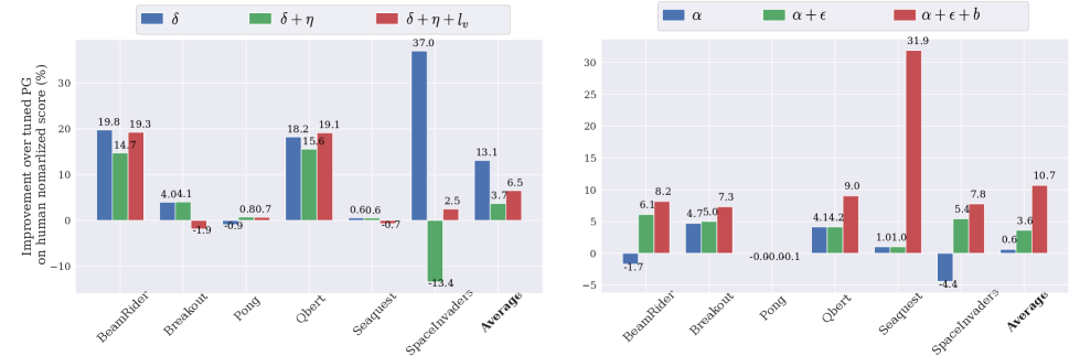
Figure 9: Atari games: Average return over environment steps across 5 training seeds using PG ACKTR (left) amd PPO (right).

Atari We now examine EPGT on incremental sets of hyperparameters. We adopt 6 standard Atari games and train 2 PG methods: ACKTR and PPO for 20 million steps per game. For ACKTR, we apply EPGT to schedule the trust region radius $\delta$, step size $\eta$ and the value loss coefficient $l_{v}$. For PPO, the optimized hyperparameters are learning rate $\alpha$, trust region clip $\epsilon$ and batch size $b$. These are important and already tuned hyperparameters for Atari task by prior works. We form 3 hyperparameter sets for each PG method. For each set, we further perform grid search near the default hyperparameters and record the best tuned results. We compare these results with EPGT’s and report the relative improvement on human normalized score (see Fig. 3 for the case of ACKTR, full in Appendix Fig. 9).

The results indicate that, for all hyperparameter sets, EPGT on average show gains up to more than 10% over tuned PG methods. For certain games, the performance gain can be more than 30%. Jointly optimizing more hyperparameters is generally better for PPO while optimizing only $\delta$ gets the most improvement for ACKTR.

Mujoco Here, we conduct experiments on 6 Mujoco environments: HalfCheetah, Hooper, Walker2d, Swimmer, Ant and Humanoid. For the last two challenging tasks, we train with 10M steps while the others 1M steps. The set of optimized hyperparameters are $\left\{\alpha,\epsilon,\lambda,b\right\}$. The baseline Default (PPO) has fixed hyperparameters, which are well-tuned by previous works, and PB2 uses the same hyperparameter search range as our method. Random hyper-action (RND) baseline is included to see the difference between random and episodic policy in Hyper-RL formulation.

On 6 Mujoco tasks, on average, EPGT helps PPO earn more than 583 score while PB2 fails to clearly outperform the tuned PPO (see more in Appendix Fig. 12). Fig. 4 (left) illustrates the result on HalfCheetah where performance gap between EPGT and other baselines can be clearly seen. Despite using the same search range, PB2 and RND show lower average return. We include the hyperparameters used by EPGT and RND throughout training in Fig. 4 (right). Overall, EPGT’s schedules do not diverge much from the default values, which are already well-tuned. However, we can see a pattern of using smaller hyperparameters during middle phase of training, which aligns with the moments when there are changes in the performance.

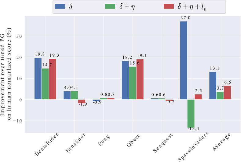
Figure 3: Performance improvement on 6 Atari games applying EPGT to optimize incremental sets of hyperparameters with ACKTR as PG. We run each game for 20 million frames and report the average over 5 runs.

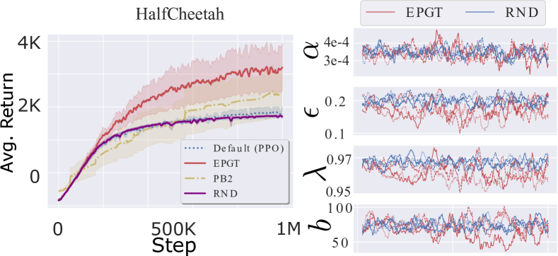
Figure 4: Performance on the representative HalfCheetah task over env. steps. The left is testing return over training iterations (mean $\pm$ std. over 10 runs) and the right hyperparameters schedule for PG methods found by EPGT and RND in the first 3 runs.

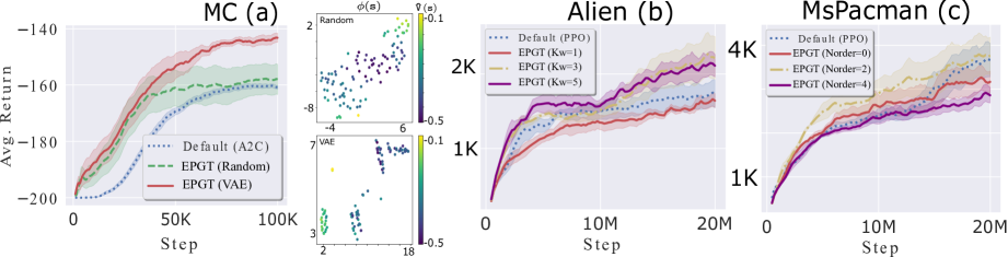
Figure 5: (a) Performance (left) and hyper-state representations $\phi\left(\mathtt{s}^{\psi}\right)$ (right) on Mountain Car (MC) using PG A2C where t-SNE is used to project $\phi\left(\mathtt{s}^{\psi}\right)$ to 2d space, showing the quality of representation learned by VAE (below) versus Random mapping (above). Performance on Alien (b) and MsPacman (c) using PG PPO with different $K_{w}$ and $N_{order}$, respectively. The curves are mean and std. over 5 runs.

Ablation studies

In this section, we describe the hyperparameter selection for EPGT used in above the experiments. We note that although EPGT introduces several hyperparameters, it is efficient to pick reasonable values and keep using them across tasks.

Learning to represent the hyper-state The hyper-state is captured by projecting the model’s weights and their gradients to a low-dimensional vectors using $C_{m}^{n}$. The state is further transformed to the memory’s key using the mapping network $\phi$. Here, we validate the choice of using VAE to learn $C_{m}^{n}$ and $\phi$ by comparing it with random mapping. We use PG A2C and test the two EPGT variants on Mountain Car (MC). Fig. 5 (a, left) demonstrates that EPGT with VAE training learns fastest and achieves the best convergence. EPGT with random projections can learn fast but shows similar convergence as the original A2C.

We visualize the final representations $\phi\left(\mathtt{s}^{\psi}\right)$ by using t-SNE and use colors to denote the corresponding average values $\mathtt{\hat{V}\left(\mathtt{s}^{\psi}\right)}=\sum_{a}\mathtt{M\left(\phi\left(\mathtt{s^{\psi}}\right),a^{\psi}\right)}$ in Fig. 5 (a, right). The upper figure is randomly projected hyper-states and the lower VAE-trained ones at 5,000 environment step. From both figures, we can see that similar-value states tend to lie together, which validates the hypothesis on existing similar training contexts. Compared to the random ones, the representations learned by VAE exhibit clearer clusters. Cluster separation is critical for nearest neighbor memory access in episodic control, and thus explains why VAE-trained EPGT outperforms random EPGT significantly. Notably, training the VAE is inexpensive. Empirical results demonstrates that with reasonable hyper-state sizes, the VAE converges quickly (see Appendix Fig. 6).

Writing rule To verify the contribution of our proposed writing rule, we test different number of writing neighbor size ($K_{w}$). In this experiment, the reading size is fixed to 3 and different from the writing size. Fig. 5 (b) shows the learning curves of EPGT using different $K_{w}$ against the original PPO. When $K_{w}=1$, our rule becomes single-slot writing as in (Blundell et al. 2016; Pritzel et al. 2017), which even underperforms using default hyperparameters. By contrast, increasing $K_{w}=3$ boosts EPGT’s performance dramatically, on average improving PPO by around 500 score in Alien game. Increasing $K_{w}$ further seems not helpful since it may create noise in writing. Thus, we use $K_{w}=3$ in all of our experiments. Others showing our average writing rule is better than traditional max rule and examining different numbers of general neighbor size $K$ are in Appendix B.4.

Order of representation Finally, we examine EPGT’s performance with different order of representation ($N_{order}$). $N_{order}=0$ means the hyper-state only includes the parameters $\theta$. Increasing $N_{order}$ gives more information, providing better state representations. That holds true in MsPacman game when we increase the order from $0$ to $2$ as shown in Fig. 5 (c). However, when $N_{order}$ is set to 4, the performance drops since the hyper-states now are in a very high dimension ($16K$) and VAE does not work well in this case. Hence, we use $N_{order}=2$ for all of our experiments.

Related works

Hyperparameter search Automatic hyperparameter tuning generally requires multiple training runs. Parallel search methods such as grid or random search (Bergstra and Bengio 2012; Larochelle et al. 2007) perform multiple runs concurrently and pick the hyperparameters that achieve best result. These methods are simple yet expensive. Sequential search approaches reduce the number of runs by consecutively executing experiments using a set of candidate hyperparameters and utilize the evaluation result to guide the subsequent choice of candidates (Hutter, Hoos, and Leyton-Brown 2011). Bayesian Optimization approaches (Brochu, Cora, and De Freitas 2010) exploit the previous experimental results to update the posterior of a Bayesian model of hyperparameters and explore promising hyperparameter regions. They have been widely used in hyperparameter tuning for various machine learning algorithms including deep learning (Snoek, Larochelle, and Adams 2012; Klein et al. 2017). Recently, to speed up the process, distributed versions of BO are also introduced to evaluate in parallel batches of hyperparameter settings (González et al. 2016; Chen et al. 2018).

However, these approaches still suffer from the issue of computational inefficiency, demanding high computing resources, increasing the training time significantly. If applied to RL, they require more environment interactions, which leads to sample inefficiency. In addition, the hyperparameters found by these methods are usually fixed, which can be suboptimal (Luketina et al. 2016). Inspired by biological evolution, population-based methods initially start as random search then select best performing hyperparameter instances to generate subsequent hyperparameter candidates, providing a hybrid solution between parallel and sequential search (Fiszelew et al. 2007; Young et al. 2015).

Recent works propose using evolutionary algorithms to jointly learn the weights and hyperparameters of neural networks under supervised training (Jaderberg et al. 2017; Li et al. 2019). In BPT (Jaderberg et al. 2017) as an example, multiple training are executed asynchronously and evaluated periodically. Under-performing models are replaced by better ones whose hyperparameters evolve to explore better configurations. This approach allows hyperparameter scheduling on-the-fly but still requires a large number of parallel runs and are thus unsuitable for machines with small computational budget.

On-the-fly hyperparameter search for reinforcement learning Early works on gradient-based hyperparameter search focus on learning rate adjustment (Sutton 1992; Bengio 2000). The approach has been recently extended to RL by using the meta-gradient of the return function to adjust the hyperparameters such as discount factor or bootstrapping parameter (Xu, van Hasselt, and Silver 2018). Hence, in this approach, the return needs to be a differentiable function w.r.t the hyperparameters, which cannot extend to any hyperparameter type such as “clip” or policy gradient algorithm such as TRPO.

HOOF (Paul, Kurin, and Whiteson 2019) is an alternative to meta-gradient methods wherein hyperparameter optimization is done via random search and weighted important sampling. The method relies on off-policy estimate of the value of the policy, which is known to have high variance and thus requires enforcing additional KL constraint. The search is also limited to some specific hyperparameters. Population-based approaches have been applied to RL hyperparameter search. These methods become more efficient by utilizing off-policy PG’s samples (Tang and Choromanski 2020) and small-size population (Parker-Holder, Nguyen, and Roberts 2020), showing better results than PBT or BO in RL domains. However, they still suffer from the inherited expensive computation issue of population-based training. All of these prior works do not formulate hyperparameter search as a MDP, bypassing the context of training, which is addressed in this paper.

Discussion

We introduced Episodic Policy Gradient Training (EPGT), a new approach for online hyperparameter search using episodic memory. Unlike prior works, EPGT formulates the problem as a Hyper-RL and focuses on modeling the training state to utilize episodic experiences. Then, an episodic control with improved writing mechanisms is employed to search for optimal hyperparameters on-the-fly. Our experiments demonstrate that EPGT can augment various PG algorithms to optimize different types of hyperparameters, achieving better results. Current limitations of EPGT are the coarse discrete action spaces and simplified hyper-state modeling using linear mapping. We will address these issues and extend our approach to supervised training in future works.

ACKNOWLEDGMENTS

This research was partially funded by the Australian Government through the Australian Research Council (ARC). Prof Venkatesh is the recipient of an ARC Australian Laureate Fellowship (FL170100006).

Appendix

A. Details of methodology

A.1 Hyper-reward design

Each step of the Hyper-RL requires a hyper-reward. The hyper-reward reflects how well the hyper-agent is performing to help the RL agent in the main RL’s environment. The tricky part is the RL agent’s performance is not always measured at every Hyper-RL step (policy update step).

We define $\mathtt{U}$ the interval of Hyper-RL steps (the update phase) between 2 performance measurement of the RL agent. At the end of each update phase, after taking hyper-action and update models, the performance is evaluated in the environment phase, resulting in the roll-out return $G$, which will be used as hyper-reward for the final step of the update phase. For in-between steps in the update phase, there is no direct way to know the intermediate outcome of each hyper-action, hence a hyper-reward $0$ is assigned, making Hyper-RL generally a sparse problem.

One may think of assigning in-between steps the same hyper-return, which is collected from the previous/next environment phase to avoid sparse hyper-reward. However, it does not make sense to use past/future outcomes to assign reward for current steps. Hence, we choose the sparse reward scheme and that is also one motivation for using episodic memory.

Since EPGT reuses PG return, it does not require extra computation for hyper-reward, unlike HOOF (recomputing returns with important sampling) or population-based methods (collecting return in parallel).

A.2 Hyper-action quantization

For most types of hyperparameters, we use uniform quantization within a range around the default value to derive the hyper-action. For example, when $\mathtt{B}=3$, GAE’s $\lambda$ will have the possible values $\left\{0.95,0.975,0.99\right\}$ and PPO’s clip $\epsilon\in$ $\left\{0.1,0.2,0.3\right\}$

For learning rate, uniform quantization for a certain range will not necessarily include the default learning rate, which can be a good candidate for the hyperparameter. Hence, we use a different quantization formula as follows,

$$\left\{\frac{\alpha^{*}}{\left(\mathtt{B}-1\right)/2},...,\frac{\alpha^{*}}{2},\alpha^{*},\alpha^{*}\times 2,...,\alpha^{*}\times\left(B-1\right)/2\right\}$$ (5)

where $\alpha^{*}$ is the default learning rate (for A2C, e.g. $\alpha^{*}=7\times 10^{-4}$). This is convenient for automatically generating the bins for hyper-action space given $\mathtt{B}$, which ensures that there exists one action that correspond to the default hyperparameter.

One limitation of discretizing hyper-actions is the exponential growth of the number of hyper-action w.r.t the size of the optimized hyperparameter set. For example, if there are $\left\|\psi\right\|$ hyperparameters we want to optimize on-the-fly and each is quantized into $\mathtt{B_{i}}$ discrete values, the number of hyper-actions is

$$\mathtt{\left\|A\right\|=\mathtt{\prod_{i}^{\left\|\psi\right\|}B_{i}}}$$

In this paper, our experiments scale up to $\left\|\mathtt{A}\right\|=3\times 3\times 4\times 4=144$. Beyond this limit may require a different way to model the hyper-action space (e.g. RL methods for continuous action space).

A.3 EPGT’s networks

EPGT has trainable parameters, which are $C_{m}^{n}$, $\phi$ and $\omega$. Here, $C_{m}^{n}$ is just a parametric 2d tensor, $\phi$ and $\omega$ are neural networks, implemented as follows:

• Encoder network $\phi$: 2-layer feed-forward neural network with $\tanh$ activation with layer size: $d\rightarrow d/4\rightarrow h\times 2$. The output will be used as the mean and the standard deviation of the normal distribution in VAE.

• Decoder network $\omega$: 2-layer feed-forward neural network with $sigmoid$ activation with layer size: $h\rightarrow d/4\rightarrow d$

The number of parameters will increase as the PG networks grow. For PPO as the most complicated example, EPGT’s number of parameters is 5M.

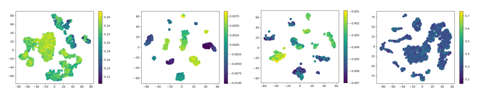
Figure 15: Hyper-state representations stored in memory for BipedalWalker, HalfCheetah, Ant, Riverraid tasks (from left to right) at 1000 update steps.

To train the networks, we sample hyper-states in the buffer $\mathtt{D}$ and minimize $\mathcal{L}_{rec}=\left\|\omega\left(\phi\left(\mathtt{s}^{\psi}\right)\right)-\mathtt{s^{\psi}}\right\|_{2}^{2}$ using gradient decent and batch size of 8. Here, we stop the gradient at the target $\mathtt{s}^{\psi}$ and only let the gradient backpropagated via $\omega\left(\phi\left(\mathtt{s^{\psi}}\right)\right)$ to learn $\omega$,$\phi$ and $\left\{C_{m}^{n}\right\}_{n=0,m=1}^{N_{order},M}$. In our experiments, to save computing cost, we do not sample every learning step. Instead, every 10 policy update steps, we sample data and perform a gradient decent step to minimize $\mathcal{L}_{rec}$ once. Training, interestingly, is usually sample-efficient, especially when $d$ is not big and PG networks are simple. Fig. 6 showcases the reconstruction loss $\mathcal{L}_{rec}$ in several environments using PG A2C and PPO. For PG A2C, convergence is quickly achieved since A2C’s network for Bipedal Walker and HalfCheetah is simple. For PPO, the task is more challenging and also the networks include CNN (in case of Atari game Riverraid). Hence, the loss is minimized slower, yet still showing good convergence. We note that the model learn meaning representations and the mapping is not degenerated. According to Fig. 5, our learned mapping distributes states to clusters, showing clear discrimination between similar and dissimilar states (see more in Fig. 15).

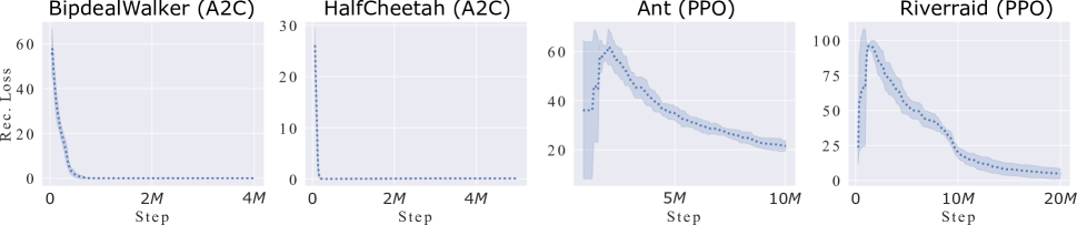
Figure 6: Reconstruction loss training VAE in representative environments and PG methods. The curves are mean with std. over 5 runs.

B. Details of experiments

B.1 A summary of tasks and PG methods

We use environments from Open AI gyms , which are public and using The MIT License. Mujoco environments use Mujoco software (our license is academic lab). Table 3 lists all the environments.

All PG methods (A2C, ACKTR, PPO) use available public code. They are Pytorch reimplementation of OpenAI’s stable baselines, which can reproduce the original performance relatively well. The source code for baselines HOOF and PB2 is adopted from the authors’ public code and , respectively. Table 4 summarizes the PG methods and their networks.

Tasks	Continuous	Gym
	action	category
Mountain Car-v0	$\mathit{\mathtt{X}}$	Classical
Mountain Car Continuous-v0	$\checked$	control
Bipedal Walker-v3	$\checked$	Box2d
Lunar Lander Continuous-v2
MuJoCo tasks (v2): HalfCheetah	$\checked$	MuJoCo
Walker2d, Hopper, Ant
Swimmer, Humanoid,
Atari games (NoFramskip-v4):	$\mathit{\mathtt{X}}$	Atari
Beamrider, Breakout, Pong
Qbert, Seaquest, SpaceInvaders
Alien, MsPacman, Demonattack
Riverraid

Table 3: Tasks used in the paper.

PGs	Policy/Value networks
A2C/ACKTR/PPO	Vector input: 2-layer feedforward
	net (tanh, h=32)
	Image input: 3-layer ReLU CNN with
	kernels $\left\{32/8/4,64/4/2,32/3/1\right\}$+2-layer
	feedforward net (ReLU, h=512)

Table 4: PG methods used in the paper.

B.2 Episodic memory configuration

We implement the memory using kd-tree structure, so neighbor lookup for memory $\mathtt{read}$ and $\mathtt{update}$ is fast. To further reduce computation complexity, we only update the memory after every 10 policy update steps. The memory itself has many hyperparameters. However, to keep our solution efficient, we keep most of the hyperparameters unchanged across experiments and do not tune them. In particular, the list of untuned hyperparameters is:

• Hyperparameters of the VAE (see A.3)

• State embedding size $h=32$

• The writing rate $\beta=0.5$

• Similarity kernel $Sim\left(i,k\right)=\frac{1}{\left\|\phi\left(\mathtt{s}_{k}^{\psi}\right)-\phi\left(\mathtt{s}_{i}^{\psi}\right)\right\|+\epsilon}$, $\epsilon=0.001$ following [31]

• $\epsilon$ in the $\epsilon$-greedy is linearly reduced from 1.0 to 0 during the training. At the final step of training, $\epsilon=0$.

• The memory size $N_{mem}$ is always half of the number of policy update steps for each task. This is determined by our educated guess that after half of training time, the initial learning experiences stored in the memory is not relevant anymore and needed to be replace with newer observations. The number of policy update steps can be always computed given the allowed number of environment steps. For example, if we allow $n_{e}$ environment steps for training, then the number of policy updates is $\frac{n_{e}\times\mathtt{U}}{T}$ , and the memory size will be $\frac{n_{e}\times\mathtt{U}}{20T}$ (since we update every 10 steps). Here, we assume each memory update will add a new tuple to the memory since the chance of exact key match is very small. For all of our tasks, the maximum $N_{mem}$ is up to 10,000.

• To hasten the training with EPGT, we utilize uniform writing [20] to reduce the compute complexity of memory writing operator. In particular, we write observations to the episodic memory every 10 update steps.

For other hyperparameters of EPGT, we tune or verify them in Mountain Car or one Atari game and apply the found hyperparameter values to all other tasks. These hyperparameters are:

• VAE or Random projection, verified in Mountain Car

• Order of representation $N_{order}$, tuned in MsPacman

• State size $d$, tuned in MsPacman

• Neighbor size $K$, tuned in Demon Attack and Alien

The details of selecting values for these hyperparameters can be found in ablation studies in this paper. We note that after verifying reasonable values for these EPGT hyperparameters in some environments, we keep using them across all experiments, and thus do not requires additional tunning per task.

B.3 Training description

All the environments are adopted from Open AI’s Gym (MIT license).

Mountain Car Continuous and Bipedal Walker with PG A2C

We use the A2C with default hyperparameters from Open AI. In these two tasks, we optimize the learning rate $\alpha$ from the range defined by Eq. 5 using $\mathtt{B}=15$ and $\mathtt{B=5}$, respectively. Here, $\mathtt{U=10}$. In this task, we implement 2 additional baselines solving the Hyper-RL: DQN and Random (RND) agent. Both DQN and RND uses the same hyper-state (trained with VAE), action and reward representation as EPGT. We note that these baselines are used to optimize hyperparameters of the PG algorithm, not for solving the main RL.

For RND, we uniformly sample the hyper-action at each policy update step, which is equivalent to a random hyper-agent. For DQN, we also use $\epsilon$-greedy is linearly reduced from 1.0 to 0 during the training and the value and target networks are 3-layer ReLU feedforward net with $64$ hidden units. DQN is trained with a replay buffer size of 1 million and batch size of 32. The DQN’s networks are updated at every policy update step and the target network is synced with the value network every $T_{q}$ policy update steps. We tune $T_{q}$ with difference values (5, 50, 500) for each task and report the best performance.

To measure the computing efficiency, we compare the running speed and memory usage of EPGT, DQN (Hyper-RL) and the original A2C in Table 5. On our machines using 1 GPU Tesla V100-SXM2, in terms of speed, EPGT runs slightly slower than A2C without any scheduler, yet much faster than DQN. When the problem gets complicated as in BW, EPGT is twice faster than DQN. In terms of memory, all models consume similar amount of memory. EPGT is slightly less RAM-consuming than DQN since the episodic memory size is smaller than the number of parameters of the DQN’s networks.

Model	Speed (env. steps/s)		Mem (Gb)
	MCC	BW	MCC and BW
Default (A2C)	780	78	1.49
DQN (Hyper-RL)	590	35	1.59
EPGT	720	71	1.58

Table 5: Computing cost of different methods in MountainCarContinuous (MCC) and BipedalWalker (BW).

4 Mujoco tasks with PG A2C

In this task, we follow closely the training setting in [29] using the benchmark of 4 Mujoco tasks and optimizing learning rate $\alpha$. The PG method is A2C, trained on 5 million environment steps. The configuration of A2C is similar to that of [29] ($T=5$,RMSProb optimizer with initial learning rate of $7\times 10^{-4}$, value loss coefficient of 0.5, entropy loss coefficient of 0.01, GAE $\lambda=0.95$, $\gamma=0.99$, etc. ). Here, $\mathtt{U=1}$. The learning rate $\alpha$ is optimized in the range defined by Eq. 5 using $\mathtt{B}=7$.

Fig. 7 compares the learning curves of EPGT against the baseline A2C with default hyperparameters. EPGT improves A2C performance by a huge margin in HalfCheetah and Walker2d. The other two tasks show smaller improvement. We report EPGT’s numbers in Table 1 by using the best checkpoint to measure average return over 100 episodes for each run, then take average over 10 runs.

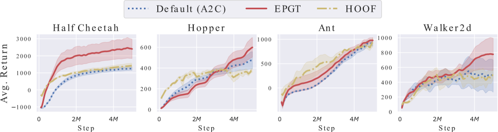
Figure 7: 4 Mujoco tasks: Average return over environmental steps across 10 training seeds using PG A2C.

4 mixed tasks with PG PPO

We use similar setting introduced in [28] using 4 tasks: BipedalWalker, LunarLanderContinous, Hopper and InvertedDoublePendulum, each is trained using 1 million environment steps. Here, 4 hyperparameters are optimized: learning rate $\alpha$, batch size $b$, GAE $\lambda$ and PPO clip $\epsilon$. The PG algorithm is PPO with configuration: $T=1600$, number of gradient updates=10, num workers=4, Adam optimizer with initial learning rate of $3\times 10^{-4}$ and $\gamma=0.99$ . Here, $\mathtt{T_{u}}=10\times 4\times 1600/b$ where $b$ is the batch size. The range of optimized hyperparameters: $b$ $\left\{128,256,512\right\}$, $\lambda$ $\left\{0.9,0.95,0.975,0.99\right\}$, $\epsilon$ $\left\{0.1,0.2,0.3,,0.5\right\}$, $\alpha$ using Eq. 5 with $\mathtt{B}=3$.

Fig. 8 compares the learning curves of EPGT against the baseline PPO with default hyperparameters. EPGT shows clear improvement in LunarLanderContinous and Hopper. We report EPGT’s numbers in Table 2 by using the best checkpoint to measure average return over 100 episodes for each run, then take median over 10 runs.

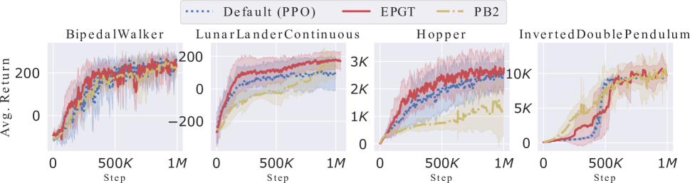
Figure 8: 4 tasks: Average return over environment steps across 10 training seeds using PG PPO.

Atari tasks with ACKTR

We adopt ACKTR as PG method with default hyperparameters [39]: number of workers=40, initial $\eta=0.25$, GAE $\lambda=0.95$, $\gamma=0.99$, $T=20$ and $\mathtt{U=10}$. The full set of tuned hyperparameters is trust region radius $\delta$ $\left\{0.001,0.002,0.003\right\}$, the value loss coefficient $l_{v}$$\left\{0.25,0.5,1.0\right\}$ and step size $\eta$ using Eq. 5 with $\mathtt{B}=3$.

Fig. 10 compares the learning curves of EPGT with different optimized hyperparameter set against the best ACKTR. The best ACKTR is found by grid-search ($\delta$ $\left\{0.001,0.003\right\}$, $l_{v}$$\left\{0.5,1.0\right\}$, $\eta\left\{0.2,0.07\right\}$) on Breakout. EPGT shows clear improvement in BeamRider, Qbert and SpaceInvaders.

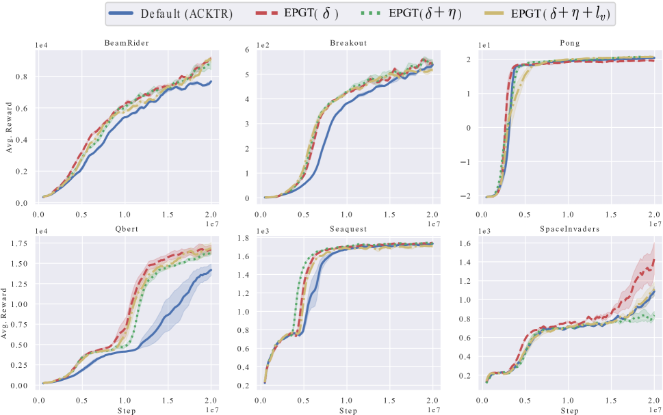
Figure 10: Atari games: Average return over environment steps across 5 training seeds using PG ACKTR.

Atari tasks with PPO

We adopt PPO as PG method with default hyperparameters [33]: $T=2048$, number of gradient updates=10, num workers=1, Adam optimizer with initial learning rate of $3\times 10^{-4}$ and $\gamma=0.99$ . Here, $\mathtt{U}=10\times 4\times 2048/b$ where $b$ is the batch size. The range of optimized hyperparameters: $b$ $\left\{128,256,512\right\}$, $\lambda$ $\left\{0.9,0.95,0.975,0.99\right\}$, $\epsilon$ $\left\{0.1,0.2,0.3,0.5\right\}$, $\alpha$ using Eq. 5 with $\mathtt{B}=3$.

Fig. 11 compares the learning curves of EPGT with different optimized hyperparameter set against the best PPO. The best PPO is found by grid-search ($b$ $\left\{128,256\right\}$, $\lambda$ $\left\{0.95,0.99\right\}$, $\epsilon$ $\left\{0.1,0.2\right\}$, $\alpha\left\{7\times 10^{-4},10^{-5}\right\}$) on Breakout. EPGT shows clear improvement in Breakout, Qbert, Seaquest and SpaceInvaders.

We note that we only perform grid-search on smaller hyperparameter value sets since grid-search is very expensive. EPGT only needs one run with similar training time as the original PG methods to achieve significantly better results than the best PG methods found after 16 runs of grid-search.

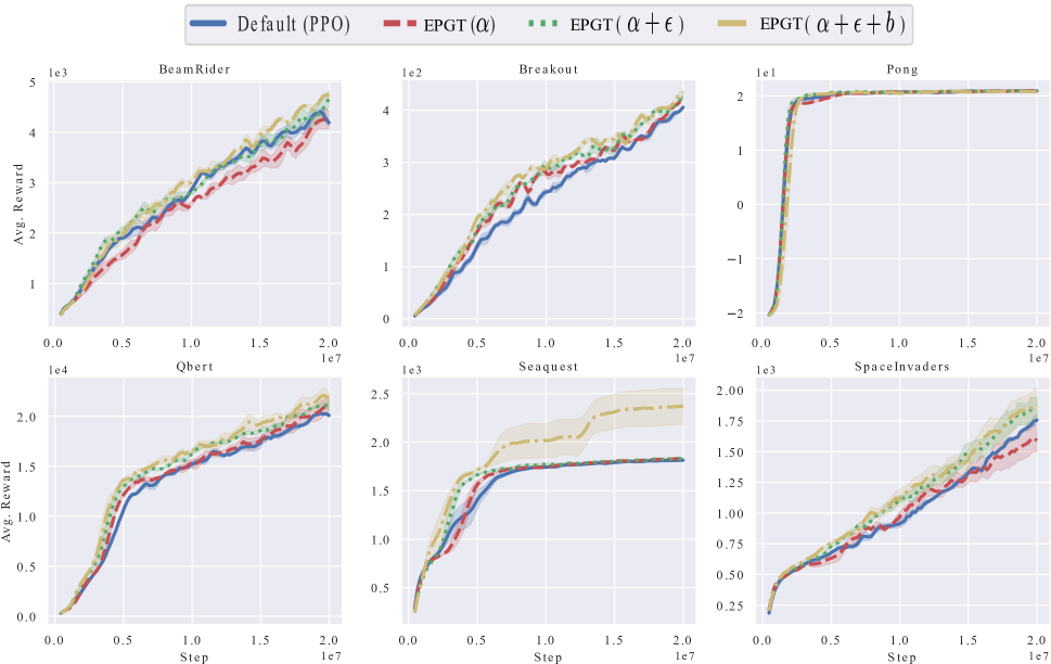
Figure 11: Atari games: Average return over environment steps across 5 training seeds using PG PPO.

6 Mujoco tasks with PPO

We adopt PPO as PG method with default hyperparameters [33]: number of workers=1, $T=2048$, $\gamma=0.99$, and Adam optimizer with initial learning rate of $3\times 10^{-4}$. Here, $\mathtt{U}=10\times 1\times 2048/b$. The full set of tuned hyperparameters is $b$ $\left\{128,256,512\right\}$, $\lambda$ $\left\{0.95,0.975,0.99\right\}$, $\epsilon$ $\left\{0.1,0.2,0.3\right\}$, $\alpha$ using Eq. 5 with $\mathtt{B}=3$.

Fig. 12 compares the learning curves of EPGT against the baseline default PPO and Random (RND) hyperparameter selection. EPGT shows clear improvement in HalfCheetah, Hopper, Walker2d and Humanoid.

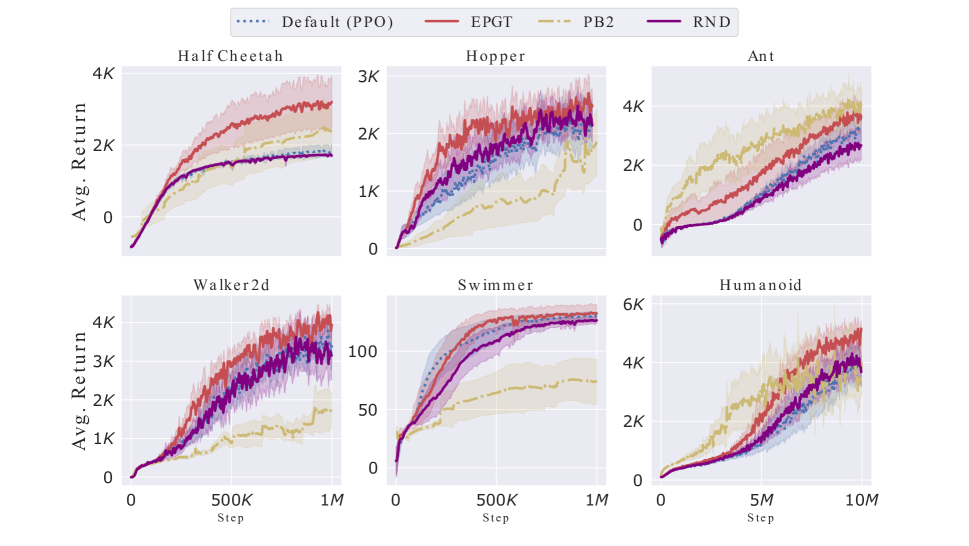
Figure 12: Mujoco: Average return over environment steps across 10 training seeds using PG PPO.

B.4 Details of ablation studies

Hyper-state size

Each tensor $W_{m}^{n}$ will be projected to a vector sized $d^{\prime}\times d$ where $d^{\prime}$ is the first dimension of $W_{m}^{n}$ and $d$ the last dimension of the mapping $C_{m}^{n}$. If the PG models has $M$ layers and we maintain $N_{order}$ orders of representations, the hyper-state vector’s size, in general, is $M\times N_{order}\times d^{\prime}\times d$. We already ablate $N_{order}$ in the main manuscript, $M$ and $d^{\prime}$ are fixed for each PG method, now we examine $d$.

Fig. 13 reports the ablation results. The common behavior is the performance improves when $N_{order}$ and $d$ increase to $N_{order}=2$ and $d=4$, which corresponds to $8K$-dimensional hyper-state vector in this experiment. When $N_{order}=0$, no derivative is used to represent the hyper-state, which leads to lower performance. When either $N_{order}$ or $d$ keeps growing, state vector size will be $16K$, which is too big for the episodic control method to work properly. For example, VAE almost cannot learn to minimize the reconstruction loss for $N_{order}=2$ and $d=8$ as shown in Fig. 13 (right).

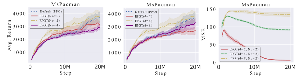
Figure 13: Ablation studies on order of representation $N_{order}$ (left) and projected size $d$ (middle). (Right) MSE loss of VAE model for different $d$. The curves are mean with std. over 5 runs.

Neighbor size K

We also test our model with different number of neighbors $K$ for both reading and writing. We use Atari game Demon Attack as an illustration and realize that $K=3$ is the best value (Fig. 14 (a)). More neighbors do not help because perhaps the cluster size of the similar-value representations is not big and thus, referring to far neighbors is not reliable.

Average vs Max writing rule

Traditional episodic controls [3] use max-rule as

$$\mathtt{M}\left(\phi\mathtt{\left(s^{\psi}\right)},\mathtt{a}_{i}^{\psi}\right)\leftarrow\max\left(\mathtt{M}\left(\phi\mathtt{\left(s^{\psi}\right)},\mathtt{a}_{i}^{\psi}\right),\mathtt{G}_{i}^{\psi}\right)$$

That stores the best experience the agent has so far and quickly guides next actions toward the best experience. However, this works only for near-deterministic environments as when $\mathtt{G}_{i}^{\psi}$ is unexpectedly high due to stochastic transition, a bad action is misunderstood as good one. This false belief may never be updated. Our Hyper-RL is not near-deterministic as the hyper-reward is basically MCMC estimation of the environment returns and the state is partially observable. Another problem of the max rule is it requires exact match to facilitate an update, which is rare in practice.

We address theses issue by taking weighted average and employing neighbor writing as in Eq. 4. As we write to multiple memory slots, it does not require exact match and enables fast value propagation inside the memory. Fig. 14 (b) shows the performance increase using the average compared to max rule in Atari Riverraid game.

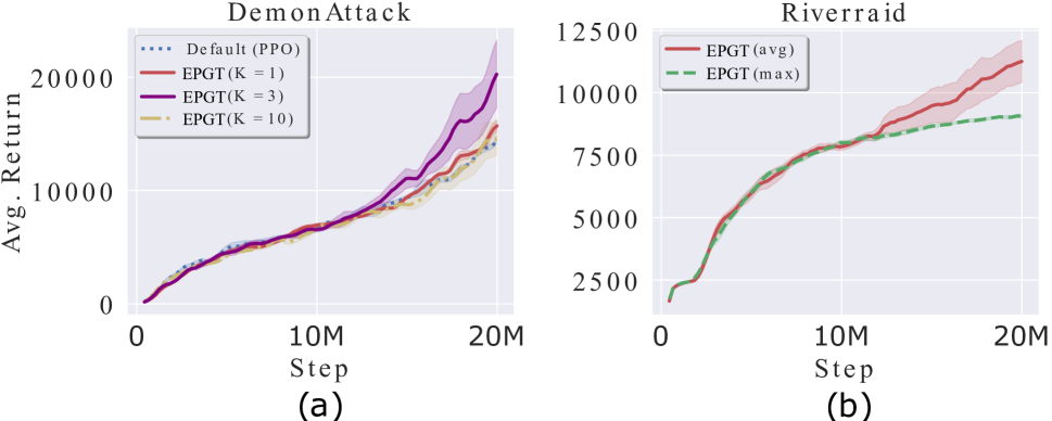
Figure 14: Ablation studies on neighbor size $K$ (a) and writing types (b). The curves are mean with std. over 5 runs.

C. Theoretical analysis of our writing rule

In this section, we show that using our writing, the value stored in the episodic memory is an approximation of the expected return (our writing is generic and can be used for general RL, hence we exclude “hyper-” in this section). The proof is based on [19]. In particular, we can always find $\beta$ such that the writing converges with probability $1$ and we also analyze the convergence as $\beta$ is constant, which is practically used in this paper.

To simplify the notation, we rewrite Eq. 4 as

$$\mathtt{M}_{i}\left(n+1\right)=\mathtt{M}_{i}\left(n\right)+\text{$\lambda\left(n\right)$}\left(\mathtt{G}_{j}\left(n\right)-\mathtt{M}_{i}\left(n\right)\right)$$ (6)

where $i$ and $j$ denote the current memory slot being updated and its neighbor that initiates the writing, respectively (it is opposite to the indices in Eq. 4). Here, the action is the same for both $i$ and $j$ slots, so we exclude action to simplify the notation. $\lambda\left(n\right)=\beta(n)\frac{Sim\left(i,j\right)}{\sum_{b=1}^{|\mathcal{N}(j)|}S_{bj}}$ where $\mathcal{N}\left(j\right)$ is the set of $K$ neighbors of $j$ slot. $\mathtt{G}_{j}$ is the return of the state-action whose key is the memory slot $j$, $Sim\left(j,i\right)$ the kernel function of 2 keys and $n$ the number of memory updates. This stochastic approximation converges when $\sum_{n=1}^{\infty}\lambda\left(n\right)=\infty$ and $\sum_{n=1}^{\infty}\lambda^{2}\left(n\right)<\infty$.

By definition, $Sim\left(i,j\right)=\frac{1}{\left\|\phi\left(\mathtt{s}_{i}^{\psi}\right)-\phi\left(\mathtt{s}_{j}^{\psi}\right)\right\|+\epsilon}$ and $\phi\left(\mathtt{s}^{\psi}\right)\leq 1$ since we use $\tanh$ activation in $\phi$. Hence, we have $\forall i,j$: $0<\frac{1}{2+\epsilon}\leq Sim\left(i,j\right)\leq\frac{1}{\epsilon}$. Hence, let $B_{ij}\left(n\right)$ a random variable denoting $\frac{Sim\left(i,j\right)}{\sum_{b=1}^{|\mathcal{N}(j)|}S_{bj}}$–the neighbor weight at step $n$, $\forall i,j:$

$$\frac{\epsilon}{K\epsilon+2K-2}\leq B_{ij}\left(n\right)\leq\frac{2+\epsilon}{K\epsilon+2}$$

That yields $\sum_{n=1}^{\infty}\lambda\left(n\right)\geq\frac{\epsilon}{K\epsilon+2K-2}\sum_{n=1}^{\infty}\beta\left(n\right)$ and $\sum_{n=1}^{\infty}\lambda^{2}\left(n\right)\leq\left(\frac{2+\epsilon}{K\epsilon+2}\right)^{2}\sum_{n=1}^{\infty}\beta^{2}\left(n\right)$. Hence the writing updates converge when $\sum_{n=1}^{\infty}\beta\left(n\right)=\infty$ and $\sum_{n=1}^{\infty}\beta^{2}\left(n\right)<\infty$. We can always choose such $\beta$ (e.g., $\beta\left(n\right)=\frac{1}{n+1}$).

With a constant writing rate $\beta$ ($\beta=1/2$), we rewrite Eq. 6 as

$$\mathtt{M}_{i}\left(n+1\right) =\mathtt{M}_{i}\left(n\right)+\beta B_{ij}\left(n\right)\left(\mathtt{G}_{j}\left(n\right)-\mathtt{M}_{i}\left(n\right)\right)$$

$$=\beta B_{ij}\left(n\right)\mathtt{G}_{j}\left(n\right)+\text{$\mathtt{M}_{i}\left(n\right)\left(1-\beta B_{ij}\left(n\right)\right)$}$$

$$=\sum_{t=1}^{n}\beta B_{ij}\left(t\right)\prod_{l=t+1}^{n}\left(1-\beta B_{ij}\left(l\right)\right)\mathtt{G}_{j}\left(t\right)$$

$$+\prod_{t=1}^{n}\left(1-\beta B_{ij}\left(t\right)\right)\mathtt{M}_{i}\left(1\right)$$

where the second term $\prod_{t=1}^{n}\left(1-\beta B_{ij}\left(t\right)\right)\mathtt{M}_{i}\left(1\right)\rightarrow 0$ as $n\rightarrow\infty$ since $B_{ij}\left(t\right)$ and $\beta$ are bounded between 0 and 1. The first term can be decomposed into three terms

$$\sum_{t=1}^{n}\beta B_{ij}\left(t\right)\prod_{l=t+1}^{n}\left(1-\beta B_{ij}\left(l\right)\right)\mathtt{G}_{j}\left(t\right) =T_{1}+T_{2}+T_{3}$$

where

$$T_{1} =\sum_{t=1}^{n}\beta B_{ij}\left(t\right)\prod_{l=t+1}^{n}\left(1-\beta B_{ij}\left(l\right)\right)Q_{i}$$

$$T_{2} =\sum_{t=1}^{n}\beta B_{ij}\left(t\right)\prod_{l=t+1}^{n}\left(1-\beta B_{ij}\left(l\right)\right)\Delta Q_{ij}\left(t\right)$$

$$T_{3} =\sum_{t=1}^{n}\beta B_{ij}\left(t\right)\prod_{l=t+1}^{n}\left(1-\beta B_{ij}\left(l\right)\right)\mathtt{\hat{G}}_{j}\left(t\right)$$

Here,$Q_{i}$ is the true action value of the state-action stored in slot $i$, $\Delta Q_{ij}\left(t\right)=Q_{j}\left(t\right)-Q_{i}$ and $\mathtt{\hat{G}}_{j}\left(t\right)=\mathtt{G}_{j}\left(t\right)-Q_{j}\left(t\right)$ the noise term between the return and the true action value. Assume that the action value is associated with zero mean noise and the action value noise is independent with the neighbor weights, then $\mathbb{E}\left(T_{3}\right)=0$.

Further, we make other two assumptions: (1) the neighbor weights are independent across update steps; (2) the probability $p_{j}$ of visiting a neighbor $j$ follows the same distribution across update steps and thus, $\mathbb{E}\left(B_{ij}\left(t\right)\right)=\mathbb{E}\left(B_{ij}\left(l\right)\right)=\mathbb{E}\left(B_{ij}\right)$. We now can compute

$$\mathbb{E}\left(T_{1}\right) =\mathbb{E}\left(\sum_{t=1}^{n}\beta B_{ij}\left(t\right)\prod_{l=t+1}^{n}\left(1-\beta B_{ij}\left(l\right)\right)Q_{i}\right)$$

$$=Q_{i}\sum_{t=1}^{n}\beta\mathbb{E}\left(B_{ij}\right)\prod_{l=t+1}^{n}\left(1-\alpha\mathbb{E}\left(B_{ij}\right)\right)$$

$$=Q_{i}\beta\mathbb{E}\left(B_{ij}\right)\sum_{t=1}^{n}\left(1-\beta\mathbb{E}\left(B_{ij}\right)\right)^{n-t}$$

$$=Q_{i}\beta\mathbb{E}\left(B_{ij}\right)\frac{1-\left(1-\beta\mathbb{E}\left(B_{ij}\right)\right)^{n}}{1-\left(1-\beta\mathbb{E}\left(B_{ij}\right)\right)}$$

$$=Q_{i}\left(1-\left(1-\beta\mathbb{E}\left(B_{ij}\right)\right)^{n}\right)$$

As $n\rightarrow\infty$, $\mathbb{E}\left(T_{1}\right)\rightarrow Q_{i}$ since since $B_{ij}\left(t\right)$ and $\alpha$ are bounded between 0 and 1.

Similarly, $\mathbb{E}\left(T_{3}\right)=\mathbb{E}\left(Q_{j}\left(t\right)-Q_{i}\right)=\mathbb{E}\left(Q_{j}\left(t\right)\right)-Q_{i}=\sum_{j=1}^{|\mathcal{N}(i)|}p_{j}Q_{j}-Q_{i}$, which is the approximation error of the KNN algorithm. Hence, with constant learning rate, on average, the $\mathtt{update}$ operator leads to the true action value (the expected return) plus the approximation error of KNN. The quality of KNN approximation determines the mean convergence of $\mathtt{update}$ operator. Since the bias-variance trade-off of KNN is specified by the number of neighbors $K$, choosing the right $K>1$ (not too big, not too small) is important to achieve good writing to ensure fast convergence. That explains why our writing to multiple slots ($K>1$) is generally better than the traditional writing to single slot ($K=1$).

References

- Bengio [2000] Bengio, Y. 2000. Gradient-based optimization of hyperparameters. Neural computation, 12(8): 1889–1900.
- Bergstra and Bengio [2012] Bergstra, J.; and Bengio, Y. 2012. Random search for hyper-parameter optimization. Journal of machine learning research, 13(2).
- Blundell et al. [2016] Blundell, C.; Uria, B.; Pritzel, A.; Li, Y.; Ruderman, A.; Leibo, J. Z.; Rae, J.; Wierstra, D.; and Hassabis, D. 2016. Model-free episodic control. arXiv preprint arXiv:1606.04460.
- Brochu, Cora, and De Freitas [2010] Brochu, E.; Cora, V. M.; and De Freitas, N. 2010. A tutorial on Bayesian optimization of expensive cost functions, with application to active user modeling and hierarchical reinforcement learning. arXiv preprint arXiv:1012.2599.
- Chen et al. [2018] Chen, Y.; Huang, A.; Wang, Z.; Antonoglou, I.; Schrittwieser, J.; Silver, D.; and de Freitas, N. 2018. Bayesian optimization in alphago. arXiv preprint arXiv:1812.06855.
- Duan et al. [2016] Duan, Y.; Chen, X.; Houthooft, R.; Schulman, J.; and Abbeel, P. 2016. Benchmarking deep reinforcement learning for continuous control. In International conference on machine learning, 1329–1338. PMLR.
- Fiszelew et al. [2007] Fiszelew, A.; Britos, P.; Ochoa, A.; Merlino, H.; Fernández, E.; and García-Martínez, R. 2007. Finding optimal neural network architecture using genetic algorithms. Advances in computer science and engineering research in computing science, 27: 15–24.
- Fujimoto, Hoof, and Meger [2018] Fujimoto, S.; Hoof, H.; and Meger, D. 2018. Addressing function approximation error in actor-critic methods. In International Conference on Machine Learning, 1587–1596. PMLR.
- González et al. [2016] González, J.; Dai, Z.; Hennig, P.; and Lawrence, N. 2016. Batch Bayesian optimization via local penalization. In Artificial intelligence and statistics, 648–657. PMLR.
- Henderson et al. [2018] Henderson, P.; Islam, R.; Bachman, P.; Pineau, J.; Precup, D.; and Meger, D. 2018. Deep reinforcement learning that matters. In Proceedings of the AAAI Conference on Artificial Intelligence, volume 32.
- Hung et al. [2019] Hung, C.-C.; Lillicrap, T.; Abramson, J.; Wu, Y.; Mirza, M.; Carnevale, F.; Ahuja, A.; and Wayne, G. 2019. Optimizing agent behavior over long time scales by transporting value. Nature communications, 10(1): 1–12.
- Hutter, Hoos, and Leyton-Brown [2011] Hutter, F.; Hoos, H. H.; and Leyton-Brown, K. 2011. Sequential model-based optimization for general algorithm configuration. In International conference on learning and intelligent optimization, 507–523. Springer.
- Hutter, Kotthoff, and Vanschoren [2019] Hutter, F.; Kotthoff, L.; and Vanschoren, J. 2019. Automated machine learning: methods, systems, challenges. Springer Nature.
- Jaderberg et al. [2017] Jaderberg, M.; Dalibard, V.; Osindero, S.; Czarnecki, W. M.; Donahue, J.; Razavi, A.; Vinyals, O.; Green, T.; Dunning, I.; Simonyan, K.; et al. 2017. Population based training of neural networks. arXiv preprint arXiv:1711.09846.
- Klein et al. [2017] Klein, A.; Falkner, S.; Bartels, S.; Hennig, P.; and Hutter, F. 2017. Fast bayesian optimization of machine learning hyperparameters on large datasets. In Artificial Intelligence and Statistics, 528–536. PMLR.
- Kohl and Stone [2004] Kohl, N.; and Stone, P. 2004. Policy gradient reinforcement learning for fast quadrupedal locomotion. In IEEE International Conference on Robotics and Automation, 2004. Proceedings. ICRA’04. 2004, volume 3, 2619–2624. IEEE.
- Kumaran, Hassabis, and McClelland [2016] Kumaran, D.; Hassabis, D.; and McClelland, J. L. 2016. What learning systems do intelligent agents need? Complementary learning systems theory updated. Trends in cognitive sciences, 20(7): 512–534.
- Larochelle et al. [2007] Larochelle, H.; Erhan, D.; Courville, A.; Bergstra, J.; and Bengio, Y. 2007. An empirical evaluation of deep architectures on problems with many factors of variation. In Proceedings of the 24th international conference on Machine learning, 473–480.
- Le et al. [2021] Le, H.; George, T. K.; Abdolshah, M.; Tran, T.; and Venkatesh, S. 2021. Model-Based Episodic Memory Induces Dynamic Hybrid Controls. In Thirty-Fifth Conference on Neural Information Processing Systems.
- Le, Tran, and Venkatesh [2019] Le, H.; Tran, T.; and Venkatesh, S. 2019. Learning to remember more with less memorization. In Proceedings of the 7th International Conference on Learning Representations.
- Le, Tran, and Venkatesh [2020] Le, H.; Tran, T.; and Venkatesh, S. 2020. Self-Attentive Associative Memory. In Proceedings of the 37th International Conference on Machine Learning.
- Le and Venkatesh [2020] Le, H.; and Venkatesh, S. 2020. Neurocoder: Learning General-Purpose Computation Using Stored Neural Programs. arXiv preprint arXiv:2009.11443.
- Lengyel and Dayan [2008] Lengyel, M.; and Dayan, P. 2008. Hippocampal contributions to control: the third way. In Advances in neural information processing systems, 889–896.
- Li et al. [2019] Li, A.; Spyra, O.; Perel, S.; Dalibard, V.; Jaderberg, M.; Gu, C.; Budden, D.; Harley, T.; and Gupta, P. 2019. A generalized framework for population based training. In Proceedings of the 25th ACM SIGKDD International Conference on Knowledge Discovery & Data Mining, 1791–1799.
- Luketina et al. [2016] Luketina, J.; Berglund, M.; Greff, K.; and Raiko, T. 2016. Scalable gradient-based tuning of continuous regularization hyperparameters. In International conference on machine learning, 2952–2960. PMLR.
- Mnih et al. [2016] Mnih, V.; Badia, A. P.; Mirza, M.; Graves, A.; Lillicrap, T.; Harley, T.; Silver, D.; and Kavukcuoglu, K. 2016. Asynchronous methods for deep reinforcement learning. In International conference on machine learning, 1928–1937. PMLR.
- Mnih et al. [2015] Mnih, V.; Kavukcuoglu, K.; Silver, D.; Rusu, A. A.; Veness, J.; Bellemare, M. G.; Graves, A.; Riedmiller, M.; Fidjeland, A. K.; Ostrovski, G.; et al. 2015. Human-level control through deep reinforcement learning. nature, 518(7540): 529–533.
- Parker-Holder, Nguyen, and Roberts [2020] Parker-Holder, J.; Nguyen, V.; and Roberts, S. J. 2020. Provably efficient online hyperparameter optimization with population-based bandits. Advances in Neural Information Processing Systems, 33.
- Paul, Kurin, and Whiteson [2019] Paul, S.; Kurin, V.; and Whiteson, S. 2019. Fast Efficient Hyperparameter Tuning for Policy Gradient Methods. In Wallach, H.; Larochelle, H.; Beygelzimer, A.; d'Alché-Buc, F.; Fox, E.; and Garnett, R., eds., Advances in Neural Information Processing Systems, volume 32. Curran Associates, Inc.
- Peters and Schaal [2006] Peters, J.; and Schaal, S. 2006. Policy gradient methods for robotics. In 2006 IEEE/RSJ International Conference on Intelligent Robots and Systems, 2219–2225. IEEE.
- Pritzel et al. [2017] Pritzel, A.; Uria, B.; Srinivasan, S.; Badia, A. P.; Vinyals, O.; Hassabis, D.; Wierstra, D.; and Blundell, C. 2017. Neural episodic control. In Proceedings of the 34th International Conference on Machine Learning-Volume 70, 2827–2836. JMLR. org.
- Rana et al. [2017] Rana, S.; Li, C.; Gupta, S.; Nguyen, V.; and Venkatesh, S. 2017. High dimensional Bayesian optimization with elastic Gaussian process. In International conference on machine learning, 2883–2891. PMLR.
- Schulman et al. [2017] Schulman, J.; Wolski, F.; Dhariwal, P.; Radford, A.; and Klimov, O. 2017. Proximal policy optimization algorithms. arXiv preprint arXiv:1707.06347.
- Silver et al. [2017] Silver, D.; Schrittwieser, J.; Simonyan, K.; Antonoglou, I.; Huang, A.; Guez, A.; Hubert, T.; Baker, L.; Lai, M.; Bolton, A.; et al. 2017. Mastering the game of go without human knowledge. nature, 550(7676): 354–359.
- Snoek, Larochelle, and Adams [2012] Snoek, J.; Larochelle, H.; and Adams, R. P. 2012. Practical Bayesian optimization of machine learning algorithms. In Proceedings of the 25th International Conference on Neural Information Processing Systems-Volume 2, 2951–2959.
- Sutton [1992] Sutton, R. S. 1992. Adapting bias by gradient descent: An incremental version of delta-bar-delta. In AAAI, 171–176. San Jose, CA.
- Tang and Choromanski [2020] Tang, Y.; and Choromanski, K. 2020. Online hyper-parameter tuning in off-policy learning via evolutionary strategies. arXiv preprint arXiv:2006.07554.
- Tulving [2002] Tulving, E. 2002. Episodic memory: From mind to brain. Annual review of psychology, 53(1): 1–25.
- Wu et al. [2017] Wu, Y.; Mansimov, E.; Liao, S.; Grosse, R.; and Ba, J. 2017. Scalable trust-region method for deep reinforcement learning using Kronecker-factored approximation. In Proceedings of the 31st International Conference on Neural Information Processing Systems, 5285–5294.
- Xu, van Hasselt, and Silver [2018] Xu, Z.; van Hasselt, H. P.; and Silver, D. 2018. Meta-Gradient Reinforcement Learning. Advances in Neural Information Processing Systems, 31: 2396–2407.
- Young et al. [2015] Young, S. R.; Rose, D. C.; Karnowski, T. P.; Lim, S.-H.; and Patton, R. M. 2015. Optimizing deep learning hyper-parameters through an evolutionary algorithm. In Proceedings of the Workshop on Machine Learning in High-Performance Computing Environments, 1–5.
- Zhang et al. [2021] Zhang, B.; Rajan, R.; Pineda, L.; Lambert, N.; Biedenkapp, A.; Chua, K.; Hutter, F.; and Calandra, R. 2021. On the importance of hyperparameter optimization for model-based reinforcement learning. In International Conference on Artificial Intelligence and Statistics, 4015–4023. PMLR.
- Ziegler et al. [2019] Ziegler, D. M.; Stiennon, N.; Wu, J.; Brown, T. B.; Radford, A.; Amodei, D.; Christiano, P.; and Irving, G. 2019. Fine-tuning language models from human preferences. arXiv preprint arXiv:1909.08593.