Inference for ROC Curves Based on Estimated Predictive Indices

Abstract

We provide a comprehensive theory of conducting in-sample statistical inference about receiver operating characteristic (ROC) curves that are based on predicted values from a first stage model with estimated parameters (such as a logit regression). The term “in-sample” refers to the practice of using the same data for model estimation (training) and subsequent evaluation, i.e., the construction of the ROC curve. We show that in this case the first stage estimation error has a generally non-negligible impact on the asymptotic distribution of the ROC curve and develop the appropriate pointwise and functional limit theory. We propose methods for simulating the distribution of the limit process and show how to use the results in practice in comparing ROC curves.

Keywords: classification, ROC curve, uniform asymptotics, estimation effect

JEL codes: C25, C38, C46, C52

1 Introduction

Binary prediction or classification is a fundamental problem in statistics and machine learning with applications in many scientific disciplines including economics. The predictive ability of statistical models used for binary classification is frequently evaluated through the receiver operating characteristic (ROC) curve, designed to summarize the tradeoffs between the probability of a true positive prediction (vertical axis) and a false positive prediction (horizontal axis) as one combines a predictive index with a varying classification threshold. Though its origins are in the signal detection and medical diagnostics literature, in recent years ROC analysis has become increasingly common in financial and economic applications as well (e.g., Anjali and Bossaerts 2014; Bazzi et al. 2021; Bonfim et al. 2021; Berge and Jorda 2011; Kleinberg et al. 2018; Lahiri and Wang 2013; Lahiri and Yang 2018; McCracken et al. 2021; Schularik and Taylor 2012 and many others).

While there is a large literature on the statistical properties of empirical ROC curves, the standard distributional theory assumes that the signal or predicitive index used for classification is either directly observed—it is “raw data”—or that it is a fixed function of raw data. However, if the signal itself is generated from an underlying regression model with estimated coefficients, conducting in-sample inference about ROC curves based on the traditional theory can be highly misleading. For instance, Demler et al. (2012) point out that the standard DeLong et al. (1988) test for comparing AUCs for different (but potentially correlated) signals can lead to flawed inference if the signals come from nested models with estimated coefficients. Similarly, Lieli and Hsu (2019) demonstrate that the asymptotic normality results in Bamber (1975) are inappropriate for testing AUC=1/2 for models with estimated parameters.

The central contribution of this paper is the development of a general functional limit theory for the empirical ROC curve that takes the pre-estimation effect into account. Regarding the ROC curve as a random function defined over the [0,1] interval, we provide a uniform influence function representation theorem, and show that the difference between the empirical and population ROC curves converges weakly to a mean zero Gaussian process with a given covariance structure at the parametric rate. These results constitute a non-trivial extension of the functional limit result in Hsieh and Turnbull (1996), who work under the assumption that the observations available on the predictive index are i.i.d. conditional on the outcome. (If the predictive index depends on coefficients estimated in-sample, this assumption is no longer valid, as the parameter estimates depend on all data points.) Our results not only allow for the construction of a uniform confidence band for the ROC curve but also facilitate model selection through handling virtually any comparison between two correlated ROC curves (e.g., testing dominance or partial dominance; testing the difference between AUCs or partial AUCs, etc.) In terms implementation, we propose two methods to simulate the limiting distribution of the empirical ROC curve, one of which is the weighted bootstrap by Ma and Kosorok (2005). Although some type of bootstrap procedure would be a natural way to approach the pre-estimation problem in practice even without a theory, our results provide rigorous justification and guidance for doing this.

A second contribution of the theory developed in this paper is that it provides insight into what determines the impact of the first stage estimation error on the asymptotic distribution of the ROC curve. The derivatives of the true and false positive prediction rates with respect to the first stage model parameters play a central role — if these gradients vanish at the pseudo-true parameter values, then so does the estimation effect. Nevertheless, the gradients also depend on the classification threshold and will not generally be negligible along the entire ROC curve. For associated functionals, it is the gradient of the functional that drives the estimation effect. Some functionals, e.g., the area under the curve, have the property that they are maximal when the predictive index is given by $p(X)=P(Y=1|X)$, the conditional probability of a positive outcome $Y$ given the covariates $X$. For such functionals the estimation effect is negligible when the first stage model is correctly specified for $p(X)$ and the first stage estimator converges at the root-n rate. Nevertheless, the first stage estimation error will generally affect the asymptotic distribution under misspecification; thus, our results facilitate robust inference.

There are additional technical contributions that are more subtle. In employing standard empirical process techniques to derive our results, we make most of the fact that the population and sample ROC curves are invariant to monotone increasing transformations of the predictive index. This observation allows us to leverage powerful assumptions that may seem restrictive at first glance. In particular, we use the assumption that the density $f_{0}$ of the predictive index conditional on $Y=0$ is bounded away from zero to derive various uniform approximations. The problem is that even if the individual predictors have densities bounded away from zero (already a big if), the predictive index may not share this property, as it often involves a linear combination of the predictors. Nevertheless, one can always find a strictly increasing transformation of the predictive index, say, the probability integral transform, so that the post-transform $f_{0}$ will be greater than some $\epsilon>0$ across the whole support. What matters for the asymptotic theory is the properties of the likelihood ratio $f_{1}/f_{0}$, which is invariant to monotone increasing transformations (here $f_{1}$ is the conditional density of the predictive index given $Y=1$). In particular, uniform inference is possible only for parts of the ROC curve that are generated by thresholds falling into some interval $[c_{L},c_{U}]$ over which $f_{1}/f_{0}$ is bounded and bounded away from zero. But given the properties of the likelihood ratio, one is free to assume the theoretically most convenient scenario about the individual density $f_{0}$ that is achievable through monotone transformations, even if this transformation is not implemented or even identified.

We must also point out some technical limitations of the paper. First, we do not allow for serial dependence in the data, precluding time series applications such as the evaluation of recession forecasting models. Nevertheless, our proofs rely mostly on high level conditions; specifically, the asymptotically linear representation of the first stage estimator, the stochastic equicontinuity of the empirical process defined by the (pseudo-true) predictive index, and the uniform continuity of some derivatives. Given the availability of these conditions for stationary, weakly dependent time series, we conjecture that our representation results should generalize to this setting with relatively straightforward modifications. However, simulating the asymptotic distribution of the limiting process would require more complex procedures and we do not pursue this extension here. Second, the predictive model evaluated at the pseudo-true parameter values must have strictly positive variance. This is not an innocent assumption in that it rules out a completely uninformative predictive model. For example, our results are not suitable for testing the hypothesis that AUC=1/2; see Lieli and Hsu (2019) for some specialized results in this very non-standard case. More generally, in using our results to compare two ROC curves, the difference of the two influence functions evaluated at the pseudo-true parameter values must have strictly positive variance as well. This condition can be violated when the first stage models are nested, and we are currently working on some test procedures that are applicable in this scenario as well. Finally, we only consider parametric estimators of $p(X)$ as the first stage model; nonparametric estimators that converge slower than the root-n rate are ruled out.

One might discount the practical relevance of our theoretical results discussed above based on the fact that the first stage estimation problem can be avoided by conducting out-of-sample evaluation. If the ROC curve is constructed over a test sample that is independent of the training sample used to estimate the first stage model, then the asymptotic validity of the standard inference procedures is restored. We acknowledge this point but offer two responses. First, out-of-sample evaluation is costly: it leads to power loss in model comparisons and the potential dependence of the results on the particular split(s) used. In fact, one could argue that out-of-sample evaluation is a necessity forced on practitioners by the fact that it is often very difficult to characterize analytically or in a practically useful way how goodness-of-fit measures behave over the training sample so that one can compensate for overfitting. In this case we do provide such a result. Second, apart from dealing with the pre-estimation problem, our results provide a unified framework for conducting uniform inference, and comparing ROC curves estimated over the same sample in virtually any way.

This work has ties to several strands of the statistics and econometrics literature. We have already cited a number of classic works on the statistical properties of the empirical ROC curve that maintain the assumption of a directly observed signal (Bamber 1975, DeLong et al. 1988, Hsieh and Turnbull 1996). It is the last of these papers that is closest to ours; however, the pre-estimation effect is obviously missing from their framework and they actually do not exploit their functional limit result for inference apart from re-deriving the asymptotic normality result of Bamber (1975) for the empirical AUC. Instead, they focus on estimating the ROC curve under an additional “binormal” assumption, i.e., when the signal has a normal distribution conditional on both outcomes.

Pre-estimation problems have a long history in the literature; for example, Pagan (1984) studied the distributional consequences of including “generated regressors” into a regression model. As mentioned above, Demler et al. (2012) pointed out the relevance of the pre-estimation effect in the context of ROC analysis. More generally, our work is related to papers dealing with two-step estimators where the first step involves estimating some nuisance parameter whose sampling variation potentially affects the otherwise well-understood second stage. Abadie and Imbens (2016) is a relatively recent example in the context of matching estimators.

The application of our results in testing for dominance relations and AUC differences across ROC curves has similarities to stochastic dominance tests; see, e.g., Barrett and Donald (2003), Linton, Maasoumi and Whang (2005), Linton, Song and Whang (2010) and Donald and Hsu (2016). Some papers, such as Linton, Maasoumi and Whang (2005) and Linton, Song and Whang (2010), even allow for generated variables in this context. Finally, the paper speaks indirectly to the forecasting literature on the relative merits of in-sample vs. out-of-sample model evaluation (e.g., Inoue and Kilian 2004, Clark and McCracken 2012). The connection lies in the fact that we extend the scope of in-sample evaluation methods in binary prediction.

The rest of the paper is organized as follows. Section 2 sets up the prediction framework and introduces the ROC curve along with some of its basic properties. Section 3 discusses the estimation effect in detail and presents pointwise (fixed-cutoff) asymptotic results. The functional limit theory is contained in Section 4. In Section 5 we show how to use the abstract results for conducting inference about the ROC curve; we discuss dominance testing, AUC comparisons, etc. Section 6 presents Monte Carlo results highlighting the impact of first stage estimation on the distribution of the ROC curve. Section 7 concludes.

2 Making and evaluating binary predictions

2.1 Cutoff rules and the ROC curve

Let $Y\in\{0,1\}$ be a Bernoulli random variable representing some outcome of interest and $X$ be a $k\times 1$ vector of covariates (predictors). We consider point forecasts (classifications) of $Y$ that are constructed by combining a scalar predictive index $G(X)$ with a suitable cutoff (threshold) $c$. More specifically, the prediction rule for $Y$ is given by

$$\hat{Y}(c)=1[G(X)>c],$$ (1)

where $1[.]$ is the indicator function. The role of the function $G:\mathbb{R}^{k}\rightarrow\mathbb{R}$ is to aggregate the information that the predictors contain about $Y$ while the choice of $c$ governs the use of this information. With $G$ and $c$ unrestricted, (1) represents a very general class of prediction rules.

In many binary prediction problems there is also a loss function $\ell(\hat{y},y)$ that describes the cost of predicting $Y=\hat{y}$ when the realized outcome is $Y=y$. If the decision maker’s objective is to minimize expected loss conditional on $X$, the optimal choice of $G$ and $c$ is determined as follows. Given the observed value of $X$, the optimal point forecast of $Y$ solves

$$\min_{\hat{y}\in\{0,1\}}E[\ell(\hat{y},Y)|X]=\min_{\hat{y}\in\{0,1\}}\big{[}\ell(\hat{y},1)p(X)+\ell(\hat{y},0)(1-p(X))\big{]},$$ (2)

where $p(X)=\mathbb{P}(Y=1|X)$ is the conditional probability of $Y=1$ given $X$. Adopting the normalization $\ell(0,0)=\ell(1,1)=0$ and assuming $\ell(0,1)>0$ and $\ell(1,0)>0$, it is straightforward to verify that the optimal prediction rule is given by

$$\hat{Y}^{*}(c_{\ell})=1[p(X)>c_{\ell}],$$ (3)

where $c_{\ell}=\ell(1,0)/[\ell(0,1)+\ell(1,0)]$.

Equation (3) reveals that the optimal predictive index is $p(X)$ regardless of $\ell$ while the optimal choice of $c$ is fully determined by $\ell$ (specifically, by the relative cost of a false alarm versus a miss). This simple observation motivates a two-step empirical strategy in binary prediction. First, one models and estimates $p(X)$ using data on $(Y,X)$; a common approach is to specify a parametric model $G(X,\beta)$ for $p(X)$ and to estimate it by maximum likelihood (logistic regression is a leading example). In the second step a point forecast is obtained by combining the estimated conditional probability $G(X,\hat{\beta})$ with a suitable cutoff, which depends on the forecaster’s or forecaster user’s preferences. Thus, there is a separation between the construction of the predictive index, representing the objective information available to the forecaster, and the use of that information, governed by the loss function.

We will now define the population receiver operating characteristic (ROC) curve. Let $G(X,\beta)$ be a predictive index with a fixed value of the parameter $\beta$. Combined with a cutoff $c$, the resulting prediction rule produces true positive predictions and false positive predictions (false alarms) with the following probabilities:

$$TP(c,\beta) = \mathbb{P}[\hat{Y}(c)=1|\,Y=1]=\mathbb{P}[G(X,\beta)>c|\,Y=1]$$

$$FP(c,\beta) = \mathbb{P}[\hat{Y}(c)=1|\,Y=0]=\mathbb{P}[G(X,\beta)>c|\,Y=0],$$

where TP and FP stand for the rate of “true positive” and “false positive” predictions, respectively. As the cutoff $c$ varies, both quantities change in the same direction; in general, TP can be increased only at the cost of increasing FP as well. The ROC curve traces out all attainable (FP, TP) pairs in the $[0,1]\times[0,1]$ unit square, i.e., it is the locus

$$\Big{\{}\big{(}FP(c,\beta),TP(c,\beta)\big{)}:c\in\mathbb{R}\Big{\}}.$$

Intuitively, the ROC curve is a way of summarizing the information content of $G(X,\beta)$ about the outcome $Y$ without committing to any particular cutoff, i.e., loss function. The use of such a forecast evaluation tool is particularly appropriate in situations in which there many potential forecast users with diverse loss functions; see Lieli and Nieto-Barthaburu (2010). It is also clear from the definition that the ROC curve is invariant to strictly monotone transformations of $G(X,\beta)$.

The ROC curve based on the true conditional probability function $p(X)$ possesses some optimality properties. To state these in a parametric modeling framework, we introduce the following correct specification assumption.

Assumption 1 There exists some point $\beta^{\circ}$ in the parameter space $\mathcal{B}\subseteq\mathbb{R}^{p}$ such that $G(X,\beta^{\circ})=p(X)$ almost surely.

We state the following result.

Proposition 1

(i) Given Assumption 2.1, $\beta^{\circ}$ solves the following maximization problem for any value of $c$:

$$\max_{\beta}\big{[}(1-c)\pi TP(c,\beta)-c(1-\pi)FP(c,\beta)\big{]},$$

where $\pi=\mathbb{P}(Y=1)$.

(ii) Given Assumption 2.1, define $F^{\circ}_{c}=FP(c,\beta^{\circ})$. Then $\beta^{\circ}$ also solves the following constrained maximization problem for any value of $c$:

$$\max_{\beta}TP(c,\beta)\text{ s.t. }FP(c,\beta)=F^{\circ}_{c}$$

Remarks:

1. Part (i) is a consequence of the predictor (3) solving (2) for any given value of $X$. To see this, note that by the law of iterated expectations and the monotonicity of the expectation operator, $\hat{Y}^{*}(c_{\ell})$ also solves the unconditional expected loss minimization problem $\min_{\hat{Y}}E_{XY}[\ell(\hat{Y},Y)]$, where the minimization is over all random variables $\hat{Y}$ that are (measurable) transformations of $X$. It is easy to verify that $E[\ell(\hat{Y},Y)]$ can be written as

   $$[\ell(0,1)+\ell(1,0)]\cdot\big{[}c_{\ell}(1-\pi)\mathbb{P}(\hat{Y}=1|\,Y=0)-(1-c_{\ell})\pi\mathbb{P}(\hat{Y}=1|\,Y=1)\big{]}+\pi\ell(0,1),$$

   which immediately implies the result.

2. Part (ii) is a consequence of part (i) and it means that for any given FP rate, it is the ROC curve based on $p(X)$ that achieves the largest possible TP rate. In other words, the ROC curve associated with $p(X)$ weakly dominates any other ROC curve that is constructed based on some index $G(X)$.

3. These results are not new; they have appeared in the ROC literature in alternative formulations. See, e.g., Egan (1975) and Pepe (2003, Section 4).

2.2 The sample ROC curve and conventional inference

Throughout the paper we maintain the assumption that the available data consists of a random sample. More formally:

Assumption 2 The sample $\{(Y_{i},X_{i})\}_{i=1}^{n}$ consists of independent and identically distributed observations on the random vector $(Y,X)\in\{0,1\}\times\mathbb{R}^{k}$.

Given the sample and a fixed value of $\beta$, the empirical ROC curve is defined as the locus $\big{\{}(\widehat{FP}(c,\beta),\widehat{TP}(c,\beta)):c\in\mathbb{R}\big{\}}\subset[0,1]\times[0,1]$, where

$$\widehat{TP}(c,\beta) = \frac{1}{n_{1}}\sum_{i=1}^{n}1[G(X_{i},\beta)>c,Y_{i}=1]$$

$$\widehat{FP}(c,\beta) = \frac{1}{n_{0}}\sum_{i=1}^{n}1[G(X_{i},\beta)>c,Y_{i}=0],$$

and $n_{1}=\sum_{i=1}^{n}Y_{i}$, $n_{0}=n-n_{1}$.

The simplest type of inference about an ROC curve involves constructing (joint) confidence intervals for $TP(c,\beta)$ and $FP(c,\beta)$ for one threshold $c$ at a time and for fixed values of the coefficient vector $\beta$. In this case one can use the CLT to arrive at the normal approximations:

$$\sqrt{n}[\widehat{TP}(c,\beta)-TP(c,\beta)]\rightarrow_{d}N\big{[}0,TP(1-TP)/\pi\big{]}$$ (4)

$$\sqrt{n}[\widehat{FP}(c,\beta)-FP(c,\beta)]\rightarrow_{d}N\big{[}0,FP(1-FP)/(1-\pi)\big{]},$$ (5)

where TP is a shorthand for $TP(c,\beta)$ (and similarly for FP). These results immediately provide asymptotic confidence intervals for TP and FP, and a joint confidence rectangle is also easy to construct due to the independence of $\widehat{TP}(c,\beta)$ and $\widehat{FP}(c,\beta)$; see Pepe (2003), Section 2.2.2 for details.

Furthermore, for fixed $\beta$ one can apply the asymptotic normality results in Bamber (1975) to conduct inference about the AUC, and the DeLong et. al. (1988) test for comparing the areas under ROC curves based on different (but non-random) values of $\beta$. The nonparametric functional limit result in Hsieh and Turnbull (1996) also applies.

3 In-sample inference: pointwise asymptotics

We will now develop a comprehensive theory of in-sample inference about individual points on the ROC curve taking the pre-estimation effect into account. We present both analytical results and results based on the weighted bootstrap. We start by describing the setup and stating some technical conditions.

3.1 First stage estimation and technical assumptions

The sample $\{(Y_{i},X_{i})\}_{i=1}^{n}$ now plays a dual role. First, it is used to construct an estimated parameter vector $\hat{\beta}=\hat{\beta}_{n}$. Typically, $\hat{\beta}$ consists of an intercept and slope coefficients from some type of regression of $Y$ on $X$ (e.g., linear, logit or probit). Second, the same sample is used to compute the predictive index values $G(X_{i},\hat{\beta})$, $i=1,\ldots,n$, and to construct the empirical ROC curve as described in Section 2.2. We impose the following high level condition on $\hat{\beta}$.

Assumption 3 (i) Let $\hat{\beta}$ be an M-estimator of $\beta$ so that

$$\hat{\beta}\equiv\arg\max_{\beta\in\mathcal{B}}\frac{1}{n}\sum_{i=1}^{n}q(Y_{i},X_{i},\beta).$$

(ii) There is a point $\beta^{*}$ in the interior of the compact parameter space $\mathcal{B}\subset\mathbb{R}^{p}$ so that

$$\sqrt{n}(\hat{\beta}_{n}-\beta^{*})=\frac{1}{\sqrt{n}}\sum_{i=1}^{n}\psi_{\beta}(Y_{i},X_{i},\beta^{*})+o_{p}(1),$$ (6)

where $\psi_{\beta}:\mathbb{R}^{1+k+p}\rightarrow\mathbb{R}^{p}$ is a given function with $E[\psi_{\beta}(Y,X,\beta^{*})]=0$ and $E\|\psi_{\beta}(Y,X,\beta^{*})\|^{2+\epsilon}<\infty$ for some $\epsilon>0$. Furthermore, $\beta^{*}=\beta^{\circ}$ under Assumption 2.1.

Assumption 3.1 states that $\hat{\beta}$ is an $M$-estimator with an asymptotically linear representation, implying that $\hat{\beta}$ is asymptotically normally distributed. The stated conditions do not require the first stage model to be correctly specified for $p(X)$; $\beta^{*}$ simply stands for the probability limit of $\hat{\beta}$, i.e., the pseudo-true value of the parameter vector. We nevertheless assume that $\hat{\beta}$ is consistent for $\beta^{\circ}$ under correct specification (Assumption 2.1). The reason for allowing for misspecification is twofold. First, the first stage predictive model is often simply an approximation of $p(X)$, e.g., a linear regression. Second, as we will see, the estimation effect can depend on whether or not the model is correctly specified.

Assumption 4 The empirical processes

$$(c,\beta)\mapsto\sqrt{n}(\hat{\mathbb{P}}_{0}-\mathbb{P}_{0})1[G(X,\beta)\leq c]\text{ and }(c,\beta)\mapsto\sqrt{n}(\hat{\mathbb{P}}_{1}-\mathbb{P}_{1})1[G(X,\beta)\leq c]$$

are stochastically equicontinuous over $\mathbb{R}\times\mathcal{B}$, where $\mathbb{P}_{j}$ denotes probability conditional on $Y=j$ and $\hat{\mathbb{P}}_{j}$ is the corresponding empirical measure in the $Y=j$ subsample.

The stochastic equicontinuity requirement in Assumption 3.1 limits the complexity of the model $G(X,\beta)$ and plays an important role in handling the estimation effect. It holds, for example, if $G(X,\beta)=X^{\prime}\beta$ or $G(X,\beta)=G(X^{\prime}\beta)$ with $G$ bounded (see the definition of a type I class in Andrews 1994). Apart from a small degree of added generality, we state stochastic equicontinuity as a high level condition to make it more transparent what is required for our results.

The final assumption states the differentiability of $TP$ and $FP$ with respect to the components of $\beta$. Let $\nabla_{\beta}$ denote the corresponding gradient operator and $B^{*}(r)$ the open ball with radius $r>0$ centered on $\beta^{*}$.

Assumption 5 For any given cutoff $c$, the gradient vectors $\nabla_{\beta}TP(c,\beta)$ and $\nabla_{\beta}FP(c,\beta)$ exist and are continuous over $B^{*}(r)$ for some $r>0$.

As we will shortly see, the first stage estimation of $\beta$ affects the asymptotic distribution of the ROC curve through the derivatives presented in Assumption 3.1.

3.2 Theoretical illustration of the estimation effect

Let $c$ be a given value of the cutoff; we want to conduct inference about the corresponding point $(FP(c,\beta^{*}),TP(c,\beta^{*}))$ on the limiting ROC curve. To isolate the effect of the first stage estimator $\hat{\beta}$ on the asymptotic distribution of $\widehat{TP}(c,\hat{\beta})$, we can write

$$\sqrt{n}[\widehat{TP}(c,\hat{\beta})-TP(c,\beta^{*})]$$

$$=\sqrt{n}[\widehat{TP}(c,\hat{\beta})-TP(c,\hat{\beta})]+\sqrt{n}[TP(c,\hat{\beta})-TP(c,\beta^{*})]$$

$$=\sqrt{n}[\widehat{TP}(c,\beta^{*})-TP(c,\beta^{*})]+\sqrt{n}[TP(c,\hat{\beta})-TP(c,\beta^{*})]+o_{p}(1),$$ (7)

where the second equality is due to the fact that the process $\sqrt{n}(\widehat{TP}-TP)$ is stochastically equicontinuous (Assumption 3.1), implying

$$\sqrt{n}[\widehat{TP}(c,\hat{\beta})-TP(c,\hat{\beta})]-\sqrt{n}[\widehat{TP}(c,\beta^{*})-TP(c,\beta^{*})]=o_{p}(1),$$

given that $\hat{\beta}\rightarrow_{p}\beta^{*}$. As $\beta^{*}$ is fixed and $Var[G(X,\beta^{*})]>0$, the first term in equation (7) has the asymptotic distribution given by (4) and the second term represents the effect of estimating $\beta^{*}$. Does this term have a non-negligible effect on the asymptotic distribution of $\widehat{TP}(c,\hat{\beta})$, and if yes, how do we characterize it?

To address these questions, we can use Assumption 3.1 to expand the second term in (7) around $\beta^{*}$ to obtain

$$\sqrt{n}[\widehat{TP}(c,\hat{\beta})-TP(c,\beta^{*})]$$

$$=\sqrt{n}[\widehat{TP}(c,\beta^{*})-TP(c,\beta^{*})]+\sqrt{n}\nabla_{\beta}TP(c,\beta^{*})(\hat{\beta}-\beta^{*})+o_{p}(1).$$ (8)

Equation (8) shows that the estimation effect is negligible whenever $\nabla_{\beta}TP(c,\beta^{*})=0$. However, as Proposition 1(ii) shows, this condition does not generally hold even if $G(X,\beta)$ is correctly specified (i.e., $\beta^{*}=\beta^{\circ}$), because $TP(c,\beta^{\circ})$ solves a constrained (rather than unconstrained) optimization problem. Under misspecification Proposition 1(ii) does not apply, but of course there is still no general reason for $\nabla_{\beta}TP(c,\beta^{*})$ to vanish. Therefore, in either case the asymptotic distribution of $\widehat{TP}(c,\hat{\beta})$ and $\widehat{FP}(c,\hat{\beta})$ will generally differ from that stated under (4) and (5) because $\sqrt{n}(\hat{\beta}-\beta^{*})=O_{p}(1)$.

3.3 Pointwise inference based on analytical results

To describe the asymptotic distribution of $\widehat{TP}(c,\hat{\beta})$ in more detail, we can further expand the decomposition in (8) by substituting in the asymptotically linear (influence function) representation of the two terms. Using the definition of $\widehat{TP}(c,\beta^{*})$ and Assumption 3.1, it is straightforward to verify that

$$\sqrt{n}[\widehat{TP}(c,\hat{\beta})-TP(c,\beta^{*})] =\frac{1}{\sqrt{n}}\sum_{i=1}^{n}\Big{\{}\frac{Y_{i}}{\pi}\big{[}1(G(X,\beta^{*})>c)-TP(c,\beta^{*})\big{]}$$

$$~{}~{}+\nabla_{\beta}TP(c,\beta^{*})\psi_{\beta}(Y_{i},X_{i},\beta^{*})\Big{\}}+o_{p}(1)$$

$$\equiv\frac{1}{\sqrt{n}}\sum_{i=1}^{n}\psi_{TP}(Y_{i},X_{i},c,\beta^{*})+o_{p}(1),$$ (9)

where the definition of $\psi_{TP}$ is enclosed by the braces on the previous line.

Of course, $\widehat{FP}(c,\hat{\beta})$ has a corresponding asymptotically linear representation with influence function

$$\psi_{FP}(Y_{i},X_{i},c,\beta^{*})=\frac{1-Y_{i}}{1-\pi}\big{[}1(G(X_{i},\beta^{*})>c)-FP(c,\beta^{*})\big{]}+\nabla_{\beta}FP(c,\beta^{*})\psi_{\beta}(Y_{i},X_{i},\beta^{*}).$$

Stacking the influence functions as

$$\psi(Y_{i},X_{i},c,\beta^{*})=[\psi_{TP}(Y_{i},X_{i},c,\beta^{*}),\psi_{FP}(Y_{i},X_{i},c,\beta^{*})]^{\prime}$$

and applying the multivariate CLT gives the asymptotic joint distribution of an individual point $(\widehat{TP}(c,\hat{\beta}),\widehat{FP}(c,\hat{\beta}))$ on the sample ROC curve.

Proposition 2

Suppose that Assumptions 2.2 to 3.1 are satisfied. Then

$$\sqrt{n}\begin{pmatrix}\widehat{TP}(c,\hat{\beta})-TP(c,\beta^{*})\\ \widehat{FP}(c,\hat{\beta})-FP(c,\beta^{*})\\ \end{pmatrix}=\frac{1}{\sqrt{n}}\sum_{i=1}^{n}\psi(Y_{i},X_{i},c,\beta^{*})+o_{p}(1)\rightarrow_{d}N[0,E(\psi\psi^{\prime})]$$ (10)

for cutoffs $c$ for which $E[\psi^{2}_{TP}(Y_{i},X_{i},c,\beta^{*})]>0$ and $E[\psi^{2}_{FP}(Y_{i},X_{i},c,\beta^{*})]>0$.

Remarks

1. Using Proposition 2, it is easy to obtain the asymptotic distribution of any linear combination $a\widehat{TP}(c,\hat{\beta})+b\widehat{FP}(c,\hat{\beta})$.

2. Proposition 2 is a “pointwise” result in the sense that the cutoff $c$ is assumed to be fixed. It is straightforward to generalize the setup so that one can make joint inference about points that are associated with a finite number of different cutoffs. One can simply stack the values of the influence function $\psi$ evaluated at these cutoffs and a result analogous to (10) will continue to hold.

3. The variance condition $E[\psi^{2}_{TP}]>0$ will generally hold for interior points $TP(c,\beta^{*})\in(0,1)$ but fail for $TP(c,\beta^{*})\in\{0,1\}$. The same is true for $FP$.

We supplement Proposition 2 by some results that reveal the structure of $\nabla_{\beta}TP$ and $\nabla_{\beta}FP$ and facilitate their estimation. Let $\partial_{j}$ denote the partial derivative operator with respect to the $j$th component of $\beta$.

Assumption 6 (i) $G(X,\beta)$ is twice continuously differentiable (a.s.) w.r.t. $\beta$ on $B^{*}(r)$ for some $r>0$ with $\sup_{\beta\in B^{*}(r)}|\partial_{jj}G(X,\beta)|\leq M$ (a.s.) for some $M>0$.

(ii) The conditional density of $G(X,\beta^{*})$ given $Y=0,1$ exists. The conditional density of $G(X,\beta^{*})$ given $\partial_{j}G(X,\beta^{*})$ and $Y=y$ also exists and is bounded uniformly by some $M>0$ for almost all values of $\partial_{j}G(X,\beta^{*})$, $y=0,1$, and all $j$.

(iii) $E\big{[}|\partial_{j}G(X,\beta^{*})|\,\big{|}\,Y=1\big{]}<\infty$ for all $j$.

Proposition 3

Suppose that Assumptions 3.1 and 3.3 hold. Then:

$$\nabla_{\beta}TP(c,\beta^{*})=E\Big{[}\nabla G_{\beta}(X,\beta^{*})\Big{|}\,G(X,\beta^{*})=c,Y=1\Big{]}f^{*}_{1}(c),$$ (11)

where $f^{*}_{1}(c)$ is the conditional density of $G(X,\beta^{*})$ given $Y=1$. If, in addition, Assumption 2.1 is satisfied ($\beta^{*}=\beta^{\circ}$), then the expectation in equation (11) does not need to be conditioned on $Y=1$. The formula for $\nabla_{\beta}FP(c,\beta^{*})$ is analogous; it conditions on $Y=0$ throughout.

Finally, we specialize Propositions 2 and 3 by imposing a logit first stage.

Assumption 7 Suppose that the first stage estimation consists of a logit regression of $Y$ on $X$ and a constant so that $G(X,\hat{\beta})=\Lambda(\tilde{X}^{\prime}\hat{\beta})$, where $\Lambda(\cdot)$ is the logistic c.d.f., $\tilde{X}=(1,X^{\prime})^{\prime}$ and $\hat{\beta}$ is the maximum likelihood estimator.

Proposition 4

Suppose that Assumption 3.3 is satisfied. Then:

• $\psi_{\beta}(Y_{i},X_{i},\beta)=A_{\beta}^{-1}X_{i}[Y_{i}-\Lambda(\tilde{X}_{i}^{\prime}\beta)]$, where $A_{\beta}=E\{\Lambda(\tilde{X}^{\prime}\beta)[1-\Lambda(\tilde{X}^{\prime}\beta)]\tilde{X}\tilde{X}^{\prime}\}$.

• The components of $\nabla_{\beta}TP(c,\beta^{*})$ are given by:

  $$c(1-c)E\big{[}X_{j}\big{|}\,\Lambda(\tilde{X}^{\prime}\beta^{*})=c,Y=1\big{]}f_{1}^{*}(c),\;j=0,1,\ldots,d,$$ (12)

  where $X_{0}\equiv 1$, $X_{j}$, $j=1,\ldots,d$ is the $j$th component of $X$, and $f_{1}^{*}(c)$ is the conditional density of $\Lambda(\tilde{X}^{\prime}\beta^{*})$ given $Y=1$.

Remarks:

1. The proofs of Propositions 3 and 4 are presented in Appendix B.

2. The existence of $f_{1}^{*}(c)$ requires that $X$ has a continuous component and the corresponding coefficient in $\beta^{*}$ is nonzero. This rules out $X$ and $Y$ being independent.

3. The expression for $\psi_{\beta}$ follows from formulas (12.16), (15.18) and (15.19) in Wooldridge (2002) when specialized to the logit case.

4. One can estimate the unknown quantities in (12) nonparametrically to obtain a semiparametric estimator for $\nabla_{\beta}TP(c,\beta^{*})$. More precisely, expression (12) may actually be estimated in a single step as

   $$c(1-c)\frac{1}{n_{1}h}\sum_{i:Y_{i}=1}X_{ji}K\left(\frac{\Lambda(\tilde{X}_{i}^{\prime}\hat{\beta})-c}{h}\right),$$ (13)

   where $K(\cdot)$ is a kernel function and $h$ is a bandwidth that may be chosen according to Silverman’s rule of thumb.

5. Alternatively, if correct specification is assumed in the first stage ($\beta^{*}=\beta^{\circ}$), then one can estimate $E[X_{j}|\,\Lambda=c,Y=1]=E[X_{j}|\,\Lambda=c]$ by a kernel regression on the full sample and $f^{*}_{1}(c)$ by a kernel estimator on the $Y=1$ subsample.

3.4 Pontwise inference based on the weighted bootstrap

Here we provide an alternative method for making pointwise inference about the ROC curve by utilizing the weighted bootstrap for M-estimators proposed by Ma and Kosorok (2005). The main advantage of this approach is that it sidesteps the estimation of the gradient vectors $\nabla_{\beta}TP(c,\beta^{*})$ and $\nabla_{\beta}FP(c,\beta^{*})$. Furthermore, the method is similar to the simulation-based procedure that we propose for functional inference in Section 4.

The weighted bootstrap employs a sequence of (pseudo) random variables as multipliers to simulate the sampling variation of an estimator.

Assumption 8 Let $\{W_{i}\}_{i=1}^{n}$ be a sequence of i.i.d. (pseudo) random variables, independent of the sample path $\{(Y_{i},X_{i})\}_{i=1}^{n}$, with $E(W_{i})=1$ and $Var(W_{i})=1$.

We first define the weighted bootstrap version of the first stage estimator of $\beta$:

$$\hat{\beta}^{w}=\arg\max_{\beta\in\mathcal{B}}\frac{1}{n}\sum_{i=1}^{n}W_{i}\cdot q(Y_{i},X_{i},\beta).$$

Given $\hat{\beta}^{w}$, the weighted bootstrap estimators of $TP(c,\beta)$ and $FP(c,\beta)$ are defined as

$$\widehat{TP}^{w}(c,\beta) = \frac{1}{\sum_{i=1}^{n}W_{i}\cdot Y_{i}}\sum_{i=1}^{n}W_{i}\cdot 1[G(X_{i},\beta)>c,Y_{i}=1]$$

$$\widehat{FP}^{w}(c,\beta) = \frac{1}{\sum_{i=1}^{n}W_{i}\cdot(1-Y_{i})}\sum_{i=1}^{n}W_{i}\cdot 1[G(X_{i},\beta)>c,Y_{i}=0].$$

Assumption 9 Assume that

$$\sqrt{n}(\hat{\beta}^{w}-\beta^{*})=\frac{1}{\sqrt{n}}\sum_{i=1}^{n}W_{i}\cdot\psi_{\beta}(Y_{i},X_{i},\beta^{*})+o_{p}(1),$$ (14)

where $\beta^{*}$ and $\psi_{\beta}(Y_{i},X_{i},\beta^{*})$ are given in Assumption 3.1.

Assumption 3.4 ensures that the weighted bootstrap is valid for the first stage estimator, i.e., conditional on the data, $\sqrt{n}(\hat{\beta}^{w}-\hat{\beta})$ has the same limiting distribution as $\sqrt{n}(\hat{\beta}-\beta^{*})$ unconditionally.

Furthermore, by Theorem 2 of Ma and Kosorok (2005), the validity of the weighted bootstrap for $\widehat{TP}^{w}(c,\hat{\beta}^{w})$ follows from showing that (i) $\widehat{TP}$, $\widehat{FP}$, $\widehat{TP}^{w}$ and $\widehat{FP}^{w}$ can be represented as M-estimators and (ii) that these estimators are $\sqrt{n}$-consistent and asymptotically linear.

Item (i) is verified by noting that

$$\widehat{TP}(c,\hat{\beta}) = \arg\min_{t\in\mathbb{R}}\frac{1}{n}\sum_{i=1}^{n}Y_{i}\cdot\big{(}1[G(X_{i},\hat{\beta})>c]-t\big{)}^{2}$$

$$\widehat{TP}^{w}(c,\hat{\beta}^{w}) = \arg\min_{t\in\mathbb{R}}\frac{1}{n}\sum_{i=1}^{n}W_{i}\cdot Y_{i}\cdot\big{(}1[G(X_{i},\hat{\beta}^{w})>c]-t\big{)}^{2},$$

and similarly for $\widehat{FP}$ and $\widehat{FP}^{w}$. As for item (ii), Proposition 2 establishes the asymptotically linear representation of $(\widehat{TP}(c,\hat{\beta}),\widehat{FP}(c,\hat{\beta}))$; essentially the same argument also yields

$$\sqrt{n}\begin{pmatrix}\widehat{TP}^{w}(c,\hat{\beta}^{w})-TP(c,\beta^{*})\\ \widehat{FP}^{w}(c,\hat{\beta}^{w})-FP(c,\beta^{*})\\ \end{pmatrix}=\frac{1}{\sqrt{n}}\sum_{i=1}^{n}W_{i}\cdot\psi(Y_{i},X_{i},c,\beta^{*})+o_{p}(1).$$

Thus, we obtain the following result.

Proposition 5

Suppose that Assumptions 2.2-3.1, 3.4 and 3.4 are satisfied. Then, conditional on the sample path of the data,

$$\sqrt{n}\begin{pmatrix}\widehat{TP}^{w}(c,\hat{\beta}^{w})-\widehat{TP}(c,\hat{\beta})\\ \widehat{FP}^{w}(c,\hat{\beta}^{w})-\widehat{FP}(c,\hat{\beta})\\ \end{pmatrix}=\frac{1}{\sqrt{n}}\sum_{i=1}^{n}(W_{i}-1)\cdot\psi(Y_{i},X_{i},c,\beta^{*})\rightarrow_{d}N[0,E(\psi\psi^{\prime})]$$

with probability approaching one for cutoffs $c$ such that $E[\psi^{2}_{TP}]>0$ and $E[\psi^{2}_{FP}]>0$.

Remarks

1. In applications we suggest letting the weights $W_{i}$ take the values 0 and 2 with equal probability. The main reason is that with non-negative weights the weighted objective function remains concave if the $q(Y_{i},X_{i},\beta)$ is concave in $\beta$. This makes it computationally easier to obtain $\hat{\beta}^{w}$.

2. The weighted bootstrap estimator of the asymptotic variance-covariance matrix $\Psi(c)\equiv E(\psi\psi^{\prime})$ can be constructed as follows. With a minor abuse of notation, let $\widehat{R}^{w}(c)=(\widehat{TP}^{w}(c,\hat{\beta}^{w}),\widehat{FP}^{w}(c,\hat{\beta}^{w}))^{\prime}$ denote the ROC estimate from the $w$th bootstrap cycle, $w=1,\ldots,\mathcal{W}$. Then one can estimate $\Psi(c)$ by

   $$\widehat{\Psi}_{\mathcal{W}}(c)=\frac{n}{\mathcal{W}}\sum_{w=1}^{\mathcal{W}}\big{(}\widehat{R}^{w}(c)-\overline{\widehat{R}}^{w}(c)\big{)}\big{(}\widehat{R}^{w}(c)-\overline{\widehat{R}}^{w}(c)\big{)}^{\prime},\text{ where}$$

   $$\overline{\widehat{R}}^{w}(c)=\frac{1}{\mathcal{W}}\sum_{w=1}^{\mathcal{W}}\widehat{R}^{w}(c).$$

   We have that conditional on sample path with probability approaching one,

   $$\widehat{\Psi}_{\mathcal{W}}(c)\stackrel{{\scriptstyle p}}{{\rightarrow}}_{w}\frac{1}{n}\sum_{i=1}^{n}\psi(Y_{i},X_{i},c,\beta^{*})\psi(Y_{i},X_{i},c,\beta^{*})^{\prime}+o_{p}(1),$$

   where $\stackrel{{\scriptstyle p}}{{\rightarrow}}_{w}$ denotes probability limit under the law of the $W_{i}$’s. It follows that

   $$\lim_{\mathcal{W}\rightarrow\infty}\widehat{\Psi}_{\mathcal{W}}(c)\stackrel{{\scriptstyle p}}{{\rightarrow}}{\Psi}(c).$$

4 In-sample inference: uniform asymptotics

To derive uniform results, we first express the ROC curve explicitly as a function over the interval [0,1]. Let the inverse of the decreasing function $c\mapsto FP(c,\beta)$ be defined as

$$FP^{-1}_{\beta}(t)=\inf\{c:FP(c,\beta)\leq t\},\;t\in[0,1].$$

The more compact notation on the l.h.s. emphasizes that the inverse is taken with respect to the cutoff $c$ for a fixed value of $\beta$. Thus, is $FP^{-1}_{\beta}(t)$ as the “first” (smallest) cutoff value at which the false positive rate is equal to $t$ or falls below $t$. Because $1-FP(c,\beta)$ is the c.d.f. of the conditional distribution of $G(X,\beta)$ given $Y=0$, an equivalent interpretation of $FP^{-1}_{\beta}(t)$ is that it is the $(1-t)$-quantile of this distribution.

We can now represent the ROC curve as a function that returns the true positive rate associated with given false positive rate $t$:

$$R(t,\beta)=TP\big{(}FP^{-1}_{\beta}(t),\beta\big{)},\quad t\in[0,1].$$ (15)

For a given parameter value $\beta$, the sample ROC curve is defined by replacing $TP(\cdot,\beta)$ and $FP^{-1}_{\beta}(\cdot)$ by sample analogs: $\widehat{R}(t,\beta)=\widehat{TP}\big{(}\widehat{FP}^{-1}_{\beta}(t),\beta\big{)},\;t\in[0,1]$.

4.1 Additional technical assumptions for uniform inference

Our goal is to characterize the statistical behavior of the random function $t\mapsto\hat{R}(t,\hat{\beta})$ over the interval $[0,1]$. This requires some additional assumptions.

Assumption 10 (i) The conditional distribution of $G(X,\beta^{*})$ given $Y=0$ has compact support $[a_{0},b_{0}]$ and probability density function $f_{0}^{*}(c)$ that is continuous (and hence bounded) over $[a_{0},b_{0}]$ and satisfies $\inf\{f_{0}^{*}(c):c\in[a_{0},b_{0}]\}\geq\delta$ for some $\delta>0$.

(ii) The conditional distribution of $G(X,\beta^{*})$ given $Y=1$ has compact support $[a_{1},b_{1}]$ and a probability density function $f_{1}^{*}(c)$.

(iii) There exits a subinterval $[c_{0,L},c_{0,U}]\subseteq[a_{0},b_{0}]$ such that $f^{*}_{1}(c)/f^{*}_{0}(c)$ is continuous (and hence bounded) over $[c_{0,L},c_{0,U}]$ and satisfies $\inf\{f_{1}^{*}(c)/f_{0}^{*}(c):c\in[c_{0,L},c_{0,U}]\}\geq\delta$ for some $\delta>0$.

Assumption 4.1 merits careful discussion. An immediate practical implication of part (i) is that the limiting model $G(X,\beta^{*})$ must depend on at least one continuous predictor in a nontrivial way. For instance, if the model is based on a linear index, this rules out $X$ being completely independent of $Y$; see Remark 1 after Proposition 4. Part (iii) implies that $supp(f_{0}^{*})$ and $supp(f_{1}^{*})$ overlap, ensuring that the classification problem is nontrivial. Nevertheless, the overlap does not need to be complete; we allow for applications in which extreme values of the index are associated exclusively with one of the two outcomes.

From a technical standpoint, the main purpose of Assumption 4.1 is to facilitate uniform inference by controlling the behavior of the likelihood ratio $f_{1}^{*}/f_{0}^{*}$. In particular, $f_{1}^{*}/f_{0}^{*}$ is required to be bounded and bounded away from zero on an interval $[c_{0,L},c_{0,U}]$. Our uniform influence function representation result for $\hat{R}(t,\hat{\beta})$ holds only for quantiles $t$ satisfying $FP^{-1}_{\beta^{*}}(t)\in[c_{0,L},c_{0,U}]$ or, equivalently, for $t\in[FP(c_{0,U},\beta^{*}),FP(c_{0,L},\beta^{*})]$. While this representation depends on $f_{1}^{*}$ and $f_{0}^{*}$ only through $f_{1}^{*}/f_{0}^{*}$, the derivation of the result relies on the additional condition that $f_{0}^{*}$ is bounded away from zero (Assumption 4.1(i)). This may seem overly restrictive at first glance—for example, if $G(X,\beta^{*})=X^{\prime}\beta^{*}$, then predictors with unbounded support are ruled out. Furthermore, it is easy to see that even if all components of $X$ have densities bounded away from zero, their linear combinations will generally not share this property. However, one can always find a monotone increasing transformation $\Phi(\cdot)$ such that the density of $\Phi[G(X,\beta^{*})]$ conditional on $Y=0$ is bounded away from zero, e.g., one can use the probability integral transform to arrive at a uniform[0,1] density. At the same time, such a transformation leaves the ROC curve as well as the range of the likelihood ratio $f_{1}^{*}/f_{0}^{*}$ unchanged. Thus, the last part of Assumption 4.1(i) is simply a theoretical normalization that does not need to be imposed on the data in practice (see Figure 1 for an illustration).

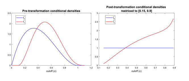
Figure 1: On the left panel, $f_{0}^{*}$, the blue curve, is the $\beta(2,3)$ pdf so that $[a_{0},b_{0}]=[0,1]$ and $f^{*}_{0}$ is not bounded away from zero. $f_{1}^{*}$, the red curve, is $\beta(3,4)+0.1$ so that $[a_{1},b_{1}]=[0.1,1.1]$. The likelihood ratio is zero below 0.1 and becomes unbounded just below 1. On the right panel, we apply the transformation $\Phi=\,$cdf of $\beta(2,3)$. $f^{*}_{0}$ is now the uniform[0,1] density so that $f_{1}^{*}$ transforms into the likelihood ratio. Assumption 4.1(iii) is satisfied over, say, $[c_{0,L},c_{0,U}]=[0.15,0.9]$ so that uniform inference about $R(t,\beta^{*})$ is possible over $[FP(c_{0,U},\beta^{*}),FP(c_{0,L},\beta^{*})]\approx[0.004,0.89]$.

Of course, Assumption 4.1 allows for scenarios in which $[FP(c_{0,U},\beta^{*}),FP(c_{0,L},\beta^{*})]=[0,1]$, i.e., uniform inference is possible along the entire ROC curve. This is the case, for example, if the “propensity score” function $P(Y=1|X=x)$ takes values from an interval $[\delta,1-\delta]$ for some $0<\delta<1/2$, which implies $supp(f_{0}^{*})=supp(f_{1}^{*})$ and that (iii) holds with $[c_{0,L},c_{0,U}]=[a_{0},b_{0}]$. More generally, Assumption 4.1(iii) allows $f^{*}_{1}(c)/f^{*}_{0}(c)$ to reach zero or explode for cutoffs $c$ outside the range $[c_{0,L},c_{1,L}]$. For example, the likelihood ratio vanishes as $c$ approaches $a_{0}$ from above whenever $a_{0}<a_{1}$. In this case the lowest index values imply $Y=0$ and the ROC curve reaches the top of the unit square for some $FP$ rate below unity. Similarly, $f^{*}_{1}(c)/f^{*}_{0}(c)$ may become unbounded as $c$ approaches $b_{0}$ from below. This can easily happen when $b_{0}<b_{1}$, i.e., the largest index values are associated exclusively with the $Y=1$ outcome. In this case the ROC curve has a positive vertical intercept at $FP=0$. Again, see Figure 1 for an example.

The next assumption is a strengthening of Assumption 3.1. These stricter conditions on the gradient vectors $\nabla_{\beta}TP(c,\beta)$ and $\nabla_{\beta}FP(c,\beta)$ also play a key role in establishing a uniform influence function representation for the sample ROC curve. Recall that $B^{*}(r)$ denote the open ball with radius $r>0$ centered on $\beta^{*}$.

Assumption 11 Let $\mathcal{C}=[a_{1},b_{1}]$. $\nabla_{\beta}TP(c,\beta)$ exits and is continuous over $\mathcal{C}\times B^{*}(r)$ for some $r>0$ with $\sup_{(c,\beta)\in\mathcal{C}\times B^{*}(r)}\|\nabla_{\beta}TP(c,\beta)\|\leq M$ for some $M>0$. The same applies to $\nabla_{\beta}FP(c,\beta)$ with $\mathcal{C}=[a_{0},b_{0}]$.

4.2 Functional limit results

Letting $c^{*}_{t}={FP}_{\beta^{*}}^{-1}(t)\in[a_{0},b_{0}]$ and $\hat{c}_{t}=\widehat{FP}_{\hat{\beta}}^{-1}(t)\in[a_{0},b_{0}]$, we start from a decomposition of $\sqrt{n}[\widehat{TP}(\hat{c}_{t},\hat{\beta})-TP(c^{*}_{t},\beta^{*})]$ similar to (7). There are two added layers of difficulty. First, functional results require uniform approximations to these terms as $t$ varies over the $[0,1]$ interval. Second, instead of being fixed, the cutoff is now estimated for any given value of $t$. The sampling variation in $\hat{c}_{t}$ contributes another non-trivial term to the asymptotic distribution.

We express the centered and scaled empirical ROC curve as the sum of three terms:

$$\sqrt{n}[\widehat{R}(t,\hat{\beta})-R(t,\beta^{*})]=\sqrt{n}[\widehat{TP}(\hat{c}_{t},\hat{\beta})-TP(c^{*}_{t},\beta^{*})]\\ =\sqrt{n}[\widehat{TP}(\hat{c}_{t},\hat{\beta})-TP(\hat{c}_{t},\hat{\beta})]+\sqrt{n}[TP(\hat{c}_{t},\hat{\beta})-TP(\hat{c}_{t},\beta^{*})]\\ +\sqrt{n}[TP(\hat{c}_{t},\beta^{*})-TP(c^{*}_{t},\beta^{*})]$$ (16)

The first term in equation (16) can be expanded similarly to the second equality in (7):

$$\sqrt{n}[\widehat{TP}(\hat{c}_{t},\hat{\beta})-TP(\hat{c}_{t},\hat{\beta})]=\sqrt{n}[\widehat{TP}(c^{*}_{t},\beta^{*})-TP(c^{*}_{t},\beta^{*})]+R_{1n}(t),$$ (17)

where $\sup_{t\in[0,1]}|R_{1n}(t)|=o_{p}(1)$. The uniform convergence of the remainder term is a consequence of the stochastic equicontinuity of the process $(c,\beta)\mapsto\sqrt{n}(\widehat{TP}(c,\beta)-TP(c,\beta))$, stated directly in Assumption 3.1, coupled with the fact that $\hat{\beta}\rightarrow_{p}\beta^{*}$ (Assumption 3.1) and $\sup_{t\in[0,1]}|\hat{c}_{t}-c^{*}_{t}|\rightarrow_{p}0$ (Lemma A.5 in Appendix A). This last result makes use of Assumption 4.1(i), which requires that the density $f_{0}^{*}$ be bounded away from zero on its compact support.

The second term in equation (16) is due to the estimation of $\beta$ and is again handled by a standard mean value expansion:

$$\sqrt{n}[TP(\hat{c}_{t},\hat{\beta})-TP(\hat{c}_{t},\beta^{*})]=\nabla_{\beta}TP(c^{*}_{t},\beta^{*})\sqrt{n}(\hat{\beta}-\beta^{*})+R_{2n}(t),$$ (18)

where $\sup_{t\in[0,1]}|R_{2n}(t)|=o_{p}(1)$. The uniformity of the approximation is ensured by Assumption 4.1, which implies that $\nabla_{\beta}TP(c,\beta^{*})$ is uniformly continuous.

Finally, the third term in (16) arises because of the need to estimate the cutoff value associated with a given false positive rate $t$; it therefore does not arise in the fixed-cutoff setting. Starting with a mean value expansion of $TP(\hat{c}_{t},\beta^{*})$ around $c^{*}_{t}$, one can write

$$\sqrt{n}[TP(\hat{c}_{t},\beta^{*})-TP(c^{*}_{t},\beta^{*})] = f_{1}^{*}(c^{*}_{t})\sqrt{n}(\hat{c}_{t}-c^{*}_{t})+R_{3n}(t)$$ (19)

$$= f_{1}^{*}(c^{*}_{t})\sqrt{n}[\widehat{FP}_{\hat{\beta}}^{-1}(t)-FP^{-1}_{\beta^{*}}(t)]+R_{3n}(t),$$

The remainder term $R_{3n}(t)$ converges in probability to zero uniformly over the interval

$$\big{\{}t:c^{*}_{t}\in[c_{0,L},c_{0,U}]\big{\}}=\big{[}FP(c_{0,U},\beta^{*}),FP(c_{0,L},\beta^{*})\big{]},$$

where $c_{0,L}$ and $c_{0,U}$ are specified in Assumption 4.1(iii). The asymptotic distribution of the process $t\mapsto\sqrt{n}[\widehat{FP}_{\hat{\beta}}^{-1}(t)-FP^{-1}_{\beta^{*}}(t)]$ can be analyzed in two steps: First, we establish an asymptotically linear representation for the “base process” $c\mapsto\sqrt{n}[\widehat{FP}(c,\hat{\beta})-FP(c,\beta^{*})]$ that holds uniformly in $c$ (and implies a mean zero Gaussian limit process). Second, we apply the functional delta method under the inverse functional $\phi(F)=F^{-1}$ to characterize the contribution of the term (19) to the asymptotic distribution of the empirical ROC curve.

Lemma 1 summarizes and completes the development of the approximations presented in equations (17), (18) and (19).

Lemma 1

Suppose that Assumptions 2.2, 3.1, 3.1, 4.1 and 4.1 are satisfied. Then:

(i) $\sup_{t\in[0,1]}R_{1n}(t)=o_{p}(1)$;

(ii) $\sup_{t\in[0,1]}R_{2n}(t)=o_{p}(1)$;

(iii) $\sup_{t\in T}R_{3n}(t)=o_{p}(1)$, where $T=\big{[}FP(c_{0,U},\beta^{*}),FP(c_{0,L},\beta^{*})\big{]}$;

(iv) $\widehat{FP}(c,\hat{\beta})$ admits asymptotically linear representation that holds uniformly in $c$:

$$\sqrt{n}\big{(}\widehat{FP}(c,\hat{\beta})-FP(c,\beta^{*})\big{)}=\frac{1}{\sqrt{n}}\sum_{i=1}^{n}\psi_{FP}(Y_{i},X_{i},c,\beta^{*})+R_{4n}(t),$$ (20)

where $\sup_{c_{\in}[a_{0},b_{0}]}R_{4n}(c)=o_{p}(1)$;

(v) and, by the functional delta method,

$$\sqrt{n}[\widehat{FP}_{\hat{\beta}}^{-1}(t)-FP^{-1}_{\beta^{*}}(t)]=-\frac{1}{f_{0}^{*}(c^{*}_{t})}\sqrt{n}[\widehat{FP}(c^{*}_{t},\hat{\beta})-FP(c^{*}_{t},\beta^{*})]+R_{5n}(t),$$ (21)

where $\sup_{t\in(0,1)}|R_{5n}(t)|=o_{p}(1)$.

Remarks

1. The proof of Lemma 1 is provided in Appendix B; it simply adds some technical details to the arguments outlined in the main text.

2. The fact that $f^{*}_{0}(c)$ is bounded away from zero (Assumption 4.1(i)) plays a critical role in ensuring that the remainder term $R_{5n}(t)$ associated with the delta method converges to zero uniformly over the entire $[0,1]$ interval.

Combining equations (16) through (21) with the influence function representations of $\sqrt{n}[\widehat{TP}(c,\beta^{*})-TP(c,\beta^{*})]$ and $\sqrt{n}(\hat{\beta}-\beta^{*})$ yields the following proposition, which is the central result of the paper.

Proposition 6

Suppose that Assumptions 2.2, 3.1, 3.1, 4.1 and 4.1 are satisfied. Define

$$\psi_{R}(y,x,t,\beta^{*})=\psi_{TP}(y,x,c^{*}_{t},\beta^{*})-\frac{f_{1}^{*}(c^{*}_{t})}{f_{0}^{*}(c^{*}_{t})}\psi_{FP}(y,x,c^{*}_{t},\beta^{*}),$$

where $c^{*}_{t}=FP^{-1}_{\beta^{*}}(t)$. Then:

(i) The empirical ROC curve admits an asymptotically linear representation that holds uniformly over $T=\big{[}FP(c_{0,U},\beta^{*}),FP(c_{0,L},\beta^{*})\big{]}$:

$$\sup_{t\in T}\Big{|}\sqrt{n} \big{(}\widehat{R}(t,\hat{\beta})-R(t,\beta^{*})\big{)}-\frac{1}{\sqrt{n}}\sum_{i=1}^{n}\psi_{R}(Y_{i},X_{i},t,\beta^{*})\Big{|}=o_{p}(1),$$ (22)

where $c_{0,L}$ and $c_{0,U}$ are chosen in accordance with Assumption 4.1(iii), i.e., $f_{1}^{*}/f_{0}^{*}$ is continuous and bounded away from zero on $[c_{0,L},c_{0,U}]$ .

(ii) The process $t\mapsto\frac{1}{\sqrt{n}}\sum_{i=1}^{n}\psi_{R}(Y_{i},X_{i},t,\beta^{*})$ is stochastically equicontinuous over $T$.

(iii) Therefore,

$$\sqrt{n}(\widehat{R}_{n}(t,\hat{\beta})-{R}(t,\beta^{*}))\Rightarrow\Psi_{h_{R}}(t)\text{ in the space $L^{\infty}(T)$},$$

where “$\Rightarrow$” denotes weak convergence, $L^{\infty}(T)$ is the space of bounded functions over $T$, and $\Psi_{h_{R}}(\cdot)$ is a zero mean Gaussian process defined on $T$ with covariance kernel $h_{R}(t_{1},t_{2})=E[\psi_{R}(Y,X,t_{1},\beta^{*})\psi_{R}(Y,X,t_{2},\beta^{*})]$.

Remarks

1. The precise notion of weak convergence employed in part (iii) is given by Definition 1.3.3 of van der Vaart and Wellner (1996).

2. Given the arguments leading up to Proposition 6, the proof of part (i) is practically complete (technically, it still requires showing that the influence function representation of $\sqrt{n}[\widehat{TP}(c,\beta^{*})-TP(c,\beta^{*})]$ holds uniformly in $c$, but this is essentially covered by Lemma 1(iv)). The proof of Part (ii) relies on Assumptions 3.1, 4.1 and 4.1. Part (iii) follows immediately from parts (i) and (ii). Details are presented in Appendix B.

4.3 Simulating the asymptotic distribution of the ROC curve

In order to employ Proposition 6 for statistical inference, we need a method to approximate $\Psi_{h_{R}}(t)$, the distributional limit of the process $\sqrt{n}(\widehat{R}_{n}(t,\beta^{*})-{R}(t,\beta^{*}))$. To this end, offer two methods: the weighted bootstrap as in Ma and Korosok (2005) and the multiplier bootstrap as in Hsu (2016).

We first present the discussion of the weighted bootstrap. Define $\widehat{TP}^{w}(c,\hat{\beta}^{w})$ and $\widehat{FP}^{w}(c,\hat{\beta}^{w})$ precisely as in Section 3.4 and let $\hat{c}^{w}_{t}=\big{(}\widehat{FP}^{w}_{\hat{\beta}^{w}}\big{)}^{-1}(t)$. We can then construct the weighted ROC curve and its estimated limit process as $\widehat{R}^{w}_{n}(t,\hat{\beta}^{w})=\widehat{TP}^{w}(\hat{c}^{w}_{t},\hat{\beta}^{w})$ and $\widehat{\Psi}^{w}_{R,n}(t)=\sqrt{n}(\widehat{R}^{w}_{n}(t,\hat{\beta}^{w})-\widehat{R}_{n}(t,\hat{\beta}))$.

Proposition 7

Suppose that 2.2-3.1, and 3.4-4.1 are satisfied. Then, conditional on the sample path of the data, $\widehat{\Psi}^{w}_{R,n}(\cdot)\Rightarrow\Psi_{h_{R,2}}(\cdot)$ in the space $L^{\infty}(T)$ with probability approaching one.

Under the conditions of Proposition 6, one can apply the arguments in Theorem 2 of Ma and Kosorok (2005) to show that $\widehat{\Psi}^{w}_{R,n}(t)$ also approximates the distribution of $\Psi_{h_{R,2}}(t)$ in the sense of Proposition 8. That is, conditional on the sample path of the data, $\widehat{\Psi}^{w}_{R,n}(t)\Rightarrow\Psi_{h_{R,2}}(t)$ with probability approaching one.

We now turn to the discussion of the multiplier bootstrap method that is based on the conditional multiplier central limit theorem (see, e.g., van der Vaart and Wellner 1996, Section 2.9). The method requires consistent estimation of the components of the influence function $\psi_{R}$, uniformly in $t$. However, this estimation needs to be performed only once, over the original data set, given that the method does not rely on successive resampling and reestimation.

Let $\widehat{\psi}_{\beta}(y,x,\hat{\beta})$ denote the estimated influence function of $\hat{\beta}$, where we replace any unknown parameters or functions within $\psi_{\beta}$ with consistent estimators (note that this function does not depend on $t$). We make the general assumption that the asymptotic variance-covariance matrix of $\hat{\beta}$ is consistently estimable using $\widehat{\psi}_{\beta}$ and the sample analog principle:

Assumption 12 Let $V=E[{\psi}_{\beta}(Y,X,\beta^{*}){\psi}_{\beta}(Y,X,\beta^{*})^{\prime}]$. Then:

$$\widehat{V}_{n}=n^{-1}\sum_{i=1}^{n}\widehat{\psi}_{\beta}(Y_{i},X_{i},\hat{\beta}_{n})\widehat{\psi}_{\beta}(Y_{i},X_{i},\hat{\beta}_{n})^{\prime}\stackrel{{\scriptstyle p}}{{\rightarrow}}V.$$

Let $\mathcal{C}=[c_{0,L},c_{0,U}]$. We further assume that there exist uniformly consistent estimators for $\nabla_{\beta}FP(c,\beta^{*})$, $\nabla_{\beta}TP(c,\beta^{*})$ and $f_{1}^{*}(c)/f_{0}^{*}(c)$ on $\mathcal{C}$. Here we state the existence of these estimators as a high level assumption and provide concrete implementations and additional assumptions in Appendix C.

Assumption 13 The estimators $\nabla_{\beta}\widehat{FP}(c,\hat{\beta}_{n})$, $\nabla_{\beta}\widehat{TP}(c,\hat{\beta}_{n})$, and $\hat{f}_{1}(c)/\hat{f}_{0}(c)$ are Lipschitz continuous in $c$ on $\mathcal{C}$ which is compact and satisfy

$$\sup_{c\in\mathcal{C}}\|\nabla_{\beta}\widehat{FP}(c,\hat{\beta}_{n})-\nabla_{\beta}FP(c,\beta^{*})\|=o_{p}(1),$$

$$\sup_{c\in\mathcal{C}}\|\nabla_{\beta}\widehat{TP}(c,\hat{\beta}_{n})-\nabla_{\beta}TP(c,\beta^{*})\|=o_{p}(1),$$

$$\sup_{c\in\mathcal{C}}\left|\frac{\hat{f}_{1}(c)}{\hat{f}_{0}(c)}-\frac{f_{1}(c)}{f_{0}(c)}\right|=o_{p}(1).$$

In addition, the estimator $\hat{c}_{t}$ is uniformly consistent for $c_{t}$ for $t\in T$.

We now present the multiplier bootstrap. Let $U_{1},\ldots,U_{n}$ be i.i.d. random variables independent of the data with moments $E[U]=0$, $E[U^{2}]=1$, and $E|U|^{2+\delta_{u}}<\infty$ for some $\delta_{u}>0$. For $t\in[0,1]$, we define the simulated stochastic process $\widehat{\Psi}^{u}_{R,n}(t)$ as

$$\widehat{\Psi}^{u}_{R,n}(t)=\frac{1}{\sqrt{n}}\sum^{n}_{i=1}U_{i}\cdot\widehat{\psi}_{R}(Y_{i},X_{i},t,\hat{\beta}),$$ (23)

where

$$\hat{\psi}_{R}(y,x,t,\beta)=\hat{\psi}_{TP}(y,x,\hat{c}_{t},\beta)-\frac{\hat{f}_{1}(\hat{c}_{t})}{\hat{f}_{0}(\hat{c}_{t})}\hat{\psi}_{FP}(y,x,\hat{c}_{t},\beta),$$

$$\hat{\psi}_{TP}(y,x,c,\beta)=\frac{y}{\hat{\pi}}\Big{(}1[G(x,\beta)>c]-\widehat{TP}(c,\beta)\Big{)}+\nabla_{\beta}\widehat{TP}(c,\beta)\hat{\psi}_{\beta}(y,x,\beta),$$

$$\hat{\psi}_{FP}(y,x,c,\beta)=\frac{1-y}{1-\hat{\pi}}\Big{(}1[G(x,\beta)>c]-\widehat{FP}(c,\beta)\Big{)}+\nabla_{\beta}\widehat{FP}(c,\beta)\hat{\psi}_{\beta}(y,x,\beta),$$

$$\hat{\pi}=\frac{1}{n}\sum_{i=1}^{n}Y_{i}.$$

The next result shows that the distribution of the simulated process $\widehat{\Psi}^{u}_{R,n}(t)$ approximates that of the true limiting process $\Psi_{h_{R,2}}(t)$ in large samples.

Proposition 8

Suppose that Assumptions 2.2-3.1 and 4.1-4.3 are satisfied. Then, conditional on the sample path of the data, $\widehat{\Psi}^{u}_{R,n}(\cdot)\Rightarrow\Psi_{h_{R,2}}(\cdot)$ in the space $L^{\infty}(T)$ with probability approaching one.

The weighted bootstrap has the advantage that it does not require explicit estimation of this function, but it is computationally somewhat more costly. On the other hand, the proof of weighted bootstrap is less involved because the multiplier method relies heavily on Assumption 4.3, i.e., the availability of uniformly consistent estimators for the components of $\psi_{R}$. To obtain estimators satisfy Assumption 4.3 additional assumptions are needed and in Appendix C, we provide estimators and additional assumptions so that Assumption 4.3 can be satisfied and we can apply multiplier method.

5 Applications to various inference problems

In this section, we provide some examples that we can apply the results in Section 4.

5.1 Uniform confidence bands

Let $\widehat{\sigma}^{2}_{t}$ denote a uniform consistent estimator for ${\sigma}^{2}_{t}$, the asymptotic variance of $\sqrt{n}(\widehat{R}_{n}(t,\hat{\beta})-{R}(t,\beta^{*}))$ for $t\in T$. Later we will provide two estimators based on weighted bootstrap method and analytic results. Let $\widehat{\sigma}_{t,\epsilon}=\max\{\widehat{\sigma}_{t},\epsilon\}$ in which $\epsilon>0$ is a fixed and small number. We are interested in a standardized version of confidence bands and by truncating $\widehat{\sigma}_{t}$ by $\epsilon$, we can make sure that we will not divide something close to zero when $t$ is close to 0 or 1.

For a nominal significance level $\alpha$ and for $\tau_{\ell},\tau_{u}\in T$ with $\tau_{\ell}\leq\tau_{u}$, let $\widehat{C}^{\text{1-sided}}_{\alpha}$ and $\widehat{C}^{\text{2-sided}}_{\alpha}$ respectively denote the one- and two-sided critical values that satisfy

$$\widehat{C}^{\text{1-sided}}_{\alpha} =\inf_{a\in R}\left\{P\left(\sup_{t\in[\tau_{\ell},\tau_{u}]}\frac{\widehat{\Psi}^{w}_{R,n}(t)}{\widehat{\sigma}_{t,\epsilon}}\leq a\right)\geq 1-\alpha\right\},$$ (24)

$$\widehat{C}^{\text{2-sided}}_{\alpha} =\inf_{a\in R}\left\{P\left(\sup_{t\in[\tau_{\ell},\tau_{u}]}\frac{|\widehat{\Psi}^{w}_{R,n}(t)|}{\widehat{\sigma}_{t,\epsilon}}\leq a\right)\geq 1-\alpha\right\}.$$ (25)

Here, $\widehat{C}^{\text{1-sided}}_{\alpha}$ and $\widehat{C}^{\text{2-sided}}_{\alpha}$ are, respectively, the $(1-\alpha)$th quantile of $\sup_{t\in[\tau_{\ell},\tau_{u}]}\widehat{\Psi}^{w}_{R,n}(t)\big{/}\widehat{\sigma}_{t,\epsilon}$ and $(1-\alpha)$th quantile of $\sup_{t\in[\tau_{\ell},\tau_{u}]}\big{|}\widehat{\Psi}^{w}_{R,n}(t)\big{/}\widehat{\sigma}_{t,\epsilon}\big{|}$. Note that one can replace $\widehat{\Psi}^{w}_{R,n}(t)$ with $\widehat{\Psi}^{u}_{R,n}(t)$ to construct $\widehat{C}^{\text{1-sided}}_{\alpha}$ and $\widehat{C}^{\text{2-sided}}_{\alpha}$ as well.

Once the critical values are constructed, we can also obtain one- and two-sided uniform confidence bands for ${R}(t,\beta^{*})$ over $[\tau_{\ell},\tau_{u}]$. Specifically, the one-sided $(1-\alpha)$ uniform confidence band is given by

$$\left(\widehat{R}_{n}(t,\hat{\beta})-\widehat{C}^{\text{1-sided}}_{\alpha}\frac{\widehat{\sigma}_{t,\epsilon}}{\sqrt{n}},\quad+\infty\right),\quad\tau\in[\tau_{\ell},\tau_{u}]$$ (26)

and the two-sided $(1-\alpha)$ uniform confidence band is

$$\left(\widehat{R}_{n}(t,\hat{\beta})-\widehat{C}^{\text{2-sided}}_{\alpha}\frac{\widehat{\sigma}_{t,\epsilon}}{\sqrt{n}},\quad\widehat{R}_{n}(t,\hat{\beta})+\widehat{C}^{\text{2-sided}}_{\alpha}\frac{\widehat{\sigma}_{t,\epsilon}}{\sqrt{n}}\right),\quad\tau\in[\tau_{\ell},\tau_{u}].$$ (27)

Implementation of Uniform Confidence Bands

We now provide a step-by-step implementation for constructing uniform confidence bands.

1. Obtain $\widehat{R}_{n}(t,\hat{\beta})$ from Section 4 and $\widehat{\sigma}_{t,\epsilon}$ from Section 5.1 with $t\in\{\tau_{\ell},\tau_{\ell}+0.01,\dotsc,\tau_{u}\}$.

2. Draw i.i.d. pseudo random variables $\{W_{1},\dotsc,W_{n}\}$ where $W_{i}$’s are normal distributions with mean and variance equal to one $B$ times for, say, $B=1000$. For each repetition $b=1,\dotsc,B$, calculate the simulated process $\widehat{\Psi}^{w}_{R,n}(t)$ according to (23).

3. For the one-sided case, store the maximum value of ${\widehat{\Psi}^{w}_{R,n}(t)}\big{/}{\widehat{\sigma}_{t,\epsilon}}$ over the grid of $t$ values set up in Step 1; that is, let $M_{b}=\max_{t\in\{\tau_{\ell},\tau_{\ell}+0.01,\dotsc,\tau_{u}\}}{\widehat{\Psi}^{w}_{R,n}(t)}\big{/}{\widehat{\sigma}_{t,\epsilon}}$ for $b=1,\dotsc,B$.

4. Rank the $M_{b}$ values in an ascending order so that $M_{(1)}\leq\dotsc\leq M_{(B)}$. Next, define $M_{(\lfloor(1-\alpha)B\rfloor)}$ as the critical value $\widehat{C}^{\text{1-sided}}_{\alpha}$, where $\lfloor a\rfloor$ is the floor function returning the largest integer not greater than $a$. The one-sided $(1-\alpha)$ uniform confidence bands for $\{{R}(t,\beta^{*}):t\in[\tau_{\ell},\tau_{u}]\}$ are given by (26).

5. For the two-sided case, simply replace ${\widehat{\Psi}^{w}_{R,n}(t)}\big{/}{\widehat{\sigma}_{t,\epsilon}}$ in Step 3 with $\big{|}{\widehat{\Psi}^{w}_{R,n}(t)}\big{|}\big{/}{\widehat{\sigma}_{t,\epsilon}}$ and repeat Step 4 for the critical value $\widehat{C}^{\text{2-sided}}_{\alpha}$. The two-sided $(1-\alpha)$ uniform confidence band for $\{{R}(t,\beta^{*}):t\in[\tau_{\ell},\tau_{u}]\}$ is given by (27).

Uniformly consistent estimators for ${\sigma}^{2}_{t}$
We consider two estimators here. First estimator is based on weighted bootstrap that is similar to Remark 2 after Proposition 5. Let $\widehat{\Psi}^{w}_{R,n}(t)$ denote the ROC estimate from the $w$th bootstrap cycle, $w=1,\ldots,\mathcal{W}$. Then one can estimate ${\sigma}^{2}_{t}$ by

$$\widehat{\sigma}^{2}_{t}=\frac{n}{\mathcal{W}}\sum_{w=1}^{\mathcal{W}}\big{(}\widehat{R}^{w}_{n}(t,\hat{\beta}^{w})-\overline{\widehat{R}}^{w}_{n}(t,\hat{\beta}^{w})\big{)}\big{(}\widehat{R}^{w}_{n}(t,\hat{\beta}^{w})-\overline{\widehat{R}}^{w}_{n}(t,\hat{\beta}^{w})\big{)}^{\prime},\text{ where}$$

$$\overline{\widehat{R}}^{w}_{n}(t,\hat{\beta}^{w})=\frac{1}{\mathcal{W}}\sum_{w=1}^{\mathcal{W}}\widehat{R}^{w}_{n}(t,\hat{\beta}^{w}).$$

We have that conditional on sample path with probability approaching one,

$$\widehat{\sigma}^{2}_{t}\stackrel{{\scriptstyle p}}{{\rightarrow}}_{w}\frac{1}{n}\sum_{i=1}^{n}\psi^{2}_{R}(Y_{i},X_{i},t,\beta^{*})+o_{p}(1),$$

where $\stackrel{{\scriptstyle p}}{{\rightarrow}}_{w}$ denotes probability limit under the law of the $W_{i}$’s. It follows that uniformly over $t\in[t_{\ell},t_{u}]$,

$$\lim_{\mathcal{W}\rightarrow\infty}\widehat{\sigma}^{2}_{t}\stackrel{{\scriptstyle p}}{{\rightarrow}}{\sigma}^{2}_{t}.$$

The second estimator is based on analytic results. Recall that $\widehat{\psi}_{R}(Y_{i},X_{i},t,\hat{\beta})$ is the estimated influence function for $\widehat{R}_{n}(t,\hat{\beta})$ used in the multiplier bootstrap method. A uniformly consistent estimator for ${\sigma}^{2}_{t}$ is given by

$$\widehat{\sigma}^{2}_{t}=\frac{1}{n}\sum_{i=1}^{n}\widehat{\psi}^{2}_{R}(Y_{i},X_{i},t,\hat{\beta})$$

and this is shown in the proof of 8.

5.2 ROC dominance test

For two predictive index models $G_{1}(X,\beta_{1})$ and $G_{2}(X,\beta_{2})$, we may want to test whether $G_{1}$ has strictly better predictive power than $G_{2}$ in the sense that the ROC curve associated with $G_{1}$ dominates the ROC curve associated with $G_{2}$. What domination means is that for any given false positive rate $G_{1}$ delivers a higher true positive rate, i.e., the ROC curve for $G_{1}$ always lies above the ROC curve for $G_{2}$. Any decision maker, regardless of their loss function and their optimal cutoff, would then prefer model $G_{1}$ over $G_{2}$.

Let $R_{1}(t,\beta_{1}^{*})$ and $R_{2}(t,\beta_{2}^{*})$ denote the ROC curves associated with $G_{1}$ and $G_{2}$, respectively. The hypotheses that $R_{1}(t,\beta_{1}^{*})$ dominates $R_{2}(t,\beta_{2}^{*})$ can be formally stated as

$$H_{0}:R_{2}(t,\beta_{2}^{*})\leq R_{1}(t,\beta_{1}^{*})~{}~{}\text{ for all $t\in[0,1]$},$$

$$H_{1}:R_{2}(t,\beta_{2}^{*})>R_{1}(t,\beta_{1}^{*})~{}~{}\text{ for some $t\in[0,1]$}.$$ (28)

Our test for ROC dominance is similar to the test for first order stochastic dominance in Barrett and Donald (2003) and Donald and Hsu (2016) except that we need to consider the estimation effect of $\hat{\beta}$ as in Linton, Massoumi and Whang (2005) and Linton, Song and Whang (2010).

Let $\widehat{R}_{j,n}(t,\hat{\beta}_{j})$ be the estimators for $R_{j}(t,\beta_{j}^{*})$ for $j=1,2$. Define $\psi_{j,R}(Y_{i},X_{i},t,\beta_{1}^{*})$ for $j=1$ and 2 as above. Let $\widehat{\sigma}^{2}_{RD}(t)$ denote a uniform consistent estimator for ${\sigma}^{2}_{RD}(t)$, the asymptotic variance of $\sqrt{n}(\widehat{R}_{2,n}(t,\hat{\beta}_{2})-\widehat{R}_{1,n}(t,\hat{\beta}_{1})-{R}_{2}(t,{\beta}^{*}_{2})-{R}_{1}(t,{\beta}^{*}_{1}))$. Let $\widehat{\sigma}_{RD,\epsilon}(t)=\max\{\widehat{\sigma}_{RD}(t),\epsilon\}$ in which $\epsilon>0$ is a fixed and small number. Uniform consistent estimator $\widehat{\sigma}^{2}_{RD}(t)$ can be obtained similar to $\widehat{\sigma}^{2}_{t}$ in Section 5.1, so we omit the details.

We define the test statistic as $\widehat{S}_{n}=\sqrt{n}\sup_{t\in[0,1]}(\widehat{R}_{2,n}(t,\hat{\beta}_{2})-\widehat{R}_{1,n}(t,\hat{\beta}_{1}))/\widehat{\sigma}_{RD,\epsilon}(t)$. Define the weighted bootstrap process $\Psi^{w}_{RD,n}(t)$ as $\widehat{\Psi}^{w}_{R,n}(t)=\sqrt{n}\big{(}\widehat{R}^{w}_{2,n}(t,\hat{\beta}^{w}_{2})-\widehat{R}^{w}_{1,n}(t,\hat{\beta}^{w}_{1})-(\widehat{R}_{2,n}(t,\hat{\beta}_{2})-\widehat{R}_{1,n}(t,\hat{\beta}_{1}))\big{)}$ and define the multiplier bootstrap process $\Psi^{u}_{RD,n}(t)$ as

$$\widehat{\Psi}^{u}_{RD,n}(t)=\frac{1}{\sqrt{n}}\sum_{i=1}^{n}U_{i}\cdot(\widehat{\psi}_{2,R}(Y_{i},X_{i},t,\hat{\beta}_{2})-\widehat{\psi}_{1,R}(Y_{i},X_{i},t,\hat{\beta}_{1})).$$

Under the least favorable configuration, we define the weighted bootstrap critical value as

$$\hat{c}_{n}=\sup\Big{\{}c\big{|}P^{w}\Big{(}\sqrt{n}\sup_{t\in[0,1]}\frac{\widehat{\Psi}^{w}_{RD,n}(t)}{\widehat{\sigma}_{RD,\epsilon}(t)}\leq c\Big{)}\leq 1-\alpha\Big{\}},$$ (29)

with significance level $\alpha$. The decision rule is

Reject $$H_{0} \widehat{S}_{n}>\hat{c}_{n}$$ if . (30)

Then one can use $\widehat{\Psi}^{u}_{RD,n}(t)$ to construct critical value $\hat{c}_{n}$ as well.

Similar to the stochastic dominance test literature, we can show that under the null hypothesis the asymptotic size of a test with decision rule defined in (30) is less than or equal to $\alpha$. That is, we can control the asymptotic size of our ROC dominance test well. Also, under the fixed alternative, we have the test statistic converging to positive infinity and the critical value converging to a finite number, so the test is consistent. Our test is based on least favorable configuration, so it is conservative in that the asymptotic size is strictly smaller than $\alpha$ unless $R_{2}(t,\beta_{2}^{*})=R_{1}(t,\beta_{1}^{*})$ for all $t\in[0,1]$. One can improve the power of our test by using the recentering method in Hansen (2005), Donald and Hsu (201) which is similar to the generalized moment selection method in Andrews and Soreas (2010), and Andrews and Shi (2013), and the contact set approach in Linton, Song and Whang (2010). In this paper, we do not adopt this approach but the extension is straightforward.

5.3 Comparing AUCs

Recall that AUC is defined as the integral of ROC curve from 0 to one. Following Section 5.2, let $R_{1}(t,\beta_{1}^{*})$ and $R_{2}(t,\beta_{2}^{*})$ denote the ROC curves for two predictive index models $G_{1}(X,\beta_{1})$ and $G_{2}(X,\beta_{2})$. Let $AUC_{j}=\int_{0}^{1}R_{j}(t,\beta_{j}^{*})dt$ and its estimator be $\widehat{AUC}_{j}=\int_{0}^{1}\widehat{R}_{j,n}(t,\hat{\beta}_{j})dt$ for $j=1$ and 2. Then it is true that

$$\sqrt{n}(\widehat{AUC}_{2}-\widehat{AUC}_{1})=\frac{1}{\sqrt{n}}\sum_{i=1}^{n}\int_{0}^{1}({\psi}_{2,R}(Y_{i},X_{i},t,\beta^{*}_{2})-{\psi}_{1,R}(Y_{i},X_{i},t,{\beta}^{*}_{1})dt+o_{p}(1)$$

and

$$\sqrt{n}(\widehat{AUC}_{2}-\widehat{AUC}_{1}){\rightarrow}_{d}N[0,\mathcal{V}_{a}],$$

$$\mathcal{V}_{a}=E[\big{(}\int_{0}^{1}{\psi}_{2,R}(Y,X,t,\beta^{*}_{2})-{\psi}_{1,R}(Y,X,t,{\beta}^{*}_{1})dt\big{)}^{2}].$$

To make inference, one can use a weighted bootstrap method to approximate the limiting distribution of $N[0,\mathcal{V}_{a}]$ or one can estimate $\mathcal{V}_{a}$ analytically by

$$\widehat{\mathcal{V}}_{a}=\frac{1}{n}\sum_{i=1}^{n}\Big{(}\int_{0}^{1}(\widehat{\psi}_{2,R}(Y_{i},X_{i},t,\hat{\beta}_{2})-\widehat{\psi}_{1,R}(Y_{i},X_{i},t,\hat{\beta}_{1}))dt\Big{)}^{2}.$$

For brevity, we omit the details here.

Remark
Suppose that $G(X,\beta)$ is a correct specification for the propensity score function, $P(Y=1|X)$, in that there exists $\beta^{*}$ such that $G(X,\beta^{*})=P(Y=1|X)$ a.s. Then the estimation effect of $\beta^{*}$ on the distribution of AUC is negligible. It is then true that when two predictive predictive index models, $G_{1}(X,\beta_{1})$ and $G_{2}(X,\beta_{2})$, are both correctly specified for $P(Y=1|X)$, we have $\mathcal{V}_{a}=0$, i.e., the limiting distribution of $\sqrt{n}(\widehat{AUC}_{2}-\widehat{AUC}_{1})$ is degenerate.

6 Simulations: the relevance of the estimation effect

We now present a small Monte Carlo simulation to illustrate the theoretical discussion of the estimation effect and the pointwise asymptotic results in Section 3. The data generating process (DGP) is specified as follows. Let $X=(X_{1},X_{2},X_{3})^{\prime}$ be a $3\times 1$ vector of predictors and $\tilde{X}=(1,X^{\prime})^{\prime}$. The components of $X$ are either independent $N(0,1)$ or unif$[-.5,1.5]$ variables. The outcomes $Y$ are generated according to the conditional probability function

$$p(X)=G(X,\beta^{\circ})=G(\tilde{X}^{\prime}\beta^{\circ})\text{ with }\beta^{\circ}=(0,0.5,0.25,1)^{\prime}\text{ and }G\in\{\text{logit},\text{cauchit}\}.$$

In the majority of the exercises we use a logistic link in the DGP (so that the logit first stage is correctly specified), but we also conduct some simulations with a cauchit link (so that the logit first stage is mildly misspecified).

Given a sample of observations and a cutoff $c$, we construct nominally 90% confidence intervals for TP$(c,\beta^{\circ})$ and TP$(c,\beta^{\circ})-FP(c,\beta^{\circ})$ in three different ways: (i) using the true predictive index $p(X)=G(\tilde{X}^{\prime}\beta^{\circ})$ with the conventional limit distributions (4) and (5); (ii) using the estimated predictive index $\Lambda(\tilde{X}^{\prime}\hat{\beta})$ with the conventional limit distributions (so that the estimation effect is ignored); (iii) using the estimated predictive index $\Lambda(\tilde{X}^{\prime}\hat{\beta})$ with the corrected limit distribution (10). We simulate 10,000 samples and compute the actual coverage probability of these intervals.

Table 1: Illustration of the estimation effect: actual coverage probabilities

	Nominal 90% CIs for TP				Nominal 90% CIs for TP-FP
	True	Conventional		Corrected	True	Conventional		Corrected
$c$	value	$G(\tilde{X}^{\prime}\beta^{\circ})$	$\Lambda(\tilde{X}^{\prime}\hat{\beta})$	$\Lambda(\tilde{X}^{\prime}\hat{\beta})$	value	$G(\tilde{X}^{\prime}\beta^{\circ})$	$\Lambda(\tilde{X}^{\prime}\hat{\beta})$	$\Lambda(\tilde{X}^{\prime}\hat{\beta})$
	(A) $n=200$, $X_{1},X_{2},X_{3}\sim$iid $N(0,1)$
0.2	0.970	0.794	0.793	0.885	0.166	0.897	0.628	0.850
0.33	0.884	0.887	0.856	0.892	0.313	0.893	0.778	0.885
0.5	0.694	0.894	0.768	0.890	0.388	0.896	0.889	0.896
0.67	0.429	0.894	0.620	0.876	0.313	0.897	0.769	0.878
0.8	0.196	0.895	0.533	0.847	0.166	0.894	0.615	0.842
	(B) $n=500$, $X_{1},X_{2},X_{3}\sim$iid $N(0,1)$
0.2	0.970	0.861	0.843	0.893	0.166	0.905	0.625	0.862
0.33	0.884	0.895	0.861	0.891	0.313	0.903	0.779	0.888
0.5	0.694	0.892	0.766	0.891	0.388	0.901	0.896	0.899
0.67	0.429	0.897	0.618	0.886	0.313	0.900	0.773	0.886
0.8	0.196	0.895	0.531	0.862	0.166	0.895	0.627	0.864
	(C) $n=2500$, $X_{1},X_{2},X_{3}\sim$iid $N(0,1)$
0.2	0.970	0.893	0.857	0.901	0.166	0.902	0.630	0.885
0.33	0.884	0.898	0.863	0.899	0.313	0.899	0.779	0.899
0.5	0.694	0.899	0.779	0.902	0.388	0.901	0.902	0.899
0.67	0.429	0.898	0.633	0.896	0.313	0.894	0.776	0.896
0.8	0.196	0.895	0.545	0.881	0.166	0.898	0.630	0.885
	(D) $n=500$, $X_{1},X_{2},X_{3}\sim$unif $[-0.5,1.5]$
0.5	0.934	0.889	0.515	0.876	0.117	0.888	0.628	0.855
0.67	0.671	0.897	0.595	0.904	0.257	0.894	0.897	0.926
0.8	0.304	0.899	0.378	0.862	0.182	0.894	0.675	0.899
	(E) $n=500$, $X_{1},X_{2},X_{3}\sim$iid $N(0,1)$, $G$=cauchit
0.2	0.963	0.878	0.841	0.879	0.157	0.899	0.602	0.862
0.33	0.862	0.902	0.626	0.657	0.339	0.898	0.701	0.858
0.5	0.702	0.898	0.769	0.898	0.404	0.896	0.890	0.895
0.67	0.476	0.901	0.494	0.814	0.339	0.903	0.701	0.857
0.8	0.194	0.895	0.523	0.861	0.157	0.899	0.601	0.858

Note: $c$ is the cutoff; “True value” is the true value of $TP(c,\beta^{\circ})$ and $TP(c,\beta^{\circ})$-$FP(c,\beta^{\circ})$. All other numbers in the table are actual coverage probabilities. $G(\tilde{X}^{\prime}\beta^{\circ})$ means using the true value of $\mathbb{P}(Y=1|X)$ as the predictive index; $\Lambda(\tilde{X}^{\prime}\hat{\beta})$ means pre-estimating the predictive index by a logit regression of $Y$ on $\tilde{X}=(1,X^{\prime})^{\prime}$. The columns labeled “Conventional” report CIs based on the limit distributions (4) and (5). The columns labeled “Corrected” report CIs based on (10), which accounts for the pre-estimation effect.

Table 1 reports the results from this exercise for $c\in\{0.2,0.33,0.5,0.67,0.8\}$ and $n\in\{200,500,5000\}$. The first message is that failing to account for the pre-estimation effect can cause substantial distortions in the coverage probability of the conventional CIs. In panels (A) through (D) the estimation effect can be seen by comparing the columns titled “Conventional $G(\tilde{X}^{\prime}\beta^{\circ})$” and “Conventional $\Lambda(\tilde{X}^{\prime}\hat{\beta})$.” In the former case there is no estimation effect and any deviation from the nominal confidence level of 90% is a small sample phenomenon. Over the various cases, the estimation effect ranges from essentially zero to as large as a 30 to 40 percentage point difference in coverage probability. In panel (E), the comparison between the same two columns includes the estimation effect as well as some “bias” due to the fact that the first stage logit regression is misspecified.

The theory presented in Section 3.2 gives insight into why the estimation effect is negligible in some cases. In particular, consider the parameter $TP-FP$ on panels (A) through (C) with $c=0.5$. As the predictors are independent standard normal variables and there is no constant in the DGP, the symmetry of the logistic cdf gives $\pi=\mathbb{P}(Y=1)=0.5$. Therefore, when $c=0.5$, $TP-FP$ is a scalar multiple of $(1-c)\pi TP-c(1-\pi)FP$. As explained in footnote 10, inference about this particular linear combination is not impacted by the pre-estimation effect. This is clearly reflected in the estimation results. By contrast, in panel (D) the predictor distribution is not symmetric around zero, so $\pi\neq 0.5$, and the estimation effect is indeed present for $TP-FP$ even when $c=0.5$.

The second main message is that the proposed analytical correction works well in virtually all the cases considered here. This includes panel (A), where the sample size is small, and panel (E), where the first stage logit model is misspecified. Not surprisingly, under misspecification the corrected CI can also fall somewhat short of the 90% confidence level, but it still represents a large improvement over conventional inference.

7 Conclusions

We provided both pointwise and uniform asymptotic results that describe the distribution of an empirical ROC curve based on a pre-estimated index. The core theory is complete. Ongoing work consists of: (i) developing appropriate test procedures when the first stage models are nested and the ROC influence functions are the same under the null; (ii) additional simulations that illustrate the small sample performance of the uniform asymptotic results, the practical use of the tests, and the power gains afforded by in-sample inference.

References

• Abadie, A. and G.W. Imbens (2016): “Matching on the Estimated Propensity Score”. Econometrica, 84: 781-807.

  Andrews, D.W.K. (1994): “Empirical Process Methods in Econometrics,” in Handbook of Econometrics, vol. IV, eds. R.F. Engle and D.L. McFadden, Elsevier.

  Andrews, D. W. K. and G. Soares (2010): “Inference for Parameters Defined by Moment Inequalities Using Generalized Moment Selection”. Econometrica, 78: 119-157.

  Andrews, D. W. K. and X. Shi (2013): “Inference Based on Conditional Moment Inequalities”. Econometrica, 81: 609-666.

  Anjali D.N. and P. Bossaerts (2014): “Risk and Reward Preferences under Time Pressure”. Review of Finance, 18: 999-1022.

  Bamber, D. (1975): “The Area above the Ordinal Dominance Graph and the Area below the Receiver Operating Characteristic Graph”. Journal of Mathematical Psychology 12: 387-415.

  Barrett, G.F. and S.G. Donald (2003): “Consistent Tests for Stochastic Dominance”. Econometrica, 71: 71-104.

  Bazzi, S., R.A. Blair, C. Blattman, O. Dube, M. Gudgeon and R. Peck (2021): “The Promise and Pitfalls of Conflict Prediction: Evidence from Colombia and Indonesia”. The Review of Economics and Statistics, forthcoming.

  Berge, T.J. and O. Jorda (2011): “Evaluating the Classification of Economic Activity into Recessions and Expansions”. American Economic Journal: Macroeconomics 3: 246-247.

  Bonfim, D., G. Nogueira and S. Ongena (2021): “ ‘Sorry, We’re Closed’ Bank Branch Closures, Loan Pricing, and Information Asymmetries”. Review of Finance, 25: 1211-1259.

  Clark, T.E. and M.W. McCracken (2012): “In-sample Tests of Predictive Ability: A New Approach”. Journal of Econometrics 170: 1-14.

  DeLong, E.R., D.M. DeLong and D.L. Clarke-Pearson (1988): “Comparing Areas under Two or More Correlated Receiver Operating Characteristic Curves: A Nonparametric Approach”. Biometrics 44: 837-845.

  Demler, O.V., M.J. Pencina and R.B. D’Agostino, Sr. (2012): “Misuse of DeLong Test to Compare AUCs for Nested Models”. Statistics in Medicine 31: 2577-2587.

  Egan, J.P. (1975): Signal Detection Theory and ROC Analysis. Academic Press: New York.

  Donald, S.G. and Y.-C. Hsu (2014): “Estimation and Inference for Distribution Functions and Quantile Functions in Treatment Effect Models”. Journal of Econometrics, 178: 383-397.

  Donald, S.G. and Y.-C. Hsu (2016): “Improving the Power of Tests of Stochastic Dominance”. Econometric Reviews, 35: 553-585.

  Donald, S.G. , Y.-C. Hsu and G.F. Barrett (2012): “Incorporating Covariates in the Measurement of Welfare and Inequality: Methods and Applications”. Econometrics Journal, 15: C1-C30.

  Elliott, G. and R.P. Lieli (2013): “Predicting Binary Outcomes”. Journal of Econometrics, 174: 15-26.

  Hansen, P. R. (2005): “A Test for Superior Predictive Ability”. Journal of Business and Economic Statistics, 23: 365–380.

  Hsieh, F. and Turnbull, B.W. (1996): “Nonparametric and Semiparametric Estimation of the Receiver Operating Characteristic Curve”. The Annals of Statistics, 24: 25-40.

  Inoue, A. and Kilian, L. (2004): “In-sample or out-of-sample tests of predictability? Which one should we use?”. Econometric Reviews, 23: 371-402.

  Kleinberg, J., H.  Lakkaraju, J. Leskovec, J. Ludwig and S. Mullainathan (2018): “Human Decisions and Machine Predictions”. The Quarterly Journal of Economics, 133: 237–293.

  Lahiri, K. and L. Yang (2018): “Confidence Bands for ROC Curves With Serially Dependent Data”. Journal of Business and Economic Statistics, 36: 115-130.

  Lahiri, K. and J.G. Wang (2013): “Evaluating Probability Forecasts for GDP Declines Using Alternative Methodologies”. International Journal of Forecasting, 29: 175-190.

  Lieli, R.P. and Y-C. Hsu (2019): “Using the Estimated AUC to Test the Adequacy of Binary Predictors”. Journal of Nonparametric Statistics, 31: 100-130.

  Lieli, R.P. and A. Nieto-Barthaburu (2010): “Optimal Binary Prediction for Group Decision Making”. Journal of Business and Economic Statistics, 28: 308-319.

  Linton, O., E. Maasoumi and Y.-J. Whang (2005): “Consistent Testing for Stochastic Dominance under General Sampling Schemes”. The Review of Economic Studies, 72: 735-765.

  Linton, O., K. Song and Y.-J. Whang (2010): “An Improved Bootstrap Test of Stochastic Dominance”. Journal of Econometrics, 154: 186-202.

  Ma, S. and M.R. Kosorok (2005): “Robust Semiparametric M-estimation and the Weighted Bootstrap”. Journal of Multivariate Analysis, 96: 190-270.

  McCracken, M.W., J.T. McGillicuddy and M.T. Owyang (2021): “Binary Conditional Forecasts,” Journal of Business and Economic Statistics, forthcoming.

  Pagan, A. (1984): “Econometric Issues in the Analysis of Regressions with Generated Regressors”. International Economic Review, 25: 221–247.

  Pepe, M.S. (2003): The Statistical Evaluation of Medical Tests for Classification and Prediction. Oxford University Press: Oxford.

  Pollard, D. (1990): Empirical Processes: Theory and Application. CBMS Conference Series in Probability and Statistics, Vol. 2. Hayward, CA: Institute of Mathematical Statistics.

  Schularik, M. and A.M. Taylor (2012): “Credit Booms Gone Bust: Monetary Policy, Leverage Cycles, and Financial Crises, 1870-2008”. American Economic Review 102: 1029-1061.

  Van der Vaart, A. W. and J. A. Wellner (1996): Weak Convergence and Empirical Processes: With Application to Statistics. New York: Springer-Verlag.

  Wooldridge, J.M. (2002): Econometric Analysis of Cross Section and Panel Data. The MIT Press: Cambridge.

Appendix

Appendix A Auxiliary technical lemmas

Lemma A.1

[Stated in generic notation] Let $X$ and $Y$ be random variables such that: (i) $|X|\leq M$ a.s. for some $M>0$; and (ii) the density $f_{Y}$ of $Y$ exists and $f_{Y}\leq C$ for some $C>0$. Then

$$\sup_{a\in\mathbb{R}}|P(Y+hX\leq a)-P(Y\leq a)|\leq CMh$$

for all $h>0$ sufficiently small.

Proof:  As $|X|\leq M$, we can write

$$P(Y\leq a-hM)\leq P(Y\leq a-hX)\leq P(Y\leq a+hM)$$

$$\Leftrightarrow F_{Y}(a-hM)-F_{Y}(a)\leq P(Y\leq a-hX)-P(Y\leq a)\leq F_{Y}(a+hM)-F_{Y}(a),$$

where $F_{Y}$ is the cdf of $Y$. Using the mean value theorem to expand the lower and upper bounds in the second inequality yields

$$-f_{Y}(a-\lambda hM)hM\leq P(Y\leq a-hX)-P(Y\leq a)\leq f_{Y}(a+\theta hM)hM,$$

where $\theta,\lambda\in[0,1]$. Given $f_{Y}\leq C$,

$$|P(Y+hX\leq a)-P(Y\leq a)|\leq hCM,$$

where the upper bound does not depend on $a$.  

Lemma A.2

[Stated in generic notation] Let $Y\in\{0,1\}$ be a binary random variable and $X$ a random vector. Let $p(X)=P(Y=1|X)$. Then $Y$ and $X$ are independent conditional on $p(X)$.

Proof:  Let $f$ and $g$ be two bounded, continuous functions from $\mathbb{R}$ to $\mathbb{R}$. We need to show that the conditional expectation $E[f(X)g(Y)|p(X)]$ factors. By the law of iterated expectations,

$$E[f(X)g(Y)|p(X)]=E\big{\{}E[f(X)g(Y)|X]\big{|}\,p(X)\big{\}}=E\big{\{}f(X)E[g(Y)|X]\big{|}\,p(X)\big{\}},$$ (31)

where $E[g(Y)|X]=g(1)p(X)+g(0)[1-p(X)]$. This shows that $E[g(Y)|X]=E[g(Y)|p(X)]$. Substituting back into (31),

$$E[f(X)g(Y)|p(X)]=E\big{\{}f(X)E[g(Y)|p(X)]\big{|}\,p(X)\big{\}}=E[g(Y)\big{|}\,p(X)]E\big{\{}f(X)\big{|}\,p(X)\big{\}},$$

which shows the claimed conditional independence.  

Lemma A.3

[Stated in generic notation] Let $f(x)$ be a density supported on $[a,b]$ with $f(x)\geq m>0$ for all $x\in[a,b]$. Let $F$ be the corresponding cdf and $F^{-1}$ the corresponding quantile function. Let $\hat{F}_{n}$ be a sequence of non-decreasing random functions (such as the empirical cdf) satisfying $\sup_{x\in[a,b]}|\hat{F}_{n}(x)-F(x)|\rightarrow_{p}0$, and define $\hat{F}^{-1}_{n}(y)=\inf\{x:\hat{F}_{n}(x)\geq y\}$. Then:

$$\sup_{y\in[0,1]}|\hat{F}^{-1}_{n}(y)-F^{-1}(y)|\rightarrow_{p}0.$$

Proof:  The argument is lengthy and technical but entirely standard in the literature. It is omitted for brevity.  

Lemma A.4

Suppose that Assumptions 2.2, 3.1, 3.1, 4.1 and 4.1 are satisfied. Then:

(i) $\widehat{FP}(c,\hat{\beta})-FP(c,\hat{\beta})=\widehat{FP}(c,\beta^{*})-FP(c,\beta^{*})+A_{1n}(c)$ with $\sup_{c\in[a_{0},b_{0}]}|A_{1n}(c)|=o_{p}(n^{-1/2})$

(ii) $FP(c,\hat{\beta})-FP(c,\beta^{*})=\nabla_{\beta}FP(c,\beta^{*})(\hat{\beta}-\beta^{*})+A_{2n}(c)$ with $\sup_{c\in[a_{0},b_{0}]}|A_{2n}(c)|=o_{p}(n^{-1/2})$.

Proof:  (i) Let $\nu_{n}(c,\beta)=\sqrt{n}[\widehat{FP}(c,\beta)-FP(c,\beta)]$. Define $\delta_{n}=\|\hat{\beta}_{n}-\beta^{*}\|\geq 0$ and note that $\delta_{n}\rightarrow_{p}0$ by Assumption 3.1. We can bound $\sqrt{n}A_{1n}(c)=\nu_{n}(c,\hat{\beta})-\nu_{n}(c,\beta^{*})$ as

$$\sup_{c\in[a_{0},b_{0}]}|\sqrt{n}A_{1n}(c)|\leq\sup_{c}|\nu_{n}(c,\hat{\beta}_{n})-\nu_{n}(c,\beta^{*})|\leq\sup_{|c-c^{\prime}|\leq\delta_{n},\,\|\beta-\beta^{\prime}\|\leq\delta_{n}}|\nu_{n}(c,\beta)-\nu_{n}(c^{\prime},\beta^{\prime})|.$$ (32)

By Assumption 3.1, the process $\nu_{n}(c,\beta)$ is stochastically equicontinuous w.r.t. $(c,\beta)$, which means that for any sequence of positive constants $\delta_{n}\rightarrow 0$, the last upper bound in (32) is $o_{p}(1)$. It is not hard to show that this remains true even when $\delta_{n}\rightarrow_{p}0$, but we omit this purely technical detail here (available on request).

(ii) Using a mean value expansion, we can write

$$FP(c,\hat{\beta})-FP(c,\beta^{*}) = \nabla_{\beta}FP(c,\beta^{*})(\hat{\beta}-\beta^{*})+A_{2n}(c),$$

where $A_{2n}(c)=[\nabla_{\beta}FP(c,\ddot{\beta}_{c})-\nabla_{\beta}FP(c,\beta^{*})](\hat{\beta}-\beta^{*})$ and $\ddot{\beta}_{c}$ is on the line segment between $\hat{\beta}$ and $\beta^{*}$ for all $c$. Let $\delta_{n}=\|\hat{\beta}_{n}-\beta^{*}\|=o_{p}(1)$ and note that $\sup_{c}\|\hat{\beta}_{n}-\ddot{\beta}_{c}\|\leq\delta_{n}$. Using the Cauchy-Schwarz inequality, we can bound $\sqrt{n}A_{2n}$ as

$$\sup_{c\in[a_{0},b_{0}]}|\sqrt{n}A_{2n}(c)| \leq\sup_{c}\big{\|}\nabla_{\beta}FP(c,\ddot{\beta}_{c})-\nabla_{\beta}FP(c,\beta^{*})\big{\|}\cdot\sqrt{n}\|\hat{\beta}-\beta^{*}\|$$

$$\leq\sup_{c\in[a_{0},b_{0}],\,\beta\in B^{*}(\delta_{n})}\big{\|}\nabla_{\beta}FP(c,\beta)-\nabla_{\beta}FP(c,\beta^{*})\big{\|}\cdot\sqrt{n}\|\hat{\beta}-\beta^{*}\|=o_{p}(1)O_{p}(1)=o_{p}(1),$$

where $\sqrt{n}\|\hat{\beta}-\beta^{*}\|=O_{p}(1)$ by Assumption 3.1, and the supremum is $o_{p}(1)$, because Assumption 4.1 implies that $\nabla_{\beta}FP(c,\beta)$ is uniformly continuous over $[a_{0},b_{0}]\times B^{*}(s)$ for some $s>0$.   

Lemma A.5

Suppose that Assumptions 2.2, 3.1, 4.1 and 3.1 are satisfied. Then:

$$\sup_{t\in[0,1]}|\hat{c}_{t}-c^{*}_{t}|=\sup_{t\in[0,1]}|\widehat{FP}^{-1}_{\hat{\beta}}(t)-FP^{-1}_{\beta^{*}}(t)|=o_{p}(1).$$

Proof:  Using Lemma A.4, we write

$$\widehat{FP}(c,\hat{\beta})-FP(c,\beta^{*})=\widehat{FP}(c,\beta^{*})-FP(c,\beta^{*})+\nabla_{\beta}FP(\beta^{*},c)(\hat{\beta}-\beta^{*})+A_{n}(c),$$

where $\sup_{c\in[a_{0},b_{0}]}|A_{n}(c)|=o_{p}(1)$. Therefore,

$$\sup_{c\in[a_{0},b_{0}]}|\widehat{FP}(c,\hat{\beta})-FP(c,\beta^{*})|\leq\sup_{c}|\widehat{FP}(c,\beta^{*})-FP(c,\beta^{*})|+\sup_{c}|\nabla_{\beta}FP(\beta^{*},c)(\hat{\beta}-\beta^{*})|+o_{p}(1)$$

$$\qquad\leq\sup_{c}|\widehat{FP}(c,\beta^{*})-FP(c,\beta^{*})|+\sup_{c}\|\nabla_{\beta}FP(\beta^{*},c)\|\cdot\|\hat{\beta}-\beta^{*}\|+o_{p}(1).$$ (33)

Note that $1-FP(c,\beta^{*})$ is the cdf of $G(X,\beta^{*})$ given $Y=0$ and $1-\widehat{FP}(c,\beta^{*})$ is the corresponding empirical cdf. Hence, $\sup_{c}|\widehat{FP}(c,\beta^{*})-FP(c,\beta^{*})|=o_{p}(1)$ by the Glivenko-Cantelli theorem. Furthermore, the second term in (33) is $o_{p}(1)$ as well, since $\sup_{c}\|\nabla_{\beta}FP(\beta^{*},c)\|\leq M$ by Assumption 4.1 and $\|\hat{\beta}-\beta^{*}\|=o_{p}(1)$ by Assumption 3.1.

Thus, we have shown that $\widehat{F}(c)\equiv 1-\widehat{FP}(c,\hat{\beta})$ is a (non-decreasing) random function that converges uniformly to the cdf $F(c)\equiv 1-FP(c,\beta^{*})$. The associated density is $f^{*}_{0}$, which is bounded away from zero on $[a_{0},b_{0}]$ by Assumption 4.1(i). Therefore, we can apply Lemma A.3 to conclude $\sup_{t\in[0,1]}|\widehat{F}^{-1}(t)-F^{-1}(t)|=o_{p}(1)\;\Leftrightarrow\;\sup_{t\in[0,1]}|\widehat{FP}^{-1}_{\hat{\beta}}(t)-FP^{-1}_{\beta^{*}}(t)|=o_{p}(1)$, given that $F^{-1}(t)=FP^{-1}_{\beta^{*}}(1-t)$ and $\widehat{F}^{-1}(t)=\widehat{FP}^{-1}_{\hat{\beta}}(1-t)$.   

Lemma A.6

[Stated in generic notation] Let $X$ be a continuous random variable such that (i) the support of $X$ is a compact and connected set $[a,b]$; and (ii) the density $f$ is continuous on $[a,b]$ with $f_{x}(c)\geq M\cdot\min\{c-a,b-c\}^{K}$ for all $c\in(a,b)$ and for some finite natural number $K$. Then we have $\sup_{t\in[0,1]}|\widehat{c}_{t}-{c}_{t}|{\rightarrow}_{p}0$ where $c_{t}$ is the $t$-th quantile of $X$ and $\hat{c}_{t}$ is the estimator for $c_{t}$.

Proof:  We show the case in which $K=1$ and the proof for other cases is similar. Let $\widehat{F}(\cdot)$ the be estimator for the distribution function of $X$. Then $\sup_{c\in[a,b]}|\widehat{F}(c)-F(c)|=O_{P}(n^{-1/2})$ where $F(\cdot)$ denotes the distribution function of $X$. Another thing is that if $|\widehat{F}(\cdot)-F(\cdot)|=h$ where $h$ is small and if $f(c)\geq m>0$ on $[a^{*},b^{*}]$, then for all $\tau^{*}$ such that $a^{*}+h/m\leq c_{\tau^{*}}\leq b^{*}-h/m$, we have $|\hat{c}_{\tau^{*}}-c_{\tau^{*}}|\leq h$. To show this, note that if $f(c)\geq m>0$ on $[a^{*},b^{*}]$, then $|F(c_{1})-F(c_{2})|\geq|c_{1}-c_{2}|\cdot m$ for all $c_{1},c_{2}\in[a^{*},b^{*}]$. Then it follows that for all $\tilde{c}\geq h/m$,

$$\widehat{F}(c_{\tau^{*}}+\tilde{c}) \geq\widehat{F}(c_{\tau^{*}}+\tilde{c})-{F}(c_{\tau^{*}}+\tilde{c})+{F}(c_{\tau^{*}}+\tilde{c})-{F}(c_{\tau^{*}})+\tau^{*}$$

$$\geq-h+\tilde{c}*m+\tau^{*}\geq-h+h/m\cdot m+\tau^{*}=\tau^{*}.$$

Similarly, it is true that $\widehat{F}(c_{\tau^{*}}+\tilde{c})\leq\tau^{*}$. These two inequalities together imply that for all $\tau^{*}$ such that $a^{*}+h/m\leq c_{\tau^{*}}\leq b^{*}-h/m$, we have

$$|\widehat{c}_{\tau^{*}}-c_{\tau^{*}}|\leq h/m.$$

Under condition $f(c)\geq M\cdot\min\{c-a,b-c\}$, we pick $\ell_{n}\rightarrow 0$ with $(M\cdot\ell_{n})^{-1}=o(n^{1/2})$. This implies that the $f(c)\geq M\cdot\ell_{n}$ for all $c\in[a+\ell_{n},b-\ell_{n}]$. It follows that for all $\tau$ such that $a+2\ell_{n}\leq c_{\tau}\leq b-2\ell_{n}$, we have

$$|\widehat{c}_{\tau^{*}}-{c}_{\tau^{*}}|\leq\sup_{c\in[a,b]}|\widehat{F}(c)-F(c)|\cdot(M\cdot\ell_{n})^{-1}=O_{p}(n^{-1/2})\cdot o(n^{1/2})=o_{p}(1).$$

For $\tau$ such that $a\leq c_{\tau}<a+2\ell_{n}$, we have

$$~{}~{}a\leq\widehat{c}_{\tau}\leq{c}_{\tau}+|\widehat{F}(\cdot)-F(\cdot)|\cdot(M\cdot\ell_{n})^{-1}$$

$$\Rightarrow ~{}~{}a-c_{\tau}\leq\widehat{Q}_{\tau}-c_{\tau}\leq|\widehat{F}(\cdot)-F(\cdot)|\cdot(M\cdot\ell_{n})^{-1}$$

$$\Rightarrow ~{}~{}|\widehat{c}_{\tau}-{c}_{\tau}|\leq\max\{2\ell_{n},|\widehat{F}(\cdot)-F(\cdot)|\cdot(M\cdot\ell_{n})^{-1}\}=o_{p}(1).$$

Similar result holds for $\tau$ such that $b-2\ell<c_{\tau}\leq b$. Then these imply that $\sup_{\tau\in[0,1]}|\widehat{c}_{\tau}-{c}_{\tau}|\stackrel{{\scriptstyle p}}{{\rightarrow}}0$.  

Appendix B Proofs of propositions and lemmas in the main text

Proof of Proposition 3

Write $TP(c,\beta)=1-P_{1}[G(X,\beta)\leq c]$, where $P_{1}$ denotes probability conditional on $Y=1$. Let $e_{j}$ denote the $j$th unit vector with the same dimension as $\beta$. A second order Taylor expansion gives

$$G(X,\beta^{*}+he_{j})=G(X,\beta^{*})+G_{j}(X,\beta^{*})h+G_{jj}(X,\beta^{*}+\lambda he_{j})h^{2},$$

where $\lambda\in[0,1]$. Take any $h_{n}\rightarrow 0$. We want to compute the limit $\Delta$ of

$$\Delta_{n}=\frac{1}{h_{n}}\Big{\{}P_{1}\big{[}G(X,\beta^{*}+h_{n}e_{j})\leq c\big{]}-P_{1}\big{[}G(X,\beta^{*})\leq c\big{]}\Big{\}},$$

as $n\rightarrow\infty$. Using the Taylor expansion above, we can write

$$\Delta_{n}=\frac{1}{h_{n}}\Big{\{}P_{1}\big{[}G^{*}+G^{*}_{j}h_{n}+G_{jj}^{(n)}h_{n}^{2}\leq c\big{]}-P_{1}\big{[}G^{*}\leq c\big{]}\Big{\}},$$

where $G^{*}=G(X,\beta^{*})$, $G^{*}_{j}=G_{j}(X,\beta^{*})$ and $G_{jj}^{(n)}=\partial_{jj}G(X,\beta^{*}+\lambda_{n}h_{n}e_{j})$ with $\lambda_{n}\in[0,1]$. Using the law of iterated expectations,

$$\Delta_{n} = E_{1}\left\{\frac{P_{1}\big{[}G^{*}+G_{jj}^{(n)}h_{n}^{2}\leq c-G^{*}_{j}h_{n}|\,G_{j}^{*}\big{]}-P_{1}\big{[}G^{*}\leq c|\,G^{*}_{j}\big{]}}{h_{n}}\right\}$$ (34)

$$= E_{1}\left\{\frac{P_{1}\big{[}G^{*}\leq c-G^{*}_{j}h_{n}|\,G_{j}^{*}\big{]}-P_{1}\big{[}G^{*}\leq c|\,G^{*}_{j}\big{]}}{h_{n}}\right.$$

$$+ \left.\frac{P_{1}\big{[}G^{*}+G_{jj}^{(n)}h_{n}^{2}\leq c-G^{*}_{j}h_{n}|\,G_{j}^{*}\big{]}-P_{1}\big{[}G^{*}\leq c-G^{*}_{j}h_{n}|\,G_{j}^{*}\big{]}}{h_{n}}\right\}$$

where $E_{1}$ is expectations w.r.t. $P_{1}$. By Assumptions 3.1(ii) and 3.1(iii), $G_{jj}^{(n)}$ is a bounded random variable, and the conditional density of $G^{*}$ given $G^{*}_{j}$ (and $Y=1$) exists, and is also bounded, uniformly in $G^{*}_{j}$. Thus, applying Lemma A.1 gives

$$\sup_{a}\Big{|}P_{1}\big{[}G^{*}+G_{jj}^{(n)}h_{n}^{2}\leq a|\,G_{j}^{*}\big{]}-P_{1}\big{[}G^{*}\leq a|\,G_{j}^{*}\big{]}\Big{|}\leq Kh_{n}^{2}$$ (35)

for some $K>0$. This inequality, in turn, implies that the second term within the expectation in equation (34) is $O(h_{n})$. Therefore, we can write $\Delta_{n}$ as

$$\Delta_{n} = -E_{1}\left\{G^{*}_{j}\times\frac{P_{1}\big{[}G^{*}\leq c-G_{j}^{*}h_{n}|\,G_{j}^{*}\big{]}-P_{1}\big{[}G^{*}\leq c|\,G_{j}^{*}\big{]}}{-G_{j}^{*}h_{n}}+O(h_{n})\right\}$$

$$= -E_{1}\left\{G^{*}_{j}\times f_{G^{*}|G^{*}_{j}}(c-\theta G^{*}_{j}h_{n}|\,G_{j}^{*})+O(h_{n})\right\},$$

where the second equality follows from the mean value theorem with $f_{G^{*}|G^{*}_{j}}$ denoting the conditional density of $G^{*}$ given $G^{*}_{j}$ (and $Y=1$) and $\theta\in[0,1]$.

Now, inequality (35) shows that the error term $O(h_{n})$ is dominated in absolute value by a constant multiple of $h_{n}$. Furthermore, by Assumptions 3.1(iii) and 3.1(iv), $f_{G^{*}|G^{*}_{j}}$ is bounded uniformly in $G_{j}^{*}$ and $E_{1}|G_{j}^{*}|<\infty$. This allows us to apply the dominated convergence theorem to conclude

$$\Delta = \lim_{n\rightarrow\infty}\Delta_{n}=-E_{1}\left\{G_{j}^{*}\times f_{G^{*}|G^{*}_{j}}(c|\,G_{j})\right\}.$$

Finally, note that

$$\Delta = -E_{1}\left\{G_{j}^{*}\times f_{G^{*}|G^{*}_{j}}(c|\,G^{*}_{j})\right\}$$

$$= -\int tf_{G^{*}|G^{*}_{j}}(c|t)f_{G_{j}^{*}}(t)dt=-\int tf_{G^{*}_{j}|G^{*}}(t|c)f_{G^{*}}(c)dt$$

$$= -E_{1}\big{[}G_{j}^{*}|G^{*}=c\big{]}f_{G^{*}}(c),$$

where $f_{G^{*}_{j}|G^{*}}$ is the conditional density of $G_{j}^{*}$ given $G^{*}$ (and $Y=1$) and $f_{G^{*}}$ is the density of $G^{*}$ (given $Y=1$). The last expression is equivalent to equation (11) in Proposition 3.

The the second part of Proposition 3 follows immediately from Lemma A.2 and observing that under correct specification $G(X,\beta^{*})=G(X,\beta^{\circ})=p(X)$.  

Proof of Proposition 4

Setting $G(X,\beta)=\Lambda(\tilde{X}^{\prime}\beta)$, where $\tilde{X}=(1,X^{\prime})^{\prime}$ and $\beta=(\beta_{0},\beta_{1},\ldots,b_{k})^{\prime}$, it is straightforward to verify that

$$\frac{\partial}{\partial\beta_{j}}\Lambda(\tilde{X}^{\prime}\beta)=\Lambda(\tilde{X}^{\prime}\beta)[1-\Lambda(\tilde{X}^{\prime}\beta)]X_{j},\quad j=0,1,\ldots,k$$

with $X_{0}\equiv 1$. Taking expectations conditional on $\Lambda(\tilde{X}^{\prime}\beta)=c$ and $Y=1$ gives

$$E\left[\frac{\partial}{\partial\beta_{j}}\Lambda(\tilde{X}^{\prime}\beta)\Big{|}\,\Lambda(\tilde{X}^{\prime}\beta)=c,Y=1\right]=c(1-c)E[X_{j}|\,\Lambda(\tilde{X}^{\prime}\beta)=c,Y=1]$$

According to the general formula (11), multiplying by $f_{1}^{*}(c)=f_{\Lambda}(c|Y=1)$ gives the $j$th component of $\nabla_{\beta}TP(c,\beta)$.  

Proof of Lemma 1

(i) Let $\nu_{n}(c,\beta)=\sqrt{n}[\widehat{TP}(c,\beta)-TP(c,\beta)]$. We can then write $R_{1n}(t)=\nu_{n}(\hat{c}_{t},\hat{\beta})-\nu_{n}(c^{*}_{t},\beta^{*})$. Define $\delta_{n}=\max\big{\{}\sup_{t}|\hat{c}_{t}-c^{*}_{t}|,\|\hat{\beta}_{n}-\beta^{*}\|\big{\}}$ and note that $\delta_{n}\rightarrow_{p}0$ by Lemma A.5 and Assumption 3.1. We can bound $R_{1n}(t)$ as

$$\sup_{t}|R_{1n}(t)|=\sup_{t}|\nu_{n}(\hat{c}_{t},\hat{\beta})-\nu_{n}(c^{*}_{t},\beta^{*})|\leq\sup_{|c-c^{\prime}|\leq\delta_{n},\,\|\beta-\beta^{\prime}\|\leq\delta_{n}}|\nu_{n}(c,\beta)-\nu_{n}(c^{\prime},\beta^{\prime})|.$$ (36)

By Assumption 3.1, the process $\nu_{n}(c,\beta)$ is stochastically equicontinuous w.r.t. $(c,\beta)$, which means that for any sequence of positive constants $\delta_{n}\rightarrow 0$, the r.h.s. of (36) is $o_{p}(1)$. It is not hard to show that this remains true even when $\delta_{n}\rightarrow_{p}0$, but we omit this purely technical detail here (available on request).

(ii) We can write $R_{2n}(t)=\big{[}\nabla_{\beta}TP(\hat{c}_{t},\ddot{\beta}_{t})-\nabla_{\beta}TP(c^{*}_{t},\beta^{*})\big{]}\sqrt{n}(\hat{\beta}-\beta^{*})$, where $\ddot{\beta}_{t}$ is on the line segment connecting $\hat{\beta}$ and $\beta^{*}$ for all $t$. Set $\delta_{n}=\max\big{\{}\sup_{t}|\hat{c}_{t}-c^{*}_{t}|,\|\hat{\beta}-\beta^{*}\|\big{\}}$ and note that $\delta_{n}\rightarrow_{p}0$ by Lemma A.5 and Assumption 3.1. Furthermore, note that $\sup_{t}\|\ddot{\beta}_{t}-\beta^{*}\|\leq\delta_{n}$. We can then bound $R_{2n}(t)$ as

$$\sup_{t\in[0,1]}|R_{2n}(t)| \leq\sup_{t}\big{\|}\nabla_{\beta}TP(\hat{c}_{t},\ddot{\beta})-\nabla_{\beta}TP(c^{*}_{t},\beta^{*})\big{\|}\sqrt{n}\|\hat{\beta}-\beta^{*}\|$$

$$\sup_{|c-c^{\prime}|\leq\delta_{n},\,\beta\in B^{*}(\delta_{n})}\big{\|}\nabla_{\beta}TP(c,\beta)-\nabla_{\beta}TP(c^{\prime},\beta^{*})\big{\|}\leq\sqrt{n}\|\hat{\beta}-\beta^{*}\|=o_{p}(1)O_{p}(1)=o_{p}(1),$$

where $\sqrt{n}\|\hat{\beta}-\beta^{*}\|=O_{p}(1)$ by Assumption 3.1, and the supremum is $o_{p}(1)$, because Assumption 4.1 implies that $\nabla_{\beta}TP(c,\beta)$ is uniformly continuous over $[a_{1},b_{1}]\times B^{*}(s)$ for some $s>0$.

(iii) We can write $R_{3n}(t)=\sqrt{n}(\hat{c}_{t}-c_{t}^{*})[f^{*}_{1}(\ddot{c}_{t})-f^{*}_{1}(c^{*}_{t})]$, where $\ddot{c}_{t}$ is on the line segment connecting $\hat{c}_{t}$ and $c^{*}_{t}$. Set $\delta_{n}=\sup_{t}|\hat{c}_{t}-c^{*}_{t}|$ and note that $\delta_{n}\rightarrow_{p}0$ by Lemma A.5. We can bound $R_{3n}(t)$ over $T$ as

$$\sup_{t\in T}|R_{3n}(t)| \leq\sqrt{n}\sup_{t}|\hat{c}_{t}-c^{*}_{t}|\sup_{t}|f_{1}^{*}(\ddot{c}_{t})-f_{1}^{*}(c^{*}_{t})|$$

$$\leq\sqrt{n}\sup_{t}|\hat{c}_{t}-c^{*}_{t}|\sup_{c,c^{\prime}\in[c_{0,L},c_{0,U}],\,|c-c^{\prime}|\leq\delta_{n}}|f_{1}^{*}(c)-f_{1}^{*}(c^{\prime})|=O_{p}(1)o_{p}(1)=o_{p}(1),$$

where $\sqrt{n}\sup_{t}|\hat{c}_{t}-c^{*}_{t}|=O_{p}(1)$ by the functional delta method (see part (v) below), and the supremum is $o_{p}(1)$, because Assumption 4.1 implies that $f^{*}_{1}(c)$ is uniformly continuous over the closed interval $[c_{0,L},c_{0,U}]$. To see this, write $f_{1}^{*}=(f_{1}^{*}/f_{0}^{*})\cdot f_{0}^{*}$. The ratio $f_{1}^{*}/f_{0}^{*}$ is continuous over $[c_{0,L},c_{0,U}]$ by Assumption 4.1(iii). The density $f_{0}^{*}$ is continuous over $[a_{0},b_{0}]\supseteq[c_{0,L},c_{0,U}]$ by Assumption 4.1(iii). Therefore, $f_{1}^{*}$ is also continuous over the compact interval $[c_{0,L},c_{0,U}]$, which means that it is uniformly continuous.

(iv) Using Lemma A.4, we write

$$\sqrt{n}[\widehat{FP}(c,\hat{\beta})-FP(c,\beta^{*})]=\sqrt{n}[\widehat{FP}(c,\beta^{*})-FP(c,\beta^{*})]+\nabla_{\beta}FP(\beta^{*},c)\sqrt{n}(\hat{\beta}-\beta^{*})+A_{n}(c),$$

where $\sup_{c\in[a_{0},b_{0}]}|A_{n}(c)|=o_{p}(1)$. But

$$\sqrt{n}[\widehat{FP}(c,\beta^{*})-FP(c,\beta^{*})] = \frac{1}{\sqrt{n}}\sum_{i=1}^{n}\frac{1-Y_{i}}{1-\hat{\pi}}\big{[}1(G(X_{i},\beta^{*})>c)-FP(c,\beta^{*})\big{]}$$

$$= \frac{1}{\sqrt{n}}\sum_{i=1}^{n}\frac{1-Y_{i}}{1-\pi}\big{[}1(G(X_{i},\beta^{*})>c)-FP(c,\beta^{*})\big{]}+B_{n}(c),$$

where

$$B_{n}(c)=\left(\frac{1}{1-\hat{\pi}}-\frac{1}{1-\pi}\right)\cdot\frac{1}{\sqrt{n}}\sum_{i=1}^{n}(1-Y_{i})\big{[}1(G(X_{i},\beta^{*})>c)-FP(c,\beta^{*})\big{]}.$$

Clearly, $E\big{\{}(1-Y_{i})[1(G(X_{i},\beta^{*})>c)-FP(c,\beta^{*})]\big{\}}=0$, so $\sup_{c}|B_{n}(c)|$ is of the form $o_{p}(1)\cdot O_{p}(1)=o_{p}(1)$. Furthermore, by Assumption 3.1,

$$\sqrt{n}(\hat{\beta}-\beta^{*})=\frac{1}{\sqrt{n}}\sum_{i=1}^{n}\psi_{\beta}(Y_{i},X_{i},\beta^{*})+o_{p}(1),$$

where the remainder term does not depend on $c$ at all. It follows that the asymptotically linear representation of $\widehat{FP}(c,\hat{\beta})$ holds uniformly over $c\in[a_{0},b_{0}]$.

(v) By Assumption 4.1, the function $c\mapsto FP(c,\beta^{*})$ is a survivor function with compact support $[a_{0},b_{0}]$ and a continuous density $f^{*}_{0}(c)$ that is bounded away from zero on $[a_{0},b_{0}]$. By, for example, Lemma 3.9.23 of van der Vaart and Wellner (1996), the inverse map $\phi(F)=F^{-1}$ is Hadamard differentiable at $FP(\cdot,\beta^{*})$ (tangentially to $C[a_{0},b_{0}]$) and the Hadamard derivative is the map $\phi^{\prime}_{FP}(h)=h(FP^{-1}_{\beta^{*}})/f_{0}^{*}(FP^{-1}_{\beta^{*}})$. The functional delta method (e.g., Theorem 3.9.4 of ibid.) then gives

$$\sqrt{n}[\widehat{FP}_{\hat{\beta}}^{-1}(t)-FP^{-1}_{\beta^{*}}(t)] = \phi^{\prime}_{FP}\Big{(}\sqrt{n}\big{[}\widehat{FP}\big{(}\cdot,\hat{\beta}\big{)}-FP\big{(}\cdot,\beta^{*}\big{)}\big{]}\Big{)}+R_{5n}(t)$$

$$= \frac{1}{f_{0}^{*}(c^{*}_{t})}\sqrt{n}[\widehat{FP}_{\hat{\beta}}(c^{*}_{t})-FP_{\beta^{*}}(c^{*}_{t})]+R_{5n}(t),$$

where $\sup_{t\in(0,1)}|R_{5n}(t)|=o_{p}(1)$ because $f_{0}^{*}$ is bounded away from zero on $[a_{0},b_{0}]$ (see Example 3.9.24 of ibid.)  

Proof of Proposition 6

(i) The uniformity of the influence function representation for $\sqrt{n}[\widehat{R}(t,\hat{\beta})-R(t,\beta^{*})]$ follows from: equations (16) through (21), the uniform asymptotic negligiblity results stated in Lemma 1, and the fact that the influence function representation of $\sqrt{n}[\widehat{TP}(c,\beta^{*})-TP(c,\beta^{*})]$ holds uniformly over $c\in[a_{1},b_{1}]\supseteq[c_{0,L},c_{0,U}]$. The proof of this last fact is similar to the proof of Lemma 1(iv) and is omitted.

(ii) We write $\psi_{R,n}(t)\equiv\frac{1}{\sqrt{n}}\sum_{i=1}^{n}\psi_{R}(Y_{i},X_{i},t,\beta^{*})$, $\psi_{TP,n}(c)\equiv\frac{1}{\sqrt{n}}\sum_{i=1}^{n}\psi_{TP}(Y_{i},X_{i},c,\beta^{*})$, $\psi_{FP,n}(c)\equiv\frac{1}{\sqrt{n}}\sum_{i=1}^{n}\psi_{FP}(Y_{i},X_{i},c,\beta^{*})$, and $\lambda(c)=f_{1}^{*}(c)/f_{0}^{*}(c)$ so that

$$\psi_{R,n}(t)=\psi_{TP,n}(c_{t}^{*})-\lambda(c^{*}_{t})\psi_{FP,n}(c_{t}^{*}).$$

Let $\delta_{n}>0$ be an arbitrary sequence with $\delta_{n}\rightarrow 0$. We need to show that $\sup_{t,t^{\prime}\in T,\,|t-t^{\prime}|\leq\delta_{n}}|\psi_{R,n}(t)-\psi_{R,n}(t^{\prime})|\rightarrow_{p}0$ (see Andrews 1994 for various equivalent definitions of stochastic equicontinuity).

First note that $|c^{*}_{t}-c^{*}_{t^{\prime}}|\leq M|t-t^{\prime}|$ for some $M>0$ because $f^{*}_{0}$ is bounded away from zero on $[a_{0},b_{0}]$. Hence, $|t-t^{\prime}|\leq\delta_{n}$ implies $|c^{*}_{t}-c^{*}_{t^{\prime}}|\leq M\delta_{n}\equiv\delta^{\prime}_{n}$. Next we write

$$\psi_{R,n}(t)-\psi_{R,n}(t^{\prime})=\psi_{TP,n}(c^{*}_{t})-\psi_{TP,n}(c^{*}_{t^{\prime}})-\lambda(c^{*}_{t})[\psi_{FP,n}(c^{*}_{t})-\psi_{FP,n}(c^{*}_{t^{\prime}})]-\psi_{FP,n}(c^{*}_{t^{\prime}})[\lambda(c^{*}_{t})-\lambda(c^{*}_{t^{\prime}})]$$

so that for $t,t^{\prime}\in T$ and $c,c^{\prime}\in[c_{0,L},c_{0,U}]$,

$$\sup_{|t-t^{\prime}|\leq\delta_{n}}|\psi_{R,n}(t)-\psi_{R,n}(t^{\prime})|\leq\sup_{|c-c^{\prime}|\leq\delta^{\prime}_{n}}|\psi_{TP,n}(c)-\psi_{TP,n}(c^{\prime})| + \sup_{c}|\lambda(c)|\sup_{|c-c^{\prime}|\leq\delta^{\prime}_{n}}|\psi_{FP,n}(c)-\psi_{FP,n}(c^{\prime})|$$

$$- \sup_{c}|\psi_{FP,n}(c)|\sup_{|c-c^{\prime}|\leq\delta^{\prime}_{n}}[\lambda(c)-\lambda(c^{\prime})|.$$

The argument can be completed by showing the stochastic equicontinuity of the processes $\psi_{FP,n}(c)$ and $\psi_{TP,n}(c)$ and exploiting the uniform continuity of $\lambda(c)$ over $[c_{0,L},c_{0,U}]$ (Assumption 4.1(iii)). For illustration, here we show the stochastic equicontinuity of $\psi_{FP,n}(c)$.

Define

$$\nu^{*}_{n}(c)=\frac{1}{\sqrt{n}}\sum_{i=1}^{n}\frac{1-Y_{i}}{1-\pi}\big{[}1(G(X_{i},\beta^{*})>c)-FP(c,\beta^{*})\big{]}$$

Assumption 3.1 implies that $\nu^{*}_{n}(c)$ is stochastically equicontinuous over $[a_{0},b_{0}]$. We can write

$$\sup_{|c-c^{\prime}|\leq\delta^{\prime}_{n}}\Big{|}\frac{1}{\sqrt{n}}\sum_{i=1}^{n}\psi_{FP}(Y_{i},X_{i},c,\beta^{*})-\frac{1}{\sqrt{n}}\sum_{i=1}^{n}\psi_{FP}(Y_{i},X_{i},c^{\prime},\beta^{*})\Big{|}\leq\sup_{|c-c^{\prime}|\leq\delta^{\prime}_{n}}|\nu^{*}_{n}(c)-\nu^{*}_{n}(c^{\prime})|$$

$$\qquad\qquad\qquad\qquad+\sup_{|c-c^{\prime}|\leq\delta^{\prime}_{n}}\|\nabla_{\beta}FP(c,\beta^{*})-\nabla_{\beta}FP(c^{\prime},\beta^{*})\|\cdot\Big{\|}\frac{1}{\sqrt{n}}\sum_{i=1}^{n}\psi_{\beta}(Y_{i},X_{i},\beta^{*})\Big{\|}$$ (37)

Then $\sup_{|c-c^{\prime}|\leq\delta^{\prime}_{n}}|\nu^{*}_{n}(c)-\nu^{*}_{n}(c^{\prime})|=o_{p}(1)$ by stochastic equicontinuity and $\sup_{|c-c^{\prime}|\leq\delta^{\prime}_{n}}|\nabla_{\beta}FP(c,\beta^{*})-\nabla_{\beta}FP(c^{\prime},\beta^{*})|=o_{p}(1)$ because $c\mapsto\nabla_{\beta}FP(c,\beta^{*})$ is uniformly continuous over $[a_{0},b_{0}]$ (and hence over $[c_{0,L},c_{0,U}]$) by Assumption 4.1. Finally, the central limit theorem implies $\|n^{-1/2}\sum_{i=1}^{n}\psi_{\beta}(Y_{i},X_{i},\beta^{*})\|=O_{p}(1)$ under Assumptions 2.2 and 3.1. Hence, the r.h.s. of inequality (37) is of the form $o_{p}(1)+o_{p}(1)O_{p}(1)=o_{p}(1)$, which means that the process $c\mapsto\frac{1}{\sqrt{n}}\sum_{i=1}^{n}\psi_{FP}(Y_{i},X_{i},c,\beta^{*})$ is stochastically equicontinuous.

(iii) The multivariate central limit theorem implies that the finite dimensional projections of the process $t\mapsto\frac{1}{\sqrt{n}}\sum_{i=1}^{n}\psi_{R}(Y_{i},X_{i},t,\beta^{*})$ converge in distribution to multivariate normal vectors with covariance matrices corresponding to $h_{R}$. Coupled with stochastic equicontinuity, this is sufficient (and necessary) for the weak convergence of the whole process in $L^{\infty}(T)$ to a Gaussian process with the given finite dimensional distributions; see, e.g., van der Vaart and Wellner (1996, Ch. 1.5). Finally, the process $t\mapsto\sqrt{n}[\widehat{R}(t,\hat{\beta})-R(t,\beta^{*})]$ has the same limit distribution because of part (i).   

Proof of Proposition 7

The proof follows the same steps that we discussed after Lemma 1 to show Proposition 6 and we omit the details.  

Proof of Proposition 8

We first claim that $\{\hat{\psi}_{TP}(Y_{i},X_{i},\hat{c}_{t},\hat{\beta}):t\in\mathcal{T},1\leq i\leq n,n\geq 1\}$ is manageable in the sense of Definition 7.9 of Pollard (1990). Note that $\{{Y_{i}}/\hat{\pi}\big{(}1[G(x,\beta)>c]-\widehat{TP}(c,\beta)\big{)}:c\in\mathcal{C},1\leq i\leq n,n\geq 1\}$ is a Type I class of functions as in Andrews (1994), so it is manageable w.r.t. $\{{2|Y_{i}|}/\hat{\pi}:1\leq i\leq n,n\geq 1\}$. In addition, $\{\nabla_{\beta}\widehat{TP}(c,\hat{\beta})\hat{\psi}_{\beta}(Y_{i},X_{i},\hat{\beta}):c\in\mathcal{C},1\leq i\leq n,n\geq 1\}$ is manageable w.r.t. $\{M|\hat{\psi}_{\beta}(Y_{i},X_{i},\hat{\beta})|:1\leq i\leq n,n\geq 1\}$ for some large $M>0$ because it is a Type II class of functions given that $\nabla_{\beta}\widehat{TP}(c,\hat{\beta})$ is Lipschitz continuous in $c$ and bounded above by Assumption 4.3. Then by Theorem of Andrews (1994), $\{\hat{\psi}_{TP}(Y_{i},X_{i},\hat{c}_{t},\hat{\beta}):t\in\mathcal{T},1\leq i\leq n,n\geq 1\}$ is manageable w.r.t.  $\{2/\hat{\pi}+M|\hat{\psi}_{\beta}(Y_{i},X_{i},\hat{\beta})|:1\leq i\leq n,n\geq 1\}$. Similarly, $\{\hat{\psi}_{FP}(Y_{i},X_{i},\hat{c}_{t},\hat{\beta}):t\in\mathcal{T},1\leq i\leq n,n\geq 1\}$ is manageable w.r.t.  $\{{2}/(1-\hat{\pi})+M|\hat{\psi}_{\beta}(Y_{i},X_{i},\hat{\beta})|:1\leq i\leq n,n\geq 1\}$. By Assumption 4.3, ${\hat{f}_{1}(c)}/{\hat{f}_{0}(c)}$ is Lipschitz continuous in $c$ and bounded above, so it is true that $\{\widehat{\psi}_{R}(Y_{i},X_{i},t,\hat{\beta}):t\in\mathcal{T},1\leq i\leq n,n\geq 1\}$ is manageable.

Next, given Assumption 4.3, it is straightforward to see that

$$\frac{1}{n}\sum_{i=1}^{n}\widehat{\psi}_{R}(Y_{i},X_{i},t_{1},\hat{\beta})\widehat{\psi}_{R}(Y_{i},X_{i},t_{2},\hat{\beta})\stackrel{{\scriptstyle p}}{{\rightarrow}}h_{R}(t_{1},t_{2})$$

uniformly over $t_{1},t_{2}\in\mathcal{T}$. Then, these are sufficient to show Proposition 7.  

Appendix C Uniformly consistent estimation of $\psi_{R}$

We give estimators that satisfy Assumption 4.3. We focus on the case where $t_{\ell}=0$ and $t_{u}=1$ so that $\mathcal{C}=[a_{0},b_{0}]$ because the results for other cases are similar.

Let $h$ denote a bandwidth that depends on sample size $n$ and $K(u)$ a kernel function.

Define primary estimators $\nabla_{\beta}\widetilde{FP}(c,\hat{\beta})$, $\nabla_{\beta}\widetilde{TP}(c,\hat{\beta})$, $\tilde{f}_{1}(c)$ and $\tilde{f}_{0}(c)$ as

$$\nabla_{\beta}\widetilde{FP}(c,\hat{\beta})=\frac{1}{\hat{\pi}}\frac{1}{nh}\sum_{i=1}^{n}\nabla_{\beta}G(X_{i},\hat{\beta})\cdot Y_{i}\cdot K\Big{(}\frac{G(X_{i},\hat{\beta})-c}{h}\Big{)},$$

$$\nabla_{\beta}\widetilde{TP}(c,\hat{\beta})=\frac{1}{1-\hat{\pi}}\frac{1}{nh}\sum_{i=1}^{n}\nabla_{\beta}G(X_{i},\hat{\beta})\cdot(1-Y_{i})\cdot K\Big{(}\frac{G(X_{i},\hat{\beta})-c}{h}\Big{)},$$

$$\tilde{f}_{1}(c)=\frac{1}{\hat{\pi}}\frac{1}{nh}\sum_{i=1}^{n}Y_{i}\cdot K\Big{(}\frac{G(X_{i},\hat{\beta})-c}{h}\Big{)},$$

$$\tilde{f}_{0}(c)=\frac{1}{1-\hat{\pi}}\frac{1}{nh}\sum_{i=1}^{n}(1-Y_{i})\cdot K\Big{(}\frac{G(X_{i},\hat{\beta})-c}{h}\Big{)}.$$

The final estimators are defined as

$$\nabla_{\beta}\widehat{FP}(c,\hat{\beta})=\left\{\begin{array}[]{ll}\nabla_{\beta}\widetilde{FP}(a_{0}+h,\hat{\beta})&\mbox{if $c\in[a_{0},a_{0}+h]$,}\\ \nabla_{\beta}\widetilde{FP}(c,\hat{\beta})&\mbox{if $c\in[a_{0}+h,b_{0}-h]$,}\\ \nabla_{\beta}\widetilde{FP}(b_{0}-h,\hat{\beta})&\mbox{if $c\in[b_{0}-h,b_{0}]$,}\end{array}\right.$$ (41)

$$\nabla_{\beta}\widehat{TP}(c,\hat{\beta})=\left\{\begin{array}[]{ll}\nabla_{\beta}\widetilde{TP}(a_{0}+h,\hat{\beta})&\mbox{if $c\in[a_{0},a_{0}+h]$,}\\ \nabla_{\beta}\widetilde{TP}(c,\hat{\beta})&\mbox{if $c\in[a_{0}+h,b_{0}-h]$,}\\ \nabla_{\beta}\widetilde{TP}(b_{0}-h,\hat{\beta})&\mbox{if $c\in[b_{0}-h,b_{0}]$,}\end{array}\right.$$ (45)

$$\hat{f}_{1}(c)=\left\{\begin{array}[]{ll}\tilde{f}_{1}(a_{0}+\delta_{n})&\mbox{if $c\in[a_{0},a_{0}+\delta_{n}]$,}\\ \tilde{f}_{1}(c)&\mbox{if $c\in[a_{0}+\delta_{n},b_{0}-\delta_{n}]$,}\\ \tilde{f}_{1}(b_{0}-\delta_{n})&\mbox{if $c\in[b_{0}-\delta_{n},b_{0}]$,}\end{array}\right.$$ (49)

$$\hat{f}_{0}(c)=\left\{\begin{array}[]{ll}\tilde{f}_{0}(a_{0}+\delta_{n})&\mbox{if $c\in[a_{0},a_{0}+\delta_{n}]$,}\\ \tilde{f}_{0}(c)&\mbox{if $c\in[a_{0}+\delta_{n},b_{0}-\delta_{n}]$,}\\ \tilde{f}_{0}(b_{0}-\delta_{n})&\mbox{if $c\in[b_{0}-\delta_{n},b_{0}]$.}\end{array}\right.$$ (53)

It is well known that the estimator $\nabla_{\beta}\widetilde{TP}(c_{\ell,0},\hat{\beta})$ is in general inconsistent around the boundary points $a_{0}$ and $b_{0}$. Therefore, we modify $\nabla_{\beta}\widetilde{TP}(a_{0},\hat{\beta})$ around the boundary points to obtain uniformly consistent estimators for $\nabla_{\beta}FP(c,\beta^{*})$. This method is also used in Donald, Hsu and Barrett (2012), and Donald and Hsu (2014). Same comment applies to $\nabla_{\beta}\widetilde{FP}(c,\hat{\beta})$, $\tilde{f}_{0}(c)$ and $\tilde{f}_{1}(c)$. Note that we introduce another $\delta_{n}$ for $\tilde{f}_{0}(c)$ and $\tilde{f}_{1}(c)$ and this is needed to account for the fact that $\hat{f}_{0}(c)$ is in the denominator and we need to control its convergence more carefully. We make the following assumptions on $K(u)$ and $h$.

Assumption 14 Assume that $K(u)$ is non-negative and has support $[-1,1]$, $K(u)$ is symmetric around 0 and is continuously differentiable of order 1, and the bandwidth $h$ satisfies $h\rightarrow 0$, $nh^{4}\rightarrow\infty$ and $nh/\log n\rightarrow\infty$ when $n\rightarrow\infty$.

Assumption 15 For any given value of $x$, $G(x,\beta)$ is twice continuously differentiable w.r.t. $\beta$ on $B^{*}(r)$ for some $r>0$ with $\sup_{\beta\in B^{*}(r),x\in\mathcal{X}}|\partial_{jj}G(x,\beta)|\leq M$ almost surely for some $M>0$.

Assumption 16 The conditional distribution of $G(X,\beta^{*})$ given $Y=0$ has compact support $[a_{0},b_{0}]$ and a twice continuously differentiable probability density function $f_{0}(c)>0$ satisfying that $f_{0}(c)\geq M\cdot(\min\{c-a_{0},b_{0}-c\})^{K}$ for some positive integer $K$.

Assumption 17 The conditional distribution of $G(X,\beta^{*})$ given $Y=1$ has compact support $[a_{1},b_{1}]$ which is a subset of $[a_{0},b_{0}]$ and a twice continuously differentiable probability density function. In addition, $\sup_{c\in[a_{0},b_{0}]}|f_{1}(c)/f_{0}(c)|\leq M$ for some $M>0$.

Assumption 18 Let $\delta_{n}>0$, $\delta_{n}\rightarrow 0$ and $\delta_{n}n^{\iota}\rightarrow\infty$ for any $\iota>0$.

Lemma 2

Suppose that Assumptions 2.2, 3.1, C, C, C, C and C hold. Then the estimators defined in (53) satisfy Assumption 4.3.

Proof of Lemma 2

The proof for uniform consistency of $\nabla_{\beta}\widehat{FP}(c,\hat{\beta})$, $\nabla_{\beta}\widehat{FP}(c,\hat{\beta})$, $\hat{f}_{0}(c)$ and $\hat{f}_{1}(c)$ follows the same arguments in Donald, Hsu and Barrett (2012), and Donald and Hsu (2014), so we omit it for brevity. We focus on the uniform consistency of $\hat{f}_{1}(c)/\hat{f}_{0}(c)$. Note that under Assumption C, we have

$$\sup_{c\in[a_{0}+\delta_{n},b_{0}-\delta_{n}]}|\hat{f}_{0}(c)-{f}_{0}(c)|=o_{p}(n^{-1/4}).$$

By Assumption C, we have ${f}_{0}(c)\geq M\delta_{n}^{K}$ for all $c\in[a_{0}+\delta_{n},b_{0}-\delta_{n}]$ and it follows that uniformly over $[a_{0}+\delta_{n},b_{0}-\delta_{n}]$

$$\frac{\hat{f}_{0}(c)}{f_{0}(c)}=1+\frac{\hat{f}_{0}(c)-{f}_{0}(c)}{{f}_{0}(c)}\rightarrow_{p}1$$

because

$$\Big{|}\frac{\hat{f}_{0}(c)-{f}_{0}(c)}{{f}_{0}(c)}\Big{|}\leq\frac{o_{p}(n^{-1/4})}{M\delta_{n}^{K}}=o_{p}(1)$$

by Assumption C. Next, uniformly over $[a_{0}+\delta_{n},b_{0}-\delta_{n}]$

$$\frac{\hat{f}_{1}(c)}{\hat{f}_{0}(c)}=\frac{\hat{f}_{1}(c)}{f_{0}(c)}\cdot\frac{{f}_{0}(c)}{\hat{f}_{0}(c)}=\frac{\hat{f}_{1}(c)}{f_{0}(c)}+o_{p}(1)=\frac{{f}_{1}(c)}{f_{0}(c)}+\frac{\hat{f}_{1}(c)-{f}_{1}(c)}{f_{0}(c)}+o_{p}(1)=\frac{{f}_{1}(c)}{f_{0}(c)}+o_{p}(1).$$

because ${(\hat{f}_{1}(c)-{f}_{1}(c))}/{f_{0}(c)}=o_{p}(1)$. Finally, by the fact that ${f}_{1}(c)/f_{0}(c)$ is continuous on $[a_{0},b_{0}]$ and $\delta_{n}\rightarrow 0$, it follows that

$$\sup_{c\in[a_{0},b_{0}]}\left|\frac{\hat{f}_{1}(c)}{\hat{f}_{0}(c)}-\frac{f_{1}(c)}{f_{0}(c)}\right|=o_{p}(1).$$

Finally, Lemma A.6 shows that $\sup_{t\in T}|\widehat{c}_{t}-c_{t}|=o_{p}(1)$.