Invariant Priors for Bayesian Quadrature

Abstract

Bayesian quadrature (BQ) is a model-based numerical integration method that is able to increase sample efficiency by encoding and leveraging known structure of the integration task at hand. In this paper, we explore priors that encode invariance of the integrand under a set of bijective transformations in the input domain, in particular some unitary transformations, such as rotations, axis-flips, or point symmetries. We show initial results on superior performance in comparison to standard Bayesian quadrature on several synthetic and one real world application.

1 Introduction

The numerical solution of an intractable integral explicitly or implicitly influences a model’s fidelity, and the decision that is based upon it. Examples are computing the expected outcome of a physical experiment, and propagating the result in a pipeline; or estimating the expected output of a computer simulation, and then acting upon the solution; but also, and somewhat more implicit, computing the evidence of a probabilistic model, and relying on its predictive power. In all those cases, integral solvers affect the outcome.

When solving an integral, we are often restricted in the number of integrand evaluations (sample size $N$) which is framed as an expensive integration problem, e.g., when evaluating the integrand equals a monetary or time investment. In those cases, sample efficiency is key, and Monte Carlo (MC) integration may yield estimators that are high in variance [21]. Bayesian quadrature (BQ) [12, 5, 15] is a model-based numerical integration method that is extremely suited for small samples sizes and has been shown to outperform MC methods on several, especially low-dimensional tasks [21]. BQ places a surrogate model on the integrand $f$, usually a Gaussian process (GP) [22], and then, since that is tractable, integrates the model in place of the real integrand. Besides an improved estimator, BQ generally yields a univariate distribution over the integral value that quantifies its epistemic uncertainty (for more details on the connection to probabilistic numerics, please refer to [9, 2]). The general reason for increased sample efficiency is that, due to the model-based approach, known information about the integrand can be encoded into the prior.

In this paper, we explore a set of priors for Bayesian quadrature that encode invariance of the integrand $f$ under input transformations, that is $f(\boldsymbol{x})=f(T(\boldsymbol{x}))$ where $T$ is a bijective map from and to the input domain of $f$. In initial experiments, we explore a subset of those transformations (axis flips), which increases the sample efficiency in comparison to BQ with a non-invariant prior.

Related Work:

The authors of [8] encode non-negativity of $f$, generally true when integrating probability densities, by modelling the square-root of the true integrand; [3] by modeling the logarithm. Other works tailor the algorithm towards a specific application [17, 16, 13, 24, 7]. The authors of [11] exploit structure of the Gaussian process regression equations and are able to reduce algorithmic complexity (generally given by $\mathcal{O}(N^{3})$ for GP inference) by evaluating $f$ in specified locations. Active and adaptive BQ [7, 8, 3, 10] propose a sequential acquisition strategy for $(\boldsymbol{x}_{i},y_{i})$ to obtain most informative integrand evaluations. Even without an active acquisition strategy, BQ may improve apon a model-free approach as the BQ estimator explicitly dependents on the surrogate model [21].

2 Background

Setting

We consider the problem of numerically approximating an intractable integral $Z=\int_{\Omega}f(\boldsymbol{x})\pi(\boldsymbol{x})\mathrm{d}\boldsymbol{x}$, $f:\mathbb{X}\rightarrow\mathbb{R}$, where the integration domain $\Omega\subseteq\mathbb{X}\subseteq\mathbb{R}^{d}$ may be either a Cartesian product of finite bounds $[l_{1},u_{1}]\times...\times[l_{d},u_{d}]$, or the entire $\mathbb{R}^{d}$. The integration measure $\pi(\boldsymbol{x})$ is the Lebesgue measure $\pi(\boldsymbol{x})\equiv 1$, or the normal density $\mathcal{N}(\boldsymbol{x};\boldsymbol{\mu},\boldsymbol{\Sigma})$ respectively.

Bayesian quadrature

Bayesian quadrature (BQ) [5, 15] models the integrand $f$ with a Gaussian process $f(\boldsymbol{x})\sim\mathcal{GP}(m(\boldsymbol{x}),k(\boldsymbol{x},\boldsymbol{x}^{\prime}))$ [22] with mean function $m$ and kernel function $k$ that can be conditioned on integrand evaluations or ’data’ $D=\{(\boldsymbol{x}_{i},y_{i})\ |\ i=1..N\}$ [9, 4, 2]. Observations are exact, $y_{i}=f(\boldsymbol{x}_{i})$, but if needed, Gaussian noise can be added. The stacked observations are denoted as $Y\in\mathbb{R}^{N}$, and the corresponding stacked locations as $X\in\mathbb{R}^{N\times d}$. In a slight abuse of notation, we will refer to both the Gaussian process and the actual blackbox function as $f$.

With a distribution over $f$, we can obtain not only an estimator for $Z$, but a full posterior distribution which can subsequently be used in decision making or uncertainty analysis [9]. Due to the closeness property of Gaussians under affine transformations, the integral $Z\sim\mathcal{N}(\mu_{Z},\sigma^{2}_{Z})$ is 1D-normally distributed with scalar mean $\mu_{Z}$ and variance $\sigma^{2}_{Z}$ (please refer to Appendix A for full formulas). In essence, BQ requires the computation of the kernel mean $qK^{X}:=\int_{\Omega}k(\boldsymbol{x},X)\pi(\boldsymbol{x})\mathrm{d}\boldsymbol{x}$ evaluated at $X$, the prior variance $qKq:=\iint_{\Omega\times\Omega}k(\boldsymbol{x},\boldsymbol{x}^{\prime})\pi(\boldsymbol{x})\pi(\boldsymbol{x}^{\prime})\mathrm{d}\boldsymbol{x}\mathrm{d}\boldsymbol{x}^{\prime}$, and the integral over the prior mean $\int_{\Omega}m(\boldsymbol{x})\pi(\boldsymbol{x})\mathrm{d}\boldsymbol{x}$. These can be computed analytically for certain kernels, such as the well-known RBF-kernel $k(\boldsymbol{x},\boldsymbol{x}^{\prime})=\theta^{2}\exp(-\nicefrac{{\|\boldsymbol{x}-\boldsymbol{x}^{\prime}\|^{2}}}{{(2\lambda^{2})}})$, and a zero mean function which we will use throughout the paper.

Invariant Gaussian processes

A function $f:\mathbb{X}\rightarrow\mathbb{R}$ is invariant under a bijective transformation $T:\mathbb{X}\rightarrow\mathbb{X}$ if $f(T(\boldsymbol{x}))=f(\boldsymbol{x})$ holds for all $\boldsymbol{x}$ in $\mathbb{X}$. Consider now a function which is invariant under $J$ transformations $T_{i}$, $i=1,...,J$. The set of those transformations is called $G_{f}:=\{T|f(\boldsymbol{x})=f(T(\boldsymbol{x}))\text{ for all }\boldsymbol{x}\in\mathbb{X}\}$ and forms a group. The set $\mathcal{A}(\boldsymbol{x}):=\{T(\boldsymbol{x})|\text{ for all }T\in G_{f}\}$ is defined as the set of invariant locations induced by $\boldsymbol{x}$. Thus we can introduce a function $g:\mathbb{X}\rightarrow\mathbb{R}$ such that $f(\boldsymbol{x})=\sum_{\tilde{\boldsymbol{x}}\in\mathcal{A}(\boldsymbol{x})}g(\tilde{\boldsymbol{x}})$ [23]. We can see that any point $\tilde{\boldsymbol{x}}\in A(\boldsymbol{x})$ induces the identical set $A(\tilde{\boldsymbol{x}})=A(\boldsymbol{x})$, thus $f(\tilde{\boldsymbol{x}})=f(\boldsymbol{x})$ for all $\tilde{\boldsymbol{x}}\in A(\boldsymbol{x})$ (note that $G_{f}$ includes the identity transform, the trivial invariance for all functions). We are free to model $g$ as a Gaussian process, such that $g\sim\mathcal{GP}(m_{g},k_{g})$ with mean function $m_{g}$ and kernel function $k_{g}$. Thus, $f$ is also a Gaussian process $f\sim\mathcal{GP}(m_{f},k_{f})$, as $f$ is a linear combination of Gaussian distributed values. The mean function $m_{f}$ and kernel function $k_{f}$ can be easily derived [23]:

$$\begin{split}m_{f}(\boldsymbol{x})=\sum_{\tilde{\boldsymbol{x}}\in\mathcal{A}(\boldsymbol{x})}m_{g}(\tilde{\boldsymbol{x}}),\quad k_{f}(\boldsymbol{x},\boldsymbol{x}^{\prime})=\sum_{\begin{subarray}{c}\tilde{\boldsymbol{x}}\in\mathcal{A}(\boldsymbol{x})\\ \tilde{\boldsymbol{x}}^{\prime}\in\mathcal{A}(\boldsymbol{x}^{\prime})\end{subarray}}k_{g}(\tilde{\boldsymbol{x}},\tilde{\boldsymbol{x}}^{\prime}).\end{split}$$ (1)

GP regression on $f$ is straightforward, as Eq. 1 simply defines another positive definite kernel.

3 BQ priors for invariant integrands

We would now like to use the invariant Gaussian process as prior model for BQ. It is less straightforward, however, to analytically extract the push-forward measure on the integral value $Z$. This is because $\boldsymbol{x}$ over which the integral is performed, is now transformed (possibly nonlinearly) by $T$. More precisely, the integrals for $i,j=1,\dots,J$ required are

$$qK_{ij}^{X}:=\int_{\Omega}k(T_{i}(\boldsymbol{x}),T_{j}(X))\pi(\boldsymbol{x})\mathrm{d}\boldsymbol{x},~{}\text{and}~{}qKq_{ij}:=\iint_{\Omega\times\Omega}k_{g}(T_{i}(\boldsymbol{x}),T_{j}(\boldsymbol{x}^{\prime}))\pi(\boldsymbol{x})\pi(\boldsymbol{x}^{\prime})\mathrm{d}\boldsymbol{x}\mathrm{d}\boldsymbol{x}^{\prime}.$$

Even if the original kernel integrals (without the transformations $T_{i}$) are known analytically, these ones might be arbitrarily complicated or even intractable. However, the distribution over the integral value $Z\sim\mathcal{N}(\mu_{Z},\sigma^{2}_{Z})$ remains Gaussian, as we are still integrating the Gaussian process on $f$ (we are not warping the distribution; we are merely distorting the input space). Please refer to Appendix C for full expressions of the posterior integral mean and variance.

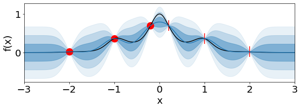
Figure 1: Invariant GP. Details in text.

An illustration of a simple invariance in 1D is shown in Figure 1. The true integrand in black is axis-symmetric which can be represented by the transformation $T_{1}(\boldsymbol{x})=-\boldsymbol{x}$. The set $G_{f}$ thus contains the identity transform $T_{0}$ as well as $T_{1}$. In the figure, the three observed points are marked as red dots. The invariant locations implied by $T_{1}$ are marked as red vertical bars. Even though these points are not observed, the model’s uncertainty shrinks at and around the implied locations. We want to highlight that using a standard GP with additional ‘fake’ observations at the invariant locations would cubicly increase the algorithmic cost of the method according to $\mathcal{O}(J^{3}N^{3})$. The invariant GP has complexity $\mathcal{O}(N^{3})$. Furthermore, samples from the invariant GP obey the invariant property as well, but samples from a standard GP with ‘fake’ observations do not. In the next section, we consider a subset of orthogonal transformations which allow for analytic computation of the required kernel integrals.

3.1 Orthogonal transformations

Consider that $G_{f}$ contains orthogonal transformations only, that is $T_{i}(\boldsymbol{x})=Q_{i}\boldsymbol{x}$, $i=1,\dots J$ with $Q_{i}$ a square matrix, and $Q_{i}^{\intercal}Q_{i}=\boldsymbol{I}$. Orthogonal transforms, among others, include rotations, point- and axis-projections. For the RBF-kernel introduced in Section 1, we can write the kernel mean for the $i$th and $j$th transform as:

$$qK_{ij}(\boldsymbol{x})=qK(Q_{i}^{\intercal}Q_{j}\boldsymbol{x})$$ (2)

where $qK$ is the kernel mean of the RBF-kernel without the transforms, evaluated at $\boldsymbol{s}_{ij}=Q_{i}^{\intercal}Q_{j}\boldsymbol{x}$. The equality is easily shown by re-arranging terms and using the orthogonal property of the $Q_{i}$. Eq. 2 might in itself be valuable as it allows for the computation of the mean estimator of the integral value $\mu_{Z}^{X}$. Unfortunately though, it is less straightforward to compute the double integrals $qKq_{ij}$ required for the integral variance $\sigma^{2,X}_{Z}$, and this may only be analytically possible for a subset of orthogonal transforms. One of those subsets are axis- and point symmetries, discussed in the next section.

3.2 Axis-flips and point-symmetries

For orthogonal transformations described in Section 3.1, and with a change of variables $Q_{i}^{\intercal}\circ Q_{j}:\Omega\rightarrow\mathbb{X}$, $Q_{i}^{\intercal}Q_{j}\boldsymbol{x}\mapsto\boldsymbol{s}_{ij}$, the variances $qKq_{ij}$ can be written as

$$qKq_{ij}=|\operatorname{det}^{-1}(Q_{i}^{\intercal}Q_{j})|\int_{Q_{i}^{\intercal}\circ Q_{j}(\Omega)}qK(\boldsymbol{s}_{ij})\pi(\boldsymbol{s}_{ij})\mathrm{d}\boldsymbol{s}_{ij}.$$ (3)

Even if the original integral $\int_{\Omega}qK(\boldsymbol{x})\pi(\boldsymbol{x})\mathrm{d}\boldsymbol{x}$ is analytic as is the case for the RBF-kernel, the linear transform $Q_{i}^{\intercal}Q_{j}$ generally distorts the integration domain as well as $\pi(\boldsymbol{x})$, yielding a possibly intractable integral. One way to circumvent this is to impose that the transform $Q_{i}^{\intercal}Q_{j}$ needs to be diagonal for all $i,j=1,...J$. There might be other scenarios where the integral remains analytic, here we only study this obvious case. This characteristic is fulfilled by $Q_{i}$ that encode axis- and point-symmetries, i.e, when the function $f$ is invariant under flipping the sign of one or more axis. Hence, the transformations are of the form $T_{i}(\boldsymbol{x})=Q_{i}\boldsymbol{x}$ with $Q_{i}^{kl}=c_{i}^{k}\delta_{kl}$ and $c_{i}^{k}\in\{-1,1\}$. One or multiple of sign-flips can be present separately in the set $G_{f}$. An illustration of several sets $\mathcal{A}(\boldsymbol{x})$ for different $G_{f}$, as well as the derivation of the necessary integrals are provided in Appendix B.

We will call a method encoding invariaces ‘invariant-BQ’ in contrast to ‘standard-BQ’. We highlight that the integration problem itself needs not be invariant (only $f$ does), as $\pi(\boldsymbol{x})$ or $\Omega$ need not be invariant. Further, the implied invariant observations influence the posterior consistently across symmetric planes or points as can be seen from Figure 1.

4 Experiments

We provide initial experiments that indicate increased sample efficiency of invariant-BQ in comparison to standard-BQ, on a set of synthetic examples, and a Fourier optics problem.

4.1 Synthetic examples

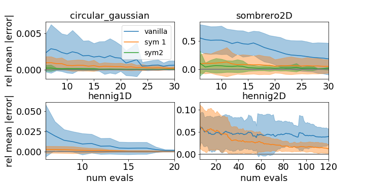
Figure 2: Average performance of standard-BQ and invariant-BQ on 4 synthetic examples.

We consider a collection of four simple functions implemented as quadrature test function in the Emukit Python library [18], all of which exhibit point- and/or axis symmetries (Appendix B.1 for definitions and illustrations). We apply invariant-BQ and integrate with respect to the Lebesgue measure $\pi(x)\equiv 1$ on a finite domain $\Omega=[-3,3]^{d}$ for each function, and compare the performance to standard-BQ.

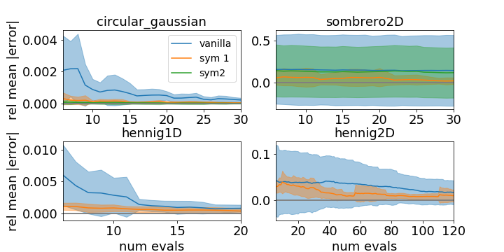
Figure 9: Same as Figure 2, but for Gaussian measure $\pi(\boldsymbol{x})$.

Figure 2 shows the relative mean absolute error between the mean estimator $\mu_{Z}$ and the true value of the integral, across 10 runs with different random seeds (Appendix D for experimental details). Not only does invariant-BQ (orange for point-, green for additional axis-symmetry) outperform the standard model (blue) on average at each step, it is also more stable as the estimate varies less between runs. Performance for a single run showing $\mu_{Z}$ and $\sigma_{Z}$ is plotted in Figure 8 in Appendix D. Figures 6 and 7 show the same experiment with optimal kernel hyperparameters $\lambda$ and $\theta$; the performance gain is even more apparent there. As a second experiment, we intgerate the same functions w.r.t. an isotropic Gaussian measure with density $\pi(\boldsymbol{x})=\mathcal{N}(\boldsymbol{x};\boldsymbol{b},l^{2}\boldsymbol{I})$, mean $\boldsymbol{b}=\mathbf{1}$ and variance $l^{2}=1$. As $\pi(\boldsymbol{x})$ is not invariant, neither is the product $f(\boldsymbol{x})\pi(\boldsymbol{x})$. The results are similar to the ones dicussed, and shown in Figure 9 in Appendix D.

4.2 Point spread function

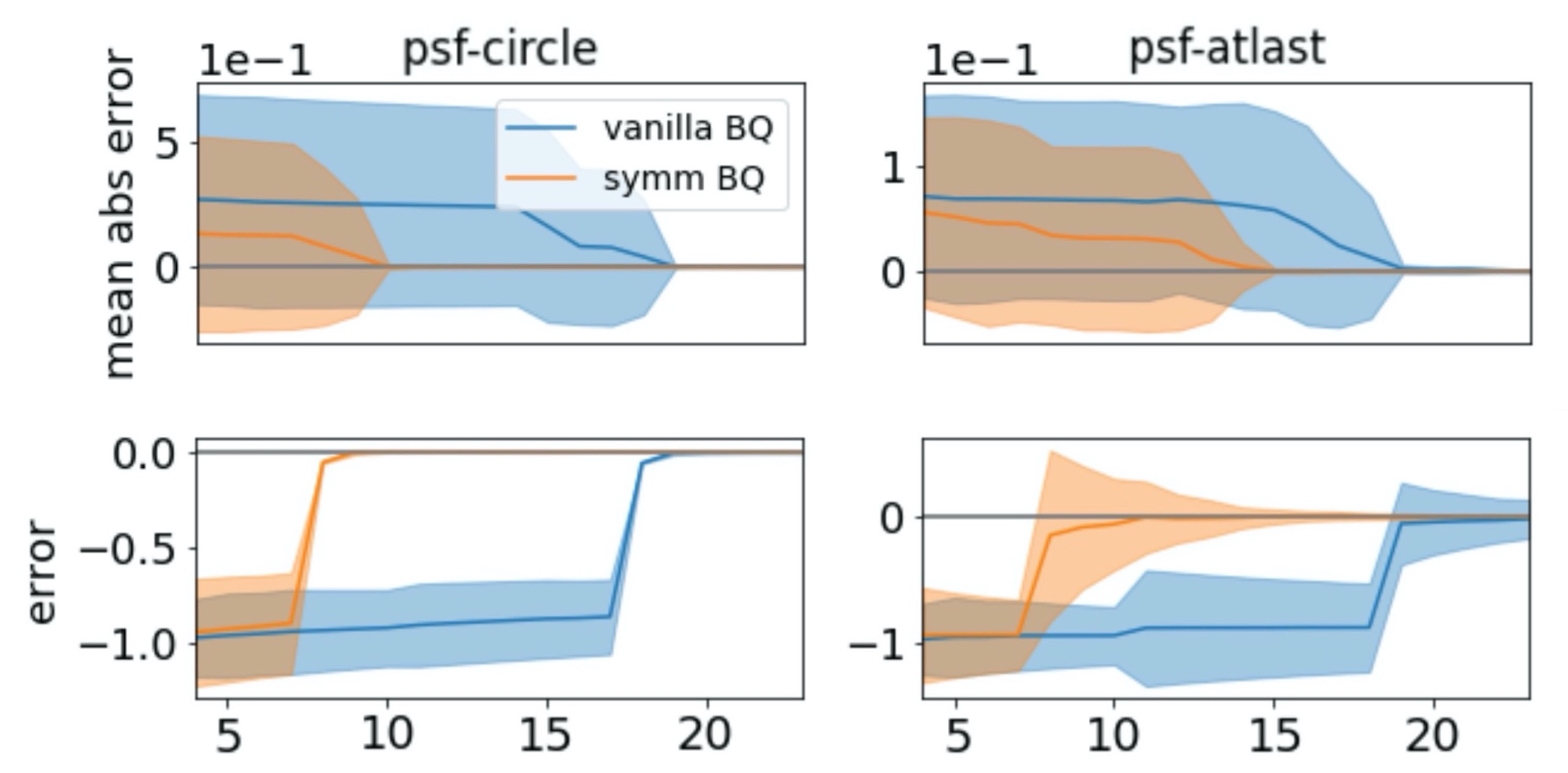
Figure 3: Average performance (t) vs a single run (b) on two PSFs; circular (l), ATLAST (r).

We apply invariant-BQ to approximate the integral of two point spread functions (PSFs). In Fourier optics, the point spread function is used to model the distribution of light in the image of a point formed by an optical system [1, 14]. See Appendix E for a description of the ATLAST and circular pupil used here. We use the poppy Python library [19] to generate pupil functions and their respective PSFs. The integral of the PSF is interpreted as the total power of the light source in the image, and used to normalise the PSF so it may be interpreted as a probability distribution. We compute the PSF for both the circular and the ATLAST pupil, both point-symmetric. The results are shown in Figure 3. Invariant-BQ consistently outperforms standard-BQ here.

5 Discussion & Conclusion

We proposed ‘invariant-BQ’, that leverages a GP prior encoding invariance of the integrand under a fixed set of input transformations. The integration measure and domain need not be invariant. We presented initial promising experiments that show improved sample efficiency over standard-BQ for a subset of transformations that allow for analytic GP inference. In future work it would be desirable to test invariant-BQ on a more complete set of experimental settings and baselines, and to study the effect on decision making and predictive model fidelity.

A: Formulas for Bayesian quadrature

Recall that we consider the problem of numerically approximating the integral $Z=\int_{\Omega}f(\boldsymbol{x})\pi(\boldsymbol{x})\>d\boldsymbol{x}$, $f:\mathbb{X}\rightarrow\mathbb{R}$, with integration domain $\Omega\subseteq\mathbb{X}\subseteq\mathbb{R}^{d}$ either a Cartesian product of finite bounds $[l_{1},u_{1}]\times...\times[l_{d},u_{d}]$, or the entire $\mathbb{R}^{d}$. The integration measure $\pi(\boldsymbol{x})$ is the Lebesgue measure $\pi(\boldsymbol{x})\equiv 1$, or the normal density $\mathcal{N}(\boldsymbol{x};\boldsymbol{\mu},\boldsymbol{\Sigma})$ respectively.

Recall that the integrand $f$ is modelled with a Gaussian process $f(\boldsymbol{x})\sim\mathcal{GP}(m(\boldsymbol{x}),k(\boldsymbol{x},\boldsymbol{x}^{\prime}))$ with mean function $m$ and kernel function $k$ that can be conditioned on integrand evaluations or ’data’ $D=\{(\boldsymbol{x}_{i},y_{i})\ |\ i=1..N\}$. The stacked observations are denoted as $Y\in\mathbb{R}^{N}$, and the corresponding stacked locations as $X\in\mathbb{R}^{N\times d}$. Then, the integral $Z\sim\mathcal{N}(\mu_{Z},\sigma^{2}_{Z})$ is 1D-normally distributed with scalar mean $\mu_{Z}$ and variance $\sigma^{2}_{Z}$:

$$\begin{split}\mu_{Z}&=\int_{\Omega}m(\boldsymbol{x})\pi(\boldsymbol{x})\>d\boldsymbol{x}+qK^{X}G^{-1}\Delta\\ \sigma^{2}_{Z}&=qKq-qK^{X}G^{-1}\left[qK^{X}\right]^{\intercal},\end{split}$$ (4)

where $G\in\mathbb{R}^{N\times N}$ is the kernel Gram matrix $G_{nm}=k(\boldsymbol{x}_{n},\boldsymbol{x}_{m})$, and $\Delta=Y-m(X)\in\mathbb{R}^{N}$ is the residual. Eq. 4 requires the computation of the kernel mean $qK^{X}:=\int_{\Omega}k(\boldsymbol{x},X)\pi(\boldsymbol{x})\mathrm{d}\boldsymbol{x}\in\mathbb{R}^{1\times N}$ evaluated at $X$, the scalar prior variance $qKq:=\iint_{\Omega\times\Omega}k(\boldsymbol{x},\boldsymbol{x}^{\prime})\pi(\boldsymbol{x})\pi(\boldsymbol{x}^{\prime})\mathrm{d}\boldsymbol{x}\mathrm{d}\boldsymbol{x}^{\prime}$, as well as the integral over the prior mean $\int_{\Omega}m(\boldsymbol{x})\pi(\boldsymbol{x})\mathrm{d}\boldsymbol{x}$. The kernel integrals cannot always be computed analytically. They can for certain kernels, such as the well-known squared exponential/ RBF-kernel $k(\boldsymbol{x},\boldsymbol{x}^{\prime})=\theta^{2}\exp(-\nicefrac{{\|\boldsymbol{x}-\boldsymbol{x}^{\prime}\|^{2}}}{{(2\lambda^{2})}})$, which is parametrized by its scalar variance $\theta^{2}$ and lengthscale $\lambda$. The integral over the prior mean function can be solved e.g., for a constant mean $m(\boldsymbol{x})=M$. These are the prior kernel we are considering in the paper.

B: Illustration of invariances in 2D

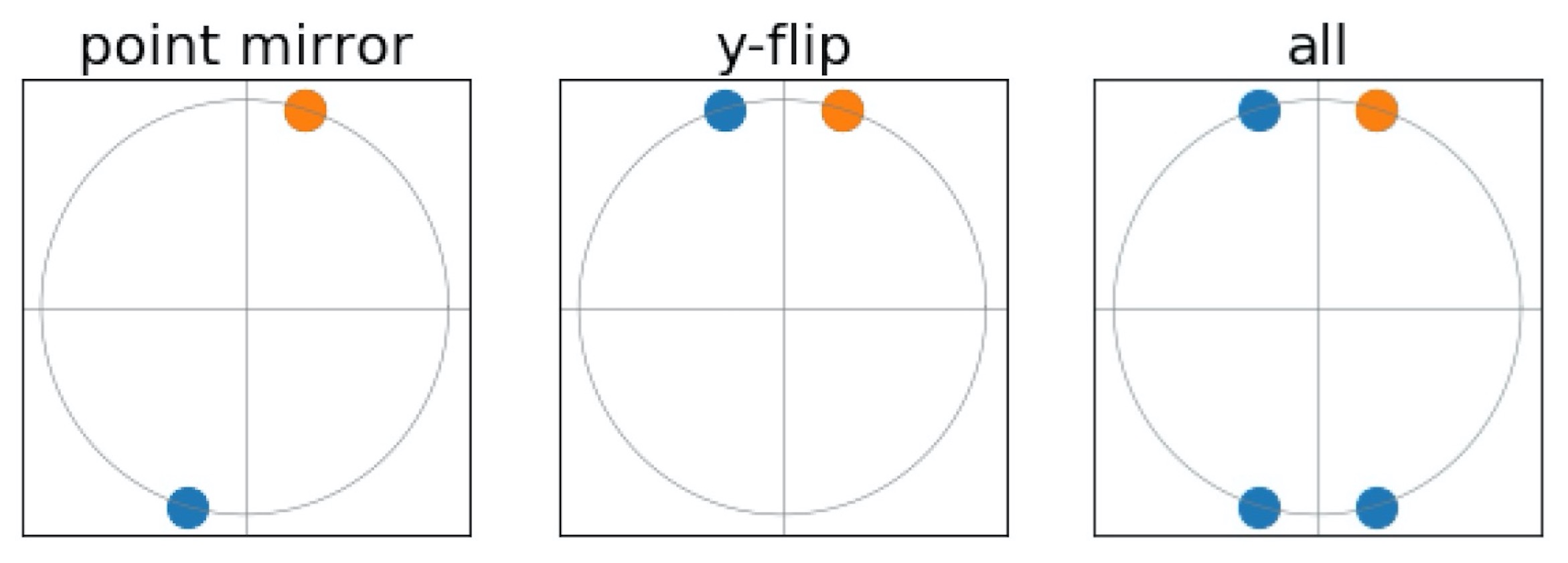
Figure 4: Set $\mathcal{A}(\boldsymbol{x})$ for point symmetry w.r.t. origin (left), y-axis flip (middle), and their combination (right). The point $\boldsymbol{x}=[0.3,1]^{\intercal}$ (orange) is same for all sets; the induced points are shown in blue. The size of set $G_{f}$ is $J=2,2$, and $4$ respectively.

Consider axis- and point-symmetries as in Section 3.2. The integration domain is transformed according to $Q_{i}^{\intercal}\circ Q_{j}(\Omega)$, which equals to flipping the integration bounds of dimension $q$ according to $(Q_{i}^{\intercal}Q_{j})_{qq}=c_{i}^{q}c_{j}^{q}\in\{-1,1\}$; the flip happens when the value is $-1$. The determinant of $Q_{i}^{\intercal}Q_{j}$ is either 1 or $-1$, and thus its absolute value is $1$. Figure 1 illustrates the 1D case, where $G_{f}$ consist only of $Q_{0}(x)=x$ and $Q_{1}(x)=-x$, thus $Q_{0}Q_{1}=Q_{1}Q_{0}=-1$, and $Q_{0}Q_{0}=Q_{1}Q_{1}=1$. In fact, for the special case of axis flips considered in this section, it is true that $Q_{i}^{\intercal}Q_{j}=Q_{j}^{\intercal}Q_{j}$ for all $i,j$. We provide an illustation of several sets $\mathcal{A}(\boldsymbol{x})$ for different $G_{f}$ for dimension $d=2$ in Figure 4.

C: Formulas for invariant BQ

Consider an invariant GP as introduced in Section 2. The distribution over the integral value $Z\sim\mathcal{N}(\mu_{Z},\sigma^{2}_{Z})$ remains Gaussian for invariant BQ. The posterior formulas for the mean and variance of the integral value are

$$\begin{split}\mu_{Z}&=\sum_{i=1}^{J}\int_{\Omega}m_{g}^{X}(T_{i}(\boldsymbol{x}))\pi(\boldsymbol{x})\mathrm{d}\boldsymbol{x}\\ \sigma^{2}_{Z}&=\sum_{i,j=1}^{J}\iint_{\Omega\times\Omega}k_{g}^{X}(T_{i}(\boldsymbol{x}),T_{j}(\boldsymbol{x}^{\prime}))\pi(\boldsymbol{x})\pi(\boldsymbol{x}^{\prime})\mathrm{d}\boldsymbol{x}\mathrm{d}\boldsymbol{x}^{\prime},\end{split}$$ (5)

where the superscript ^X indicates that the Gaussian process $g$ is conditioned on the $N$ integrand observations $Y$ at locations $X$. We expand the expressions above:

$$\begin{split}\mu_{Z}&=\sum_{i=1}^{J}\int_{\Omega}m_{g}(T_{i}(\boldsymbol{x}))\pi(\boldsymbol{x})\mathrm{d}\boldsymbol{x}+\sum_{i,j=1}^{J}qK^{X}_{ij}G^{-1}\Delta\\ \sigma^{2}_{Z}&=\sum_{i,j=1}^{J}qKq_{ij}-\sum_{i,j=1}^{J}qK^{X}_{ij}G^{-1}\sum_{k,l=1}^{J}qK^{X\intercal}_{kl},\end{split}$$ (6)

with $G_{nm}=\sum_{i,j=1}^{J}k(T_{i}(\boldsymbol{x}_{n}),T_{j}(\boldsymbol{x}_{m}))$ the kernel Gram matrix, and $qK_{ij}^{X}:=\int_{\Omega}k(T_{i}(\boldsymbol{x}),T_{j}(X))\pi(\boldsymbol{x})\mathrm{d}\boldsymbol{x}$, the kernel mean corresponding to invariances $T_{i}$ and $T_{j}$ evaluated at $X$, and $qKq_{ij}:=\iint_{\Omega\times\Omega}k_{g}(T_{i}(\boldsymbol{x}),T_{j}(\boldsymbol{x}^{\prime}))\pi(\boldsymbol{x})\pi(\boldsymbol{x}^{\prime})\mathrm{d}\boldsymbol{x}\mathrm{d}\boldsymbol{x}^{\prime}$ the prior variance corresponding to invariances $T_{i}$ and $T_{j}$. Note that $qK_{ij}^{X}$ is a row vector of size $N$, where $N$ is the number of observations, $qKq_{ij}$ is a scalar. Even if the (double) integrals of $qK(\boldsymbol{x})$ and $k(\boldsymbol{x},\boldsymbol{x}^{\prime})$ are known analytically, the integrals $qK_{i}^{X}$ and $qKq_{ij}$ might be arbitrarily complicated or even intractable.

C: The synthetic functions considered for invariant-BQ

All functions are taken from the BQ test function folder of the Emukit library [18]. They are:

$$\begin{split}&\mathop{\text{hennig1D}}(x)=e^{-x^{2}-\sin^{2}(3x)}\\ &\mathop{\text{hennig2D}}(\boldsymbol{x})=e^{-\sin(3\|\boldsymbol{x}\|^{2})-\boldsymbol{x}^{T}S\boldsymbol{x}},\quad S=\begin{bmatrix}1&0.5\\ 0.5&1\end{bmatrix}\\ &\mathop{\text{circular\_gaussian}}(\boldsymbol{x})=\frac{1}{2\pi\sigma^{2}}\|\boldsymbol{x}\|^{2}e^{-\frac{\left(\|\boldsymbol{x}\|-\mu\right)^{2}}{2\sigma^{2}}}\\ &\hskip 142.26378pt\ \mu\in\mathbb{R},\sigma>0\\ &\mathop{\text{sombrero2D}}(\boldsymbol{x})=\frac{\sin(\pi\|\boldsymbol{x}\|c)}{\pi\|\boldsymbol{x}\|c},\quad c\in\mathbb{R}_{+}.\end{split}$$

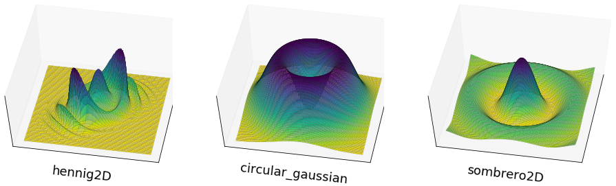
Figure 5: Three out of the four test functions, used in Figures 2 and 8. Plot boundaries coincide with integration domain. All are point-symmetric w.r.t. the origin, 2 and 3 are also axis-symmetric.

D: Additional results of synthetic experiments in Section 4.1

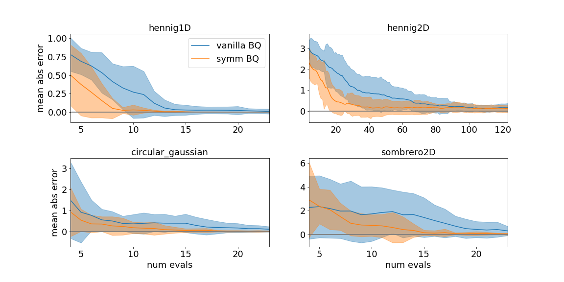
Figure 6: Plots as in Figure 2 but for optimal hyper-parameters $\lambda$ and $\theta$.

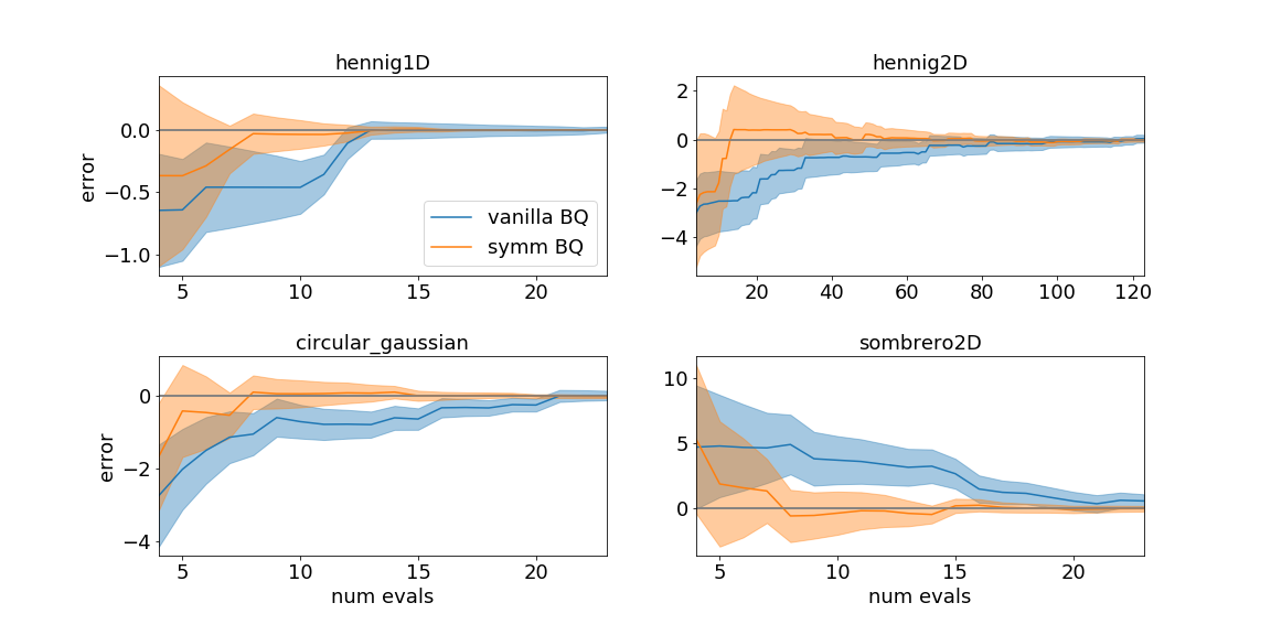
Figure 7: Plots as in Figure 8 but for optimal hyper-parameters $\lambda$ and $\theta$.

Experimental details of synthetic experiments: Observation locations are selected sequentially and actively by maximizing the integral variance reduction acquisition function [7]. Figure 2 in the main paper shows the relative mean absolute error between the mean estimator $\mu_{Z}$ and the true value of the integral, across 10 runs with different random seeds. The runs differ in the initial design which consist of 5 randomly chosen location in $\Omega$ and are shared by all algorithms. Invariant-BQ uses point symmetry (orange) as well as all symmetries (green) as in Figure 4, most left and most right plot, respectively.

Figures 6 and 7 contain additional results for the synthetic examples as described in Section 4.1. In contrast to Figures 2 and 8 where the kernel hyperparameters $\lambda$ and $\theta$ where set by maximizing the marginal log-likelihood of the model, here the hyperparameters are set to optimal values (found by over-sampling). This means that in cases where hyper-paramters are known, the performance improvements of invariant-BQ over standard-BQ are even more apparent.

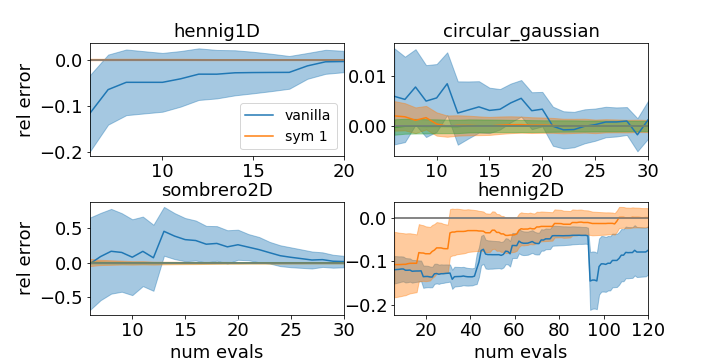
Figure 8: Performance for a single run taken from the runs of Figure 2. Details in text.

In addition to visualising performance on synthetic examples averaged over multiple runs in Figure 2, we plot a single run below. Here, the solid lines show the error between $\mu_{Z}$ and the true integral value, and the shaded areas show the standard deviation $\sigma_{Z}$ of the posterior.

E: Additional results of point spread function in Section 4.2

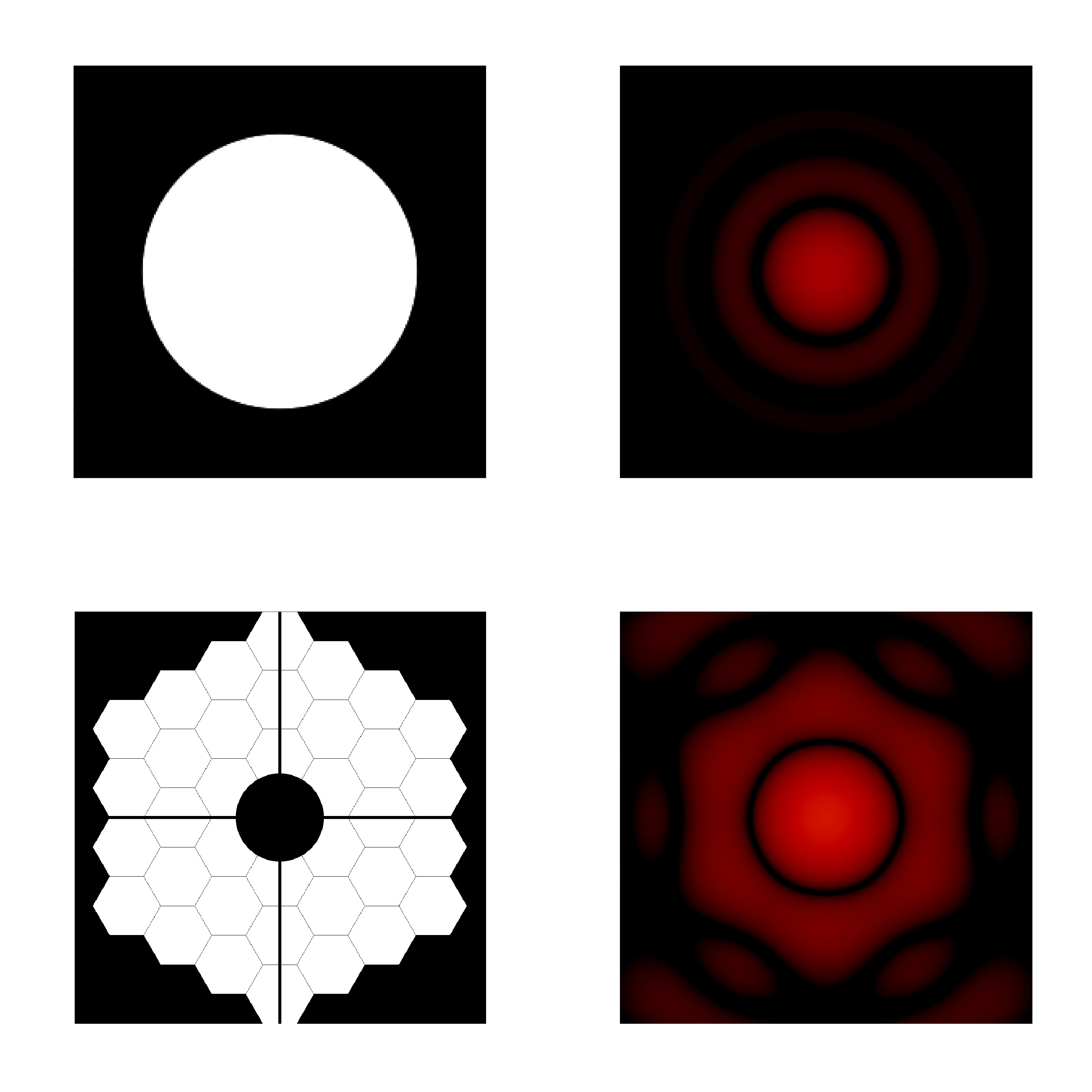
Figure 10: Pupil function (left) and PSF (right) for a perfect circular lens (top) and ATLAST (bottom). The PSF is computed for the wavelength $2\times 10^{-5}$

The point spread function (PSF) is defined as the absolute square of the Fourier transform of the pupil function, which is a complex function used to define the physical size and shape of the lens.

The PSF for a perfect circular lens focused onto the point source is known as the Airy pattern. For a complex segmented pupil, the PSF becomes more peculiar in its geometry, increasingly so depending on the number of composing segments and obscurations. This can be seen in Figure 10, where we plot the pupil function and PSF for the ATLAST pupil [20, 6], a pupil composed of three rings of two-metre segments with an added central obscuration and a spider pattern.

References

- [1] Pablo Artal “Handbook of Visual Optics, Volume Two: Instrumentation and Vision Correction” CRC Press, 2017
- [2] F.-X. Briol, C.. Oates, M. Girolami, M.. Osborne and D. Sejdinovic “Probabilistic Integration: A Role in Statistical Computation?” In Statistical Science 34.1 The Institute of Mathematical Statistics, 2019, pp. 1–22 DOI: 10.1214/18-STS660
- [3] Henry R. Chai and Roman Garnett “Improving Quadrature for Constrained Integrands” In The 22nd International Conference on Artificial Intelligence and Statistics, AISTATS 2019, 16-18 April 2019, Naha, Okinawa, Japan, 2019, pp. 2751–2759 URL: http://proceedings.mlr.press/v89/chai19a.html
- [4] J. Cockayne, C. Oates, T. Sullivan and M. Girolami “Bayesian Probabilistic Numerical Methods” In arXiv:1702.03673 [stat.ME], 2017
- [5] P. Diaconis “Bayesian numerical analysis” In Statistical Decision Theory and Related Topics IV 1 Springer-Verlag, New York, 1988, pp. 163–175
- [6] Lee D Feinberg, Andrew Jones, Gary Mosier, Norman Rioux, Dave Redding and Mike Kienlen “A cost-effective and serviceable ATLAST 9.2 m telescope architecture” In Space Telescopes and Instrumentation 2014: Optical, Infrared, and Millimeter Wave 9143, 2014, pp. 914316 International Society for OpticsPhotonics
- [7] Alexandra Gessner, Javier Gonzalez and Maren Mahsereci “Active Multi-Information Source Bayesian Quadrature” In CoRR abs/1903.11331, 2019 arXiv: http://arxiv.org/abs/1903.11331
- [8] T. Gunter, M.. Osborne, R. Garnett, P. Hennig and S.. Roberts “Sampling for Inference in Probabilistic Models with Fast Bayesian Quadrature” In Advances in Neural Information Processing Systems 27, 2014, pp. 2789–2797 URL: http://arxiv.org/abs/1411.0439
- [9] P. Hennig, M.. Osborne and M. Girolami “Probabilistic numerics and uncertainty in computations” In Proceedings of the Royal Society of London A: Mathematical, Physical and Engineering Sciences 471.2179, 2015
- [10] M. Kanagawa and P. Hennig “Convergence Guarantees for Adaptive Bayesian Quadrature Methods” In Advances in Neural Information Processing Systems 32 Curran Associates, Inc., 2019, pp. 6234–6245 URL: https://papers.nips.cc/paper/8854-convergence-guarantees-for-adaptive-bayesian-quadrature-methods
- [11] Toni Karvonen and Simo Särkkä “Fully symmetric kernel quadrature” arXiv: 1703.06359 In arXiv:1703.06359 [cs, math, stat], 2017 URL: http://arxiv.org/abs/1703.06359
- [12] F.. Larkin “Gaussian measure in Hilbert space and applications in numerical analysis” In Rocky Mountain J. Math. 2.3 Rocky Mountain Mathematics Consortium, 1972, pp. 379–422 DOI: 10.1216/RMJ-1972-2-3-379
- [13] Yifei Ma, Roman Garnett and Jeff Schneider “Active Area Search via Bayesian Quadrature” In Proceedings of the Seventeenth International Conference on Artificial Intelligence and Statistics 33, Proceedings of Machine Learning Research Reykjavik, Iceland: PMLR, 2014, pp. 595–603 URL: http://proceedings.mlr.press/v33/ma14.html
- [14] V.N. Mahajan “Optical Imaging and Aberrations: Ray geometrical optics”, Optical Imaging and Aberrations pts. 1-2 SPIE Optical Engineering Press, 1998 URL: https://books.google.co.uk/books?id=Jg1JW4kWD1UC
- [15] A. O’Hagan “Bayes-Hermite Quadrature” In Journal of Statistical Planning and Inference 29, 1991, pp. 245–260
- [16] M. Osborne, R. Garnett, Z. Ghahramani, D.. Duvenaud, S.. Roberts and C.. Rasmussen “Active Learning of Model Evidence Using Bayesian Quadrature” In Advances in Neural Information Processing Systems 25, 2012, pp. 46–54 URL: http://papers.nips.cc/paper/4657-active-learning-of-model-evidence-using-bayesian-quadrature.pdf
- [17] M. Osborne, R. Garnett, S. Roberts, C. Hart, S. Aigrain and N Gibson “Bayesian Quadrature for Ratios” In Proceedings of the Fifteenth International Conference on Artificial Intelligence and Statistics 22, Proceedings of Machine Learning Research PMLR, 2012, pp. 832–840 URL: http://proceedings.mlr.press/v22/osborne12.html
- [18] Andrei Paleyes, Mark Pullin, Maren Mahsereci, Neil Lawrence and Javier González “Emulation of physical processes with Emukit” In Second Workshop on Machine Learning and the Physical Sciences, NeurIPS, 2019
- [19] Marshall Perrin, Joseph Long, Ewan Douglas, Neil Zimmerman, Anand Sivaramakrishnan, Shannon Osborne, Kyle Douglass, Maciek Grochowicz, Phillip Springer and Ted Corcovilos “The Poppy Library” In GitHub repository GitHub, https://github.com/spacetelescope/poppy, 2011
- [20] Marc Postman, Thomas M Brown, Kenneth R Sembach, Jason Tumlinson, C Matt Mountain, Rémi Soummer, Mauro Giavalisco, Daniela Calzetti, Wesley Traub and Karl R Stapelfeldt “Advanced technology large-aperture space telescope: science drivers and technology developments” In Optical Engineering 51.1 International Society for OpticsPhotonics, 2012, pp. 011007
- [21] C.. Rasmussen and Z. Ghahramani “Bayesian Monte Carlo” In Advances in Neural Information Processing Systems 15 Cambridge, MA, USA: MIT Press, 2003, pp. 489–496 Max-Planck-Gesellschaft
- [22] C.. Rasmussen and C… Williams “Gaussian Processes for Machine Learning”, Adaptive Computation and Machine Learning Cambridge, MA, USA: MIT Press, 2006, pp. 248 Max-Planck-Gesellschaft
- [23] Mark Wilk, Matthias Bauer, ST John and James Hensman “Learning Invariances using the Marginal Likelihood” In Advances in Neural Information Processing Systems 31 Curran Associates, Inc., 2018, pp. 9938–9948 URL: http://papers.nips.cc/paper/8199-learning-invariances-using-the-marginal-likelihood.pdf
- [24] X. Xi, F.-X. Briol and M. Girolami “Bayesian Quadrature for Multiple Related Integrals” In Proceedings of the 35th International Conference on Machine Learning 80, Proceedings of Machine Learning Research PMLR, 2018, pp. 5373–5382 URL: http://proceedings.mlr.press/v80/xi18a.html
—Supplementary Material—