Simulations: Scheduling to learn

1 Experiments

In this section we provide the empirical studies comparing the performances, in terms of total utility, of the Algorithm 1 and Algorithm 2 mentioned in section 3 above. In all the respective experiments followed we cap the respective total running time to some $T$ and evaluate the performance of Algorithm 1 and Algorithm 2, where Algorithm 1 runs for the entire time horizon $T$ since it’s given the confusion matrices and Algorithm 2 first learns the confusion matrices for some time and then follows the Greedy algorithm. The evaluations are made on one synthetic dataset and two real datasets.

1.1 Synthetic Data

For synthetic data we generate $m$= 30 workers, and $n$ binary tasks, where $n\in\{5,15,25,45,\cdots 1250\}$. Here $n$ can be interpreted as time slots reserved to learn the confusion matrices for Algorithm 2. The true label of each task is uniformly sampled from $\{1,2\}$. The number of incoming samples follow a poisson distribution with $\lambda=5$ and the $w_{s}$ for each incoming sample is sampled randomly from [3,4,5,6,7,8,9,10].

For each worker, the 2-by-2 confusion matrix is generated as follows: the diagonal entries of confusion matrix for each worker $C_{i}(j,j)$ is given by $p_{i}=0.9-0.005\times i$, where index, $i$ goes from 0 to 30. The obtained 30 confusion matrices are then shuffled randomly and assigned to 30 workers.

After the data is generated the experiment is performed as follows, a. we fix the total time horizon $T$ as 10,000, b.1 Incoming data is sent to Algorithm 1 and Algorithm 2, b.2 Algorithm 1 keeps generating utility throughout the time horizon, while Algorithm 2 trades initial utility by using initial incoming samples to learn its confusion matrices till $n_{i}$ time units, c.1 now for first set of data we have $n_{1}=5$ or we send samples across 5 time units to all the workers for labelling, c.2 the labels obtained are passed through the Opt-D&S algorithm mentioned in [4] to learn the confusion matrices for Algorithm 2, d. from time $n_{1}$ onward both Algorithm 1 and Algorithm 2 generate utility, e. we keep on doing this process for all binary tasks with $n\in\{5,15,25,35,45,50,150,250,350,450,500,750,1000,1250\}$.

We perform 5 iterations, for each binary task with reserved $n_{i}$ time slots, of the above mentioned process to get better estimate of the utility from both Algorithm 1 and Algorithm 2. The main evaluation is with regards to the total utility generated, across all the incoming samples, by passing the samples via Algorithm 1 and Algorithm 2. Even before running the simulations common logic would suggest that for algorithm 2 there’s a trade-off between time spent learning and gain in utility. Which is exactly what we see in out simulation results.

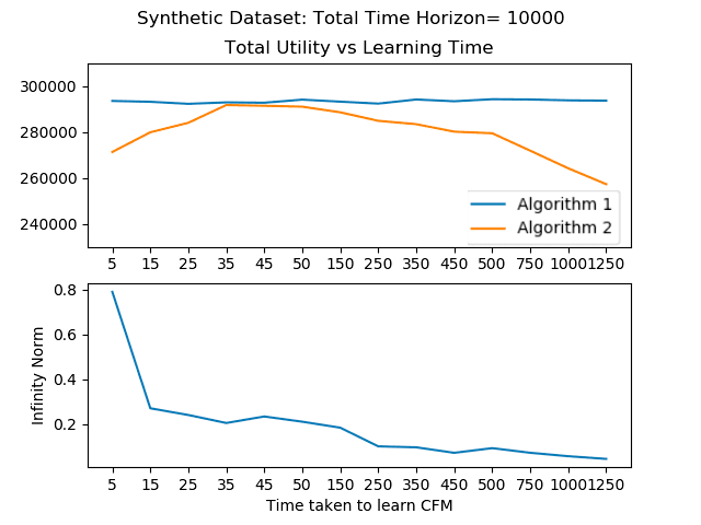
Figure 1: Total Utility and Infinity norm as a function of learning time for synthetic data

1.2 Real Data

For real data experiments, we compare the algorithms on two datasets: the binary Bird dataset [5] which has labels of bird species, and the multi-class DOG dataset [6] which has labels for the breed of a dog. The Bird dataset [5] has $m=39$ workers, and 108 samples in total. While from the DOG dataset [6] we use $m=90$ workers and it has 798 samples in total. Like mentioned for the synthetic dataset, the number of incoming samples follow a poisson distribution with $\lambda=5$ and the $w_{s}$ for each incoming sample is sampled randomly from [3,4,5,6,7,8,9,10].

We modified the multi-class DOG dataset [6] as binary dataset by clubbing classes together, more specifically we assigned (1,2) as class 1 and (3,4) as class 2.

We then performed the same procedure mentioned in the above subsection, the only difference being that we run it for both the algorithms on both the datasets for a total time horizon of 4000 units, and the original confusion matrix is replaced by the confusion matrix generated by Opt-D&S algorithm from [4] using maximum samples available for each respective datasets.

Our experimental results on real datasets are consistent with the results from synthetic datasets. There is indeed a trade-off between time spent learning and total utility. One peculiar thing to observe from the results of DOG dataset [6] however is that in its case the confusion matrices are very well learnt since the beginning due to high number of samples, 252, which are required due to sparsity of the dataset and due to the fact that we require each worker to label at least one sample.

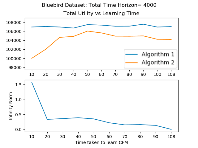
(a) BIRD data

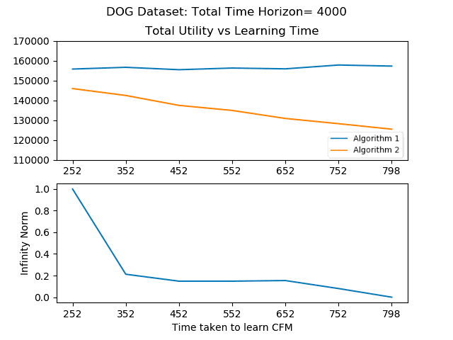
(b) DOG data

Figure 2: Total Utility and Infinity norm as a function of learning time on real datasets

References

- [1] Not Just Age but Age and Quality of Information by Nived Rajaraman, Rahul Vaze, Goonwanth Reddy. https://arxiv.org/abs/1812.08617
- [2] Pareto Optimal Streaming Unsupervised Classification by Soumya Basu, Steven Gutstein, Brent Lance, Sanjay Shakkottai. http://proceedings.mlr.press/v97/basu19a/basu19a.pdf
- [3] An Online Learning Approach to Improving the Quality of Crowd-Sourcing by Yang Liu, Mingyan Liu. https://ieeexplore.ieee.org/document/7892023
- [4] Spectral Methods meet EM: A Provably Optimal Algorithm for Crowdsourcing by Yuchen Zhang, Xi Chen, Dengyong Zhou, Michael I. Jordan https://arxiv.org/pdf/1406.3824.pdf
- [5] P. Welinder, S. Branson, S. Belongie, and P. Perona. The multidimensional wisdom of crowds. In Advances in Neural Information Processing Systems, volume 10, pages 2424–2432, 2010.
- [6] J. Deng, W. Dong, R. Socher, L.-J. Li, K. Li, and L. Fei-Fei. Imagenet: A large-scale hier- archical image database. In IEEE Conference on Computer Vision and Pattern Recognition, 2009.