Multiscale Vision Transformers for Image Classification and Object Detection

MViTv2: Improved Multiscale Vision Transformers
for Classification and Detection

Abstract

In this paper, we study Multiscale Vision Transformers (MViTv2) as a unified architecture for image and video classification, as well as object detection. We present an improved version of MViT that incorporates decomposed relative positional embeddings and residual pooling connections. We instantiate this architecture in five sizes and evaluate it for ImageNet classification, COCO detection and Kinetics video recognition where it outperforms prior work. We further compare MViTv2s’ pooling attention to window attention mechanisms where it outperforms the latter in accuracy/compute. Without bells-and-whistles, MViTv2 has state-of-the-art performance in 3 domains: 88.8% accuracy on ImageNet classification, 58.7 AP${}^{\text{box}}$ on COCO object detection as well as 86.1% on Kinetics-400 video classification. Code and models are available at https://github.com/facebookresearch/mvit.

1 Introduction

Designing architectures for different visual recognition tasks has been historically difficult and the most widely adopted ones have been the ones that combine simplicity and efficacy, e.g. VGGNet [67] and ResNet [37]. More recently Vision Transformers (ViT) [17] have shown promising performance and are rivaling convolutional neural networks (CNN) and a wide range of modifications have recently been proposed to apply them to different vision tasks [21, 1, 2, 55, 90, 68, 73, 78].

While ViT [17] is popular in image classification, its usage for high-resolution object detection and space-time video understanding tasks remains challenging. The density of visual signals poses severe challenges in compute and memory requirements as these scale quadratically in complexity within the self-attention blocks of Transformer-based [76] models. The community has approached this burden with different strategies: Two popular ones are (1) local attention computation within a window [55] for object detection and (2) pooling attention that locally aggregates features before computing self-attention in video tasks [21].

The latter fuels Multiscale Vision Transformers (MViT) [21], an architecture that extends ViT in a simple way: instead of having a fixed resolution throughout the network, it has a feature hierarchy with multiple stages starting from high-resolution to low-resolution. MViT is designed for video tasks where it has state-of-the-art performance.

(a)

(b)

(c)

Figure 1: Our MViTv2 is a multiscale transformer with state-of-the-art performance across three visual recognition tasks.

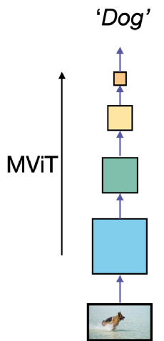
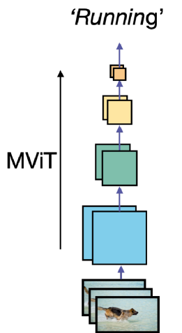
In this paper, we develop two simple technical improvements to further increase its performance and study MViT as a single model family for visual recognition across 3 tasks: image classification, object detection and video classification, in order to understand if it can serve as a general vision backbone for spatial as well as spatiotemporal recognition tasks (see Fig. 1). Our empirical study leads to an improved architecture (MViTv2) and encompasses the following:

(i) We create strong baselines that improve pooling attention along two axes: (a) shift-invariant positional embeddings using decomposed location distances to inject position information in Transformer blocks; (b) a residual pooling connection to compensate the effect of pooling strides in attention computation. Our simple-yet-effective upgrades lead to significantly better results.

(ii) Using the improved structure of MViT, we employ a standard dense prediction framework: Mask R-CNN [36] with Feature Pyramid Networks (FPN) [53] and apply it to object detection and instance segmentation.

We study if MViT can process high-resolution visual input by using pooling attention to overcome the computation and memory cost involved. Our experiments suggest that pooling attention is more effective than local window attention mechanisms (e.g. Swin [55]). We further develop a simple-yet-effective Hybrid window attention scheme that can complement pooling attention for better accuracy/compute tradeoff.

(iii) We instantiate our architecture in five sizes of increasing complexity (width, depth, resolution) and report a practical training recipe for large multiscale transformers. The MViT variants are applied to image classification, object detection and video classification, with minimal modification, to study its purpose as a generic vision architecture.

Experiments reveal that our MViTv2 achieves 88.8% accuracy for ImageNet-1K classification, with pretraining on ImageNet-21K (and 86.3% without), as well as 58.7 AP${}^{\text{box}}$ on COCO object detection using only Cascade Mask R-CNN [6]. For video classification tasks, MViT achieves unprecedented accuracies of 86.1% on Kinetics-400, 87.9% on Kinetics-600, 79.4% on Kinetics-700, and 73.3% on Something-Something-v2. Our video code will be open-sourced in PyTorchVideo ${}^{\text{,}}$ [20, 19].

2 Related Work

CNNs

serve as the primary backbones for computer vision tasks, including image recognition [48, 46, 67, 69, 39, 10, 71, 62, 34, 15], object detection [38, 29, 53, 6, 63, 93] and video recognition [66, 25, 8, 61, 51, 84, 75, 23, 79, 28, 22, 92, 42].

Vision transformers

have generated a lot of recent enthusiasm since the work of ViT [17], which applies a Transformer architecture on image patches and shows very competitive results on image classification. Since then, different works have been developed to further improve ViT, including efficient training recipes [73], multi-scale transformer structures [21, 55, 78] and advanced self-attention mechanism design [21, 55, 11]. In this work, we build upon the Multiscale Vision Transformers (MViT) and study it as a general backbone for different vision tasks.

Vision transformers for object detection

tasks [55, 89, 78, 11] address the challenge of detection typically requiring high-resolution inputs and feature maps for accurate object localization. This significantly increases computation complexity due to the quadratic complexity of self-attention operators in transformers [76]. Recent works develop technology to alleviate this cost, including shifted window attention [55] and Longformer attention [89]. Meanwhile, pooling attention in MViT is designed to compute self-attention efficiently using a different perspective [21]. In this work, we study MViT for detection and more generally compare pooling attention to local attention mechanisms.

Vision transformers for video recognition

have also recently shown strong results, but mostly [59, 3, 1, 56] rely on pre-training with large-scale external data (e.g. ImageNet-21K [14]). MViTv1 [21] reports a good training-from-scratch recipe for Transformer-based architectures on Kinetics data [44]. In this paper, we use this recipe and improve the MViT architecture with improved pooling attention which is simple yet effective on accuracy; further, we study the (large) effect of ImageNet pre-training for video tasks.

3 Revisiting Multiscale Vision Transformers

The key idea of MViTv1 [21] is to construct different stages for both low- and high-level visual modeling instead of single-scale blocks in ViT [17]. MViT slowly expands the channel width $D$, while reducing the resolution $L$ (i.e. sequence length), from input to output stages of the network.

To perform downsampling within a transformer block, MViT introduces Pooling Attention. Concretely, for an input sequence, $X\in\mathbb{R}^{L\times D}$, it applies linear projections ${{W}}_{Q}$, ${{W}}_{K}$, ${{W}}_{V}\in\mathbb{R}^{D\times D}$ followed by pooling operators ($\mathcal{P}$) to query, key and value tensors, respectively:

$$Q=\mathcal{P}_{Q}\left(XW_{Q}\right),\ K=\mathcal{P}_{K}\left(XW_{K}\right),\ V=\mathcal{P}_{V}\left(XW_{V}\right),$$ (1)

where the length $\tilde{L}$ of $Q\in\mathbb{R}^{\tilde{L}\times D}$ can be reduced by $\mathcal{P}_{Q}$ and $K$ and $V$ length can be reduced by $\mathcal{P}_{K}$ and $\mathcal{P}_{V}$.

Subsequently, pooled self-attention,

$$Z:=\mathrm{Attn}(Q,K,V)=\mathrm{Softmax}\left(QK^{\top}/\sqrt{D}\right)V,$$ (2)

computes the output sequence $Z\in\mathbb{R}^{\tilde{L}\times D}$ with flexible length $\tilde{L}$. Note that the downsampling factors $\mathcal{P}_{K}$ and $\mathcal{P}_{V}$ for key and value tensors can be different from the ones applied to the query sequence, $\mathcal{P}_{Q}$.

Pooling attention enables resolution reduction between different stages of MViT by pooling the query tensor $Q$, and to significantly reduce compute and memory complexity by pooling the key, ${K}$, and value, ${V}$, tensors.

4 Improved Multiscale Vision Transformers

In this section, we first introduce an empirically powerful upgrade to pooling attention (§4.1). Then we describe how to employ our generic MViT architecture for object detection (§4.2) and video recognition (§4.3). Finally, §4.4 shows five concrete instantiations for MViTv2 in increasing complexity.

4.1 Improved Pooling Attention

We start with re-examining two important implications of MViTv2 for potential improvement and introduce techniques to understand and address them.

Figure 2: The improved Pooling Attention mechanism that incorporating decomposed relative position embedding, ${{R}}_{p(i),p(j)}$, and residual pooling connection modules in the attention block.

Decomposed relative position embedding.

While MViT has shown promises in their power to model interactions between tokens, they focus on content, rather than structure. The space-time structure modeling relies solely on the “absolute” positional embedding to offer location information. This ignores the fundamental principle of shift-invariance in vision [47]. Namely, the way MViT models the interaction between two patches will change depending on their absolute position in images even if their relative positions stay unchanged. To address this issue, we incorporate relative positional embeddings [65], which only depend on the relative location distance between tokens into the pooled self-attention computation.

We encode the relative position between the two input elements, $i$ and $j$, into positional embedding ${{R}}_{p(i),p(j)}\in\mathbb{R}^{d}$, where $p(i)$ and $p(j)$ denote the spatial (or spatiotemporal) position of element $i$ and $j$. The pairwise encoding representation is then embedded into the self-attention module:

$$\mathrm{Attn}(Q,K,V)=\mathrm{Softmax}\left((QK^{\top}+E^{(\mathrm{rel})})/\sqrt{d}\right)V,$$

$$\text{where \quad}E^{(\mathrm{rel})}_{ij}=Q_{i}\cdot R_{p(i),p(j)}.$$ (3)

However, the number of possible embeddings $R_{p(i),p(j)}$ scale in $\mathcal{O}(TWH)$, which can be expensive to compute. To reduce complexity, we decompose the distance computation between element $i$ and $j$ along the spatiotemporal axes:

$${{R}}_{p(i),p(j)}={{R}}_{h(i),h(j)}^{\mathrm{h}}+{{R}}_{w(i),w(j)}^{\mathrm{w}}+{{R}}_{t(i),t(j)}^{\mathrm{t}},$$ (4)

where $R^{\mathrm{h}},R^{\mathrm{w}},R^{\mathrm{t}}$ are the positional embeddings along the height, width and temporal axes, and $h(i)$, $w(i)$, and $t(i)$ denote the vertical, horizontal, and temporal position of token $i$, respectively. Note that $R^{\mathrm{t}}$ is optional and only required to support temporal dimension in the video case. In comparison, our decomposed embeddings reduce the number of learned embeddings to $\mathcal{O}(T+W+H)$, which can have a large effect for early-stage, high-resolution feature maps.

Residual pooling connection.

As demonstrated [21], pooling attention is very effective to reduce the computation complexity and memory requirements in attention blocks. MViTv1 has larger strides on ${K}$ and ${V}$ tensors than the stride of the ${Q}$ tensors which is only downsampled if the resolution of the output sequence changes across stages. This motivates us to add the residual pooling connection with the (pooled) ${Q}$ tensor to increase information flow and facilitate the training of pooling attention blocks in MViT.

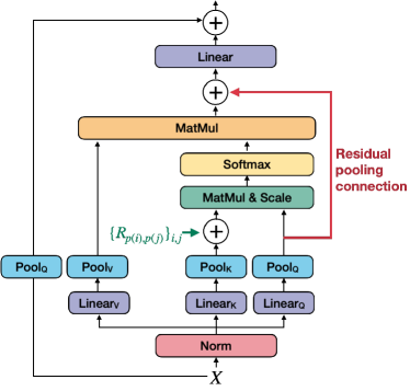
We introduce a new residual pooling connection inside the attention blocks as shown in Fig. 2. Specifically, we add the pooled query tensor to the output sequence ${Z}$. So Eq. (2) is reformulated as:

$$Z:=\mathrm{Attn}\left(Q,K,V\right)+Q.$$ (5)

Note that the output sequence ${Z}$ has the same length as the pooled query tensor $Q$.

The ablations in §6.2 and §5.3 shows that both the pooling operator ($\mathcal{P}_{Q}$) for query $Q$ and the residual path are necessary for the proposed residual pooling connection. This change still enjoys the low-complexity attention computation with large strides in key and value pooling as adding the pooled query sequence in Eq. (5) comes at a low cost.

4.2 MViT for Object Detection

In this section, we describe how to apply the MViT backbone for object detection and instance segmentation tasks.

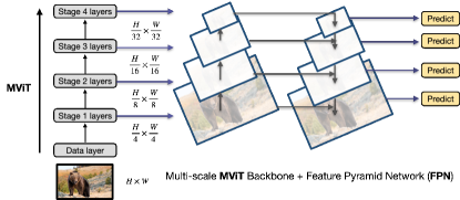
FPN integration.

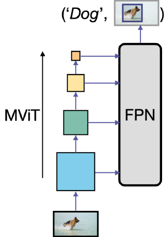
The hierarchical structure of MViT produces multiscale feature maps in four stages, and therefore naturally integrates into Feature Pyramid Networks (FPN) [53] for object detection tasks, as shown in Fig. 3. The top-down pyramid with lateral connections in FPN constructs semantically strong feature maps for MViT at all scales. By using FPN with the MViT backbone, we apply it to different detection architectures (e.g. Mask R-CNN [36]).

Figure 3: MViT backbone used with FPN for object detection. The multiscale transformer features naturally integrate with standard feature pyramid networks (FPN).

Hybrid window attention.

The self-attention in Transformers has quadratic complexity w.r.t. the number of tokens. This issue is more exacerbated for object detection as it typically requires high-resolution inputs and feature maps. In this paper, we study two ways to significantly reduce this compute and memory complexity: First, the pooling attention designed in attention blocks of MViT. Second, window attention used as a technique to reduce computation for object detection in Swin [55].

Pooling attention and window attention both control the complexity of self-attention by reducing the size of query, key and value tensors when computing self-attention. Their intrinsic nature however is different: Pooling attention pools features by downsampling them via local aggregation, but keeps a global self-attention computation, while window attention keeps the resolution of tensors but performs self-attention locally by dividing the input (patchified tokens) into non-overlapping windows and then only compute local self-attention within each window. The intrinsic difference of the two approaches motivates us to study if they could perform complementary in object detection tasks.

Default window attention only performs local self-attention within windows, thus lacking connections across windows. Different from Swin [55], which uses shifted windows to mitigate this issue, we propose a simple Hybrid window attention (Hwin) design to add cross-window connections. Hwin computes local attention within a window in all but the last blocks of the last three stages that feed into FPN. In this way, the input feature maps to FPN contain global information. The ablation in §5.3 shows that this simple Hwin performs consistently better than Swin [55] on image classification and object detection tasks. Further, we will show that combining pooling attention and Hwin achieves the best performance for object detection.

Positional embeddings in detection.

Different from ImageNet classification where the input is a crop of fixed resolution (e.g. 224$\times$224), object detection typically encompasses inputs of varying size in training. For the positional embeddings in MViT (either absolute or relative), we first initialize the parameters from the ImageNet pre-training weights corresponding to positional embeddings with 224$\times$224 input size and then interpolate them to the respective sizes for object detection training.

4.3 MViT for Video Recognition

MViT can be easily adopted for video recognition tasks (e.g. the Kinetics dataset) similar to MViTv1 [21] as the upgraded modules in §4.1 generalize to the spatiotemporal domain. While MViTv1 only focuses on the training-from-scratch setting on Kinetics, in this work, we also study the (large) effect of pre-training from ImageNet datasets.

Initialization from pre-trained MViT.

Compared to the image-based MViT, there are only three differences for video-based MViT: 1) the projection layer in the patchification stem needs to project the input into space-time cubes instead of 2D patches; 2) the pooling operators now pool spatiotemporal feature maps; 3) relative positional embeddings reference space-time locations.

As the projection layer and pooling operators in 1) and 2) are instantiated by convolutional layers by default , we use an inflation initialization as for CNNs [24, 8]. Specifically, we initialize the conv filters for the center frame with the weights from the 2D conv layers in pre-trained models and initialize other weights as zero. For 3), we capitalize on our decomposed relative positional embeddings in Eq. 4, and simply initialize the spatial embeddings from pre-trained weights and the temporal embedding as zero.

4.4 MViT Architecture Variants

Model	#Channels	#Blocks	#Heads	FLOPs	Param
MViT-T	[96-192-384-768]	[1-2-5-2]	[1-2-4-8]	4.7	24
MViT-S	[96-192-384-768]	[1-2-11-2]	[1-2-4-8]	7.0	35
MViT-B	[96-192-384-768]	[2-3-16-3]	[1-2-4-8]	10.2	52
MViT-L	[144-288-576-1152]	[2-6-36-4]	[2-4-8-16]	39.6	218
MViT-H	[192-384-768-1536]	[4-8-60-8]	[3-6-12-24]	120.6	667

Table 1: Configuration for MViT variants. #Channels, #Blocks and #Heads specify the channel width, number of MViT blocks and heads in each block for the four stages, respectively. FLOPs are measured for image classification with 224 $\times$ 224 input. The stage resolutions are [56², 28², 14², 7²].

We build several MViT variants with different number of parameters and FLOPs as shown in Table 1, in order to have a fair comparison with other vision transformer works [55, 72, 81, 9]. Specifically, we design five variants (Tiny, Small, Base, Large and Huge) for MViT by changing the base channel dimension, the number of blocks in each stage and the number of heads in the blocks. Note that we use a smaller number of heads to improve runtime, as more heads lead to slower runtime but have no effect on FLOPs and Parameters.

Following the pooling attention design in MViT [21], we employ Key and Value pooling in all pooling attention blocks by default and the pooling stride is set to 4 in the first stage and adaptively decays stride w.r.t resolution across stages.

5 Experiments: Image Recognition

We conduct experiments on ImageNet classification [14] and COCO object detection [54]. We first show state-of-the-art comparisons and then perform comprehensive ablations. More results and discussions are in §A.

5.1 Image Classification on ImageNet-1K

Settings.

The ImageNet-1K [14] (IN-1K) dataset has $\scriptstyle\sim$1.28M images in 1000 classes. Our training recipe for MViTv2 on IN-1K is following MViTv1 [21, 72]. We train all MViTv2 variants for 300 epochs without using EMA. We also explore pre-training on ImageNet-21K (IN-21K) with $\scriptstyle\sim$14.2M images and $\scriptstyle\sim$21K classes. See §B for details.

	Acc
model	center	resize	FLOPs (G)	Param (M)
RegNetZ-4GF [15]	83.1		4.0	28
EfficientNet-B4 $\uparrow$ 3802[71]	82.9		4.2	19
DeiT-S [72]	79.8		4.6	22
TNT-S [33]	81.5		5.2	24
PVTv2-V2 [77]	82.0		4.0	25
CoAtNet-0 [13]	81.6		4.2	25
XCiT-S12 [18]	82.0		4.8	26
Swin-T [55]	81.3		4.5	29
CSWin-T [16]	82.7		4.3	23
MViTv2-T	82.3		4.7	24
RegNetY-8GF [62]	81.7		8.0	39
EfficientNet-B5 $\uparrow$ 4562[71]	83.6		9.9	30
Twins-B [11]	83.2		8.6	56
PVTv2-V2-B3 [77]	83.2		6.9	45
Swin-S [55]	83.0		8.7	50
CSWin-S [16]	83.6		6.9	35
MViT-v1-B-16 [21]	83.0		7.8	37
MViTv2-S	83.6		7.0	35
RegNetZ-16GF [15]	84.1		15.9	95
EfficientNet-B6 $\uparrow$ 5282[71]	84.2		19	43
DeiT-B [72]	81.8		17.6	87
PVTv2-V2-B5 [77]	83.8		11.8	82
CaiT-S36 [74]	83.3		13.9	68
CoAtNet-2 [13]	84.1		15.7	75
XCiT-M24 [18]	82.7		16.2	84
Swin-B [55]	83.3		15.4	88
CSWin-B [16]	84.2		15.0	78
MViTv1-B-24 [21]	83.4		10.9	54
MViTv2-B	84.4		10.2	52
EfficientNet-B7 $\uparrow$ 6002[71]	84.3		37.0	66
NFNet-F1 $\uparrow$ 3202[5]	84.7		35.5	133
DeiT-B $\uparrow$ 3842 [72]	83.1		55.5	87
CvT-32 $\uparrow$ 3842 [81]		83.3	24.9	32
CaiT-S36$\uparrow$ 3842 [74]		85.0	48	68
Swin-B $\uparrow$ 3842 [55]		84.2	47.0	88
MViT-v1-B-24 $\uparrow$ 3202 [21]	84.8		32.7	73
MViTv2-B $\uparrow$ 3842	85.2	85.6	36.7	52
NFNet-F2 $\uparrow$ 3522[5]	85.1		62.6	194
CoAtNet-3 [13]	84.5		34.7	168
XCiT-M24 [18]	82.9		36.1	189
MViTv2-L	85.3		42.1	218
NFNet-F4 $\uparrow$ 5122[5]	85.9		215.3	316
CoAtNet-3 [13] $\uparrow$ 3842		85.8	107.4	168
MViTv2-L $\uparrow$ 3842	86.0	86.3	140.2	218

Table 2: Comparison to published work on ImageNet-1K. Input images are 224$\times$224 by default and $\uparrow$ denotes using different sizes. MViT is trained for 300 epochs without any external data or models. We report $\uparrow$ 384² MViT tested with center crop or a resized view of the original image, to compare to prior work. Full Table in A.3

Results using ImageNet-1K.

Table 2 shows our MViTv2 and state-of-the-art CNNs and Transformers (without external data or distillation models [43, 74, 86]). The models are split into groups based on computation and compared next.

Compared to MViTv1 [21], our improved MViTv2 has better accuracy with fewer flops and parameters. For example, MViTv2-S (83.6%) improves +0.6% over MViTv1-B-16 (83.0%) with  10% fewer flops. On the base model size, MViTv2-B (84.4%) improves +1.0% over MViTv1-B-24 (83.4%) while even being lighter. This shows clear effectiveness of the MViTv2 improvements in §4.1.

Our MViTv2 outperforms other Transformers, including DeiT [72] and Swin [55], especially when scaling up models. For example, MViTv2-B achieves 84.4% top-1 accuracy, surpassing DeiT-B and Swin-B by 2.6% and 1.1% respectively. Note that MViTv2-B has over 33% fewer flops and parameters comparing DeiT-B and Swin-B. The trend is similar with 384$\times$384 input and MViTv2-B has further +0.8% gain from the high-resolution fine-tuning under center crop testing.

In addition to center crop testing (with a 224$/$256=0.875 crop ratio), we report a testing protocol that has been adopted recently in the community [74, 55, 81]: This protocol takes a full-sized crop of the (resized) original validation images. We observe that full crop testing can increase our MViTv2-L $\uparrow$ 384² from 86.0 to 86.3%, which is the highest accuracy on IN-1K to date (without external data or distillation models).

Results using ImageNet-21K.

Results for using the large-scale IN-21K pre-training are shown in Table 3. The IN-21K data adds +2.2% accuracy to MViTv2-L.

Compared to other Transformers, MViTv2-L achieves better results than Swin-L (+1.2%). We lastly finetune MViTv2-L with 384² input to directly compare to prior models of size L: MViTv2-L achieves 88.4%, outperforming other large models. We further train a huge MViTv2-H with accuracy 88.0%, 88.6% and 88.8% at 224², 384² and 512² resolution.

	Acc
model	center	resize	FLOPs (G)	Param (M)
Swin-L [55]	86.3		34.5	197
MViTv2-L	87.5		42.1	218
MViTv2-H	88.0		120.6	667
ViT-L/16 $\uparrow$ 3842[17]	85.2		190.7	307
ViL-B-RPB $\uparrow$ 3842 [89]	86.2		43.7	56
Swin-L $\uparrow$ 3842[55]		87.3	103.9	197
CSwin-L $\uparrow$ 3842[16]		87.5	96.8	173
CvT-W24 $\uparrow$ 3842[81]		87.6	193.2	277
CoAtNet-4 [13] $\uparrow$ 5122		88.4	360.9	275
MViTv2-L $\uparrow$ 3842	88.2	88.4	140.7	218
MViTv2-H $\uparrow$ 3842	88.3	88.6	388.5	667
MViTv2-H $\uparrow$ 5122	88.3	88.8	763.5	667

Table 3: ImageNet-1K fine-tunning results using IN-21K data. Fine-tuning is with 224² input size (default) or with $\uparrow$ 384² size. Center denotes testing with a center crop, while resize is scaling the full image to the inference resolution (including more context).

5.2 Object Detection on COCO

variant	attention	Acc	FLOPs (G)	Mem (G)
ViT-B	full	82.0	17.5	12.4
	fixed win	80.0	17.0	9.7
	Swin [55]	80.4	17.0	9.7
	Hwin	82.1	17.1	10.4
	pooling	81.9	10.9	8.3
MViTv2-S	pooling	83.6	7.0	6.8
	pooling (stride=8)	83.2	6.3	5.5
	pooling + Swin [55]	82.8	6.4	6.0
	pooling + Hwin	83.0	6.5	6.2

(a)

variant	attention	AP${}^{\text{box}}$	Train(iter/s)	Test(im/s)	Mem(G)
ViT-B	full	46.6	2.3	4.6	24.7
	fixed win	43.4	3.3	7.8	5.6
	Swin [55]	45.1	3.1	7.5	5.7
	Hwin	46.1	3.1	6.8	11.0
	pooling	47.2	2.9	7.9	8.8
	pooling + Hwin	46.9	3.1	8.8	5.5
MViTv2-S	pooling	50.8	1.5	4.2	19.5
	pooling (stride=8)	50.0	2.5	8.3	7.8
	pooling + Swin [55]	48.9	2.6	9.2	4.9
	pooling + Hwin	49.9	2.7	9.4	5.2

(b)

Table 4: Comparison of attention mechanisms on ImageNet and COCO using ViT-B and MViTv2-S backbones. fixed win: non-overlapping window-attention in all Transformer blocks. Swin: shifted window attention [55]. Hwin: our Hybrid window attention. Pooling: our pooling attention, the K, V pooling stride is 2 (ViT-B) and 4 on the first stage of MViTv2, or pooling (stride=8). Accuracy, FLOPs and peak training memory are measured on IN-1K. For COCO, we report AP${}^{\text{box}}$, average training iterations per-second, average testing frames per-second and peak training memory, which are measured in Detectron2 [82] with 8 V100 GPUs under the same settings. Default is in gray.

model	AP${}^{\text{box}}$	AP${}^{\text{box}}_{\text{50}}$	AP${}^{\text{box}}_{\text{75}}$	AP${}^{\text{mask}}$	AP${}^{\text{mask}}_{\text{50}}$	AP${}^{\text{mask}}_{\text{75}}$	FLOPs	Param
Res50 [38]	41.0	61.7	44.9	37.1	58.4	40.1	260	44
PVT-S [78]	43.0	65.3	46.9	39.9	62.5	42.8	245	44
Swin-T [55]	46.0	68.2	50.2	41.6	65.1	44.8	264	48
ViL-S-RPB [89]	47.1	68.7	51.5	42.7	65.9	46.2	277	45
MViTv1-T [21]	45.9	68.7	50.5	42.1	66.0	45.4	326	46
MViTv2-T	48.2	70.9	53.3	43.8	67.9	47.2	279	44
Res101 [38]	42.8	63.2	47.1	38.5	60.1	41.3	336	63
PVT-M [78]	44.2	66.0	48.2	40.5	63.1	43.5	302	64
Swin-S [55]	48.5	70.2	53.5	43.3	67.3	46.6	354	69
ViL-M-RPB [89]	48.9	70.3	54.0	44.2	67.9	47.7	352	60
MViTv1-S [21]	47.6	70.0	52.2	43.4	67.3	46.9	373	57
MViTv2-S	49.9	72.0	55.0	45.1	69.5	48.5	326	54
X101-64 [83]	44.4	64.9	48.8	39.7	61.9	42.6	493	101
PVT-L[78]	44.5	66.0	48.3	40.7	63.4	43.7	364	81
Swin-B [55]	48.5	69.8	53.2	43.4	66.8	46.9	496	107
ViL-B-RPB [89]	49.6	70.7	54.6	44.5	68.3	48.0	384	76
MViTv1-B [21]	48.8	71.2	53.5	44.2	68.4	47.6	438	73
MViTv2-B	51.0	72.7	56.3	45.7	69.9	49.6	392	71
MViTv2-L	51.8	72.8	56.8	46.2	70.4	50.0	1097	238
MViTv2-L$\dagger$	52.7	73.7	57.6	46.8	71.4	50.8	1097	238

(a)

model	AP${}^{\text{box}}$	AP${}^{\text{box}}_{\text{50}}$	AP${}^{\text{box}}_{\text{75}}$	AP${}^{\text{mask}}$	AP${}^{\text{mask}}_{\text{50}}$	AP${}^{\text{mask}}_{\text{75}}$	FLOPs	Param
R50 [38]	46.3	64.3	50.5	40.1	61.7	43.4	739	82
Swin-T [55]	50.5	69.3	54.9	43.7	66.6	47.1	745	86
MViTv2-T	52.2	71.1	56.6	45.0	68.3	48.9	701	76
X101-32 [83]	48.1	66.5	52.4	41.6	63.9	45.2	819	101
Swin-S [55]	51.8	70.4	56.3	44.7	67.9	48.5	838	107
MViTv2-S	53.2	72.4	58.0	46.0	69.6	50.1	748	87
X101-64 [83]	48.3	66.4	52.3	41.7	64.0	45.1	972	140
Swin-B [55]	51.9	70.9	56.5	45.0	68.4	48.7	982	145
MViTv2-B	54.1	72.9	58.5	46.8	70.6	50.8	814	103
MViTv2-B$\dagger$	54.9	73.8	59.8	47.4	71.5	51.6	814	103
MViTv2-L	54.3	73.1	59.1	47.1	70.8	51.7	1519	270
MViTv2-L$\dagger\dagger$	55.8	74.3	60.9	48.3	71.9	53.2	1519	270
MViTv2-H$\dagger\dagger$	56.1	74.6	61.0	48.5	72.4	53.2	3084	718
MViTv2-L$\dagger\dagger^{*}$	58.7	76.7	64.3	50.5	74.2	55.9	-	270

(b)

Table 5: Results on COCO object detection with LABEL:tab:sota_coco:mask Mask R-CNN [36] and LABEL:tab:sota_coco:cascade Cascade Mask R-CNN [6]. $\dagger$ indicates that the model is initialized from IN-21K pre-training. $\dagger\dagger$ denotes using a stronger large-scale jittering training [26] and longer schedule (50 epochs) with IN-21K pre-training ^∗ indicates using SoftNMS and multiscale testing. FLOPs / Params are in Giga ($10^{9}$) / Mega ($10^{6}$).

Settings.

We conduct object detection experiments on the MS-COCO dataset [54]. All the models are trained on 118K training images and evaluated on the 5K validation images. We use standard Mask R-CNN [36] and Cascade Mask R-CNN [6] detection frameworks implemented in Detectron2 [82]. For a fair comparison, we follow the same recipe as in Swin [55]. Specifically, we pre-train the backbones on IN and fine-tune on COCO using a 3$\times$schedule (36 epochs) by default. Detailed training recipes are in §B.3.

For MViTv2, we take the backbone pre-trained from IN and add our Hybrid window attention (Hwin) by default. The window sizes are set as [56, 28, 14, 7] for the four stages, which is consistent with the self-attention size used in IN pre-training which takes 224$\times$224 as input.

Main results.

Table LABEL:tab:sota_coco:mask shows the results on COCO using Mask R-CNN. Our MViTv2 surpasses CNN (i.e. ResNet [38] and ResNeXt [83]) and Transformer backbones (e.g. Swin [55], ViL [89] and MViTv1 [21]). E.g., MViTv2-B outperforms Swin-B by +2.5/+2.3 in AP${}^{\text{box}}$/AP${}^{\text{mask}}$, with lower compute and smaller model size. When scaling up, our deeper MViTv2-L improves over MViTv2-B by +0.8 AP${}^{\text{box}}$ and using IN-21K pre-training further adds +0.9 to achieve 52.7 AP${}^{\text{box}}$ with Mask R-CNN and a standard 3$\times$schedule.

In Table LABEL:tab:sota_coco:cascade we observe a similar trend among backbones for Cascade Mask R-CNN [6] which lifts Mask R-CNN accuracy (LABEL:tab:sota_coco:mask). We also ablate the use of a longer training schedule with large-scale jitter that boosts our AP${}^{\text{box}}$ to 55.8. MViTv2-H increases this to 56.1 AP${}^{\text{box}}$ and 48.5 AP${}^{\text{mask}}$.

We further adopt two inference strategies (SoftNMS [4] and multi-scale testing) on MViTv2-L with Cascade Mask R-CNN for system-level comparison (See Table §A.1). They boosts our AP${}^{\text{box}}$ to 58.7, which is already better than the best results from Swin (58.0 AP${}^{\text{box}}$), even MViTv2 does not use the improved HTC++ detector [55] yet.

5.3 Ablations on ImageNet and COCO

Different self-attention mechanism.

We first study our pooling attention and Hwin self-attention mechanism in MViTv2 by comparing with different self-attention mechanisms on ImageNet and COCO. For a fair comparison, we conduct the analysis on both ViT-B and MViTv2-S networks.

In Table LABEL:tab:ablation:attention_IN we compare different attention schemes on IN-1K. We compare 5 attention mechanisms: global (full), windowed, Shifted window (Swin), our Hybrid window (Hwin) and pooling. We observe the following:

(i) For ViT-B based models, default win reduces both FLOPs and Memory usage while the top-1 accuracy also drops by 2.0% due to the missing cross-window connection. Swin [55] attention can recover 0.4% over default win. While our Hybrid window (Hwin) attention fully recovers the performance and outperforms Swin attention by +1.7%. Finally, pooling attention achieves the best accuracy/computation trade-off by getting similar accuracy for ViT-B with significant compute reduction ($\scriptstyle\sim$38% fewer FLOPs).

(ii) For MViTv2-S, pooling attention is used by default. We study if adding local window attention can improve MViT. We observe that adding Swin or Hwin both can reduce the model complexity with slight performance decay. However, directly increasing the pooling stride (from 4 to 8) achieves the best accuracy/compute tradeoff.

Table LABEL:tab:ablation:attention_coco shows the comparison of attention mechanisms on COCO: (i) For ViT-B based models, pooling and pooling + Hwin achieves even better results (+0.6/0.3 AP${}^{\text{box}}$) than standard full attention with $\scriptstyle\sim$2$\times$ test speedup. (ii) For MViTv2-S, directly increasing the pooling stride (from 4 to 8) achieves better accuracy/computation tradeoff than adding Swin. This result suggests that simple pooling attention can be a strong baseline for object detection. Finally, combining our pooling and Hwin achieves the best tradeoff.

positional embeddings	IN-1K	COCO
	Acc	AP${}^{\text{box}}$	Train(iter/s)	Test(im/s)	Mem(G)
(1) no pos.	83.3	49.2	3.1	10.3	5.0
(2) abs. pos.	83.5	49.3	3.1	10.1	5.0
(3) joint rel. pos.	83.6	49.9	0.7 $\downarrow$4.4$\times$	3.4 $\downarrow$3$\times$	15.3
(4) decomposed rel. pos.	83.6	49.9	2.7	9.4	5.2
(5) abs. + dec. rel. pos.	83.7	49.8	2.7	9.5	5.2

Table 6: Ablation of positional embeddings on MViTv2-S.         

Positional embeddings.

Table 6 compares different positional embeddings. We observe that: (i) Comparing (2) to (1), absolute position only slightly improves over no pos.. This is because the pooling operators (instantiated by conv layers) already model positional information. (ii) Comparing (3, 4) and (1, 2), relative positions can bring performance gain by introducing shift-invariance priors to pooling attention. Finally, our decomposed relative position embedding train 3.9$\times$ faster than joint relative position on COCO.

residual pooling	IN-1K	COCO
	Acc	AP${}^{\text{box}}$	Train(iter/s)	Test(im/s)	Mem(G)
(1) w/o	83.3	48.5	3.0	10.0	4.7
(2) residual	83.6	49.3	2.9	9.8	4.7
(3) full Q pooling + residual	83.6	49.9	2.7	9.4	5.2
(4) full Q pooling	83.1	48.5	2.8	9.5	5.1

Table 7: Ablation of residual pooling connections on MViTv2-S.

Residual pooling connection.

Table 7 studies the importance of our residual pooling connection. We see that simply adding the residual path (2) can improves results on both IN-1K (+0.3%) and COCO (+0.8 for AP${}^{\text{box}}$) with negligible cost. (3) Using residual pooling and also adding Q pooling to all other layers (with stride=1) leads to a significant boost, especially on COCO (+1.4 AP${}^{\text{box}}$). This suggests both Q pooling blocks and residual paths are necessary in MViTv2. (4) just adding (without residual) more Q pooling layers with stride=1 does not help and even decays (4) vs. (1).

model	IN-1K		COCO
	Acc	Test (im/s)	AP${}^{\text{box}}$	Train(iter/s)	Test(im/s)	Mem(G)
Swin-B [55]	83.3	276	48.5	2.5	9.4	6.3
MViTv2-S	83.6	341	49.9	2.7	9.4	5.2
MViTv2-B	84.4	253	51.0	2.1	7.2	6.9

Table 8: Runtime comparison on IN-1K and COCO. We report accuracy and throughput on IN-1K, measured with a V100 GPU as in [55]. COCO models are measured similarly and also for training throughput and memory. Batch size for all measures is identical.

Runtime comparison.

We conduct a runtime comparison for MViTv2 and Swin [55] in Table 8. We see that MViTv2-S surpasses Swin-B on both IN-1K (+0.3%) and COCO (+1.4%) while having a higher throughput (341 im/s vs. 276 im/s) on IN-1K and also trains faster (2.7iter/s vs. 2.5iter/s) on COCO with less memory cost (5.2G vs. 6.3G). MViTv2-B is slightly slower but significantly more accurate (+1.1% on IN-1K and +2.5AP${}^{\text{box}}$ on COCO).

Single-scale vs. multi-scale for detection.

Table 9 compares the default multi-scale (FPN) detector with the single-scale detector for ViT-B and MViTv2-S. As ViT produces feature maps at a single scale in the backbone, we adopt a simple scheme [50] to up-/downsample features to integrate with FPN. For single-scale, we directly apply the detection heads to the last Transformers block.

variant	FPN	AP${}^{\text{box}}$	AP${}^{\text{mask}}$	FLOPs (G)
ViT-B	no	45.1	40.6	725
ViT-B	yes	46.6	42.3	879
MViTv2-S	no	47.0	41.4	276
MViTv2-S	yes	49.9	45.1	326

Table 9: Single-scale vs. Multi-scale (FPN) on COCO. ViT-B and MViTv2-S models are equipped with or w/o a feature pyramid network (FPN). Both FPN models outperforms their single-scale variant while while MViTv2 achieves even larger gains.

As shown in Table 9, FPN significantly improves performance for both backbones while MViTv2-S is consistently better than ViT-B. Note that the FPN gain for MViTv2-S (+2.9 AP${}^{\text{box}}$) is much larger than those for ViT-B (+1.5 AP${}^{\text{box}}$), which shows the effectiveness of a native hierarchical multi-scale design for dense object detection tasks.

6 Experiments: Video Recognition

We apply our MViTv2 on Kinetics-400 [44] (K400), Kinetics-600 (K600) [8], and Kinetics-700 (K700) [7] and Something-Something-v2 [31] (SSv2) datasets.

Settings.

By default, our MViTv2 models are trained from scratch on Kinetics and fine-tuned from Kinetics models for SSv2. The training recipe and augmentations follow [21, 19]. When using IN-1K or IN-21K as pre-training, we adopt the initialization scheme introduced in §4.3 and shorter training.

For the temporal domain, we sample a $T\times\tau$ clip from the full-length video which contains $T$ frames with a temporal stride of $\tau$. For inference, we follow testing strategies in [23, 21] and get final score by averaged from sampled temporal clips and spatial crops. Implementation and training details are in §B.

6.1 Main Results

Kinetics-400.

Table 10 compares MViTv2 to prior work, including state-of-the-art CNNs and ViTs.

When training from scratch, our MViTv2-S & B models produce 81.0% & 82.9% top-1 accuracy which is +2.6% & +2.7% higher than their MViTv1 [21] counterparts. These gains stem solely from the improvements in §4.1, as the training recipe is identical.

Prior ViT-based models require large-scale pre-training on IN-21K to produce best accuracy on K400. We fine-tune our MViTv2-L with large spatiotemporal input size 40$\times$312² (time $\times$space²) to reach 86.1% top-1 accuracy, showing the performance of our architecture in a large-scale setting.

model	pre-train	top-1	top-5	FLOPs$\times$views	Param
SlowFast 16$\times$8 +NL [23]	-	79.8	93.9	234$\times$3$\times$10	59.9
X3D-XL [22]	-	79.1	93.9	48.4$\times$3$\times$10	11.0
MoViNet-A6 [45]	-	81.5	95.3	386$\times$1$\times$1	31.4
MViTv1, 16$\times$4 [21]	-	78.4	93.5	70.3$\times$1$\times$5	36.6
MViTv1, 32$\times$3 [21]	-	80.2	94.4	170$\times$1$\times$5	36.6
MViTv2-S, 16$\times$4	-	81.0	94.6	64$\times$1$\times$5	34.5
MViTv2-B, 32$\times$3	-	82.9	95.7	225$\times$1$\times$5	51.2
ViT-B-VTN [59]	IN-21K	78.6	93.7	4218$\times$1$\times$1	114.0
ViT-B-TimeSformer [3]		80.7	94.7	2380$\times$3$\times$1	121.4
ViT-L-ViViT [1]		81.3	94.7	3992$\times$3$\times$4	310.8
Swin-L$\uparrow$ 3842 [56]		84.9	96.7	2107$\times$5$\times$10	200.0
MViTv2-L$\uparrow$ 3122, 40$\times$3		86.1	97.0	2828$\times$3$\times$5	217.6

Table 10: Comparison with previous work on Kinetics-400. We report the inference cost with a single “view” (temporal clip with spatial crop) $\times$ the number of views (FLOPs$\times$view${}_{\text{space}}$$\times$view${}_{\text{time}}$). Magnitudes are Giga ($10^{9}$) for FLOPs and Mega ($10^{6}$) for Param.

model	pretrain	top-1	top-5	FLOPs$\times$views	Param
SlowFast 16$\times$8 +NL [23]	-	81.8	95.1	234$\times$3$\times$10	59.9
X3D-XL [22]	-	81.9	95.5	48.4$\times$3$\times$10	11.0
MoViNet-A6 [45]	-	84.8	96.5	386$\times$1$\times$1	31.4
MViTv1-B-24, 32$\times$3 [21]	-	84.1	96.5	236$\times$1$\times$5	52.9
MViTv2-B, 32$\times$3	-	85.5	97.2	206$\times$1$\times$5	51.4
ViT-L-ViViT [1]	IN-21K	83.0	95.7	3992$\times$3$\times$4	310.8
Swin-B [56]		84.0	96.5	282$\times$3$\times$4	88.1
Swin-L$\uparrow$ 3842 [56]		86.1	97.3	2107$\times$5$\times$10	200.0
MViTv2-L$\uparrow$ 3122, 32$\times$3		87.2	97.6	2063$\times$3$\times$4	217.6
MViTv2-L$\uparrow$ 3122, 40$\times$3		87.5	97.8	2828$\times$3$\times$4	217.6
MViTv2-L$\uparrow$ 3522, 40$\times$3		87.9	97.9	3790$\times$3$\times$4	217.6

Table 11: Comparison with previous work on Kinetics-600.                  

model	pretrain	top-1	top-5	FLOPs$\times$views	Param
SlowFast 16$\times$8 +NL [23]	K600	71.0	89.6	234$\times$3$\times$10	59.9
MoViNet-A6 [45]	N/A	72.3	N/A	386$\times$1$\times$1	31.4
MViTv2-B, 32$\times$3	-	76.6	93.2	206$\times$3$\times$3	51.4
MViTv2-L$\uparrow$ 3122, 40$\times$3	IN-21K	79.4	94.9	2828$\times$3$\times$3	217.6

Table 12: Comparison with previous work on Kinetics-700.                  

Kinetics-600/-700.

Table 11 shows the results on K600. We train MViTv2-B, 32$\times$3 from scratch and achieves 85.5% top-1 accuracy, which is better than the MViTv1 counterpart (+1.4%), and even better than other ViTs with IN-21K pre-training(e.g. +1.5% over Swin-B [56]) while having $\scriptstyle\sim$2.2$\times$and $\scriptstyle\sim$40% fewer FLOPs and parameters. The larger MViTv2-L 40$\times$3 sets a new state-of-the-art at 87.9%.

In Table 12, our MViTv2-L achieves 79.4% on K700 which greatly surpasses the previous best result by +7.1%.

Something-something-v2.

Table 13 compares methods on a more ‘temporal modeling’ dataset SSv2. Our MViTv2-S with 16 frames first improves over MViTv1 counterpart by a large gain (+3.5%), which verifies the effectiveness of our proposed pooling attention for temporal modeling. The deeper MViTv2-B achieves 70.5% top-1 accuracy, surpassing the previous best result Swin-B with IN-21K and K400 pre-training by +0.9% while using  $\scriptstyle\sim$30% and 40% fewer FLOPs and parameters and only K400. With IN-21K pretraining, MViTv2-B boosts accuracy by 1.6% and achieves 72.1%. MViTv2-L achieves 73.3% top-1 accuracy.

model	pretrain	top-1	top-5	FLOPs$\times$views	Param
TEA [49]	IN-1K	65.1	89.9	70$\times$3$\times$10	-
MoViNet-A3 [45]	N/A	64.1	88.8	24$\times$1$\times$1	5.3
ViT-B-TimeSformer [3]	IN-21K	62.5	-	1703$\times$3$\times$1	121.4
MViTv1-B-24, 32$\times$3	K600	68.7	91.5	236.0$\times$3$\times$1	53.2
SlowFast R101, 8$\times$8 [23]	K400	63.1	87.6	106$\times$3$\times$1	53.3
MViTv1-B, 16$\times$4		64.7	89.2	70.5$\times$3$\times$1	36.6
MViTv1-B, 64$\times$3		67.7	90.9	454$\times$3$\times$1	36.6
MViTv2-S, 16$\times$4		68.2	91.4	64.5$\times$3$\times$1	34.4
MViTv2-B, 32$\times$3		70.5	92.7	225$\times$3$\times$1	51.1
Swin-B [56]	IN21K + K400	69.6	92.7	321$\times$3$\times$1	88.8
MViTv2-B, 32$\times$3	IN21K + K400	72.1	93.4	225$\times$3$\times$1	51.1
MViTv2-L$\uparrow$ 3122, 40$\times$3	IN21K + K400	73.3	94.1	2828$\times$3$\times$1	213.1

Table 13: Comparison with previous work on SSv2.                 

6.2 Ablations on Kinetics

In this section, we carry out MViTv2 ablations on K400. The video ablation our technical improvements share trends with Table 6 & 7 and are in §A.5.

model	T$\times$$\tau$	scratch	IN1k	IN21k	FLOPs	Param
MViTv2-S	16$\times$4	81.2	82.2	82.6	64	34.5
MViTv2-B	32$\times$3	82.9	83.3	84.3	225	51.2
MViTv2-L	40$\times$3	81.4	83.4	84.5	1127	217.6
MViTv2-L$\uparrow$ 3122	40$\times$3	81.8	84.4	85.7	2828	217.6

Table 14: Effect of pre-training on K400. We use view${}_{\text{space}}$$\times$view${}_{\text{time}}$ = 1$\times$10 crops for inference.

Effect of pre-training datasets.

Table 14 compares the effect different pre-training schemes on K400. We observe that: (i) For MViTv2-S and MViTv2-B models, using either IN1K or IN21k pre-training boosts accuracy compared to training from scratch, e.g. MViTv2-S gets +1.0% and 1.4% gains with IN1K and IN21K pre-training. (ii) For large models, ImageNet pre-training is necessary as they are heavily overfitting when trained from scratch (cf. Table 10).

7 Conclusion

We present an improved Multiscale Vision Transformer as a general hierarchical architecture for visual recognition. In empirical evaluation, MViT shows strong performance compared to other vision transformers and achieves state-of-the-art accuracy on widely-used benchmarks across image classification, object detection, instance segmentation and video recognition. We hope that our architecture will be useful for further research in visual recognition.

Appendix

This appendix provides further details for the main paper:

§A contains further results for COCO object detection (§A.1) AVA action detection (§A.2) and ImageNet classification (§A.3), as well as ablations for ImageNet classification and COCO object detection (§A.4) and Kinetics action classification (§A.5).

§B contains additional MViTv2 upgrade details (§B.1), and additional implementation details for: ImageNet classification (§B.2), COCO object detection (§B.3), Kinetics action classification (§B.4), SSv2 action classification (§B.5), and AVA action detection (§B.6).

Appendix A Additional Results

A.1 Results: COCO Object Detection

System-level comparsion on COCO.

Table A.1 shows the system-level comparisons on COCO data. We compare our results with previous state-of-the-art models. We adopt SoftNMS [4] during inference, following [55]. MViTv2-L^∗ achieves 58.7 AP${}^{\text{box}}$ with multi-scale testing, which is already +0.7 AP better than the best results of Swin-L^∗ that relies on the improved HTC++ detector [55].

model	framework	AP${}^{\text{box}}$	AP${}^{\text{mask}}$	Flops	Param
Copy-Paste [26]	Cascade, NAS-FPN	55.9	47.2	1440	185
Swin-L[55]	HTC++	57.1	49.5	1470	284
Swin-L [55]∗	HTC++	58.0	50.4	-	284
MViTv2-L	Cascade	56.9	48.6	1519	270
MViTv2-L∗	Cascade	58.7	50.5	-	270

Table A.1: System-level comparison on COCO object detection and segmentation. The detection frameworks include Cascade Mask R-CNN [6] (Cascade), the improved Hybrid Task Cascade (HTC++) [55] and Cascade Mask R-CNN with NAS-FPN [27]. ^∗ indicates multi-scale testing. FLOPs and Params are in Giga ($10^{9}$) and Mega ($10^{6}$).

A.2 Results: AVA Action Detection

Results on AVA.

Table A.2 shows the results of our MViTv2 models compared with prior state-of-the-art works on the AVA dataset [32] which is a dataset for spatiotemporal-localization of human actions.

We observe that MViT consistently achieves better results compared to MViTv1 [21] counterparts. For example, MViTv2-S 16$\times$4 ($26.8$ mAP) improves +$2.3$ over MViTv1-B 16$\times$4 ($24.5$ mAP) with fewer flops and parameters (both with the same recipe and default K400 pre-training). For K600 pre-training, MViTv2-B 32$\times$3 ($29.9$ mAP) improves +$1.2$ over MViTv1-B-24 32$\times$3. This again validates the effectiveness of the proposed MViTv2 improvements in §4.1 of the main paper. Using full-resolution testing (without cropping) can further improve MViTv2-B by +$0.6$ to achieve $30.5$ mAP. Finally, the larger MViTv2-L 40$\times$3 achieves the state-of-the-art results at $34.4$ mAP using IN-21K and K700 pre-training.

A.3 Results: ImageNet Classification

Results of ImageNet-1K.

Table A.3 shows the comparison of our MViTv2 with more prior work (without external data or distillation models) on ImageNet-1K. As shown in the Table, our MViTv2 achieves better results than any previously published methods for a variety of model complexities. We note that our improvements to pooling attention bring significant gains over the MViTv1 [21] counterparts which use exactly the same training recipes (for all datasets we compare on); therefore the gains over MViTv1 stem solely from our technical improvements in §4.1 of the main paper.

		val mAP
model	pretrain	center	full	FLOPs	Param
SlowFast, 4$\times$16, R50 [23]	K400	21.9	-	52.6	33.7
SlowFast, 8$\times$8, R101 [23]		23.8	-	137.7	53.0
MViTv1-B, 16$\times$4 [21]		24.5	-	70.5	36.4
MViTv1-B, 64$\times$3 [21]		27.3	-	454.7	36.4
MViTv2-S, 16$\times$4		26.8	27.6	64.5	34.3
MViTv2-B, 32$\times$3		28.1	29.0	225.2	51.0
SlowFast, 8$\times$8 R101+NL [23]	K600	27.1	-	146.6	59.2
SlowFast, 16$\times$8 R101+NL [23]		27.5	-	296.3	59.2
X3D-XL [22]		27.4	-	48.4	11.0
Object Transformer [80]		31.0	-	243.8	86.2
ACAR 8$\times$8, R101-NL [60]		-	31.4	N/A	N/A
MViTv1-B, 16$\times$4 [21]		26.1	-	70.4	36.3
MViTv1-B-24, 32$\times$3 [21]		28.7		236.0	52.9
MViTv2-B, 32$\times$3		29.9	30.5	225.2	51.0
ACAR 8$\times$8, R101-NL [60]	K700	-	33.3	N/A	N/A
MViTv2-B, 32$\times$3	K700	31.3	32.3	225.2	51.0
MViTv2-L$\uparrow$ 3122, 40$\times$3	IN21K+K700	33.5	34.4	2828	213.0

Table A.2: Comparison with previvous work on AVA v2.2. We adopt two test strategies: 1) center (single center crop): we resize the shorter spatial side to 224 pixels and takes a 224² center crop for inference. 2) full (full-resolution): we resize the shorter spatial side to 224 pixels and take the full image for inference. We report inference cost with the center testing strategy (i.e. 224² input). Magnitudes are Giga ($10^{9}$) for FLOPs and Mega ($10^{6}$) for Param.

A.4 Ablations: ImageNet and COCO

	Acc
model	center	resize	FLOPs (G)	Param (M)
RegNetY-4GF [62]	80.0		4.0	21
RegNetZ-4GF [15]	83.1		4.0	28
EfficientNet-B4 $\uparrow$ 3802[71]	82.9		4.2	19
DeiT-S [72]	79.8		4.6	22
PVT-S [78]	79.8		3.8	25
TNT-S [33]	81.5		5.2	24
T2T-ViTt-14 [85]	81.7		6.1	22
CvT-13 [81]	81.6		4.5	20
Twins-S [11]	81.7		2.9	24
ViL-S-RPB [89]	82.4		4.9	25
PVTv2-V2 [77]	82.0		4.0	25
CrossViTc-15 [9]	82.3		6.1	28
XCiT-S12 [18]	82.0		4.8	26
Swin-T [55]	81.3		4.5	29
CSWin-T [16]	82.7		4.3	23
MViTv2-T	82.3		4.7	24
RegNetY-8GF [62]	81.7		8.0	39
EfficientNet-B5 $\uparrow$ 4562[71]	83.6		9.9	30
PVT-M [78]	81.2		6.7	44
T2T-ViTt-19 [85]	82.4		9.8	39
CvT-21 [81]	82.5		7.1	32
Twins-B [11]	83.2		8.6	56
ViL-M-RPB [89]	83.5		8.7	40
PVTv2-V2-B3 [77]	83.2		6.9	45
CrossViTc-18 [9]	82.8		9.5	44
XCiT-S24 [18]	82.6		9.1	48
Swin-S [55]	83.0		8.7	50
CSWin-S [16]	83.6		6.9	35
MViT-v1-B-16 [21]	83.0		7.8	37
MViTv2-S	83.6		7.0	35
RegNetY-16GF [62]	82.9		15.9	84
RegNetZ-16GF [15]	84.1		15.9	95
EfficientNet-B6 $\uparrow$ 5282[71]	84.2		19	43
NFNet-F0 $\uparrow$ 2562[5]	83.6		12.4	72
DeiT-B [72]	81.8		17.6	87
PVT-L [78]	81.7		9.8	61
T2T-ViTt-21 [85]	82.6		15.0	64
TNT-B [33]	82.9		14.1	66
Twins-L [11]	83.7		15.1	99
ViL-B-RPB [89]	83.7		13.4	56
PVTv2-V2-B5 [77]	83.8		11.8	82
CaiT-S36 [74]	83.3		13.9	68
XCiT-M24 [18]	82.7		16.2	84
Swin-B [55]	83.3		15.4	88
CSWin-B [16]	84.2		15.0	78
MViTv1-B-24 [21]	83.4		10.9	54
MViTv2-B	84.4		10.2	52
EfficientNet-B7 $\uparrow$ 6002[71]	84.3		37.0	66
NFNet-F1 $\uparrow$ 3202[5]	84.7		35.5	133
DeiT-B $\uparrow$ 3842 [72]	83.1		55.5	87
TNT-B $\uparrow$ 3842  [33]	83.9		N/A	66
CvT-32 $\uparrow$ 3842 [81]		83.3	24.9	32
CaiT-S36$\uparrow$ 3842 [74]		85.0	48	68
Swin-B $\uparrow$ 3842 [55]		84.2	47.0	88
MViT-v1-B-24 $\uparrow$ 3202 [21]	84.8		32.7	73
MViTv2-B $\uparrow$ 3842	85.2	85.6	36.7	52
NFNet-F2 $\uparrow$ 3522[5]	85.1		62.6	194
XCiT-M24 [18]	82.9		36.1	189
CoAtNet-3 [13]	84.5		34.7	168
MViTv2-L	85.3		42.1	218
NFNet-F4 $\uparrow$ 5122[5]	85.9		215.3	316
CoAtNet-3 [13] $\uparrow$ 3842		85.8	107.4	168
MViTv2-L $\uparrow$ 3842	86.0	86.3	140.2	218

Table A.3: Comparison to previous work on ImageNet-1K. Input images are 224$\times$224 by default and $\uparrow$ denotes using different sizes. MViT is trained for 300 epochs without any external data or models. We report our $\uparrow$ 384² models tested using a center crop or a resized full crop of the original image, to compare to prior work.

Decomposed relative position embeddings.

As introduced in Sec. 4.1, our Relative position embedding is only applied for $Q_{i}$ by default. We could further extend it to all Q, K and V terms for attention layers:

$$\mathrm{Attn}(Q,K,V)=AV+E^{(\mathrm{rel_{v}})},$$

$$\text{where \quad}A =\mathrm{Softmax}\left((QK^{\top}+E^{(\mathrm{rel_{q}})}+E^{(\mathrm{rel_{k}})})/\sqrt{d}\right).$$

And the rel pos terms are defined as:

$$E^{(\mathrm{rel_{q}})}_{ij}= Q_{i}\cdot R^{q}_{p(i),p(j)},$$

$$E^{(\mathrm{rel_{k}})}_{ij}= R^{k}_{p(i),p(j)}\cdot K_{i},$$

$$E^{(\mathrm{rel_{v}})}_{i}= \sum_{j}A_{ij}*R^{v}_{p(i),p(j)}.$$

Table A.4 shows the ablation experiments: different variants achieve similar accuracy on ImageNet and COCO. However $\mathrm{rel_{v}}$ requires more GPU memory (e.g. 30.8G vs 6.2G on ImageNet and out-of-memory (OOM) on COCO) and has a $\scriptstyle\sim$2.9$\times$lower test throughput on ImageNet. For simplicity and efficiency, we use only $\mathrm{rel_{q}}$ by default.

rel pos			IN-1K			COCO
$\mathrm{rel_{q}}$	$\mathrm{rel_{k}}$	$\mathrm{rel_{v}}$	Acc	Mem(G)	Test (im/s)	AP${}^{\text{box}}$	AP${}^{\text{mask}}$
✓	✕	✕	83.6	6.2	316	49.9	45.0
✕	✓	✕	83.4	6.2	321	49.7	44.8
✓	✓	✕	83.6	6.4	300	50.0	45.0
✕	✕	✓	83.6	30.8	109	OOM	OOM
✓	✕	✓	83.7	30.9	104	OOM	OOM
✓	✓	✓	83.6	30.9	103	OOM	OOM

Table A.4: Ablation of rel pos embeddings on ImageNet-1K and COCO with MViT-S.

Effect of pre-training datasets for detection.

In §6.2 of the main paper we observe that ImageNet pre-training can have very different effects for different model sizes for video classification. Here, we are interested in the impact of pre-training on the larger IN-21K vs. IN-1K for COCO object detection tasks. Table A.5 shows our ablation: The large-scale IN-21K pre-training is more helpful for larger models, e.g. MViT-B and MViT-L have +0.5 and +0.9 gains in AP${}^{\text{box}}$.

variant	AP${}^{\text{box}}$		AP${}^{\text{mask}}$
	IN-1k	IN-21k	IN-1k	IN-21k
MViTv2-S	49.9	50.2	45.1	45.1
MViTv2-B	51.0	51.5	45.7	46.4
MViTv2-L	51.8	52.7	46.2	46.8

Table A.5: Effect of pre-training datasets for COCO. Detection methods are initialized from IN-1K or IN-21K pre-trained weights.

A.5 Ablations: Kinetics Action Classification

In §5.3 of the main paper we ablated the impact of our improvements to pooling attention, i.e. decomposed relative positional embeddings & residual pooling connections, for image classification and object detection. Here, we ablate the effect of our improvements for video classification.

Positional embeddings for video.

Table A.6 compares different positional embeddings for MViTv2 on K400. Similar to image classification and object detection (Table 6 of the main paper), relative positional embeddings surpass absolute positional embeddings by $\scriptstyle\sim$0.6% comparing (2) and (5, 6). Comparing (5) to (6), our decomposed space/time rel. positional embeddings achieve nearly the same accuracy as the joint space rel. embeddings while being $\scriptstyle\sim$2$\times$ faster in training. For joint space/time rel. (5 vs. 7), our decomposed space/time rel. is even $\scriptstyle\sim$8$\times$faster with $\scriptstyle\sim$2$\times$fewer parameters. This demonstrates the effectiveness of our decomposed design for relative positional embeddings.

	rel. pos.		abs. pos.	Top-1	Train	Param
	space	time		(%)	(clip/s)	(M)
(1) no pos.				80.1	91.5	34.4
(2) abs. pos.			✓	80.4	91.0	34.7
(3) time-only rel.		✓		80.8	80.5	34.4
(4) space-only rel.	dec.			80.6	76.2	34.5
(5) dec. space rel. + time rel.	dec.	✓		81.0	66.6	34.5
(6) joint space rel. + time rel.	joint	✓		81.1	33.6	37.1
(7) joint space/time rel.	joint			-	8.4	73.7

Table A.6: Ablation of positional embeddings on K400 with MViTv2-S 16$\times$4. Training throughput is measured by average clips per-second with 8 V100 GPUs. Our (5) decomposed space/time rel. positional embeddings are accurate and significantly faster than other joint versions. Note that we do not finish the full training for (7) joint space/time rel. as the training speed is too slow ($\scriptstyle\sim$8$\times$ slower than ours) and (6) joint space rel. already shows large drawbacks ($\scriptstyle\sim$2$\times$ slower) of joint rel. positional embeddings.

Residual pooling connection for video.

Table A.7 studies the effect of residual pooling connections on K400. We observe similar results as for image classification and object detection (Table 7 of the main paper), that: both Q pooling blocks and residual paths are essential in our improved MViTv2 and combining them together leads to +1.7% accuracy on K400 while using them separately only improves slightly (+0.4%).

residual pooling	Top-1	FLOPs
(1) w/o	79.3	64
(2) full Q pooling	79.7	65
(3) residual	79.7	64
(4) full Q pooling + residual	81.0	65

Table A.7: Ablation of residual pooling connections on K400 with MViTv2-S 16$\times$4 architecture.

Appendix B Additional Implementation Details

B.1 Other Upgrades in MViT

Besides the technical improvements introduced in §4.1 of the main paper, MViT entails two further changes: (i) We conduct the channel dimension expansion in the attention computation of the first transformer block of each stage, instead of performing it in the last MLP block of the prior stage as in MViTv1 [21]. This change has similar accuracy ($\pm 0.1$%) to the original version, while reducing parameters and FLOPs. (ii) We remove the class token in MViT by default as this has no advantage for image classification tasks. Instead, we average the output tokens from the last transformer block and apply the final classification head upon it. In practice, we find this modification could reduce the training time by $\scriptstyle\sim$8%.

B.2 Details: ImageNet Classification

IN-1K training.

We follow the training recipe of MViTv1 [21, 72] for IN-1K training. We train for $300$ epochs with 64 GPUs. The batch size is 32 per GPU by default. We use truncated normal distribution initialization [35] and adopt synchronized AdamW [58] optimization with a base learning rate of ${2}\times 10^{{-3}}$ for batch size of 2048. We use a linear warm-up strategy in the first 70 epochs and a decayed half-period cosine schedule [72].

For regularization, we set weight decay to $0.05$ for MViTv2-T/S/B and $0.1$ for MViTv2-L/H and label-smoothing [70] to $0.1$. Stochastic depth [41] (i.e. drop-path or drop-connect) is also used with rate $0.1$ for MViTv2-T & MViTv2-S, rate $0.3$ for MViTv2-B, rate $0.5$ for MViTv2-L and rate $0.8$ for MViTv2-H. Other data augmentations have the same (default) hyperparameters as in [21, 73], including mixup [88], cutmix [87], random erasing [91] and rand augment [12].

For 384$\times$384 input resolution, we fine-tune the models trained on 224$\times$224 resolution. We decrease the batch size to 8 per GPU and fine-tune 30 epochs with a base learning rate of ${4}\times 10^{{-5}}$ per $256$ batch-size samples. For MViTv2-L and MViTv2-H, we disable mixup and fine-tune with a learning rate of ${5}\times 10^{{-4}}$ per batch of $64$. We linearly scale learning rates with the number of overall GPUs (i.e. the overall batch-size).

IN-21K pre-training and fine-tuning on IN-1K.

We download the latest winter-2021 version of IN-21K from the official website. The training recipe follows the IN-1K training introduced above except for some differences described next. We train the IN-21K models on the joint set of IN-21K and 1K for 90 epochs (60 epochs for MViTv2-H) with a $6.75\times 10^{-5}$ base learning rate for MViTv2-S and MViTv2-B, and $10^{-4}$ for MViTv2-L and MViTv2-H, per batch-size of 256. The weight decay is set as 0.01 for MViTv2-S and MViTv2-B, and 0.1 for MViTv2-L and MViTv2-H.

When fine-tuning IN-21K MViTv2 models on IN-1K for MViTv2-L and MViTv2-H, we disable mixup and fine-tune for 30 epochs with a learning rate of ${7}\times 10^{{-5}}$ per batch of $64$. We use a weight decay of ${5}\times 10^{{-2}}$. The MViTv2-H $\uparrow$ 512² model is initialized from the 384² variant and trained for 3 epochs with mixup enabled and weight decay of $10^{-8}$.

B.3 Details: COCO Object Detection

For object detection experiments, we adopt two typical object detection framework: Mask R-CNN [36] and Cascade Mask R-CNN [6] in Detectron2 [82]. We follow the same training settings from [55]: multi-scale training (scale the shorter side in $[480,800]$ while longer side is smaller than 1333), AdamW optimizer [58] ($\beta_{1},\beta_{2}=0.9,0.999$, base learning rate ${1.6}\times 10^{{-4}}$ for base size of 64, and weight decay of 0.1), and 3$\times$schedule (36 epochs). The drop path rate is set as $0.1,0.3,0.4$, $0.5$ and $0.6$ for MViTv2-T, MViTv2-S, MViTv2-B, MViTv2-L and MViTv2-H, respectively. We use PyTorch’s automatic mixed precision during training.

For the stronger recipe for MViTv2-L and MViTv2-H in Table. 5 of the main paper, we use large-scale jittering (1024$\times$1024 resolution) as the training augmentation [26] and a longer schedule (50 epochs) with IN-21K pre-training.

B.4 Details: Kinetics Action Classification

Training from scratch.

We follow the training recipe and augmentations from [21, 19] when training from scratch for Kinetics datasets. We adopt synchronized AdamW [58] and train for 200 epochs with 2 repeated augmentation [40] on 128 GPUs. The mini-batch size is 4 clips per GPU. We adopt a half-period cosine schedule [57] of learning rate decaying. The base learning rate is set as ${1.6}\times 10^{{-3}}$ for 512 batch-size. We use weight decay of $0.05$ and set drop path rate as $0.2$ and $0.3$ for MViTv2-S and MViTv2-B.

For the input clip, we randomly sample a clip ($T$ frames with a temporal stride of $\tau$; denoted as $T\times\tau$ [23]) from the full-length video during training. For the spatial domain, we use Inception-style [69] cropping (randomly resize the input area between a $[$min, max$]$, scale of $[$0.08, 1.00$]$, and jitter aspect ratio between 3/4 to 4/3). Then we take an $H\times W$ = 224$\times$224 crop as the network input.

During inference, we apply two testing strategies following [23, 21]: (i) Temporally, uniformly samples $K$ clips (e.g. $K$=$5$) from a video. (ii) in spatial axis, scales the shorter spatial side to 256 pixels and takes a 224×224 center crop or 3 crops of 224$\times$224 to cover the longer spatial axis. The final score is averaged over all predictions.

For the input clips, we perform the same data augmentations across all frames, including random horizontal flip, mixup [88] and cutmix [87], random erasing [91], and rand augment [12].

For Kinetics-600 and Kinetics-700, all hyper-parameters are identical to K400.

Fine-tuning from ImageNet.

When using IN-1K or IN-21K as pre-training, we adopt the initialization scheme introduced in §4.3 of the main paper and shorter training schedules. For example, we train 100 epochs with base learning rate as ${4.8}\times 10^{{-4}}$ for 512 batch-size when fine-tuning from IN-1K for MViTv2-S and MViTv2-B, and 75 epochs with base learning as ${1.6}\times 10^{{-4}}$ when fine-tuning from IN-21K. For long-term models with 40$\times$3 sampling, we initialize from the 16$\times$4 counterparts, disable mixup, train for 30 epochs with learning rate of ${1.6}\times 10^{{-5}}$ at batch-size of 128, and use a weight decay of 10^-8.

B.5 Details: Something-Something V2 (SSv2)

The SSv2 dataset [31] contains 169k training, and 25k validation videos with 174 human-object interaction classes. We fine-tune the pre-trained Kinetics models and take the same recipe as in [21]. Specifically, we train for 100 epochs (40 epochs for MViTv2-L) using 64 or 128 GPUs with 8 clips per GPU and a base learning rate of 0.02 (for batch size of 512) with half-period cosine decay [57]. We adopt synchronized SGD and use weight decay of 10^-4 and drop path rate of 0.4. The training augmentation is the same as Kinetics in §B.4, except we disable random flipping and repeated augmentations in training.

We use the segment-based input frame sampling [52, 21] (split each video into segments, and sample one frame from each segment to form a clip). During inference, we take a single clip with 3 spatial crops to form predictions over a single video.

B.6 Details: AVA Action Detection

The AVA action detection dataset [32] assesses the spatiotemporal localization of human actions in videos. It has 211k training and 57k validation video segments. We evaluate methods on AVA v2.2 and use mean Average Precision (mAP) metric on 60 classes as is standard in prior work [23].

We use MViTv2 as the backbone and follow the same detection architecture in [23, 21] that adapts Faster R-CNN [64] for video action detection. Specifically, we extract region-of-interest (RoI) features [29] by frame-wise RoIAlign [36] on the spatiotemporal feature maps from the last MViTv2 layer. The RoI features are then max-pooled and fed to a per-class, sigmoid classifier for action prediction.

The training recipe is identical to [21] and summarized next. We pre-train our MViTv2 models on Kinetics. The region proposals are identical to the ones used in [23, 21]. We use proposals that have overlaps with ground-truth boxes by IoU $>$ 0.9 for training. The models are trained with synchronized SGD training on 64 GPUs (8 clips per GPU). The base learning rate is set as $0.6$ with a half-period cosine schedule of learning rate decaying. We train for 30 epochs with linear warm-up [30] for the first 5 epochs and use a weight decay of ${1}\times 10^{{-8}}$ and drop-path rate of $0.4$.

Appendix C Additional Discussions

Societal impact.

Our MViTv2 is a general vision backbone for various vision tasks, including image recognition, object detection, instance segmentation, video classification and video detection. Though we are not providing any direct applications, it could potentially apply to a wide range of vision-related applications, which then might have a wide range of societal impacts. On the positive side, the better vision backbone could potentially improve the performance of many different computer vision applications, e.g. visual inspection and quality management in manufacturing, cancer and tumor detection in healthcare, and vehicle re-identification and pedestrian detection in transportation.

On the other hand, the advanced vision recognition technologies could also have potential negative societal impact if they are adopted by harmful or mismanaged applications, e.g. usage in surveillance systems that violate privacy. It is important to be aware when vision technologies are deployed in practical applications.

Limitations.

Our MViTv2 is a general vision backbone and we demonstrate its effectiveness on various recognition tasks. To reduce the full hyperparameter tuning space for MViTv2 on different datasets and tasks, we mainly follow the existing standard recipe for each task from the community (e.g. [21, 55, 73]) with lightweight tuning (e.g. learning rate, weight decay). Therefore, the choice of hyperparameters for different MViTv2 variants may be suboptimal.

In addition, MViTv2 provides five different variants from tiny to huge models with different complexity as a general backbone. In the future, we think there are two potential interesting research directions: scaling down MViTv2 to even smaller models for mobile applications, and scaling up MViTv2 to even larger models for large-scale data scenarios.

References

- [1] Anurag Arnab, Mostafa Dehghani, Georg Heigold, Chen Sun, Mario Lučić, and Cordelia Schmid. Vivit: A video vision transformer. arXiv preprint arXiv:2103.15691, 2021.
- [2] Josh Beal, Eric Kim, Eric Tzeng, Dong Huk Park, Andrew Zhai, and Dmitry Kislyuk. Toward transformer-based object detection. arXiv preprint arXiv:2012.09958, 2020.
- [3] Gedas Bertasius, Heng Wang, and Lorenzo Torresani. Is space-time attention all you need for video understanding? arXiv preprint arXiv:2102.05095, 2021.
- [4] Navaneeth Bodla, Bharat Singh, Rama Chellappa, and Larry S Davis. Soft-nms–improving object detection with one line of code. In Proc. ICCV, 2017.
- [5] Andrew Brock, Soham De, Samuel L Smith, and Karen Simonyan. High-performance large-scale image recognition without normalization. arXiv preprint arXiv:2102.06171, 2021.
- [6] Zhaowei Cai and Nuno Vasconcelos. Cascade r-cnn: Delving into high quality object detection. In Proc. CVPR, 2018.
- [7] João Carreira, Eric Noland, Chloe Hillier, and Andrew Zisserman. A short note on the kinetics-700 human action dataset. arXiv preprint arXiv:1907.06987, 2019.
- [8] Joao Carreira and Andrew Zisserman. Quo vadis, action recognition? a new model and the kinetics dataset. In Proc. CVPR, 2017.
- [9] Chun-Fu Chen, Quanfu Fan, and Rameswar Panda. Crossvit: Cross-attention multi-scale vision transformer for image classification. In Proc. ICCV, 2021.
- [10] Yunpeng Chen, Haoqi Fang, Bing Xu, Zhicheng Yan, Yannis Kalantidis, Marcus Rohrbach, Shuicheng Yan, and Jiashi Feng. Drop an octave: Reducing spatial redundancy in convolutional neural networks with octave convolution. arXiv preprint arXiv:1904.05049, 2019.
- [11] Xiangxiang Chu, Zhi Tian, Yuqing Wang, Bo Zhang, Haibing Ren, Xiaolin Wei, Huaxia Xia, and Chunhua Shen. Twins: Revisiting the design of spatial attention in vision transformers. In NIPS, 2021.
- [12] Ekin D Cubuk, Barret Zoph, Jonathon Shlens, and Quoc V Le. Randaugment: Practical automated data augmentation with a reduced search space. In Proc. CVPR, 2020.
- [13] Zihang Dai, Hanxiao Liu, Quoc V Le, and Mingxing Tan. Coatnet: Marrying convolution and attention for all data sizes. arXiv preprint arXiv:2106.04803, 2021.
- [14] Jia Deng, Wei Dong, Richard Socher, Li-Jia Li, Kai Li, and Li Fei-Fei. Imagenet: A large-scale hierarchical image database. In Proc. CVPR, pages 248–255. Ieee, 2009.
- [15] Piotr Dollár, Mannat Singh, and Ross Girshick. Fast and accurate model scaling. In Proc. CVPR, 2021.
- [16] Xiaoyi Dong, Jianmin Bao, Dongdong Chen, Weiming Zhang, Nenghai Yu, Lu Yuan, Dong Chen, and Baining Guo. Cswin transformer: A general vision transformer backbone with cross-shaped windows. arXiv preprint arXiv:2107.00652, 2021.
- [17] Alexey Dosovitskiy, Lucas Beyer, Alexander Kolesnikov, Dirk Weissenborn, Xiaohua Zhai, Thomas Unterthiner, Mostafa Dehghani, Matthias Minderer, Georg Heigold, Sylvain Gelly, et al. An image is worth 16x16 words: Transformers for image recognition at scale. arXiv preprint arXiv:2010.11929, 2020.
- [18] Alaaeldin El-Nouby, Hugo Touvron, Mathilde Caron, Piotr Bojanowski, Matthijs Douze, Armand Joulin, Ivan Laptev, Natalia Neverova, Gabriel Synnaeve, Jakob Verbeek, et al. Xcit: Cross-covariance image transformers. arXiv preprint arXiv:2106.09681, 2021.
- [19] Haoqi Fan, Yanghao Li, Bo Xiong, Wan-Yen Lo, and Christoph Feichtenhofer. PySlowFast. https://github.com/facebookresearch/slowfast, 2020.
- [20] Haoqi Fan, Tullie Murrell, Heng Wang, Kalyan Vasudev Alwala, Yanghao Li, Yilei Li, Bo Xiong, Nikhila Ravi, Meng Li, Haichuan Yang, Jitendra Malik, Ross Girshick, Matt Feiszli, Aaron Adcock, Wan-Yen Lo, and Christoph Feichtenhofer. PyTorchVideo: A deep learning library for video understanding. In Proceedings of the 29th ACM International Conference on Multimedia, 2021. https://pytorchvideo.org/.
- [21] Haoqi Fan, Bo Xiong, Karttikeya Mangalam, Yanghao Li, Zhicheng Yan, Jitendra Malik, and Christoph Feichtenhofer. Multiscale vision transformers. In Proc. ICCV, 2021.
- [22] Christoph Feichtenhofer. X3D: Expanding architectures for efficient video recognition. In Proc. CVPR, pages 203–213, 2020.
- [23] Christoph Feichtenhofer, Haoqi Fan, Jitendra Malik, and Kaiming He. SlowFast networks for video recognition. In Proc. ICCV, 2019.
- [24] Christoph Feichtenhofer, Axel Pinz, and Richard Wildes. Spatiotemporal residual networks for video action recognition. In NIPS, 2016.
- [25] Christoph Feichtenhofer, Axel Pinz, and Andrew Zisserman. Convolutional two-stream network fusion for video action recognition. In Proc. CVPR, 2016.
- [26] Golnaz Ghiasi, Yin Cui, Aravind Srinivas, Rui Qian, Tsung-Yi Lin, Ekin D Cubuk, Quoc V Le, and Barret Zoph. Simple copy-paste is a strong data augmentation method for instance segmentation. In Proc. CVPR, 2021.
- [27] Golnaz Ghiasi, Tsung-Yi Lin, and Quoc V Le. Nas-fpn: Learning scalable feature pyramid architecture for object detection. In Proc. CVPR, 2019.
- [28] Rohit Girdhar, Joao Carreira, Carl Doersch, and Andrew Zisserman. Video action transformer network. In Proc. CVPR, 2019.
- [29] Ross Girshick. Fast R-CNN. In Proc. ICCV, 2015.
- [30] Priya Goyal, Piotr Dollár, Ross Girshick, Pieter Noordhuis, Lukasz Wesolowski, Aapo Kyrola, Andrew Tulloch, Yangqing Jia, and Kaiming He. Accurate, large minibatch SGD: training ImageNet in 1 hour. arXiv:1706.02677, 2017.
- [31] Raghav Goyal, Samira Ebrahimi Kahou, Vincent Michalski, Joanna Materzynska, Susanne Westphal, Heuna Kim, Valentin Haenel, Ingo Fruend, Peter Yianilos, Moritz Mueller-Freitag, et al. The “Something Something” video database for learning and evaluating visual common sense. In ICCV, 2017.
- [32] Chunhui Gu, Chen Sun, David A. Ross, Carl Vondrick, Caroline Pantofaru, Yeqing Li, Sudheendra Vijayanarasimhan, George Toderici, Susanna Ricco, Rahul Sukthankar, Cordelia Schmid, and Jitendra Malik. AVA: A video dataset of spatio-temporally localized atomic visual actions. In Proc. CVPR, 2018.
- [33] Kai Han, An Xiao, Enhua Wu, Jianyuan Guo, Chunjing Xu, and Yunhe Wang. Transformer in transformer. In NIPS, 2021.
- [34] Zhang Hang, Chongruo Wu, Zhongyue Zhang, Yi Zhu, Zhi Zhang, Haibin Lin, and Yue Sun. Resnest: Split-attention networks. 2020.
- [35] Boris Hanin and David Rolnick. How to start training: The effect of initialization and architecture. arXiv preprint arXiv:1803.01719, 2018.
- [36] Kaiming He, Georgia Gkioxari, Piotr Dollár, and Ross Girshick. Mask R-CNN. In Proc. ICCV, 2017.
- [37] Kaiming He, Xiangyu Zhang, Shaoqing Ren, and Jian Sun. Delving deep into rectifiers: Surpassing human-level performance on imagenet classification. In Proc. CVPR, 2015.
- [38] Kaiming He, Xiangyu Zhang, Shaoqing Ren, and Jian Sun. Deep residual learning for image recognition. In Proc. CVPR, 2016.
- [39] Kaiming He, Xiangyu Zhang, Shaoqing Ren, and Jian Sun. Identity mappings in deep residual networks. In Proc. ECCV, 2016.
- [40] Elad Hoffer, Tal Ben-Nun, Itay Hubara, Niv Giladi, Torsten Hoefler, and Daniel Soudry. Augment your batch: Improving generalization through instance repetition. In Proc. CVPR, pages 8129–8138, 2020.
- [41] Gao Huang, Yu Sun, Zhuang Liu, Daniel Sedra, and Kilian Q Weinberger. Deep networks with stochastic depth. In Proc. ECCV, 2016.
- [42] Boyuan Jiang, MengMeng Wang, Weihao Gan, Wei Wu, and Junjie Yan. Stm: Spatiotemporal and motion encoding for action recognition. In Proc. CVPR, pages 2000–2009, 2019.
- [43] Zihang Jiang, Qibin Hou, Li Yuan, Daquan Zhou, Xiaojie Jin, Anran Wang, and Jiashi Feng. Token labeling: Training a 85.5% top-1 accuracy vision transformer with 56m parameters on imagenet. arXiv preprint arXiv:2104.10858, 2021.
- [44] Will Kay, Joao Carreira, Karen Simonyan, Brian Zhang, Chloe Hillier, Sudheendra Vijayanarasimhan, Fabio Viola, Tim Green, Trevor Back, Paul Natsev, et al. The kinetics human action video dataset. arXiv:1705.06950, 2017.
- [45] Dan Kondratyuk, Liangzhe Yuan, Yandong Li, Li Zhang, Mingxing Tan, Matthew Brown, and Boqing Gong. MoViNets: Mobile video networks for efficient video recognition. In Proc. CVPR, 2021.
- [46] Alex Krizhevsky, Ilya Sutskever, and Geoffrey E Hinton. ImageNet classification with deep convolutional neural networks. In NIPS, 2012.
- [47] Yann LeCun, Bernhard Boser, John Denker, Donnie Henderson, Richard Howard, Wayne Hubbard, and Lawrence Jackel. Handwritten digit recognition with a back-propagation network. In NIPS, 1989.
- [48] Yann LeCun, Bernhard Boser, John S Denker, Donnie Henderson, Richard E Howard, Wayne Hubbard, and Lawrence D Jackel. Backpropagation applied to handwritten zip code recognition. Neural computation, 1(4):541–551, 1989.
- [49] Yan Li, Bin Ji, Xintian Shi, Jianguo Zhang, Bin Kang, and Limin Wang. Tea: Temporal excitation and aggregation for action recognition. In Proc. CVPR, pages 909–918, 2020.
- [50] Yanghao Li, Saining Xie, Xinlei Chen, Piotr Dollar, Kaiming He, and Ross Girshick. Benchmarking detection transfer learning with vision transformers. arXiv preprint arXiv:2111.11429, 2021.
- [51] Zhenyang Li, Kirill Gavrilyuk, Efstratios Gavves, Mihir Jain, and Cees GM Snoek. VideoLSTM convolves, attends and flows for action recognition. Computer Vision and Image Understanding, 166:41–50, 2018.
- [52] Ji Lin, Chuang Gan, and Song Han. Temporal shift module for efficient video understanding. In Proc. ICCV, 2019.
- [53] Tsung-Yi Lin, Piotr Dollár, Ross Girshick, Kaiming He, Bharath Hariharan, and Serge Belongie. Feature pyramid networks for object detection. In Proc. CVPR, 2017.
- [54] Tsung-Yi Lin, Michael Maire, Serge Belongie, James Hays, Pietro Perona, Deva Ramanan, Piotr Dollár, and C Lawrence Zitnick. Microsoft COCO: Common objects in context. In Proc. ECCV, 2014.
- [55] Ze Liu, Yutong Lin, Yue Cao, Han Hu, Yixuan Wei, Zheng Zhang, Stephen Lin, and Baining Guo. Swin transformer: Hierarchical vision transformer using shifted windows. arXiv preprint arXiv:2103.14030, 2021.
- [56] Ze Liu, Jia Ning, Yue Cao, Yixuan Wei, Zheng Zhang, Stephen Lin, and Han Hu. Video swin transformer. arXiv preprint arXiv:2106.13230, 2021.
- [57] Ilya Loshchilov and Frank Hutter. SGDR: Stochastic gradient descent with warm restarts. arXiv:1608.03983, 2016.
- [58] Ilya Loshchilov and Frank Hutter. Fixing weight decay regularization in adam. 2018.
- [59] Daniel Neimark, Omri Bar, Maya Zohar, and Dotan Asselmann. Video transformer network. arXiv preprint arXiv:2102.00719, 2021.
- [60] Junting Pan, Siyu Chen, Mike Zheng Shou, Yu Liu, Jing Shao, and Hongsheng Li. Actor-context-actor relation network for spatio-temporal action localization. In Proc. CVPR, 2021.
- [61] Zhaofan Qiu, Ting Yao, and Tao Mei. Learning spatio-temporal representation with pseudo-3d residual networks. In Proc. ICCV, 2017.
- [62] Ilija Radosavovic, Raj Prateek Kosaraju, Ross Girshick, Kaiming He, and Piotr Dollár. Designing network design spaces. In Proc. CVPR, June 2020.
- [63] Joseph Redmon, Santosh Divvala, Ross Girshick, and Ali Farhadi. You only look once: Unified, real-time object detection. In Proc. CVPR, 2016.
- [64] Shaoqing Ren, Kaiming He, Ross Girshick, and Jian Sun. Faster R-CNN: Towards real-time object detection with region proposal networks. In NIPS, 2015.
- [65] Peter Shaw, Jakob Uszkoreit, and Ashish Vaswani. Self-attention with relative position representations. arXiv preprint arXiv:1803.02155, 2018.
- [66] Karen Simonyan and Andrew Zisserman. Two-stream convolutional networks for action recognition in videos. In NIPS, 2014.
- [67] Karen Simonyan and Andrew Zisserman. Very deep convolutional networks for large-scale image recognition. In Proc. ICLR, 2015.
- [68] Robin Strudel, Ricardo Garcia, Ivan Laptev, and Cordelia Schmid. Segmenter: Transformer for semantic segmentation. arXiv preprint arXiv:2105.05633, 2021.
- [69] Christian Szegedy, Wei Liu, Yangqing Jia, Pierre Sermanet, Scott Reed, Dragomir Anguelov, Dumitru Erhan, Vincent Vanhoucke, and Andrew Rabinovich. Going deeper with convolutions. In Proc. CVPR, 2015.
- [70] Christian Szegedy, Vincent Vanhoucke, Sergey Ioffe, Jonathon Shlens, and Zbigniew Wojna. Rethinking the inception architecture for computer vision. arXiv:1512.00567, 2015.
- [71] Mingxing Tan and Quoc V Le. Efficientnet: Rethinking model scaling for convolutional neural networks. arXiv preprint arXiv:1905.11946, 2019.
- [72] Hugo Touvron, Matthieu Cord, Matthijs Douze, Francisco Massa, Alexandre Sablayrolles, and Hervé Jégou. Training data-efficient image transformers & distillation through attention. arXiv preprint arXiv:2012.12877, 2020.
- [73] Hugo Touvron, Matthieu Cord, Matthijs Douze, Francisco Massa, Alexandre Sablayrolles, and Hervé Jégou. DeiT: Data-efficient image transformers. arXiv preprint arXiv:2012.12877, 2020.
- [74] Hugo Touvron, Matthieu Cord, Alexandre Sablayrolles, Gabriel Synnaeve, and Hervé Jégou. Going deeper with image transformers. arXiv preprint arXiv:2103.17239, 2021.
- [75] Du Tran, Heng Wang, Lorenzo Torresani, and Matt Feiszli. Video classification with channel-separated convolutional networks. In Proc. ICCV, 2019.
- [76] Ashish Vaswani, Noam Shazeer, Niki Parmar, Jakob Uszkoreit, Llion Jones, Aidan N Gomez, Lukasz Kaiser, and Illia Polosukhin. Attention is all you need. arXiv preprint arXiv:1706.03762, 2017.
- [77] Wenhai Wang, Enze Xie, Xiang Li, Deng-Ping Fan, Kaitao Song, Ding Liang, Tong Lu, Ping Luo, and Ling Shao. Pvtv2: Improved baselines with pyramid vision transformer. arXiv preprint arXiv:2106.13797, 2021.
- [78] Wenhai Wang, Enze Xie, Xiang Li, Deng-Ping Fan, Kaitao Song, Ding Liang, Tong Lu, Ping Luo, and Ling Shao. Pyramid vision transformer: A versatile backbone for dense prediction without convolutions. In IEEE ICCV, 2021.
- [79] Chao-Yuan Wu, Christoph Feichtenhofer, Haoqi Fan, Kaiming He, Philipp Krähenbühl, and Ross Girshick. Long-term feature banks for detailed video understanding. In Proc. CVPR, 2019.
- [80] Chao-Yuan Wu and Philipp Krahenbuhl. Towards long-form video understanding. In Proc. CVPR, 2021.
- [81] Haiping Wu, Bin Xiao, Noel Codella, Mengchen Liu, Xiyang Dai, Lu Yuan, and Lei Zhang. Cvt: Introducing convolutions to vision transformers. arXiv preprint arXiv:2103.15808, 2021.
- [82] Yuxin Wu, Alexander Kirillov, Francisco Massa, Wan-Yen Lo, and Ross Girshick. Detectron2. https://github.com/facebookresearch/detectron2, 2019.
- [83] Saining Xie, Ross Girshick, Piotr Dollár, Zhuowen Tu, and Kaiming He. Aggregated residual transformations for deep neural networks. In Proc. CVPR, 2017.
- [84] Saining Xie, Chen Sun, Jonathan Huang, Zhuowen Tu, and Kevin Murphy. Rethinking spatiotemporal feature learning for video understanding. arXiv:1712.04851, 2017.
- [85] Li Yuan, Yunpeng Chen, Tao Wang, Weihao Yu, Yujun Shi, Zi-Hang Jiang, Francis E.H. Tay, Jiashi Feng, and Shuicheng Yan. Tokens-to-token vit: Training vision transformers from scratch on imagenet. In Proc. ICCV, 2021.
- [86] Li Yuan, Qibin Hou, Zihang Jiang, Jiashi Feng, and Shuicheng Yan. Volo: Vision outlooker for visual recognition, 2021.
- [87] Sangdoo Yun, Dongyoon Han, Seong Joon Oh, Sanghyuk Chun, Junsuk Choe, and Youngjoon Yoo. Cutmix: Regularization strategy to train strong classifiers with localizable features. In Proc. ICCV, 2019.
- [88] Hongyi Zhang, Moustapha Cisse, Yann N Dauphin, and David Lopez-Paz. Mixup: Beyond empirical risk minimization. In Proc. ICLR, 2018.
- [89] Pengchuan Zhang, Xiyang Dai, Jianwei Yang, Bin Xiao, Lu Yuan, Lei Zhang, and Jianfeng Gao. Multi-scale vision longformer: A new vision transformer for high-resolution image encoding. In Proc. ICCV, 2021.
- [90] Sixiao Zheng, Jiachen Lu, Hengshuang Zhao, Xiatian Zhu, Zekun Luo, Yabiao Wang, Yanwei Fu, Jianfeng Feng, Tao Xiang, Philip HS Torr, et al. Rethinking semantic segmentation from a sequence-to-sequence perspective with transformers. In Proc. CVPR, 2021.
- [91] Zhun Zhong, Liang Zheng, Guoliang Kang, Shaozi Li, and Yi Yang. Random erasing data augmentation. In Proceedings of the AAAI Conference on Artificial Intelligence, volume 34, pages 13001–13008, 2020.
- [92] Bolei Zhou, Alex Andonian, Aude Oliva, and Antonio Torralba. Temporal relational reasoning in videos. In ECCV, 2018.
- [93] Xingyi Zhou, Dequan Wang, and Philipp Krähenbühl. Objects as points. arXiv preprint arXiv:1904.07850, 2019.