Co-domain Symmetry for Complex-Valued Deep Learning

Abstract

We study complex-valued scaling as a type of symmetry natural and unique to complex-valued measurements and representations. Deep Complex Networks (DCN) extends real-valued algebra to the complex domain without addressing complex-valued scaling. SurReal takes a restrictive manifold view of complex numbers, adopting a distance metric to achieve complex-scaling invariance while losing rich complex-valued information.

We analyze complex-valued scaling as a co-domain transformation and design novel equivariant and invariant neural network layer functions for this special transformation. We also propose novel complex-valued representations of RGB images, where complex-valued scaling indicates hue shift or correlated changes across color channels.

Benchmarked on MSTAR, CIFAR10, CIFAR100, and SVHN, our co-domain symmetric (CDS) classifiers deliver higher accuracy, better generalization, robustness to co-domain transformations, and lower model bias and variance than DCN and SurReal with far fewer parameters.

1 Introduction

Symmetry is one of the most powerful tools in the deep learning repertoire. Naturally occurring symmetries lead to structured variation in natural data, and so modeling these symmetries greatly simplifies learning [1]. A key factor behind the success of Convolutional Neural Networks [2] is their ability to capture the translational symmetry of image data. Similarly, PointNet [3] captures permutation symmetry of point-clouds. These symmetries are formalized as invariance or equivariance to a group of transformations [4]. This view is taken to model a general class of spatial symmetries, including 2D/3D rotations [5, 6, 7]. However, this line of research has primarily focused on real-valued data.

We explore complex-valued data which arise naturally in 1) remote sensing such as synthetic aperture radar (SAR), medical imaging such as magnetic resonance imaging (MRI), and radio frequency communications; 2) spectral representations of real-valued data such as Fourier Transform [8, 9]; and 3) physics and engineering applications [10]. In deep learning, complex-valued models have shown several benefits over their real-valued counterparts: larger representational capacity [11], more robust embedding [12] and associative memory [13], more efficient multi-task learning [14], and higher quality MRI image reconstruction [15]. We approach complex-valued deep learning from a symmetry perspective: Which symmetries are inherent in complex-valued data, and how do we exploit them in modeling?

Figure 1: An image is a function from the domain $\mathbb{R}^{2}$ to the co-domain $\mathbb{C}^{N}$. Image transformations like rotation and translation act on the domain, mapping points in $\mathbb{R}^{2}$ to other points, while leaving the underlying function values intact. Previous works like [5, 6] aim to produce architectures invariant to domain transformations. Co-domain transformations like color distortion or complex-valued scaling, on the other hand, act on the function values only.

(a) Color variations due to complex-scaling in our proposed LAB encoding

(b) t-SNE Embedding for DCN [16]

(c) Visualization of our LAB encoding

(d) Model confidence for a single example

(e) t-SNE Embedding for our model

(f) Accuracy under color jitter

(g) Comparison against phase normalization

Figure 2: Our method learns invariant features with respect to complex-scaling of the input. All examples are from CIFAR 10 with our LAB encoding, undergoing multiplication by a unit complex number. (b, e) tSNE embedding trajectories from DCN [16] and our model. Each color represents a different example. Embeddings form tight clusters for our model, and irregular overlapping curves for DCN. (c) Visualization of our complex-valued embedding of LAB information. The $L^{*}$ channel is visualized as a grayscale image, and the complex-valued $a^{*}+\textit{i}b^{*}$ visualized as a color image. (d) Model confidence of the correct class for a single example. Higher confidence means larger radius. DCN predictions are highly variable, while our model is robust to complex-scaling and thus constant. (f) Accuracy under complex-scaling and color jitter. Red bars represent complex-rotations sampled from different rotation ranges. Blue bars represent color jitter (as used in [17]). Our method maintains high accuracy across complex-rotations and color jitter, whereas DCN and Real-valued CNN fail. SurReal [18] is robust, but has low overall accuracy. Our method combines high accuracy with robustness. (g) Average accuracy under different rotation ranges, comparing DCN with phase normalization (dotted blue line) and without phase normalization (solid blue line) against our method. The color encoding has a complicated phase distribution, and phase normalization fails to estimate the amount of rotation, resulting in poor accuracy. Our method is thus more suitable for complicated phase distributions.

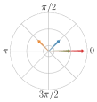
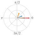
One type of symmetry inherent to complex-valued data is complex-valued scaling ambiguity [18]. For example, consider a complex-valued MRI or SAR signal ${\bf z}$. Due to the nature of signal acquisition, z could be subject to global magnitude scaling and phase offset represented by a complex-valued scalar $s$, thus becoming $s\cdot{\bf z}$.

A complex-valued classifier takes input ${\bf z}$ and ideally should focus on discriminating among instances from different classes, not on the instance-wise variation $s\cdot{\bf z}$ caused by complex-valued scaling. Formally, function $f$ is called complex-scale invariant if $f(s\cdot\mathbf{z})=f(\mathbf{z})$ and called complex-scale equivariant if $f(s\cdot\mathbf{z})=s\cdot f(\mathbf{z})$.

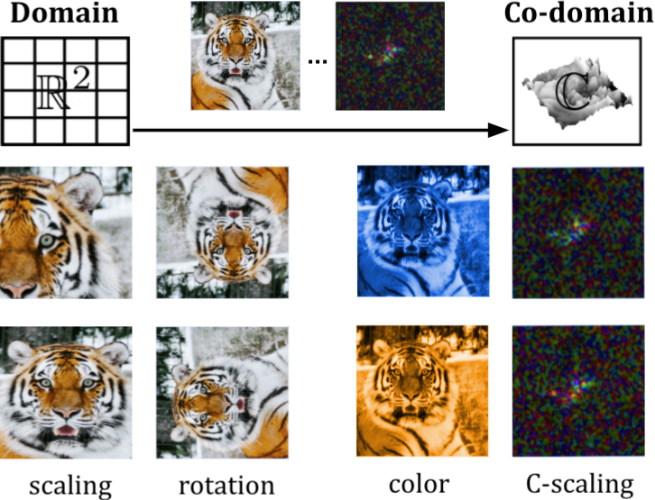
We distinguish two types of image transformations, viewing an image as a function defined over spatial locations. Complex-valued scaling of a complex-valued image is a transformation in the co-domain of the image function, as opposed to a spatial transformation in the domain of the image (Figure 1). Formally, $I:\mathbb{R}^{D}\to\mathbb{C}^{K}$ denotes a complex-valued image of $K$ channels in the $D$-dimensional space, where $\mathbb{R}$ ($\mathbb{C}$) denotes the set of real (complex) numbers. Some common $(D,K)$ are (2,1) for grayscale images, (2,3) for RGB, and $(3,6+)$ for diffusion tensor images.

1. Domain transformation $T:\mathbb{R}^{D}\!\to\!\mathbb{R}^{D}$ transforms the spatial coordinates of an image, resulting in a spatially warped image $I(T(x))$, $x\in\mathbb{R}^{D}$. Translation, rotation, and scaling are examples of domain transformations.

2. Co-domain transformation $T^{\prime}:\mathbb{C}^{K}\to\mathbb{C}^{K}$ maps the pixel value to another, resulting in a color adjusted image $T^{\prime}(I(x))$, $x\in\mathbb{R}^{D}$. Complex-valued scaling and color distortions are examples of co-domain transformations.

Complex-valued scaling thus presents not only a practical setting but also a case study for co-domain transformations.

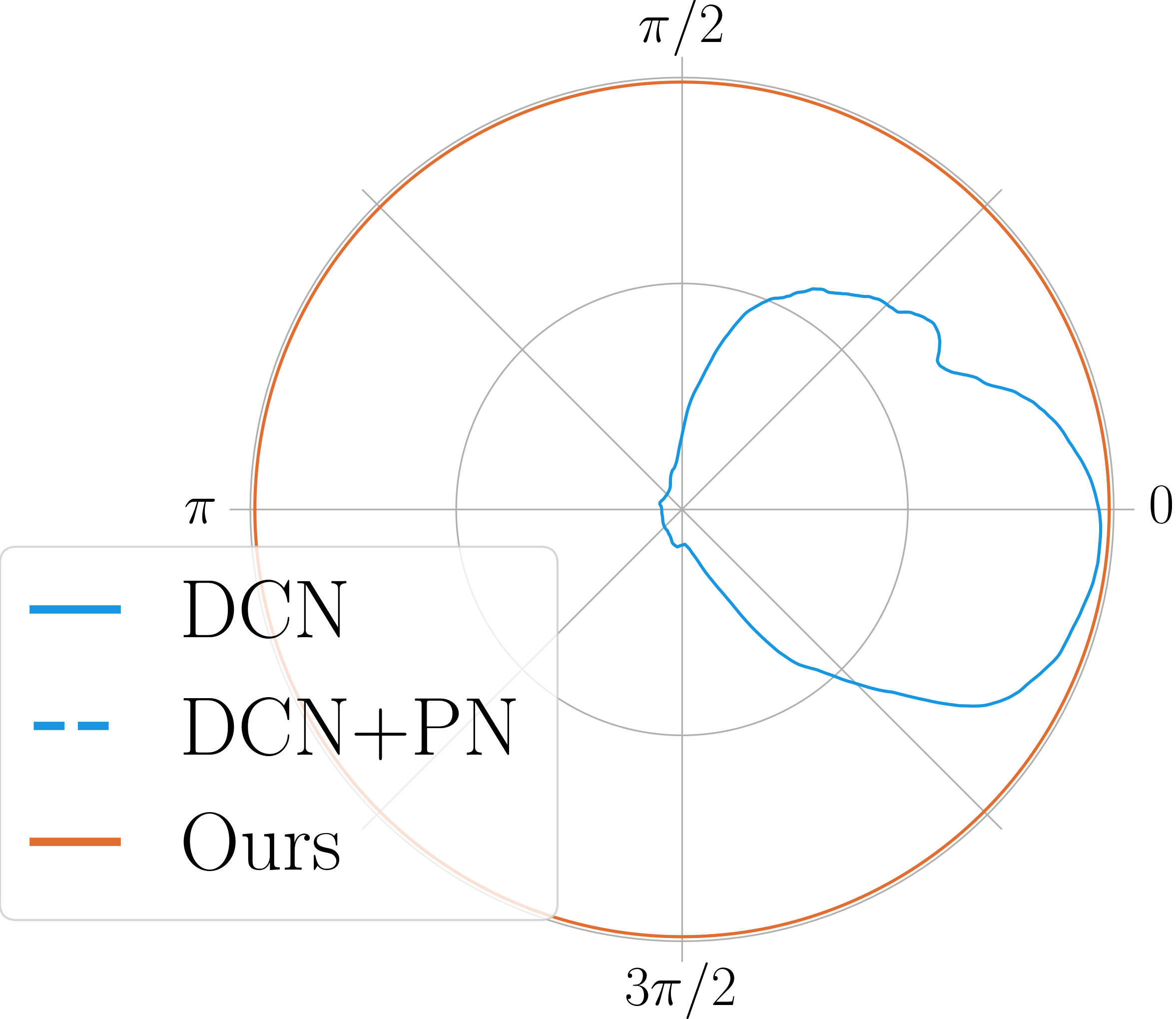
Existing complex-valued deep learning methods such as DCN [16] are sensitive to complex-valued scaling (Fig 2(b)). A pre-processing trick to remove such scaling ambiguity is to simply normalize all the pixel values by setting their average phase to $0$ and magnitude to $1$, but this process introduces artifacts when the phase distribution varies greatly with the content of the image (Figure 2(g)). SurReal [18] applies manifold-valued deep learning to complex-valued data, but this framework only captures the manifold aspect and not the complex algebra of complex-valued data. Thus, a more general, principled method is needed. We propose novel layer functions for complex-valued deep learning by studying how they preserve co-domain symmetry. Specifically, we study whether each layer-wise transformation achieves equivariance or invariance to complex-valued scaling.

Our contributions: 1) We derive complex-scaling equivariant and invariant versions of common layers used in computer vision pipelines. Our model circumvents the limitations of SurReal [18] and scales to larger models and datasets. 2) Our experiments on MSTAR, CIFAR 10, CIFAR 100, and SVHN datasets demonstrate a significant gain in generalization and robustness. 3) We introduce novel complex-valued encodings of color, demonstrating the utility of using complex-valued representations for real-valued data. Complex-scaling invariance under our LAB encoding automatically leads to color distortion robustness without the need for color jitter augmentation.

2 Related Work

Complex-Valued Processing: Complex numbers are ubiquitous in mathematics, physics, and engineering [19, 10, 20]. Traditional complex-valued data analysis involves higher-order statistics [21, 22]. [11] demonstrates higher representational capacity of complex-valued processing on the XOR problem. [23] proposes a sparse coding layer utilizing complex basis functions. [24] proposes a biologically meaningful complex-valued model. [25, 26] encodes data features in a complex vector and learns a metric for this embedding. [15] applies complex-valued neural networks to MRI image reconstruction. [27] investigates the role of critical points in complex neural networks. [28] demonstrates that complex networks have smaller generalization error than real-valued, and offers an overview of their convergence and stability. We refer the reader to [16] for a more detailed account of complex-valued deep learning.

Transformation Equivariance/Invariance: An important line of work [5, 6, 29, 30] aims to develop convolutional layers equivariant to domain transformations like rotation/scaling. [6] introduces a principled method for producing group-equivariant layers for finite groups. [5] extends this work to Lie groups on continuous data. [31] uses circular harmonics to produce deep neural networks equivariant to rotation and translation. [32] attempts to produce a general theory of group-equivariant CNNs on the Euclidean space and the sphere. [33] further extends the framework to local gauge transformations on the manifold. This class of methods is well-suited for domain transformations. However, complex-valued scaling is a co-domain transformation, and these methods are not applicable. [7] generalizes neurons to $\mathbb{R}^{3}$ vectors with 3D rotations as a co-domain transformation, introducing rotation-equivariant layers for point-clouds. In contrast, our method handles both the complex algebra and the geometry of complex-valued scaling.

Complex-Valued Scaling: Despite the increasing research interest in complex-valued neural networks, the problem of effectively dealing with complex-scaling ambiguity remains open. [16, 34, 35, 36] propose an extension of real neural architectures to the complex field by redefining basic building blocks such as complex convolution, batch normalization, and non-linear activation functions. However, these methods are not robust against complex-valued scaling. SurReal [18] tackles the problem of complex-scale invariance by adopting a manifold-based view of complex numbers. It models each complex number as an element of a manifold where complex-scaling corresponds to translation and uses tools from manifold-valued learning to create complex-scale invariant models. This results in better generalization to unseen complex-valued data with leaner models. However, the SurReal framework is restrictive (Sec. 3.1), and the complex-valued processing is forced to be linear (Sec. 3.2), preventing SurReal from scaling to large datasets (Table 1).

3 Equivariance and Invariance for Complex-Valued Deep Learning

3.1 Equivariant Convolution

In contrast to domain transformations which group-specific convolution layers for equivariance [5, 6], any linear layer is equivariant to complex-valued scaling: For a linear function $L:\mathbb{C}^{n}\to\mathbb{C}^{n}$ with an input vector $x\in\mathbb{C}^{n}$ and complex scalar $s\in\mathbb{C}$, $L(s\cdot x)=s\cdot L(x)$. While a bias term is useful in real-valued neural networks, it turns the convolution layer into an affine function, destroying complex-scale equivariance. Thus, we remove the bias term from the complex-valued convolution used in DCN [16], restoring its equivariance. Additionally, we use Gauss’ multiplication trick to speed up the convolution by $25\%$.

Given a complex-valued input feature map $\mathbf{z}=\mathbf{a}+i\mathbf{b}\in\mathbb{C}^{C\times H\times W}$ with $C$ channels and $H\times W$ pixels, and given a convolutional filter of size $K\times K$ with weight $\mathbf{W}=\mathbf{X}+i\mathbf{Y}\in\mathbb{C}^{C\times C\times K\times K}$, we define the Complex-Scale Equivariant Convolution as:

$$\operatorname{Econv}(\mathbf{z};\mathbf{W})=\mathbf{W}*\mathbf{z}= \ (\mathbf{X}+i\mathbf{Y})*(\mathbf{a}+i\mathbf{b})$$

$$= \ \mathbf{t_{1}}-\mathbf{t_{2}}+i(\mathbf{t_{3}}-\mathbf{t_{1}}-\mathbf{t_{2}})$$

where $\mathbf{t_{1}}=\mathbf{X}\ *\ \mathbf{a}$, $\mathbf{t_{2}}=\mathbf{Y}\ *\ \mathbf{b}$, $\mathbf{t_{3}}=(\mathbf{X}+\mathbf{Y})\ *\ (\mathbf{a}+\mathbf{b})$, and $\mathbf{X}*\mathbf{a}$ represents the convolution operation on $\mathbf{a}$ with weight $\mathbf{X}$. In contrast, SurReal uses weighted Frechet Mean (wFM), a restricted convolution where the weights are constrained to be real-valued, positive, and to sum to $1$. This restrictive formulation drastically reduces accuracy.

3.2 Equivariant Non-Linearity

Non-linear activation functions such as ReLU are necessary to construct deep hierarchical representations. For complex-valued data, several alternatives have been studied [16, 36, 37, 18]. $\mathbb{C}$ReLU, the most prominent example, computes ReLU independently on the real and imaginary parts of the input. Tangent ReLU (TReLU) [18] uses the polar representation, thresholding both magnitude and phase.

However, these non-linearities are not complex-scale equivariant. DCN [16] uses $\mathbb{C}$ReLU, failing to be robust against complex-scaling. SurReal does not use non-linearities in its complex-valued stages (see Tables I & II in [18]). SurReal’s complex processing is thus fully linear, preventing it from scaling to large datasets (See Table 1).

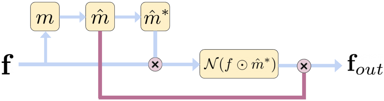
We introduce a general class of equivariant non-linearities which act on the relative phase information between features (Fig. 3). Given a complex-valued input feature map $\mathbf{f}\in\mathbb{C}^{C\times H\times W}$ with $C$ channels and $H\times W$ pixels, and given any non-linear activation function $\mathcal{N}:\mathbb{C}\to\mathbb{C}$, we compute an equivariant version of $\mathcal{N}$ (denoted $\mathcal{E}\{\mathcal{N}\}$) as:

$$\mathbf{f}_{out}=\mathcal{E}\{\mathcal{N}\}(\mathbf{f})=\mathbf{\hat{m}}\odot\mathcal{N}(\mathbf{f}\odot\mathbf{\hat{m}^{*}})$$ (1)

where $\odot$ denotes element-wise multiplication, $\hat{\mathbf{m}}^{*}$ denotes the complex conjugate of $\hat{\mathbf{m}}$, and $\mathbf{\hat{m}}$ is the normalized per-pixel mean feature:

$$\mathbf{m}(x,y)=\frac{1}{C}\sum_{c=1}^{C}\mathbf{f}(c,x,y);\ \mathbf{\hat{m}}(x,y)=\frac{\mathbf{m}(x,y)}{|\mathbf{m}(x,y)|}$$ (2)

The normalized mean $\mathbf{\hat{m}}$ is equivariant to input phase and invariant to input magnitude. As a result, the product $\mathbf{f}\odot\mathbf{\hat{m}^{*}}(x,y)$ is invariant to phase and equivariant to magnitude. If $\mathcal{N}$ is equivariant to magnitude (e.g., $\mathbb{C}$ReLU), the overall layer $\mathcal{E}\{\mathcal{N}\}$ is equivariant to both phase and magnitude.

Figure 3: Our equivariant non-linearity, $\mathcal{E}\{\mathcal{N}\}$, works in four stages. We compute the channel mean $m$ of the input feature $f$ and normalize it to retain only phase information. This normalized mean vector $\hat{m}$ is equivariant to input phase. We multiply $f$ by $\hat{m}^{*}$ to cancel the input phase, resulting in a phase-invariant feature $f\odot\hat{m}^{*}$. We feed this feature to the non-linearity $\mathcal{N}$ and multiply by $\hat{m}$ to restore the previously cancelled input phase. The result is equivariant in phase and also equivariant in magnitude if $\mathcal{N}$ is.

3.3 Equivariant Pooling

In real-valued networks, max-pooling selects the largest activations from a set of neighboring activations. However, for complex numbers, this scheme selects for phase $0\leq\phi\leq\frac{\pi}{2}$ over other phases even though they may encode similar salience. Additionally, this process destroys complex-scale equivariance. To remove this dependence on phase, we select the pixels with the highest magnitude. The result is equivariant to both magnitude and phase.

3.4 Phase-Equivariant Batch Normalization

We follow Deng et. al [7], computing Batch Normalization [38] only on the magnitude of each complex-valued feature, thus preserving the phase information. Given an input feature map $\mathbf{f}\in\mathbb{C}^{C\times H\times W}$, we compute:

$$\mathbf{f}_{BN}=BN(|\mathbf{f}|)\odot\frac{\mathbf{f}}{|\mathbf{f}|}$$ (3)

where $BN$ refers to real-valued BatchNorm and $\odot$ is elementwise multiplication. This layer is equivariant to phase and invariant to input magnitude.

3.5 Complex-Valued Invariant Layers

In order to produce invariant complex-valued features, we introduce the Division Layer and the Conjugate Multiplication Layer. Given two complex-valued features $\mathbf{z_{1}},\mathbf{z_{2}}\in\mathbf{C}^{H\times W}$, we define:

$$\text{Div}({\bf z_{1},z_{2}})= \ \frac{|\mathbf{z_{1}}|}{|\mathbf{z_{2}}|+\epsilon}\exp\{i(\measuredangle{\mathbf{z_{1}}}-\measuredangle{\mathbf{z_{2}}})\}$$ (4)

$$\text{Conj}({\bf z_{1},z_{2}})= \ \mathbf{z_{1}}\mathbf{z_{2}^{*}}$$ (5)

In practice, the denominator for division can be small, so we offset the magnitude of the denominator by $\epsilon=10^{-7}$.

While the division layer induces invariance to all complex-valued scaling, the conjugate layer only induces invariance to phase. This layer also captures some second-degree interactions similar to a bilinear layer [39]. In contrast to our layers which capture relative phase and magnitude offsets of input features, SurReal’s Distance Layer achieves invariance by extracting real-valued distances between features, discarding rich complex-valued information in the process.

Figure 4: Our Division Layer is complex-scale invariant, and preserves more information than the Distance Transform [18]. Consider 4 complex numbers (colored dots) and the reference (black dot). Complex-scaling changes the orientation and size of the trapezoid. While the manifold distances [18] from the black dot to the colored dots are identical, the Division Layer output is invariant and distinct for each dot (the same colored dots around $0^{\circ}$).

3.6 Generalized Tangent ReLU

In practice, TReLU slows down convergence compared to $\mathbb{C}$ReLU. We remedy this through three modifications: a) a learned complex-valued scaling factor for each input channel, enabling the layer to adapt to input magnitude and phase, b) hyperparameter $r$ to control the magnitude threshold. Notably, $r=0$ produces a phase-only version of TangentReLU, which is equivariant to input magnitude, and c) learned scaling constant for the output phase of each channel, allowing the non-linearity to adapt the output phase distribution. Our proposed method generalizes TReLU both as a transformation and as a thresholding function. It is defined as:

$$\operatorname{GTRelu}(\mathbf{x};r,c,\omega)=\max(r,|c\cdot\mathbf{x}|)exp\{i\omega\measuredangle{(c\cdot\mathbf{x}})_{+}\}$$

where $x\in\mathbb{C}$ is a scalar input, $r\in\mathbb{C}$ is the threshold parameter, $c\in\mathbb{C}$ and $\omega\in\mathbb{R}$ are learned scaling factors, and $x_{+}=ReLU(x)=max(x,0)$ (Figure 5).

(a) Input features

(b) Scaling factor

(c) Thresholding

(d) Phase-scaling

Figure 5: Our Generalized Tangent ReLU transforms the input in three stages: (a) given input complex vectors, it multiplies each channel with a learned scaling factor, (b) thresholds the input magnitude and phase with hyperparameter $r$, and (c) scales the phase to adapt the output distribution.

3.7 Complex Features $\to$ Real-Valued Outputs

In order to produce real-valued outputs from complex-valued features, we propose using feature distances, which are commonly used for prototype-based classification. Given a complex-valued feature vector $\mathbf{f}\in\mathbf{C}^{D}_{emb}$ with embedding dimension $D_{emb}$, we compute the distance of $\mathbf{f}$ to every class prototype vector $\mathbf{p_{i}}\in\mathbf{C}^{D}_{emb}$. The input is then classified as belonging to the class of the nearest prototype $\mathbf{p_{i}}$. Formally, we define the logits returned by the network as the negative distance to the prototype scaled by a learned distance scaling factor $\alpha\in\mathbf{R}^{+}$. Formally, the i-th logit $L_{i}\in\mathbf{R}$ is:

$$L_{i}=-\alpha\cdot d\left(\mathbf{f},\mathbf{p_{i}}\right)$$ (6)

Since the features are complex-valued, a suitable metric is the manifold distance (equivalent to [18]):

$$d\left({z}_{1},{z}_{2}\right)\!=\!\sqrt{\big{(}\ln{|z_{1}|}-\ln{|z_{2}|}\big{)}^{2}+\operatorname{arc}(\measuredangle{z_{1}},\measuredangle{z_{2}})^{2}}$$ (7)

where $z_{1},z_{2}\in\mathbb{C}$. It amplifies the effect of phase differences which would otherwise be suppressed by large variations in magnitude. Alternatively, a simple metric is the Euclidean distance. In practice, we use BatchNorm on the input features before computing distances to accelerate convergence.

Invariant Distance Layer: Similar to the Distance Layer [18], this layer can be made complex-scale invariant by multiplying the prototypes with an equivariant feature map:

$$L_{i}=-\alpha\cdot d\left(\mathbf{f},\mathbf{p_{i}}\odot\mathbf{m}\right)$$ (8)

where $\mathbf{m}$ is the mean activation averaged over channels.

3.8 Composing Equivariant and Invariant Layers

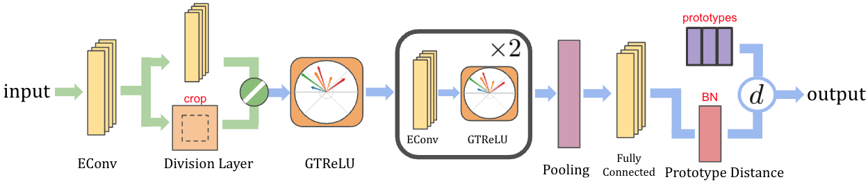
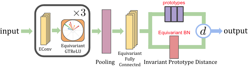
We introduce two patterns of model composition based on our proposed layers. Type I models use a complex-valued invariant layer in the early stages to achieve complex-scale invariance, and Type E models use equivariant layers throughout the model, retaining more information.

Type I: These models consist of a complex-valued invariant layer (Division/Conjugate) in the early stages, producing complex-scale invariant features which can be used by later stages without any architectural restrictions.

Type E: These models use equivariant layers throughout the network, relying on Equivariant convolutions, non-linear activations, and pooling layers, followed by a invariant distance layer to obtain invariant predictions. This model preserves the phase information through equivariant layers and thus can typically achieve higher accuracy. However, this class of models is less flexible than Type I.

Model Type I
Model Type E

Figure 6: Our CIFARnet models demonstrate two methods of constructing complex-scale invariant models. Green arrows represent equivariant features, and blue arrows represent invariant features. top: Type I architecture uses a Division Layer in early stages, producing complex-scale invariant features which can be used with any following layers. bottom: Type E uses equivariant layers throughout the network, retaining phase information until the final Invariant Prototype Distance Layer. This class of models is more restrictive but can achieve higher accuracy (See Table 1) as a consequence of retaining more information.

4 Complex-Valued Color Encodings

Spectral representations like the Fourier Transform are invaluable for analyzing real-valued signals. However, their usefulness in convolutional neural networks is undermined by the fact that CNNs are designed to tackle spatially homogeneous and translation-invariant domains, while Fourier data is neither. We propose two complex-valued color encodings which capture hue shift and channel correlations respectively, demonstrating the utility of complex-valued representations for real-valued data.

Our first so-called "Sliding" encoding takes an $[R,G,B]$ image and encodes it with two complex-valued channels:

$$[R,G,B]\rightarrow\left[R+iG,G+iB\right]$$ (9)

The complex phase in this encoding corresponds to the ratio of R, G, B values, so the phase in this encoding captures the correlation between the adjacent color channels.

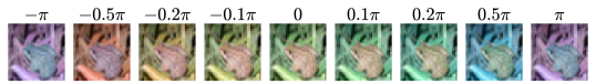
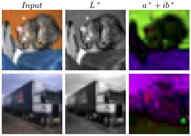
Our second proposed encoding uses $L^{*}a^{*}b^{*}$, a perceptually uniform color representation with luminance represented by the $L$ channel and chromaticity by the $a$ and $b$ channels. [40] uses this color space for image colorization. We use it to represent color as a two-channel, complex-valued representation, with the first channel containing the luminance ($L^{*}$ channel), and the second channel containing chromaticity ($a^{*}$ and $b^{*}$ channels) as $a^{*}+i\,b^{*}$ (Figure 2(c)):

$$[R,G,B]\rightarrow\left[L^{*},a^{*}+ib^{*}\right]$$ (10)

Color distortions as co-domain transformations: Color distortion can be approximated with complex-valued scaling of our LAB color representation (Figure 2(a)). A complex-scale invariant network is thus automatically robust to color distortions without the need for data augmentation.

5 Experiments

We conduct three kinds of experiments: Accuracy: 1) Classification of naturally complex-valued images, 2) real-valued images with real and complex representations; Robustness against complex scaling and color distortion; Generalization: 1) Bias-variance analysis, 2) generalization on smaller training sets, 3) Feature redundancy analysis.

5.1 Complex-Valued Dataset: MSTAR

MSTAR contains 15,716 complex-valued synthetic aperture radar (SAR) images divided into 11 classes [41]. Each image has one channel and size $128\times 128$. We discard the last "clutter" class and follow [42], training on the depression angle $17^{\circ}$ and testing on $15^{\circ}$. We train each model on varying proportions of the dataset to evaluate the accuracy and generalization capabilities of each model.

SurReal: We replicate the architecture described in Table 1 of [18]. Since the paper does not mention the learning rate, we use the same learning rate and batch size as our model. DCN: We use author-provided code, creating a complex ResNet with $\mathbb{C}$ReLU and 10 blocks per stage. By default, this model accepts $32\times 32$ images, so we append $2\times[\textit{ComplexConv},\textit{ComplexBatchNorm}]$ with stride $2$ to downsample the input. The model is trained for 200 epochs using SGD with batch size $64$ and the learning rate schedule in [16]. We select the epoch with the best validation accuracy. Real-valued baseline: We use a 3-stage ResNet with 3 layers per residual block and convert the complex input into two real-valued channels.

CDS: We use a Type I model based on SurReal [18]. We extract equivariant features using an initial equivariant block containing EConv, Eq. GTReLU, Eq. MaxPool layers, and then obtain complex-scale invariant features by using a Division Layer. These features are then fed to a real-valued ResNet. For more details about every model, please refer to supplementary materials.

Training: We optimize both SurReal and CDS models using the AdamW optimizer [43, 44] with learning rate $10^{-3}$, momentum $(0.9,0.99)$, weight decay $0.1$, and batch size $256$ for $2.5\times 10^{5}$ iterations . We validate every $1000$ steps, picking the model with the best validation accuracy.

(a) Scaling Laws for MSTAR [45]

(b) Class-wise Bias and Variance for CIFAR10 [46]

(c) Filter similarity histogram for conv2

Figure 7: Our model generalizes across various dataset sizes, has lower bias and variance, and avoids learning redundant filters. (a): We produce trend curves (similar to [45]) for the MSTAR accuracy table (Table 2). Our method has the lowest test error for measured dataset sizes, a trend that is predicted to scale to even smaller sizes. (b): We followed [46] for CIFAR10 models with LAB encoding. Classes are ordered in ascending order of bias for our model. Our model consistently shows the lowest bias for each class, and the lowest variance for 9 out of 10 classes, indicating overall superior generalization ability. (c): Filter similarity histogram from conv2 layer of each CIFARnet model, following [47]. Our distribution mean is closest to $0$, indicating our method achieves the least redundant filters.

Method	# Param	CIFAR10			CIFAR100			SVHN
		RGB	LAB	Sliding	RGB	LAB	Sliding	RGB	LAB	Sliding
DCN [16]	66,858	65.17	58.64	63.83	32.52	27.36	28.87	85.26	84.43	87.44
SurReal [18]	35,274	50.68	53.02	54.61	23.57	25.97	26.66	80.51	53.48	80.79
Real-valued CNN	34,282	64.43	63	63.43	31.93	31.72	31.93	87.47	84.93	87.37
Ours (Type-I)	24,241	69.23	67.17	68.7	36.92	37.81	38.51	89.39	88.86	90.25
Ours (Type-E)	25,745	68.48	67.58	69.19	41.83	39.55	42.08	77.19	74.21	88.39

Table 1: Our models outperform the baselines’ CIFARnet versions on real-valued datasets. Type-I model performs better on easier datasets like SVHN, and Type-E performs better on difficult datasets like CIFAR100. In contrast, SurReal does not scale to large datasets.

5.2 Real-valued Datasets: CIFAR10/100, SVHN

Datasets: CIFAR10 [48] (and CIFAR100) consists of 10 (100) classes containing 6000 (600) images each. Both CIFAR10 and CIFAR100 are partitioned into 50000 training images and 10000 test images. SVHN [49] consists of house number images from Google Street View, divided into 10 classes with $73,257$ training digits and $26,032$ testing digits.

Models: To ensure equal footing for each model, all networks in this experiment are based off CIFARNet, i.e., 3 Convolution Layers (stride 2) and 2 fully connected layers. We also replace average pooling with a depthwise-separable convolution as a learnable pooling layer. All models are optimized with AdamW [43, 44] using momentum $(0.99,0.999)$, for $5\times 10^{4}$ steps with batch size $256$, learning rate $10^{-3}$, weight decay $0.1$, and validated every $1000$ iterations. DCN: We use ComplexConv for convolutions and $\mathbb{C}$ReLU as the non-linearity. We do not use Residual Blocks or Complex BatchNorm from [16] to ensure fairness. SurReal: We use wFM for convolutions and use Distance Transform after Layer 3 to extract invariant real-valued features. Real-Valued CNN: We use the CIFARNet architecture, converting each complex input channel into two real-valued channels. CDS: We evaluate two models: Type I: We use EConv for convolutions and GTReLU ($r=0$) for non-linearity. We use a Division layer after the first Econv to achieve invariance. The final fully-connected layer is replaced with Prototype Distance layer to predict class logits (Figure 6). Type E: We use Econv for convolutions and Equivariant GTReLU for non-linearity. The final FC layer is replaced with Invariant Prototype Distance layer to predict logits (Figure 6), and the prototype distance inputs are normalized with Equivariant BatchNorm to preserve equivariance.

CDS-Large: We train a $1.7M$ parameter Type I model on CIFAR 10 with LAB encoding, and compare it against equivalently sized DCN (WS with $\mathbb{C}$ReLU from [16]). CDS-Large is based on the simplified 4-stage ResNet provided by Page et al. [50] for DAWNBench [51]. We use the conjugate layer after the first Econv to get complex-scale invariant features and feed them to the Complex ResNet. Like DCN, we optimize the model using SGD with horizontal flipping and random cropping augmentations with a varying learning rate schedule (see supplementary material for more details).

5.3 Model Performance Analysis

Accuracy and scalability: Our approach achieves complex-scale invariance of manifold-based methods while retaining high accuracy and scalability. On MSTAR, our model beats the baselines across a diverse range of splits with less than half the parameters used by SurReal (Table 2). On the smallest training split ($5\%$ training data), our model shows a gain of $19.7\%$ against DCN and real-valued CNN and $8.4\%$ against SurReal. On the largest split ($100\%$ training data), our model beats real-valued CNN by $29.2\%$, DCN by $7\%$, and SurReal by $1.2\%$, demonstrating our advantage across an extensive range of dataset sizes.

Model	# Params	5%	10%	50%	90%	100%
Real	33,050	47.4	46.6	60.6	73	66.9
SurReal [18]	63,690	61.1	68	90.3	95.6	94.9
DCN [16]	863,587	49.8	47	81.9	89.1	89.1
Ours	29,536	69.5	78.3	91.3	95.2	96.1

Table 2: Our method achieves the best accuracy and generalization with the fewest parameters. We report accuracy on varying proportions of MSTAR training data. The performance gap is wider for smaller train-sets, with Real-CNN and DCN failing to generalize.

On CIFAR10, CIFAR100, and SVHN under different encodings, our models obtain the highest accuracy across every setting (Table 1). Unlike SurReal, our model scales to these large classification datasets while retaining complex-scale invariance. For the complex-valued color encodings, which require precise processing of phase information, our model consistently beats baselines by $4\%$-$8\%$. These results highlight the advantage of our approach for precise complex-valued processing across a variety of real-valued datasets.

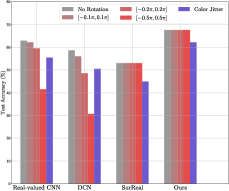
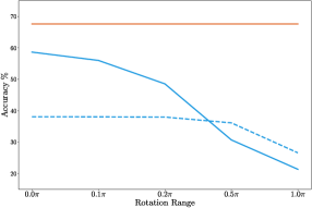
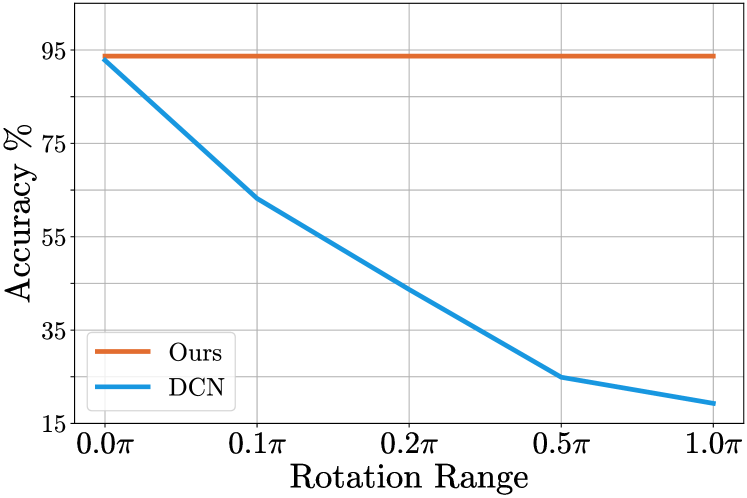
Phase normalization and color jitter: A natural pre-processing trick to address complex-scaling invariance is to compute the average input phase $\hat{\phi}$ and to scale the input by $e^{-\iota\hat{\phi}}$ to cancel it. We test this approach by applying random complex-valued scaling with different rotation ranges and comparing DCN’s accuracy with and without phase normalization against our method (Figure 2(g)). When the input phase distribution is simple (e.g., phase set to 0), phase normalization successfully protects DCN against complex-valued scaling. However, for complicated phase distributions such as LAB encoding, this method fails. Our method succeeds in both situations, and this robustness transfers to the color jitter (as used by [17], see Figure 2(f)). Our model is more robust against color jitter without data augmentation.

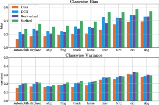
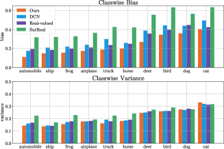
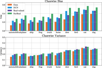
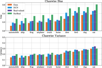
Bias and variance analysis: While model accuracy across different datasets is useful, a better measure for the generalization of supervised models is the bias-variance decomposition. We follow [46]: given model $f$, dataset $D$, ground truth $Y$ and instance $x$, [46] defines the bias-variance decomposition of the prediction error (per instance) as:

$$\operatorname{Error}(x;f) =E\left[(f(x;D)-Y)^{2}\right]$$ (11)

$$=\operatorname{Bias}(x;f)+\operatorname{Var}(x;f)+\text{R}(x)$$ (12)

where bias measures the accuracy of the predictions with respect to the ground-truth, variance measures the stability of the predictions, and $R$ denotes the irreducible error. Using the 0-1 loss $\mathcal{L}_{0-1}$, [46] calculates the bias and variance terms (per instance per model) for the classification task as such:

$$\operatorname{Bias}(x;h) =\mathcal{L}_{0-1}\left(y_{m};t\right)$$ (13)

$$\operatorname{Var}(x;h) =\frac{1}{n}\sum_{k=1}^{n}\mathcal{L}_{0-1}\left(y^{(k)};y_{m}\right)$$ (14)

where $y_{m}$ is the mode or the main prediction. We compute this metric for each instance, averaging bias and variance over classes. Compared on CIFAR10 with LAB encoding, our model achieves the lowest bias among all classes and the lowest variance among 9 out of 10 classes (Figure 7).

Method	#Params	%Acc
DCN [16]	1.7M	92.8
Ours	1.7M	93.7

(a) CIFAR10 LAB accuracy for large models

(b) Robustness Curve for large models

Figure 8: Our model beats DCN while additionally achieving complex-scale invariance. a) We train DCN and CDS on CIFAR10 with the LAB encoding, achieving higher accuracy. This result is consistent with (Table 1), with smaller margin due to the larger capacity of big models. b) DCN is susceptible to complex-valued scaling. Similar to Figure 1g, we plot average accuracy under different rotation ranges. DCN accuracy degrades under complex-valued scaling, while our method is robust.

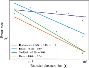
Generalization from less training data: [45] derives empirical trends for scaling of language models under different conditions, including the overfitting regime where the training set is small compared to parameters. We produce similar trend curves for the MSTAR test results by fitting linear regression curves to log accuracy and dataset size reported in Table 2. We plot the results in Figure 7. The extrapolated least-squares linear fit suggests our model might continue to generalize better on yet smaller datasets.

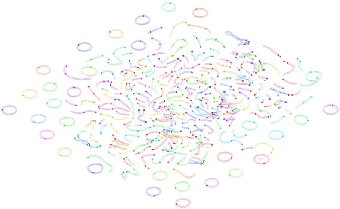
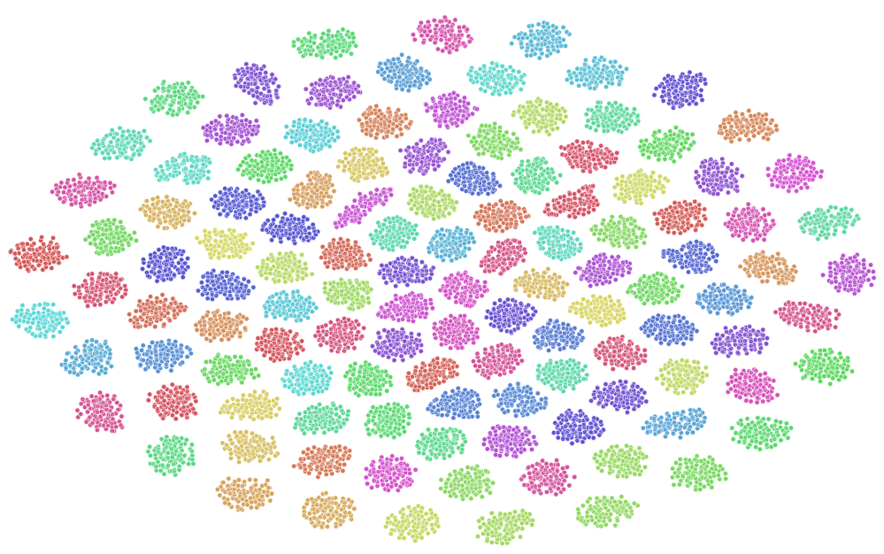
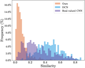
Feature redundancy comparison: [47] shows that common CNN architectures learn highly correlated filters. This increases model size and reduces the ability to capture diversity. We follow [47], measuring correlations between guided backpropagation maps of different filters in layer $2$ for each model on CIFAR10 with the LAB encoding. We find that our model displays the highest filter diversity. This observation is consistent with higher test accuracy, lower bias and variance, and leaner models from previous experiments.

Scaling to large models: Small models are essential for applications such as edge computing, thus motivating leaner models (Table 1 and 2). However, the best models on large real-valued datasets, like ViT-H/14 [52] with $99.5\%$ test accuracy on CIFAR10, have millions of parameters. We test the scalability of our approach by comparing CDS-Large with a DCN model of equivalent size on CIFAR10 with LAB encoding (Table 8(a)). While we focus on leaner complex-scale invariant models, our method beats DCN while additionally achieving complex-scale invariance even for large models. This observation is consistent with our results for small models (Table 1), showing the effectiveness of our method for diverse model sizes.

Summary: We analyze complex-scaling as a co-domain transformation and derive equivariant/invariant versions of commonly used layers. We also present novel complex encodings. Our approach combines complex-valued algebra with complex-scaling geometry, resulting in leaner and more robust models with better accuracy and generalization.

Acknowledgements: The authors gratefully acknowledge DARPA, AFRL, and NGA for funding various applications of this research. We also thank Matthew Tancik, Ren Ng, Connelly Barnes, and Claudia Tischler for their thoughtful comments.

6 Supplementary Material

Table of contents:

1. Extensive bias-variance evaluation, including plots for both LAB and RGB encodings.

2. Limitations of wFM as a convolutional layer in CNNs.

3. Ablation tests

4. Architecture details for models used in our experiments.

6.1 Bias-Variance Evaluation

In this section, we run extensive evaluations for bias and variance on each encoding for the CIFAR10 dataset with CIFARNet models (Figure 9). In each case, our model (Type E) achieves the lowest bias for each class. We also achieve the lowest variance for 8 (out of 10) classes for RGB, 9 classes for LAB, and all classes for the Sliding encoding. Our overall bias and variance are the lowest of all models, indicating higher generalization ability.

(a) RGB encoding

(b) LAB encoding

(c) Sliding encoding

Figure 9: Our method demonstrates lowest overall bias and variance on CIFAR10. We followed [46] for CIFAR10 models with RGB encoding. Classes are ordered in ascending order of bias for our model. Our model consistently shows the lowest bias for each class in every encoding, and lowest variance in 8, 9, and 10 out of 10 classes with RGB, LAB, and Sliding encodings respectively.

6.2 Limitations of wFM

We demonstrate the theoretical and empirical limitations of wFM. From a theoretical perspective, we show that wFM using the Manifold Distance Metric of SurReal processes magnitude and phase separately and is thus unable to process the joint distribution. Our experiments show that in practice, wFM results in a significant loss in accuracy compared to real-valued and complex-valued convolutional filters.

Decomposability: We discuss the weighted-Fréchet Mean for complex-valued neural networks and show that the magnitude and phase computations are decoupled. wFM is defined as the minimum of weighted distances to a given set of points. In specific cases (like the Euclidean distance metric), closed-form solutions (like the euclidean weighted mean) exist, but there is no general closed-form solution.

Given $\left\{\mathbf{z}_{i}\right\}_{i=1}^{K}\subset\mathbf{C}$ and $\left\{w_{i}\right\}_{i=1}^{K}\subset(0,1]$ with $\sum_{i}w_{i}=1$ and $b\in\mathbf{R}$, we aspire to compute:

$$\arg\min_{\mathbf{m}\in\mathbf{C}}\sum_{i=1}^{K}w_{i}d^{2}\left(\mathbf{z}_{i},\mathbf{m}\right)$$ (15)

Using the Manifold distance metric, the expression reduces to:

$$\arg\min_{\mathbf{m}\in\mathbf{C}}\sum_{i=1}^{K}w_{i}\left((\ln|\mathbf{z}_{i}|-\ln|\mathbf{m}|)^{2}+\operatorname{arc}^{2}(\mathbf{z_{i}},\mathbf{m})\right)$$ (16)

Note that the objective is a sum of $\log|\mathbf{z}_{i}|-\log|\mathbf{m}|)^{2}$ and $\operatorname{arc}^{2}(\mathbf{z_{i}},\mathbf{m})$, where the first objective depends only on the magnitude of $\mathbf{m}$, and the second objective depends only on the phase of $\mathbf{m}$. Thus, the magnitude and phase can be solved independently of each other. The first can be further simplified:

$$r^{*}=\arg\min_{r\in\mathbf{R}}\sum_{i=1}^{K}w_{i}(\log|\mathbf{z}_{i}|-r)^{2}$$ (17)

$$\implies r^{*}=\sum_{i=1}^{K}w_{i}.\log|\mathbf{z}_{i}|$$ (18)

$$\implies\log|m^{*}|=\sum_{i=1}^{K}w_{i}.\log|\mathbf{z}_{i}|$$ (19)

Thus, wFM simply computes a weighted sum of log magnitudes and solves a different minimization problem to find the phase. This restricts the representational power of a wFM layer compared to that of a convolution.

wFM experiments: We compare wFM against real-valued and complex-valued convolutions on CIFAR10 using a CIFARnet architecture. We find that the lower representational capacity of wFM leads to significant reductions in accuracy (Table 3).

Layer Type	Params	Acc (%)
Complex	66,858	58.6
Real	34,282	63.4
wFM	42,154	52.2

Table 3: wFM results in significant reductions in accuracy. We train models on CIFAR10 with LAB encoding and tabulate the resulting test accuracy. Compared to a real-valued CNN, wFM results in significantly lower accuracy due to its restricted formulation.

6.3 Ablation tests

In this section, we run ablation tests for our Type I model on CIFAR10 under the LAB encoding to measure the impact of layer choices on final performance. Specifically, we benchmark the Complex Invariant Layer, the Invariant Distance Layer, and different thresholds for the Generalized Tangent ReLU layer (Table 4). We find that the Division layer beats the Conjugate layer in terms of accuracy and that Manifold Distance achieves higher accuracy than our baseline of Euclidean Distance. We also note that among GTReLU thresholds, $r=0.1$ performs the best but is not equivariant to magnitude. We also note that higher thresholds like $r=1$ result in lower accuracy.

Method	Accuracy
Division Layer	67.17
Conjugate Layer	66.73
Euclidean Distance	67.17
Manifold Distance	68.54
GTReLU (r=0)	67.17
GTReLU (r=0.1)	68.14
GTReLU (r=1)	49.15

Table 4: Ablation test results for our Type-I model on CIFAR 10 with LAB encoding. We find that Division Layer, Manifold Distance, and a GTReLU threshold of $r=0.1$ perform the best.

6.4 Architecture Details

In this section, we discuss details of the architectures used in our experiments.

CIFARnet architectures: For CIFARnet architectures, please refer to tables 5-9. Please note that our replication of wFM [18] uses the $(\log mag,sin\theta,cos\theta)$ encoding for the manifold values, and uses the weighted average formulation.

MSTAR architectures: For DCN, please refer to [16], and for the downsampling block, see Table 11. Our SurReal replication is based on Table I in [18], and our model is based on the SurReal architecture (see Table 13). We use the same real-valued ResNet as the real-valued baseline (see Table 12). In order to pass the complex-valued features into the real-valued ResNet, we convert complex features to real-valued using the $(\log mag,sin\theta,cos\theta)$ encoding, treating each as a separate real-valued channel (resulting in 15 real-valued channels from 5 complex-valued channels).

CDS-Large: For the model architecture, please see Table 10. We train this model with SGD, using momentum $0.9$, weight decay constant $5\times 10^{-4}$, using a piece-wise linear learning rate schedule starting at $0.01$, increasing to $0.2$ by epoch $10$, then decreasing to $0.01$ by epoch $100$, $0.001$ by $120$, $0.0001$ by $150$, and staying constant until $200$. To ensure fair comparison, use horizontal flips and random cropping augmentation as used in [16]. All models are implemented in PyTorch [53].

Table 5: SurReal CIFAR Model Architecture

Layer Type	Input Shape	Kernel	Stride	Padding	Output Shape
Complex CONV	$[3,32,32]$	$3\times 3$	2	1	$[16,16,16]$
$G$-transport	$[16,16,16]$	-	-	-	$[16,16,16]$
Complex CONV	$[16,16,16]$	$3\times 3$	2	1	$[32,8,8]$
$G$-transport	$[32,8,8]$	-	-	-	$[32,8,8]$
Complex CONV	$[32,8,8]$	$3\times 3$	2	1	$[64,4,4]$
$G$-transport	$[64,4,4]$	-	-	-	$[64,4,4]$
Distance Layer	$[64,4,4]$	-	-	-	$[64,4,4]$
Average Pooling	$[64,4,4]$	$4\times 4$	-	-	$[64,1,1]$
FC	$[64]$	-	-	-	$[128]$
ReLU	$[128]$	-	-	-	$[128]$
FC	$[128]$	-	-	-	$[10]$

Table 6: DCN CIFAR Model Architecture

Layer Type	Input Shape	Kernel	Stride	Padding	Output Shape
Complex CONV	$[3,32,32]$	$3\times 3$	2	1	$[16,16,16]$
$\mathbb{C}$ReLU	$[16,16,16]$	-	-	-	$[16,16,16]$
Complex CONV	$[16,16,16]$	$3\times 3$	2	1	$[32,8,8]$
$\mathbb{C}$ReLU	$[32,8,8]$	-	-	-	$[32,8,8]$
Complex CONV	$[32,8,8]$	$3\times 3$	2	1	$[64,4,4]$
$\mathbb{C}$ReLU	$[64,4,4]$	-	-	-	$[64,4,4]$
Average Pooling	$[64,4,4]$	$4\times 4$	-	-	$[64,1,1]$
Complex-to-Real	$[64,1,1]$	$4\times 4$	-	-	$[128]$
FC	$[128]$	-	-	-	$[128]$
ReLU	$[128]$	-	-	-	$[128]$
FC	$[128]$	-	-	-	$[10]$

Table 7: Our (Type-E) CIFAR Model Architecture

Layer Type	Input Shape	Kernel	Stride	Padding	Output Shape
Econv	$[3,32,32]$	$3\times 3$	2	1	$[16,16,16]$
Eq. GTReLU	$[16,16,16]$	-	-	-	$[16,16,16]$
Econv	$[16,16,16]$	$3\times 3$	2	1	$[32,8,8]$
Eq. GTReLU	$[32,8,8]$	-	-	-	$[32,8,8]$
Econv	$[32,8,8]$	$3\times 3$	2	1	$[64,4,4]$
Eq. GTReLU	$[64,4,4]$	-	-	-	$[64,4,4]$
Average Pooling	$[64,4,4]$	$4\times 4$	-	-	$[64,1,1]$
Equivariant FC	$[64]$	-	-	-	$[128]$
Invariant Prototype Distance	$[128]$	-	-	-	$[10]$

Table 8: Our (Type-I) CIFAR Model Architecture

Layer Type	Input Shape	Kernel	Stride	Padding	Output Shape
Econv	$[3,32,32]$	$3\times 3$	2	1	$[16,16,16]$
Division Layer	$[16,16,16]$	$3\times 3$	-	1	$[16,16,16]$
GTReLU	$[16,16,16]$	-	-	-	$[16,16,16]$
Econv	$[16,16,16]$	$3\times 3$	2	1	$[32,8,8]$
GTReLU	$[32,8,8]$	-	-	-	$[32,8,8]$
Econv	$[32,8,8]$	$3\times 3$	2	1	$[64,4,4]$
GTReLU	$[64,4,4]$	-	-	-	$[64,4,4]$
Average Pooling	$[64,4,4]$	$4\times 4$	-	-	$[64,1,1]$
Equivariant FC	$[64]$	-	-	-	$[128]$
Prototype Distance	$[128]$	-	-	-	$[10]$

Table 9: 2-Channel Real-Valued CIFAR Model Architecture

Layer Type	Input Shape	Kernel	Stride	Padding	Output Shape
CONV	$[3,32,32]$	$3\times 3$	2	1	$[16,16,16]$
ReLU	$[16,16,16]$	-	-	-	$[16,16,16]$
CONV	$[16,16,16]$	$3\times 3$	2	1	$[32,8,8]$
ReLU	$[32,8,8]$	-	-	-	$[32,8,8]$
CONV	$[32,8,8]$	$3\times 3$	2	1	$[64,4,4]$
ReLU	$[64,4,4]$	-	-	-	$[64,4,4]$
Average Pooling	$[64,4,4]$	$4\times 4$	-	-	$[64,1,1]$
FC	$[64]$	-	-	-	$[128]$
ReLU	$[128]$	-	-	-	$[128]$
FC	$[128]$	-	-	-	$[10]$

Table 10: Our CDS-Large Model Architecture

Layer Type	Input Shape	Kernel	Stride	Padding	Output Shape
Econv	$[3,32,32]$	$3\times 3$	1	1	$[64,32,32]$
Conjugate Layer	$[64,32,32]$	$1\times 1$	-	-	$[64,32,32]$
Econv (Groups=2)	$[64,32,32]$	$3\times 3$	1	1	$[64,32,32]$
ComplexBatchNorm	$[64,32,32]$	-	-	-	$[64,32,32]$
$\mathbb{C}$ReLU	$[64,32,32]$	-	-	-	$[64,32,32]$
Econv (Groups=2)	$[64,32,32]$	$3\times 3$	1	1	$[128,32,32]$
ComplexBatchNorm	$[128,32,32]$	-	-	-	$[128,32,32]$
$\mathbb{C}$ReLU	$[128,32,32]$	-	-	-	$[128,32,32]$
Eq. MaxPool	$[128,32,32]$	$2\times 2$	-	-	$[128,16,16]$
ResBlock(groups=2)	$[128,16,16]$	-	-	-	$[128,16,16]$
Econv (Groups=4)	$[128,16,16]$	$3\times 3$	1	1	$[256,16,16]$
ComplexBatchNorm	$[256,16,16]$	-	-	-	$[256,16,16]$
$\mathbb{C}$ReLU	$[256,16,16]$	-	-	-	$[256,16,16]$
Eq. MaxPool	$[256,16,16]$	$2\times 2$	-	-	$[256,8,8]$
Econv (Groups=2)	$[256,8,8]$	$3\times 3$	1	1	$[512,8,8]$
ComplexBatchNorm	$[512,8,8]$	-	-	-	$[512,8,8]$
$\mathbb{C}$ReLU	$[512,8,8]$	-	-	-	$[512,8,8]$
Eq. MaxPool	$[512,8,8]$	$2\times 2$	-	-	$[512,4,4]$
ResBlock(groups=4)	$[512,4,4]$	-	-	-	$[512,4,4]$
Eq. MaxPool	$[512,4,4]$	$2\times 2$	-	-	$[512,1,1]$
Fully Connected	$[1024]$	-	-	-	$[10]$

Table 11: DCN Down-sampling Block for MSTAR

Layer Type	Input Shape	Kernel	Stride	Padding	Output Shape
Complex CONV	$[1,128,128]$	$3\times 3$	2	1	$[12,64,64]$
ComplexBatchNorm	$[12,64,64]$	-	-	-	$[12,64,64]$
Complex CONV	$[1,64,64]$	$3\times 3$	2	1	$[12,32,32]$
ComplexBatchNorm	$[12,32,32]$	-	-	-	$[12,32,32]$

Table 12: MSTAR Real-valued Model Architecture

Layer Type	Input Shape	Kernel	Stride	Output Shape
CONV	$[2,100,100]$	$5\times 5$	1	$[30,96,96]$
GroupNorm$+$ReLU	$[30,96,96]$	-	-	$[30,96,96]$
ResBlock	$[30,96,96]$	-	-	$[40,96,96]$
MaxPool	$[40,96,96]$	$2\times 2$	2	$[40,48,48]$
CONV	$[40,48,48]$	$5\times 5$	3	$[50,15,15]$
GroupNorm$+$ReLU	$[50,15,15]$	-	-	$[50,15,15]$
ResBlock	$[50,15,15]$	-	-	$[60,15,15]$
CONV	$[60,15,15]$	$2\times 2$	1	$[70,14,14]$
GroupNorm$+$ReLU	$[70,14,14]$	-	-	$[70,14,14]$
AveragePool	$[70,14,14]$	-	-	$[70]$
FC	$[70]$	-	-	$[30]$
ReLU	$[30]$	-	-	$[30]$
FC	$[30]$	-	-	$[10]$

Table 13: Our MSTAR Model Architecture

Layer Type	Input Shape	Kernel	Stride	Padding	Output Shape
Econv (Groups=5)	$[1,100,100]$	$5\times 5$	1	0	$[5,96,96]$
Eq. GTReLU	$[5,96,96]$	-	-	-	$[5,96,96]$
Eq. MaxPool	$[5,96,96]$	$2\times 2$	2	-	$[5,48,48]$
Econv	$[5,48,48]$	$3\times 3$	2	0	$[5,23,23]$
Eq. GTReLU	$[5,23,23]$	-	-	-	$[5,23,23]$
Division Layer	$[5,23,23]$	$3\times 3$	-	-	$[5,21,21]$
Complex-to-Real	$[5,21,21]$	-	-	-	$[15,21,21]$
CONV (Groups=5)	$[15,21,21]$	$5\times 5$	1	-	$[30,17,17]$
GroupNorm$+$ReLU	$[30,17,17]$	-	-	-	$[30,17,17]$
ResBlock	$[30,17,17]$	-	-	-	$[40,17,17]$
MaxPool	$[40,17,17]$	$2\times 2$	2	-	$[40,8,8]$
CONV (Groups=5)	$[40,8,8]$	$5\times 5$	3	-	$[50,2,2]$
GroupNorm$+$ReLU	$[50,2,2]$	-	-	-	$[50,2,2]$
ResBlock	$[50,2,2]$	-	-	-	$[60,2,2]$
CONV (Groups=5)	$[60,2,2]$	$2\times 2$	1	-	$[70,1,1]$
GroupNorm$+$ReLU	$[70,1,1]$	-	-	-	$[70,1,1]$
FC	$[70]$	-	-	-	$[30]$
ReLU	$[30]$	-	-	-	$[30]$
FC	$[30]$	-	-	-	$[10]$

References

- [1] Maurice Weiler, Fred A. Hamprecht, and Martin Storath. Learning steerable filters for rotation equivariant cnns. In CVPR, 2018.
- [2] Y. Lecun, L. Bottou, Y. Bengio, and P. Haffner. Gradient-based learning applied to document recognition. Proceedings of the IEEE, 86(11):2278–2324, 1998.
- [3] Charles R. Qi, Hao Su, Kaichun Mo, and Leonidas J. Guibas. Pointnet: Deep learning on point sets for 3d classification and segmentation, 2017.
- [4] Ethan Eade. Lie groups for computer vision. Cambridge Univ., Cam-bridge, UK, Tech. Rep, 2, 2014.
- [5] Marc Finzi, Samuel Stanton, Pavel Izmailov, and Andrew Gordon Wilson. Generalizing convolutional neural networks for equivariance to lie groups on arbitrary continuous data. In Hal Daumé III and Aarti Singh, editors, Proceedings of the 37th International Conference on Machine Learning, volume 119 of Proceedings of Machine Learning Research, pages 3165–3176. PMLR, 13–18 Jul 2020.
- [6] Taco Cohen and Max Welling. Group equivariant convolutional networks. In International conference on machine learning, pages 2990–2999. PMLR, 2016.
- [7] Congyue Deng, Or Litany, Yueqi Duan, Adrien Poulenard, Andrea Tagliasacchi, and Leonidas J. Guibas. Vector neurons: A general framework for so(3)-equivariant networks. In Proceedings of the IEEE/CVF International Conference on Computer Vision (ICCV), pages 12200–12209, October 2021.
- [8] Stéphane Mallat. Understanding Deep Convolutional Networks. Philosophical Transactions A, 374:20150203, 2016.
- [9] Risi Kondor and Shubhendu Trivedi. On the generalization of equivariance and convolution in neural networks to the action of compact groups. arXiv preprint arXiv:1802.03690, 2018.
- [10] Tristan Needham. Visual complex analysis. Oxford University Press, 1998.
- [11] Tohru Nitta. The computational power of complex-valued neuron. In Joint International Conference ICANN/ICONIP, 2003.
- [12] Stella Yu. Angular embedding: A robust quadratic criterion. IEEE Transactions on Pattern Analysis and Machine Intelligence, 34(1):158–173, 2012.
- [13] Ivo Danihelka, Greg Wayne, Benigno Uria, Nal Kalchbrenner, and Alex Graves. Associative long short-term memory. In Maria Florina Balcan and Kilian Q. Weinberger, editors, Proceedings of The 33rd International Conference on Machine Learning, volume 48 of Proceedings of Machine Learning Research, pages 1986–1994, New York, New York, USA, 20–22 Jun 2016. PMLR.
- [14] Brian Cheung, Alexander Terekhov, Yubei Chen, Pulkit Agrawal, and Bruno Olshausen. Superposition of many models into one. In H. Wallach, H. Larochelle, A. Beygelzimer, F. d'Alché-Buc, E. Fox, and R. Garnett, editors, Advances in Neural Information Processing Systems, volume 32. Curran Associates, Inc., 2019.
- [15] Muneer Ahmad Dedmari, Sailesh Conjeti, Santiago Estrada, Phillip Ehses, Tony Stöcker, and Martin Reuter. Complex fully convolutional neural networks for mr image reconstruction. In Florian Knoll, Andreas Maier, and Daniel Rueckert, editors, Machine Learning for Medical Image Reconstruction, pages 30–38, Cham, 2018. Springer International Publishing.
- [16] Chiheb Trabelsi, Olexa Bilaniuk, Ying Zhang, Dmitriy Serdyuk, Sandeep Subramanian, João Felipe Santos, Soroush Mehri, Negar Rostamzadeh, Yoshua Bengio, and Christopher J Pal. Deep complex networks. arXiv preprint arXiv:1705.09792, 2017.
- [17] Antti Tarvainen and Harri Valpola. Mean teachers are better role models: Weight-averaged consistency targets improve semi-supervised deep learning results. In I. Guyon, U. V. Luxburg, S. Bengio, H. Wallach, R. Fergus, S. Vishwanathan, and R. Garnett, editors, Advances in Neural Information Processing Systems, volume 30, pages 1195–1204. Curran Associates, Inc., 2017.
- [18] Rudrasis Chakraborty, Yifei Xing, and Stella Yu. Surreal: Complex-valued deep learning as principled transformations on a rotational lie group. arXiv preprint arXiv:1910.11334, 2019.
- [19] Alan V Oppenheim. Discrete-time signal processing. Pearson Education India, 1999.
- [20] Jon Mathews and Robert Lee Walker. Mathematical methods of physics, volume 501. WA Benjamin New York, 1970.
- [21] Witold Kinsner and Warren Grieder. Amplification of signal features using variance fractal dimension trajectory. Int. J. Cogn. Inform. Nat. Intell., pages 1–17, 2010.
- [22] Juergen Reichert. Automatic classification of communication signals using higher order statistics. In [Proceedings] ICASSP-92: 1992 IEEE International Conference on Acoustics, Speech, and Signal Processing, volume 5, pages 221–224. IEEE, 1992.
- [23] Charles F Cadieu and Bruno A Olshausen. Learning intermediate-level representations of form and motion from natural movies. Neural computation, 24(4):827–866, 2012.
- [24] David P Reichert and Thomas Serre. Neuronal synchrony in complex-valued deep networks. arXiv preprint arXiv:1312.6115, 2013.
- [25] Stella X. Yu. Angular embedding: from jarring intensity differences to perceived luminance. In IEEE Conference on Computer Vision and Pattern Recognition, pages 2302–9, 2009.
- [26] Stella X. Yu. Angular embedding: A robust quadratic criterion. IEEE Transactions on Pattern Analysis and Machine Intelligence, 34(1):158–73, 2012.
- [27] T Nitta. On the critical points of the complex-valued neural network. In Proceedings of the 9th International Conference on Neural Information Processing, 2002. ICONIP’02., volume 3, pages 1099–1103. IEEE, 2002.
- [28] Akira Hirose and Shotaro Yoshida. Generalization characteristics of complex-valued feedforward neural networks in relation to signal coherence. IEEE Transactions on Neural Networks and learning systems, 23(4):541–551, 2012.
- [29] Daniel E Worrall and Max Welling. Deep scale-spaces: Equivariance over scale. arXiv preprint arXiv:1905.11697, 2019.
- [30] Diego Marcos, Michele Volpi, Nikos Komodakis, and Devis Tuia. Rotation equivariant vector field networks. In Proceedings of the IEEE International Conference on Computer Vision, pages 5048–5057, 2017.
- [31] Daniel E Worrall, Stephan J Garbin, Daniyar Turmukhambetov, and Gabriel J Brostow. Harmonic networks: Deep translation and rotation equivariance. In Proceedings of the IEEE Conference on Computer Vision and Pattern Recognition, pages 5028–5037, 2017.
- [32] Taco Cohen, Mario Geiger, and Maurice Weiler. A general theory of equivariant cnns on homogeneous spaces. arXiv preprint arXiv:1811.02017, 2018.
- [33] Taco Cohen, Maurice Weiler, Berkay Kicanaoglu, and Max Welling. Gauge equivariant convolutional networks and the icosahedral cnn. In International Conference on Machine Learning, pages 1321–1330. PMLR, 2019.
- [34] Zhimian Zhang, Haipeng Wang, Feng Xu, and Ya-Qiu Jin. Complex-valued convolutional neural network and its application in polarimetric sar image classification. IEEE Transactions on Geoscience and Remote Sensing, 55(12):7177–7188, 2017.
- [35] Patrick Virtue, Stella X. Yu, and Michael Lustig. Better than real: Complex-valued neural networks for mri fingerprinting. In International Conference on Image Processing, 2017.
- [36] Patrick Virtue. Complex-valued Deep Learning with Applications to Magnetic Resonance Image Synthesis. PhD thesis, UC Berkeley, 2018.
- [37] Simone Scardapane, Steven Van Vaerenbergh, Amir Hussain, and Aurelio Uncini. Complex-valued neural networks with nonparametric activation functions. IEEE Transactions on Emerging Topics in Computational Intelligence, 4(2):140–150, 2020.
- [38] Sergey Ioffe and Christian Szegedy. Batch normalization: Accelerating deep network training by reducing internal covariate shift. In Francis Bach and David Blei, editors, Proceedings of the 32nd International Conference on Machine Learning, volume 37 of Proceedings of Machine Learning Research, pages 448–456, Lille, France, 07–09 Jul 2015. PMLR.
- [39] Yang Gao, Oscar Beijbom, Ning Zhang, and Trevor Darrell. Compact bilinear pooling. In Proceedings of the IEEE conference on computer vision and pattern recognition, pages 317–326, 2016.
- [40] Richard Zhang, Phillip Isola, and Alexei A Efros. Colorful image colorization. In ECCV, 2016.
- [41] Eric R Keydel, Shung Wu Lee, and John T Moore. Mstar extended operating conditions: A tutorial. In Algorithms for Synthetic Aperture Radar Imagery III, volume 2757, pages 228–242. International Society for Optics and Photonics, 1996.
- [42] Jiayun Wang, Patrick Virtue, and Stella Yu. Successive embedding and classification loss for aerial image classification, 2019.
- [43] Diederik P. Kingma and Jimmy Ba. Adam: A method for stochastic optimization. In International Conference on Learning Representations, 2017.
- [44] Ilya Loshchilov and Frank Hutter. Decoupled weight decay regularization. In International Conference on Learning Representations, 2019.
- [45] Jared Kaplan, Sam McCandlish, Tom Henighan, Tom B. Brown, Benjamin Chess, Rewon Child, Scott Gray, Alec Radford, Jeffrey Wu, and Dario Amodei. Scaling laws for neural language models, 2020.
- [46] Xudong Wang, Long Lian, Zhongqi Miao, Ziwei Liu, and Stella Yu. Long-tailed recognition by routing diverse distribution-aware experts. In International Conference on Learning Representations, 2021.
- [47] Xudong Wang and Stella X Yu. Tied block convolution: Leaner and better cnns with shared thinner filters. arXiv preprint arXiv:2009.12021, 2020.
- [48] Alex Krizhevsky, Geoffrey Hinton, et al. Learning multiple layers of features from tiny images. 2009.
- [49] Yuval Netzer, Tao Wang, Adam Coates, Alessandro Bissacco, Bo Wu, and Andrew Y Ng. Reading digits in natural images with unsupervised feature learning. 2011.
- [50] David Page. How to train your resnet. https://github.com/davidcpage/cifar10-fast, 2020.
- [51] Cody A. Coleman, Deepak Narayanan, Daniel Kang, Tian Zhao, Jian Zhang, Luigi Nardi, Peter Bailis, Kunle Olukotun, Chris Re, and Matei Zaharia. Dawnbench: An end-to-end deep learning benchmark and competition. In NeurIPS ML Systems Workshop, 2017.
- [52] Alexey Dosovitskiy, Lucas Beyer, Alexander Kolesnikov, Dirk Weissenborn, Xiaohua Zhai, Thomas Unterthiner, Mostafa Dehghani, Matthias Minderer, Georg Heigold, Sylvain Gelly, Jakob Uszkoreit, and Neil Houlsby. An image is worth 16x16 words: Transformers for image recognition at scale. In International Conference on Learning Representations, 2021.
- [53] Adam Paszke, Sam Gross, Francisco Massa, Adam Lerer, James Bradbury, Gregory Chanan, Trevor Killeen, Zeming Lin, Natalia Gimelshein, Luca Antiga, Alban Desmaison, Andreas Kopf, Edward Yang, Zachary DeVito, Martin Raison, Alykhan Tejani, Sasank Chilamkurthy, Benoit Steiner, Lu Fang, Junjie Bai, and Soumith Chintala. Pytorch: An imperative style, high-performance deep learning library. In H. Wallach, H. Larochelle, A. Beygelzimer, F. d'Alché-Buc, E. Fox, and R. Garnett, editors, Advances in Neural Information Processing Systems 32, pages 8024–8035. Curran Associates, Inc., 2019.