Antenna Selection in Polarization Reconfigurable MIMO (PR-MIMO) Communication Systems

Abstract

Adaptation of a wireless system to the polarization state of the propagation channel can improve reliability and throughput. This paper in particular considers polarization-reconfigurable multiple-input - multiple-output (PR-MIMO) systems, where both transmitter and receiver can change the (linear) polarization orientation at each element of their antenna arrays. We first introduce joint polarization pre-post coding to maximize bounds on the capacity and the maximum eigenvalue of the channel matrix. For this we first derive approximate closed form equations of optimal polarization vectors at one link end, and then use iterative joint polarization pre-post coding to pursue joint optimal polarization vectors at both link ends. Next we investigate the combination of PR-MIMO with hybrid antenna selection / maximum ratio transmission (PR-HS/MRT), which can achieve a remarkable improvement of channel capacity and symbol error rate (SER). Further, two novel schemes of element-wise and global polarization reconfiguration are presented for PR-HS/MRT. Comprehensive simulation results indicate that the proposed schemes provide 3 – 5 dB SNR gain in PR-MIMO spatial multiplexing and approximately 3 dB SNR gain in PR-HS/MRT, with concomitant improvements of channel capacity and SER.

I Introduction

An electromagnetic waves that propagates from the transmitter (Tx) to the receiver (Rx) of a wireless communications system is characterized, inter alia, by its polarization, i.e., orientation of the field vector. Interaction of a wave (multipath component, MPC) with environmental objects may change the orientation, and different MPCs may experience different changes in the orientation. This effect can reduce performance, e.g., if the (fixed) polarization of the Rx antenna is mis-matched to the polarization of the arriving field. However, it can also be an advantage, since the different polarizations offer degrees of freedom that can be exploited for diversity and/or spatial multiplexing. Therefore, numerous investigations have been made into use of the polarization domain [2, 3, 4, 5, 6, 7, 8, 9, 10, 11, 12, 13, 1, 14, 15]. It has been demonstrated that utilizing the polarization domain may increase channel capacity and spectral efficiency and improve symbol error rate (SER) [16, 17, 18, 1, 19, 20]. For this reason, impact of polarization on the wireless communication systems has been regarded as a promising research topic [21, 22, 23, 24, 25, 1, 2, 5].

Most of the above papers assume that the Tx and Rx have co-located dual-polarized antennas, such that two antenna ports are available for each antenna element at a distinct spatial location. Compared to the case where the same number of antennas with only a single polarization per antenna is available, this leads to an increase in diversity and capacity, although the gain depends significantly on the cross-polarization discrimination (XPD) [16]. However, the co-located dual-polarized antennas imply doubling of number of antenna ports, with the consequent increase in the number of RF (up/down-conversion) chains and increased baseband processing. To mitigate the complexity issues, this paper considers polarization reconfigurable multi-input multi-output (PR-MIMO), where each antenna element has only a single port, but whose polarization orientation can be adapted through use of switches and parasitic elements [13, 12, 11, 26, 27]. The performance analysis and transceiver schemes in this paper are based on these types of antennas. By optimally employing the polarization reconfigurable antennas in conjunction with MIMO spatial multiplexing, maximum-ratio transmission (MRT), and hybrid antenna selection (HS), this paper will show that the system performance is substantially enhanced compared to that of a conventional scheme with the same number of antenna ports. Throughout the paper, we will assume knowledge of channel state information (CSI), including polarization information, at both Tx and Rx. The methods for acquiring such CSI have been amply discussed in the literature.

The two main methods for exploiting MIMO systems are spatial multiplexing, and diversity. In the former case, independent data streams are transmitted and received through spatial parallelized MIMO channels. The parallelization is created via precoding and postcoding based on singular value decomposition (SVD) of the channel matrix. In this paper, we propose and analyze a MIMO system that exploits spatial multiplexing with polarization reconfigurable antenna elements and the functionality of polarization precoding/postcoding, which we denominate polarization reconfigurable MIMO (PR-MIMO). We will show that the adjustment of the polarization vectors at Tx and Rx antenna elements can improve the capacity of a spatial multiplexing system.

On the other hand, the PR-MIMO system can focus on Tx and Rx diversity for the improvement of the link-quality in terms of signal-to-noise ratio (SNR). For example, $N_{t}$ Tx antennas employ maximal-ratio transmission (MRT) to simultaneously transmit weighted replica of the single bit stream. The ideal weights are obtained by SVD of the channel impulse matrix. In the similar manner, $N_{r}$ Rx antennas utilize maximal-ratio combining (MRC), where the weighted received signals are linearly combined to increase the effective SNR. In overall, a diversity degree of $N_{t}\cdot N_{r}$ can be obtained.

However, a system employing both MRT and MRC requires $N_{t}$ and $N_{r}$ complete RF chains, respectively; this high degree of hardware complexity is undesirable in particular when numerous antennas are involved. For instance, 5G base stations, BSs, (called next-generation Node B (gNB)), may contain at least 64 elements in a single panel as described in [28]. To lower hardware complexity, antenna selection can be used, and is foreseen in current cellular and WiFi schemes [29]. This paper will analyze a situation where the gNB uses hybrid selection and MRT (HS/MRT); whereas, the user equipment (UE) or the Rx applies MRC. HS/MRT scheme selects $L_{t}$ out of $N_{t}$ Tx antennas, which reduce the hardware complexity by lowering the number of RF chain from $N_{t}$ to $L_{t}$.

The benefits of hybrid selection and spatial multiplexing are demonstrated in [29, 30, 31, 32, 33]. On the other hand, polarization diversity is not taken into account in the majority of previous research works. Although there are previous reports that consider polarization diversity with antenna selection, they consider fixed antenna polarization such as dual-polarized antennas in[34] or tri-polarized antennas in [35]. In contrast, we exploit polarization reconfigurable hybrid antenna selection and MRT (PR-HS/MRT) which significantly outperforms that of the conventional scheme of the HS/MRT system.

The primary contributions of this paper can be summarized as follows:

• we introduce and characterize the antenna selection with polarization reconfigurable antennas on both link ends;

• we provide a closed-form approximation of the optimal Tx/Rx-polarization vectors in the PR-MIMO system at one link end to achieve channel capacity beyond that of a conventional MIMO communication system (with the same number of ports). We also propose iterative joint polarization pre/post-coding for joint optimal polarization vectors;

• we propose two novel schemes of PR-HS/MRT with polarization reconfigurable antenna elements, and provide analysis of the system performance in terms of channel capacity, SER and the distribution of channel gain;

• we perform a statistical analysis of the effect of polarization reconfigurable antennas on the distribution of channel gain;

• we validate the significant improvement of the system performance in terms of channel capacity and SER caused by the proposed PR-MIMO and PR-HS/MRT schemes.

The remainder of this paper is organized as follows. Section II presents the PR-MIMO system model focusing on polarization reconfigurable antennas. In Section III, the iterative joint polarization precoding/postcoding scheme utilizing optimal Tx/Rx-polarization vectors is proposed and described in detail. PR-HS/MRC is presented in Section IV; the statistical analysis of the polarization reconfigurable channel is described in Section V. Section VI derives the upper and lower bounds of achievable SNR. Extensive simulation results demonstrate significant improvement of the system performance in terms of channel capacity, SNR and statistics of channel gain in Section VII. Finally, Section VIII concludes the paper.

II System Model

The fundamental block diagram of the PR-MIMO system is shown in Fig. 1, where the Tx and the Rx have $N_{\rm t}$ and $N_{\rm r}$ antenna elements, respectively. Each antenna element is polarization reconfigurable with the polarization vector $\vec{p}_{{\rm Tx},j}$ and $\vec{p}_{{\rm Rx},i}$ in which $j\in\{1,...,N_{\rm t}\}$; $i\in\{1,...,N_{\rm r}\}$. The polarization vector is adjusted according to the channel state information (CSI); perfect CSI at all antenna elements is assumed to be available at the Rx (CSIR) as well as the Tx (CSIT). It is noteworthy that the CSI is available for both orthogonal polarization directions; it can be obtained through training schemes similar to those employed in antenna selection systems (see, e.g., [36]). The impact of imperfect CSI is outside the scope of this paper and will be analyzed in future work.

In addition to the polarization precoding/postcoding, the PR-MIMO system contains precoding/postcoding that allows optimum exploitation of the spatial degree of freedom; it is well-known from conventional (non-polarization reconfigurable) spatial multiplexing systems with perfect CSI [37] that linear precoding/postcoding based on the (SVD) of the effective channel impulse matrix maximizes sum-rate. It is intuitive that exploiting polarization reconfigurable antenna elements with polarization precoding/postcoding - on top of the standard SVD-based spatial precoding/postcoding - can achieve higher capacity than single-polarization or fixed-polarization antenna elements (with the same number of data streams or RF up/down-conversion chains). Mathematical derivations for this intuition are presented below.

The effective channel impulse response matrix in Fig. 1 can be expressed as

$$H^{\rm eff}=\begin{bmatrix}\vec{p}_{{\rm Rx},1}^{~{}T}H_{11}\vec{p}_{{\rm Tx},1}&\ldots&\vec{p}_{{\rm Rx},1}^{~{}T}H_{1N_{\rm t}}\vec{p}_{{\rm Tx},N_{\rm t}}\\ \vdots&\ddots&\vdots\\ \vec{p}_{{\rm Rx},N_{\rm r}}^{~{}T}H_{N_{\rm r}1}\vec{p}_{{\rm Tx},1}&\ldots&\vec{p}_{{\rm Rx},N_{\rm r}}^{~{}T}H_{N_{\rm r}N_{\rm t}}\vec{p}_{{\rm Tx},N_{\rm t}}\end{bmatrix},$$ (1)

where the operation $(\cdot)^{T}$ is the transpose of a given vector or matrix, and the dimension of $H^{\rm eff}$ is $N_{\rm r}\times N_{\rm t}$. Further, we denominate $H_{ij}$ as “polarization-basis matrix” which is

$$H_{ij}=\begin{bmatrix}h_{ij}^{\rm vv}&h_{ij}^{\rm vh}\\ h_{ij}^{\rm hv}&h_{ij}^{\rm hh}\\ \end{bmatrix},$$ (2)

where $h_{ij}^{\rm xy}$ with ${\rm x\in\{v,h\}}$; ${\rm y\in\{v,h\}}$ is the XY-channel impulse response from the Y-polarization Tx antenna to the X-polarization Rx antenna. For instance, $h_{ij}^{\rm hv}$ is the HV-channel impulse response from the vertically polarized (V-Pol) Tx antenna to the horizontally polarized (H-Pol) Rx antenna. We assume here a flat-fading channel, such that the $h_{ij}^{\rm xy}$ are complex scalars. Lastly, $\vec{p}_{{\rm Tx},j}$ and $\vec{p}_{{\rm Rx},i}$ are, respectively, the Tx-polarization vector at the $j$th Tx antenna and the Rx-polarization vector at the $i$th Rx antenna, and they are expressed as

$$\vec{p}_{{\rm Tx},j} = \begin{bmatrix}p_{{\rm Tx},j}^{\rm v}\\ p_{{\rm Tx},j}^{\rm h}\\ \end{bmatrix}=\begin{bmatrix}\cos\theta_{j}\\ \sin\theta_{j}\\ \end{bmatrix},$$ (3)

$$\vec{p}_{{\rm Rx},i} = \begin{bmatrix}p_{{\rm Rx},i}^{\rm v}\\ p_{{\rm Rx},i}^{\rm h}\\ \end{bmatrix}=\begin{bmatrix}\cos\theta_{i}\\ \sin\theta_{i}\\ \end{bmatrix}.$$ (4)

Here, we call the angles $\theta_{j}$ and $\theta_{i}$ Tx- and Rx-polarization angles, respectively. It is worth mentioning that Tx- and Rx-polarization vectors are unit vectors so that the overall signal power is preserved after polarization precoding and postcoding.

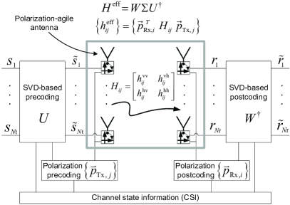
Figure 1: PR-MIMO system with polarization reconfigurable antennas.

III Polarization Pre-post Coding at the Polarization reconfigurable Antenna

III-A Polarization Precoding and Postcoding with Optimal Tx- and Rx-polarization

The Tx and the Rx can utilize SVD-based precoding and postcoding under the assumption of full CSIT and CSIR. The combination of SVD-based precoding and postcoding achieves the MIMO channel capacity for a given channel matrix via constructing parallel channels [37]. On the other hand, the MIMO communication system with polarization reconfigurable antennas in Fig. 1 can tune of the effective channel impulse response matrix $H^{\rm eff}$ itself in (1) by either polarization precoding at the Tx or polarization postcoding at the Rx; or joint polarization pre-post coding at both ends. We first focus on polarization precoding in this section.

The effective channel impulse response matrix can be decomposed by SVD as

$$H^{\rm eff}=W\Sigma U^{{\dagger}},$$ (5)

where $\Sigma$ is a diagonal matrix containing singular values, and $W$ and $U^{{\dagger}}$ are unitary matrices composed of the left and right singular vectors, respectively [37]. In this paper, $(\cdot)^{\dagger}$ is the Hermitian transpose operation. The channel capacity with SVD-based precoding and postcoding is

$$C=\sum_{k=1}^{R_{H^{\rm eff}}}\log_{2}\left(1+\frac{P_{k}}{{\sigma_{n}}^{2}}{\sigma_{k}}^{2}\right),$$ (6)

where $R_{H^{\rm eff}}$ is the rank of the matrix $H^{\rm eff}$, and $P_{k}$ is the power allocated to the $k$th eigenmode. Further, $\sigma_{k}$ is the $k$th singular value of the effective channel impulse response matrix $H^{\rm eff}$, and ${\sigma_{n}}^{2}$ is the noise power. Capacity maximization is achieved by a power allocation $P_{k}$ that satisfies waterfilling conditions

$$P_{k}=\max\left(0,\epsilon-\frac{{\sigma_{n}}^{2}}{{\sigma_{k}}^{2}}\right){\rm~{}s.t.~{}}P=\sum_{k=1}^{R_{H^{\rm eff}}}P_{k}{~{}},$$ (7)

i.e., the threshold $\epsilon$ is determined by the constraint of the total transmitted power P. We assume the total power is independent of the number of antennas.

Following [38], we use Jensen’s inequality to obtain

$$C \leq R_{H^{\rm eff}}{~{}}\log_{2}\left(1+\frac{1}{R_{H^{\rm eff}}}\sum_{k=1}^{R_{H^{\rm eff}}}\frac{P_{k}}{{\sigma_{n}}^{2}}{\sigma_{k}}^{2}\right)$$ (8)

$$= R_{H^{\rm eff}}{~{}}\log_{2}\left(\frac{1}{R_{H^{\rm eff}}}\frac{\epsilon}{{\sigma_{n}}^{2}}\sum_{k=1}^{R_{H^{\rm eff}}}{\sigma_{k}}^{2}\right),$$ (9)

where high SNR is assumed; all $P_{k}$ is greater than zero, i.e., $P_{k}=\epsilon-{\sigma_{n}}^{2}/{\sigma_{k}}^{2}>0$ in (7). Further, ${\sigma_{k}}^{2}$ is the eigenvalue of $\left(H^{\rm eff}(H^{\rm eff})^{\dagger}\right)$; therefore [39],

$$\sum_{k=1}^{R_{H^{\rm eff}}}{\sigma_{k}}^{2} = {\rm Tr}\left(H^{\rm eff}(H^{\rm eff})^{\dagger}\right)=\sum_{n,m}\left|h_{nm}^{\rm eff}\right|^{2}.$$ (10)

This is the sum of squared envelopes of all channel impulse response elements in $H^{\rm eff}$. This quantity is not only important for the channel capacity, but will also play an important role in the performance assessment of PR-HS/MRT systems, since the bounds employed there make use of it.

It is worth emphasizing that each element of $H^{\rm eff}$ is affected by the Tx- and Rx-polarization as implied in (1). Hence, the polarization vectors at polarization reconfigurable antenna elements impact constructively or destructively the MIMO channel capacity itself, even though SVD-based precoding/postcoding reaches the MIMO channel capacity for the given full CSIR/CSIT. The $j$th Tx polarization-agile antenna affects the $j$th column in (1); thus, the sum of squared singular values in (10) can be written as

$$\sum_{k=1}^{R_{H^{\rm eff}}}{\sigma_{k}}^{2} = \sum_{j=1}^{N_{\rm t}}\sum_{i=1}^{N_{\rm r}}\vec{p}_{{\rm Tx},j}^{~{}T}\left(H_{ij}^{{\dagger}}\vec{p}_{{\rm Rx},i}\vec{p}_{{\rm Rx},i}^{~{}T}H_{ij}\right)\vec{p}_{{\rm Tx},j}$$ (11)

$$= \sum_{j=1}^{N_{\rm t}}\vec{p}_{{\rm Tx},j}^{~{}T}H_{{\rm Tx},j}^{\rm PD}\vec{p}_{{\rm Tx},j}{~{}},$$

where the “Tx-polarization-determinant matrix” for the $j$th Tx polarization-agile antenna, $H_{{\rm Tx},j}^{\rm PD}$, is defined as

$$H_{{\rm Tx},j}^{\rm PD} \triangleq \sum_{i=1}^{N_{\rm r}}H_{ij}^{\dagger}\vec{p}_{{\rm Rx},i}\vec{p}_{{\rm Rx},i}^{~{}T}H_{ij}{~{}}.$$ (12)

The Tx-polarization vector at each Tx polarization-agile antenna is independent of those at other Tx-polarization antennas; therefore, the optimal Tx-polarization vector at the $j$th Tx polarization-agile antenna, $\vec{p}_{{\rm Tx},j}$, is the one which maximizes $\vec{p}_{{\rm Tx},j}^{~{}T}H_{{\rm Tx},j}^{\rm PD}\vec{p}_{{\rm Tx},j}$ in (11).

From the viewpoint of the linear-algebraic approach, $\vec{p}_{{\rm Tx},j}^{~{}T}H_{{\rm Tx},j}^{\rm PD}\vec{p}_{{\rm Tx},j}$ is positive semi-definite; thus, the equation, $\vec{p}_{{\rm Tx},j}^{~{}T}{~{}}H_{{\rm Tx},j}^{\rm PD}{~{}}\vec{p}_{{\rm Tx},j}=c_{j}$ corresponds to the ellipse as portrayed in Fig. 2, where $x$ and $y$ coordinates correspond to the elements of $\vec{p}_{{\rm Tx},j}$, i.e., $p_{{\rm Tx},j}^{\rm v}$ and $p_{{\rm Tx},j}^{\rm h}$, respectively [39]. Geometrically, the principal axes of the ellipse are along eigenvectors of the matrix $H_{{\rm Tx},j}^{\rm PD}$, $\overrightarrow{e}_{1}$ and $\overrightarrow{e}_{2}$, and the distances from the origin to the ellipse along the principal axes are $c_{j}/\sqrt{\lambda_{1}^{\rm PD}}$ and $c_{j}/\sqrt{\lambda_{2}^{\rm PD}}$, where $\lambda_{1}^{\rm PD}$ and $\lambda_{2}^{\rm PD}$ are the eigenvalues of $H_{{\rm Tx},j}^{\rm PD}$.

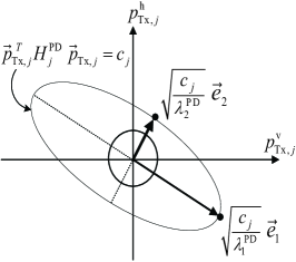
Figure 2: Polarization-determinant ellipse and polarization-vector unit circle.

Our objective at this stage is to estimate the optimal Tx-polarization vector at each Tx polarization-agile antenna element, $\vec{p}_{{\rm Tx},j}\in j=\{1,\cdots,N_{\rm t}\}$, which maximizes the column-sum of element-wise squared envelopes in $H^{\rm eff}$, i.e., $\vec{p}_{{\rm Tx},j}^{~{}T}H_{{\rm Tx},j}^{\rm PD}\vec{p}_{{\rm Tx},j}$. On the other hand, the Tx-polarization vector $\vec{p}_{{\rm Tx},j}$ is on the unit circle as presented in (3); therefore, the ellipse must have, at least, one intersection or contact point with the unit circle; whereas, at the same time it must make $\vec{p}_{{\rm Tx},j}^{~{}T}H_{{\rm Tx},j}^{\rm PD}\vec{p}_{{\rm Tx},j}=c_{j}$ as large as it can. Hence, the optimal Tx-polarization vector $\vec{p}_{{\rm Tx},j}^{\rm opt}$ and corresponding optimal Tx-polarization angle $\theta_{j}^{\rm opt}$ described in (3) are as

$$\vec{p}_{{\rm Tx},j}^{\rm~{}opt} = \arg\max\limits_{\vec{p}_{{\rm Tx},j}}{~{}}\vec{p}_{{\rm Tx},j}^{~{}T}H_{{\rm Tx},j}^{\rm PD}\vec{p}_{{\rm Tx},j}={~{}}\vec{e}_{2},$$ (13)

$$\theta_{j}^{\rm opt} = \arctan(\vec{e_{2}}).$$ (14)

Notice that $\vec{e}_{2}$ is the eigenvector corresponding to $\lambda_{2}$, which is the maximum eigenvalue of the Tx-polarization-determinant matrix, $H_{{\rm Tx},j}^{\rm PD}$. In this manner, each Tx polarization-agile antenna element can perform polarization precoding with the optimal Tx-polarization vector.

In a completely analogous manner, the optimal RX-polarization vector can be derived; we just now have to employ the row-sum (instead of the column-sum) of element-wise squared envelopes in $H^{\rm eff}$. The optimum polarization vector can be shown to be

$$\vec{p}_{{\rm Rx},i}^{\rm~{}opt} = \arg\max\limits_{\vec{p}_{{\rm Rx},i}}{~{}}\vec{p}_{{\rm Rx},i}^{~{}T}H_{{\rm Rx},i}^{\rm PD}\vec{p}_{{\rm Rx},i}={~{}}\vec{e}_{2},$$ (15)

$$\theta_{i}^{\rm opt} = \arctan(\vec{e_{2}}),$$ (16)

where the “Rx-polarization-determinant matrix” for the $i$th Rx polarization-agile antenna, $H_{{\rm Rx},i}^{\rm PD}$, is defined as

$$H_{{\rm Rx},i}^{\rm PD} \triangleq \sum_{j=1}^{N_{\rm t}}H_{ij}\vec{p}_{{\rm Tx},j}\vec{p}_{{\rm Tx},j}^{~{}T}H_{ij}^{\dagger}{~{}}.$$ (17)

III-B Joint Polarization Pre-post Coding for Polarization Matching

The Tx-polarization-determinant matrix at the $j$th Tx polarization-agile antenna, $H_{{\rm Tx},j}^{\rm PD}$, depends on the Rx-polarization vectors $\vec{p}_{{\rm Rx},i}$ as shown in (12), and vice versa in (17). Further, Tx- and Rx-polarization mismatching will deteriorate the system performance in terms of the channel capacity in this paper. For those reasons, joint polarization pre-post coding is required to maximize PR-MIMO channel capacity.

Joint optimization of the pre-post coding is difficult to obtain in closed form (and also difficult to implement); therefore, we propose an iterative approach where one iteration is a sequential loop of polarization precoding; then polarization postcoding. In the $q$th iteration stage, $\vec{p}^{{\rm~{}opt},(q)}_{{\rm Tx},j}$ is updated to $\vec{p}^{{\rm~{}opt},(q+1)}_{{\rm Tx},j}$ based on $\vec{p}^{{\rm~{}opt},(q)}_{{\rm Rx},i}$ according to (12) – (14). Then, in turn, $\vec{p}^{{\rm~{}opt},(q)}_{{\rm Rx},i}$ is updated to $\vec{p}^{{\rm~{}opt},(q+1)}_{{\rm Rx},i}$ based on the updated $\vec{p}^{{\rm~{}opt},(q)}_{{\rm Tx},j}$ following (15) – (17). If initial values of Rx and Tx polarization vectors are

$$\vec{p}_{{\rm Tx},j}^{\ (0)} = \begin{bmatrix}p_{{\rm Tx},j}^{\rm v}\\ p_{{\rm Tx},j}^{\rm h}\\ \end{bmatrix}=\begin{bmatrix}1\\ 0\\ \end{bmatrix},$$ (18)

$$\vec{p}_{{\rm Rx},i}^{\ (0)} = \begin{bmatrix}p_{{\rm Rx},i}^{\rm v}\\ p_{{\rm Rx},i}^{\rm h}\\ \end{bmatrix}=\begin{bmatrix}1\\ 0\\ \end{bmatrix},$$ (19)

the joint optimization iteration is expressed as

$$\vec{p}_{{\rm Tx},j}^{\rm~{}opt,(q+1)} = \arg\max\limits_{\vec{p}_{{\rm Tx},j}}{~{}}\vec{p}_{{\rm Tx},j}^{~{}T}H_{{\rm Tx},j}^{\rm PD,(q+1)}\vec{p}_{{\rm Tx},j}$$ (20)

$$H_{{\rm Tx},j}^{\rm PD,(q+1)} = \sum_{i=1}^{N_{\rm r}}H_{ij}^{\dagger}\vec{p}_{{\rm Rx},i}^{\rm~{}(q)}\vec{p}_{{\rm Rx},i}^{~{}T(q)}H_{ij}{~{}}.$$ (21)

$$\vec{p}_{{\rm Rx},i}^{\rm~{}opt,(q+1)} = \arg\max\limits_{\vec{p}_{{\rm Rx},i}}{~{}}\vec{p}_{{\rm Rx},i}^{~{}T}H_{{\rm Rx},i}^{\rm PD,(q+1)}\vec{p}_{{\rm Rx},i}$$ (22)

$$H_{{\rm Rx},i}^{\rm PD,(q+1)} = \sum_{j=1}^{N_{\rm t}}H_{ij}^{\dagger}\vec{p}_{{\rm Tx},j}^{\rm~{}(q)}\vec{p}_{{\rm Tx},j}^{~{}T(q)}H_{ij}{~{}},$$ (23)

$$h^{\rm eff}_{\rm opt,ij}=(\vec{p}_{{\rm Rx},i}^{\rm~{}opt,(q+1)})^{T}H_{ij}\vec{p}_{{\rm Tx},j}^{\rm~{}opt,(q+1)}~{},$$ (24)

where q is the iteration index. Note that while each step increases the capacity, the procedure is not guaranteed to reach the global optimum. However, we will see in Section VII that the capacity resulted from the iterative joint pre-post coding is in a close agreement with the one achieved by brute-force numerical search over all pre-post coding vectors.

IV Antenna Selection with Reconfigurable Polarization

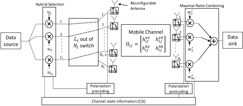
Figure 3: System Model of Antenna Selection with Reconfigurable Antennas

This section delineates the communication system that performs polarization reconfigurable hybrid selection (PR-HS) and MRT with the selected polarization reconfigurable Tx antenna elements as depicted in Fig. 3. The Tx selects $L_{t}$ out of $N_{t}$ polarization reconfigurable Tx antenna elements, and performs MRT with the associated weights $\{u_{1};u_{2},...,u_{L_{t}}\}$. At the same time, conventional MRC (without selection) is applied for multiple polarization reconfigurable antennas with corresponding weights $\{w^{*}_{1},w^{*}_{2},...,w^{*}_{N_{r}}\}$ at the Rx in Fig. 3. Each antenna element is polarization reconfigurable and adjusted to an optimal polarization angle based on the joint polarization pre-post coding proposed and described in Section III. In the same fashion as the PR-MIMO system, this section assumes perfect CSI. That is, both the Tx and Rx have perfect knowledge of the polarization-basis matrix in (1) – (2).

The partial channel impulse response matrix that represents the channels between selected polarization reconfigurable Tx antenna elements and Rx antenna elements is defined as $\widetilde{H}^{\rm eff}_{k}$, where the index $k$ stands for the $k$-th subset of $L_{t}$ number of antenna selection. Further, the column index matrix $C_{\rm Index}$ indicates the list of all possible combination of selected Tx antenna elements. That is,

$$C_{\rm Index}=\begin{bmatrix}\alpha_{11}&\ldots&\alpha_{1L_{t}}\\ &\vdots\\ \alpha_{\binom{N_{t}}{L_{t}}1}&\ldots&\alpha_{\binom{N_{t}}{L_{t}}L_{t}}\end{bmatrix},$$ (25)

where each row represents a subset of polarization reconfigurable Tx antenna indices corresponding to the selected antenna elements.

Each $\widetilde{H}^{\rm eff}_{k}$ consists of $L_{t}$ selected columns of $H^{\rm eff}$, associated with the selected polarization reconfigurable Tx antenna elements, and is described as

$$\widetilde{H}_{k}^{\rm eff}={{}{}{}{}{}{}{}{}{}{}{}{}{}{}{}{}{}{}{}{}{}{}{}{}{}{}{}{}{}{}{}{}{}{}{}{}{}{}{}{}{}{}{}{}{}{}{}{}{}{}{}{}{}{}{}{}{}{}}$$ (26)

$${}\begin{bmatrix}\vec{p}_{{\rm Rx},1}^{~{}T}H_{1\alpha_{k1}}\vec{p}_{{\rm Tx},\alpha_{k1}}&\ldots&\vec{p}_{{\rm Rx},1}^{~{}T}H_{1\alpha_{kL_{t}}}\vec{p}_{{\rm Tx},\alpha_{kL_{t}}}\\ \vdots&\ddots&\vdots\\ \vec{p}_{{\rm Rx},N_{\rm r}}^{~{}T}H_{N_{\rm r}\alpha_{k1}}\vec{p}_{{\rm Tx},\alpha_{k1}}&\ldots&\vec{p}_{{\rm Rx},N_{\rm r}}^{~{}T}H_{N_{\rm r}\alpha_{kL_{t}}}\vec{p}_{{\rm Tx},\alpha_{kL_{t}}}\end{bmatrix},{{}{}}$$

where $k$ corresponds to the $k$-th row of the column index matrix $C_{\rm Index}$. The achievable effective SNR of PR-HS/MRT is obtained based on SVD of $\widetilde{H}^{\rm eff}_{k}$ in (26) as

$$\gamma_{\rm PR-HS/MRT}^{\rm eff}=\underset{k}{\mathrm{max}}\big{(}{\widetilde{\sigma}_{k,\max}}^{~{}2}\big{)},$$ (27)

where $\widetilde{\sigma}_{k,\mathrm{max}}^{~{}2}$ is a maximum eigenvalue of $\widetilde{H}_{k}^{\rm eff}{\widetilde{H}_{k}^{{\rm eff}{\dagger}}}$ [29]. The objective is selecting the column index $k$ that maximize $\widetilde{\sigma}_{k,\mathrm{max}}^{~{}2}$. For further theoretical derivation,

$$\widetilde{H}_{k}^{\rm eff}\widetilde{H}_{k}^{\rm eff\dagger}=_{~{}~{}~{}~{}~{}~{}~{}~{}~{}~{}~{}~{}~{}~{}~{}~{}~{}~{}~{}~{}~{}~{}~{}~{}~{}~{}~{}~{}~{}~{}~{}~{}~{}~{}~{}~{}~{}~{}~{}~{}~{}~{}~{}~{}~{}~{}~{}~{}~{}~{}~{}~{}~{}~{}~{}}$$ (28)

$$\begin{bmatrix}&\vec{p}_{\rm Rx,1}^{~{}T}H^{\rm PD}_{\rm Rx,1}\vec{p}_{\rm Rx,1}&\ldots&\vec{p}_{\rm Rx,1}^{~{}T}H^{\rm Off}_{\rm Rx,1N_{r}}\vec{p}_{\rm Rx,N_{r}}\\ &\vdots&\ddots&\vdots\\ &\vec{p}_{\rm Rx,N_{r}}^{~{}T}H^{\rm Off}_{\rm Rx,N_{r}1},\vec{p}_{\rm Rx,1}&\ldots&\vec{p}_{\rm Rx,N_{r}}^{~{}T}H^{\rm PD}_{\rm Rx,N_{r}},\vec{p}_{\rm Rx,N_{r}}\end{bmatrix},$$

where

$$H^{\rm Off}_{{\rm Rx},ij}=\sum_{j=1}^{L_{\rm t}}H_{i\alpha_{ij}}\vec{p}_{{\rm Tx},\alpha_{ij}}\vec{p}_{{\rm Tx},\alpha_{ij}}^{{~{}}T}H_{j\alpha_{ij}}^{\dagger}$$ (29)

is the polarization determinant matrix of off-diagonal components. The algorithm to maximize the diagonal components of the matrix is described by (16). As will be described in Section VI, the algorithm described in Section III-B maximizes the lower bound of $\widetilde{\sigma}_{k,\mathrm{max}}^{~{}2}$, which significantly improve the achievable effective SNR in (27). We propose two schemes of PR-HS/MRT to efficiently achieve polarization reconfigurable antenna selection. One of the primary contributions of this paper is enhancing the effective SNR performance based on two proposed schemes in this section.

IV-A Scheme-1: Element-Wise Polarization Reconfiguration

Polarization pre-post coding in Section III is accomplished with $\widetilde{H}_{k}^{\rm eff}$ for each $k$ in the scheme of element-wise polarization reconfiguration. Based on the adjusted polarization for each $\widetilde{H}_{k}^{\rm eff}$, the best $k$ in terms of the greatest $\widetilde{\sigma}_{k,\mathrm{max}}^{~{}2}$, is selected as $L_{t}$ number of Tx antenna elements. We denominate Scheme-1 as element-wise (EW) polarization reconfiguration, since optimal polarization vectors of every $\widetilde{H}_{k}^{\rm eff}$ for $k=\big{\{}1,2,...,\binom{N_{t}}{L_{t}}\big{\}}$ is estimated. The EW Rx optimal polarization vectors are defined as

$$\vec{p}_{{\rm Rx},i}^{{~{}}\rm EW} = \underset{\vec{p}_{{\rm Rx},i}}{\arg\max}{~{}}\vec{p}_{{\rm Rx},i}^{{~{}}T}H^{\rm EW}_{{\rm Rx},i}\vec{p}_{{\rm Rx},i}{~{}},$$ (30)

$$H^{\rm EW}_{{\rm Rx},i} = \sum_{j=1}^{L_{\rm t}}H_{i\alpha_{ij}}\vec{p}_{{\rm Tx},\alpha_{ij}}\vec{p}_{{\rm Tx},\alpha_{ij}}^{{~{}}T}H_{i\alpha_{ij}}^{\dagger}{~{}},$$ (31)

where (31) is EW Rx-polarization-determinant matrix. In a similar manner, the optimal polarization vectors at the Tx are described as

$$\vec{p}_{{\rm Tx},\alpha_{ij}}^{{~{}}\rm EW} = \underset{\vec{p}_{{\rm Tx},\alpha_{ij}}}{\arg\max}{~{}}\vec{p}_{{\rm Tx},\alpha_{ij}}^{{~{}}T}H^{\rm EW}_{{\rm Tx},\alpha_{ij}}\vec{p}_{{\rm Tx},\alpha_{ij}},$$ (32)

$$H^{\rm EW}_{{\rm Tx},\alpha_{ij}} = \sum_{i=1}^{N_{\rm r}}H_{i\alpha_{ij}}^{\dagger}\vec{p}_{{\rm Rx},i}\vec{p}_{{\rm Rx},i}^{{~{}}T}H_{i\alpha_{ij}}$$ (33)

where (33) is EW Tx-polarization-determinant matrix. With (30) and (32), each $\widetilde{H}^{\rm eff}_{k}$ is tuned with corresponding EW Tx/Rx polarization vectors. That is,

$$\widetilde{H}^{\rm eff}_{{\rm EW},k}{}={}$$ (34)

$$\begin{bmatrix}(\vec{p}_{{\rm Rx},1}^{~{}\rm EW})^{T}H_{1\alpha_{k1}}\vec{p}_{{\rm Tx},\alpha_{k1}}^{~{}\rm EW}\ldots(\vec{p}_{{\rm Rx},1}^{~{}\rm EW})^{T}H_{1\alpha_{kL_{t}}}\vec{p}_{{\rm Tx},\alpha_{kL_{t}}}^{~{}\rm EW}\\ \vdots~{}~{}~{}~{}~{}~{}~{}~{}~{}~{}~{}~{}\ddots~{}~{}~{}~{}~{}~{}~{}~{}~{}~{}~{}~{}~{}~{}\vdots\\ (\vec{p}_{{\rm Rx},N_{\rm r}}^{~{}\rm EW})^{T}H_{N_{\rm r}\alpha_{k1}}\vec{p}_{{\rm Tx},\alpha_{k1}}^{~{}\rm EW}\ldots(\vec{p}_{{\rm Rx},N_{\rm r}}^{~{}\rm EW})^{T}H_{N_{\rm r}\alpha_{kL_{t}}}\vec{p}_{{\rm Tx},\alpha_{kL_{t}}}^{~{}\rm EW}\end{bmatrix}.$$

The effective SNR with EW polarization reconfiguration is

$$\gamma_{\rm PR-HS/MRT}^{\rm EW}=\underset{k}{\mathrm{max}}\big{(}\widetilde{\sigma}_{k,{\rm max}}^{\rm EW}\big{)}^{2},$$ (35)

where $\big{(}\widetilde{\sigma}_{k,{\rm max}}^{\rm EW}\big{)}^{2}$ is a maximum eigenvalue of $\widetilde{H}_{{\rm EW},k}^{\rm eff}\widetilde{H}_{{\rm EW},k}^{{\rm eff}{~{}}\dagger}$.

IV-B Scheme-2: Global Polarization Reconfiguration

This scheme determines the polarization pre-post coding in Section III with the full $N_{r}\times N_{t}$ channel impulse response matrix regardless of $L_{t}$, the number of Tx antenna elements to be selected. Based on the global effective channel impulse response matrix $H^{\rm eff}$ rather than any partial channel impulse response matrix $\widetilde{H}_{k}^{\rm eff}$, $L_{t}$ number of Tx antenna elements are selected to maximize the effective SNR caused by MRT. Thus, the optimal polarization vectors for both Rx and Tx are aligned with (13) – (16). We denominate Scheme-2 as Global polarization reconfiguration; for the consistency, the optimal Rx and Tx polarization vectors of Scheme-2 are, respectively, expressed as

$$\vec{p}_{{\rm Rx},i}^{\rm~{}G}=\vec{p}_{{\rm Rx},i}^{\rm~{}opt}{~{}},$$ (36)

$$\vec{p}_{{\rm Tx},j}^{\rm~{}G}=\vec{p}_{{\rm Tx},j}^{\rm~{}opt}{~{}}.$$ (37)

The partial channel impulse response matrix associated with the selected $L_{t}$ number of polarization reconfigurable Tx antenna elements, $\widetilde{H}^{\rm eff}_{{\rm G},k}$ can be described as

$${}\widetilde{H}^{\rm eff}_{{\rm G},k}{}={}$$ (38)

$${}\begin{bmatrix}{}(\vec{p}_{{\rm Rx},1}^{~{}\rm G})^{T}H_{1\alpha_{k1}}\vec{p}_{{\rm Tx},\alpha_{k1}}^{~{}\rm G}\ldots(\vec{p}_{{\rm Rx},1}^{\rm~{}G})^{T}H_{1\alpha_{kL_{t}}}\vec{p}_{{\rm Tx},\alpha_{kL_{t}}}^{~{}\rm G}\\ \vdots~{}~{}~{}~{}~{}~{}~{}~{}~{}~{}~{}~{}\ddots~{}~{}~{}~{}~{}~{}~{}~{}~{}~{}~{}~{}~{}~{}\vdots\\ (\vec{p}_{{\rm Rx},N_{\rm r}}^{~{}\rm G})^{T}H_{N_{\rm r}\alpha_{k1}}\vec{p}_{{\rm Tx},\alpha_{k1}}^{~{}\rm G}\cdot\cdot(\vec{p}_{{\rm Rx},N_{\rm r}}^{\rm~{}G})^{T}H_{N_{\rm r}\alpha_{kL_{t}}}\vec{p}_{{\rm Tx},\alpha_{kL_{t}}}^{~{}\rm G}\end{bmatrix}.$$

The effective SNR in Scheme-2 is

$$\gamma_{\rm PR-HS/MRT}^{\rm G}=\underset{k}{\mathrm{max}}\big{(}\widetilde{\sigma}_{k,{\max}}^{\rm G}\big{)}^{2},$$ (39)

where $\big{(}\widetilde{\sigma}_{k,{\rm max}}^{\rm G}\big{)}^{2}$ is a maximum eigenvalue of $\widetilde{H}_{{\rm G},k}^{\rm eff}\widetilde{H}_{{\rm G},k}^{{\rm eff}{~{}}\dagger}$.

IV-C Comparison of Two Schemes

The effective SNR’s provided by PR-HS/MRT in Scheme-1 and Scheme-2 are proportional to $\big{(}\widetilde{\sigma}_{k,{\rm max}}^{\rm EW}\big{)}^{2}$ and $\big{(}\widetilde{\sigma}_{k,{\rm max}}^{\rm G}\big{)}^{2}$, respectively, for the given $k$, i.e., for the same set of $L_{t}$ Tx antenna elements.

$\big{(}\widetilde{\sigma}_{k,{\rm max}}^{\rm EW}\big{)}^{2}$ is a maximum eigenvalue of $\widetilde{H}_{{\rm EW},k}^{\rm eff}\widetilde{H}_{{\rm EW},k}^{{\rm eff}{~{}}\dagger}$, which is described as

$${}\widetilde{H}_{{\rm EW},k}^{\rm eff}\widetilde{H}_{{\rm EW},k}^{{\rm eff}{~{}}\dagger}{}={}$$ (40)

$${}\begin{bmatrix}(\vec{p}_{\rm Rx,1}^{\rm~{}EW})^{T}H^{\rm EW}_{\rm Rx,1}\vec{p}_{\rm Rx,1}^{\rm~{}EW}~{}~{}~{}~{}\ldots~{}~{}(\vec{p}_{\rm Rx,1}^{\rm~{}EW})^{T}H^{\rm Off}_{\rm Rx,1N_{r}}\vec{p}_{\rm Rx,N_{r}}^{\rm~{}EW}\\ \vdots~{}~{}~{}~{}~{}~{}~{}~{}~{}~{}~{}~{}~{}\ddots~{}~{}~{}~{}~{}~{}~{}~{}~{}~{}~{}~{}~{}~{}\vdots\\ (\vec{p}_{\rm Rx,N_{r}}^{\rm~{}EW})^{T}H^{\rm Off}_{\rm Rx,N_{r}1},\vec{p}_{\rm Rx,1}^{\rm~{}EW}\ldots(\vec{p}_{\rm Rx,N_{r}}^{\rm~{}EW})^{T}H^{\rm EW}_{\rm Rx,N_{r}},\vec{p}_{\rm Rx,N_{r}}^{\rm~{}EW}\end{bmatrix}$$

On the other hand, $\big{(}\widetilde{\sigma}_{k,{\rm max}}^{\rm G}\big{)}^{2}$ is a maximum eigenvalue of $\widetilde{H}_{{\rm G},k}^{\rm eff}\widetilde{H}_{{\rm G},k}^{{\rm eff}{~{}}\dagger}$ that is expressed as

$$\widetilde{H}_{{\rm G},k}^{\rm eff}\widetilde{H}_{{\rm G},k}^{{\rm eff}{~{}}\dagger}{}={}$$ (41)

$$\begin{bmatrix}(\vec{p}_{\rm Rx,1}^{\rm~{}G})^{T}H^{\rm G}_{\rm Rx,1}\vec{p}_{\rm Rx,1}^{\rm~{}G}~{}~{}~{}\ldots~{}~{}(\vec{p}_{\rm Rx,1}^{\rm~{}G})^{T}H^{\rm Off}_{\rm Rx,1N_{r}}\vec{p}_{\rm Rx,N_{r}}^{\rm~{}G}\\ \vdots~{}~{}~{}~{}~{}~{}~{}~{}~{}~{}~{}~{}\ddots~{}~{}~{}~{}~{}~{}~{}~{}~{}~{}~{}~{}~{}~{}\vdots\\ (\vec{p}_{\rm Rx,N_{r}}^{\rm~{}G})^{T}H^{\rm Off}_{\rm Rx,N_{r}1},\vec{p}_{\rm Rx,1}^{\rm~{}G}\ldots(\vec{p}_{\rm Rx,N_{r}}^{\rm~{}G})^{T}H^{\rm G}_{\rm Rx,N_{r}},\vec{p}_{\rm Rx,N_{r}}^{\rm~{}G}\end{bmatrix},$$

where the global Rx-polarization-determinant matrix, $H^{\rm G}_{\rm Rx,i}$ is

$$H^{\rm G}_{\rm Rx,i}=\sum_{j=1}^{L_{\rm t}}H_{i\alpha_{ij}}\vec{p}_{{\rm Tx},\alpha_{ij}}\vec{p}_{{\rm Tx},\alpha_{ij}}^{{~{}}T}H_{i\alpha_{ij}}^{\dagger}{~{}}.$$ (42)

The diagonal components of (40) are maximized with EW polarization reconfiguration, since each $\widetilde{H}^{\rm eff}_{{\rm EW},k}$ is tuned according to its optimal polarization vectors, as described in (30) – (33). Hence, effective SNR in (35) is maximized. Meanwhile, polarization vectors in global polarization reconfiguration are optimized for the full channel impulse response matrix; therefore, diagonal components of (41) are not maximized for $L_{t}<N_{t}$. That is, those diagonal elements are aligned with (13) – (16), which maximizes diagonal elements of $H^{\rm eff}(H^{\rm eff})^{\dagger}$. Nonetheless, global polarization reconfiguration also satisfactorily increases the effective SNR of the system even when applied to each $\widetilde{H}^{\rm eff}_{{\rm G},k}$. Further, as $L_{t}$ approaches $N_{t}$, $\widetilde{H}_{{\rm EW},k}^{\rm eff}$ approaches $\widetilde{H}_{{\rm G},k}^{\rm eff}$. Although EW polarization reconfiguration outperforms global polarization reconfiguration, the latter offers an advantage in the complexity and the corresponding computation time.

V Effect of polarization on the channel

V-A Random Polarization Vectors

One of the primary contributions of this paper is the statistical analysis of the polarization reconfigurable wireless channels for the scenarios of PR-MIMO and PR-HS/MRT. This section analyzes the impact of deploying polarization reconfigurable antenna elements on the conventional MIMO system. Random polarization is first considered; then, the impact of the proposed polarization pre-post coding on the MIMO channel is scrutinized. The elements of polarization-basis matrix, described in (2), are modeled as independent and identically distributed (i.i.d.) complex Gaussian random variables with zero mean and unit variance. Each element of $H^{\rm eff}$ can be expressed as

$$h_{ij}^{\rm eff} = \vec{p}^{~{}T}_{{\rm Rx},i}\begin{bmatrix}h^{\rm vv}_{ij}&h^{\rm vh}_{ij}\\ h^{\rm hv}_{ij}&h^{\rm hh}_{ij}\end{bmatrix}\vec{p}_{{\rm Tx},j}~{}~{}~{}~{}~{}~{}~{}~{}~{}~{}~{}~{}~{}~{}~{}~{}~{}~{}~{}~{}$$ (43)

$$= h^{\rm vv}_{ij}\cos(\theta_{j})\cos(\theta_{i})+h^{\rm hv}_{ij}\sin(\theta_{i})\cos(\theta_{j})$$

$$+h^{\rm vh}_{ij}\cos(\theta_{i})\sin(\theta_{j})+h^{\rm hh}_{ij}\sin(\theta_{j})\sin(\theta_{i}).$$

$$= \beta_{1}+\beta_{2}+\beta_{3}+\beta_{4}~{}.$$

For convenience, we abbreviate the four terms in (43) as $\beta_{1}$, $\beta_{2}$, $\beta_{3}$ and $\beta_{4}$, respectively, in the order of the expression in (43). Considering the random movement and rotation of the UE along with depolarization of the wireless channel itself [20, 25], the probability density function (pdf) of the polarization angles, $f_{\Theta}(\theta)$ can be expressed as

$$f_{\Theta}(\theta)=\left\{\begin{array}[]{ll}\frac{1}{2\pi}~{},&\quad\rm if\ \theta\ \in\left[-\pi,\pi\right].\\ \\ 0~{},&\quad\rm otherwise.\end{array}\right.$$ (47)

The random variable, $\Theta\sim U(-\pi,\pi)$, can be transformed to $Y=\cos(\Theta)$ and $X=\sin(\Theta)$, where we are interested in the pdf’s of $Y$ and $X$. The cumulative distribution functions (cdf’s) of $\Theta$ and $Y=\cos(\Theta)$, i.e., $F_{\Theta}$ and $F_{Y}$, respectively, are as

$$F_{\Theta}(\theta)=\dfrac{\theta}{\pi}{~{}},{~{}~{}~{}}F_{Y}(y)=\dfrac{\arccos(y)}{\pi}{~{}}.$$ (48)

Based on (48) the pdf of $Y$, $f_{Y}$ is derived; in the similar fashion, the pdf of $X=\sin(\Theta)$, $f_{X}$ is obtained as

$$f_{Y}(y)=\dfrac{1}{\pi}\dfrac{1}{\sqrt{1-y^{2}}},{~{}~{}~{}}f_{X}(x)=\dfrac{1}{\pi}\dfrac{1}{\sqrt{1-x^{2}}}{~{}}.$$ (49)

The distributions of $Y=\cos(\Theta)$ and $X=\sin(\Theta)$ are portrayed in Fig. 4, where $\Theta$ is independently generated $10^{6}$ times. The curve fitting of the empirical distribution exhibits excellent agreement with the theoretical analysis in (49).

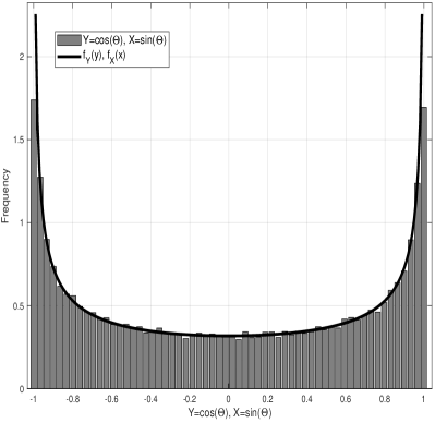
Figure 4: Distribution of the elements in polarization vector: $Y=\cos(\Theta)$ and $X=\sin(\Theta)$

.

The mean and variance of (49) and (49) are 0 and 1/2, respectively; furthermore, the variance of $h^{\rm eff}$ is

$${\rm Var}(h^{\rm eff}_{ij})={\rm Var}(\beta_{1})+{\rm Var}(\beta_{2})+{\rm Var}(\beta_{3})+{\rm Var}(\beta_{4}).$$ (50)

Owing to the page limit, the extensive description of deriving expectation and variance of (49) as well as (50) is provided in Appendix A. Three terms in each $\beta_{i}$ for $i\in\{1,2,3,4\}$ are independent of each other. Thus, the variance of the real and imaginary parts in $\beta_{i}$ is $\frac{1}{2}\times\frac{1}{2}\times\frac{1}{2}=\frac{1}{8}$; consequently, $h^{\rm eff}_{ij}$ has unit variance as described in detail in Appendix A. It is noteworthy that the mean and variance of reconfigurable antennas with random channel polarization are the same as those of conventional channels without polarization reconfigurable antenna elements. Furthermore, the squared envelope of $h^{\rm eff}_{ij}$, with random polarization, follows chi-square distribution with 2 degrees of freedom.

V-B Optimal Polarization Vectors

It is worth emphasizing that combination of antenna selection and polarization reconfiguration, i.e., PR-HS can provide significant improvement in channel gain, i.e., the squared envelop of $h^{\rm eff}_{ij}$. The proposed polarization pre-post coding scheme is based on the closed-form derivation for the optimal polarization vectors at one end; whereas, the globally optimal polarization vectors at both ends of the Tx and Rx are achieved by the iterative methodology. Hence, the complete analysis to reach the closed-form description is unfeasible. However, the comprehensive simulation results in Fig. 5 show that the proposed PR-HS scheme improves the system performance in terms of SNR and the associated distribution of channel gain.

Empirical distributions of channel gain, i.e., $h^{\rm eff}_{ij}$ are depicted in Fig. 5, where the PR-MIMO system applied PR-HS antenna selection with $N_{t}=8$ and $L_{t}\in\{1,2,...,8\}$. In each channel realization, the average of $h^{\rm eff}_{ij}$ exhibits significantly improved distribution in terms of mean, variance and the overall tendency of the distributions.

As $L_{t}$ increases to reach $N_{t}=8$, the empirical distribution converge to chi-square distribution with 4 degrees of freedom, which is the normal case with conventional system without proposed schemes and algorithms in this paper. The scenario that $L_{t}=3$ still has substantial benefit of PR-HS scheme. The distribution is not chi-square distributed, since the selection process leads to ordered statistics. However, we can observe empirically that the resulting distribution has a mean similar to that of a chi-square distribution with 8 degrees of freedom; however, lower/better variance. In the scenario that $L_{t}=1$, the mean of the empirical distribution is similar to that of chi-square distribution with 12 degrees of freedom. In contrast, the variance of the empirical distribution is lower than chi-square distribution with 12 degrees of freedom, which will be helpful for the gNB to accomplish stable link adaptation including adaptive modulation and coding.

Without loss of generality, an element in $H^{\rm eff}$ has the following description of its squared envelop.

$$|h^{\rm eff}_{11}|^{2}=\vec{p}_{{\rm Rx},1}^{~{}T}\big{(}H_{11}\vec{p}_{{\rm Tx},1}\vec{p}_{{\rm Tx},1}^{~{}T}H_{11}^{\dagger}\big{)}\vec{p}_{{\rm Rx},1}~{}.$$ (51)

From the Analysis of (51), we can have an intuition for the mathematical interpretation of the aforementioned simulation results. However, owing to the page limit, Appendix B provides further analysis on (51).

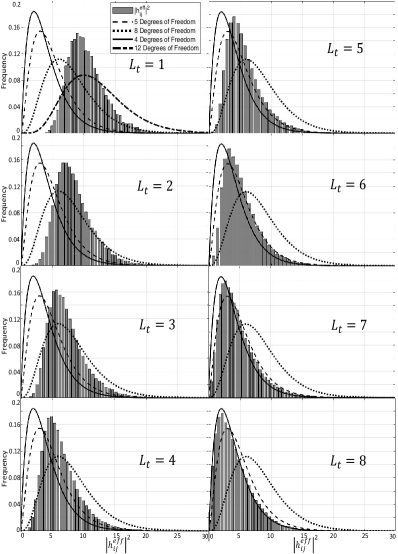
Figure 5: Empirical distribution of $|h^{\rm eff}_{ij}|^{2}$ in PR-HS; the comparison of chi-square distribution with 4, 5, 8, 12 degrees of freedom.

VI Statistics of Achievable SNR in PR-HS/MRT

VI-A Upper and Lower Bounds

The analytical solution of (27) cannot be easily obtained; however, for the $k$-th set of $L_{t}$ Tx antenna elements, the closed form analysis of upper and lower bounds of the effective SNR can be described as

$$\dfrac{1}{{\rm min}(L_{t},N_{r})}\sum_{m}\big{(}\widetilde{\sigma}^{\rm EW}_{k,m}\big{)}^{2}\leq\big{(}\widetilde{\sigma}^{\rm EW}_{k,{\rm max}}\big{)}^{2}\leq\sum_{m}\big{(}\widetilde{\sigma}^{\rm EW}_{k,m}\big{)}^{2},$$ (52)

i.e., the achievable SNR for a polarization reconfigurable channel matrix is lower bounded by the average of the nonzero eigenvalues of $\widetilde{H}_{{\rm EW},k}^{\rm eff}\widetilde{H}_{{\rm EW},k}^{{\rm eff}{~{}}\dagger}$ and upper bounded by the sum of the nonzero eigenvalues of $\widetilde{H}_{{\rm EW},k}^{\rm eff}\widetilde{H}_{{\rm EW},k}^{{\rm eff}{~{}}\dagger}$. We take into account EW polarization reconfiguration (Scheme-1), since it outperforms global polarization reconfiguration (Scheme-2). The upper bound of achievable SNR in PR-HS scheme is

$$\gamma_{\rm UpperBound} = \underset{k}{\mathrm{max}}\bigg{(}\sum_{m}\big{(}\widetilde{\sigma}^{\rm EW}_{k,m}\big{)}^{2}\bigg{)}$$

$$= \underset{k}{\mathrm{max}}\bigg{(}\sum_{i}\sum_{j}|\widetilde{h}^{\rm eff}_{{\rm EW},k,ij}|^{2}\bigg{)}.$$

In a similar manner, the lower bound is described as,

$$\gamma_{\rm LowerBound} = \dfrac{1}{\min(L_{t},N_{r})}\underset{k}{\mathrm{max}}\bigg{(}\sum_{m}\big{(}\widetilde{\sigma}^{\rm EW}_{k,m}\big{)}^{2}\bigg{)}$$

$$= \dfrac{\underset{k}{\mathrm{max}}\bigg{(}\sum_{i}\sum_{j}|\widetilde{h}^{\rm eff}_{{\rm EW},k,ij}|^{2}\bigg{)}}{\min(L_{t},N_{r})}~{},$$

The joint statistics of the ordered SNRs can be described as

$$\rho_{\gamma(j)}(\gamma_{(1)},\gamma_{(2)},...,\gamma_{(N_{t})}){}{}{}{}{}{}{}{}{}{}{}{}{}{}{}{}{}{}{}{}{}{}{}{}{}{}{}{}{}{}{}{}{}{}{}{}{}{}{}$$ (55)

$$=\left\{\begin{array}[]{ll}N_{t}!\prod\limits_{i=1}^{N_{t}}\dfrac{1}{\Gamma(N_{r})}\gamma_{(j)}^{\rm N_{r}-1}\\ \times{\rm exp}\big{(}-\gamma_{(j)}\big{)},&{\rm for}~{}\gamma_{(1)}<\gamma_{(2)}<...\gamma_{(N_{t})}\\ \\ 0,&\rm otherwise\end{array}\right.$$

where $\Gamma(.)$ is the Euler Gamma Function [29]. We utilize $L_{t}$ out of $N_{t}$ variables $\gamma_{(i)}$; choose the $k$-th row of the column index matrix $C_{\rm Index}$ in (25) that provides maximum achievable SNR in PR-HS/MRT. The desired $\gamma_{\rm UpperBound}$ can be written in terms of the ordered SNRs as

$$\gamma_{\rm UpperBound}=\sum_{i=1}^{L_{t}}\gamma_{(j)}.$$ (56)

$\gamma_{\rm UpperBound}$ in (56) is the sum of random variables; the corresponding characteristic function is useful for further analysis. It is described as [29]

$$\Phi(j\nu){}={}$$ (57)

$${~{}~{}~{}~{}~{}~{}}\dfrac{N_{t}!}{[\Gamma(N_{r})]^{N_{t}}}\int_{0}^{\infty}d\gamma_{(1)}\gamma_{(1)}^{N_{r}-1}e^{-\gamma_{(1)}}e^{-j\nu\Xi(L_{t}-1)\gamma_{(1)}}$$

$${~{}~{}~{}~{}~{}~{}}\times\int_{0}^{\gamma_{(1)}}d\gamma_{(2)}\gamma_{(2)}^{N_{r}-1}e^{-\gamma_{(2)}}e^{-j\nu\Xi(L_{t}-1)\gamma_{(2)}}...~{}~{}~{}~{}~{}~{}~{}~{}~{}$$

$${~{}~{}~{}~{}~{}~{}}\times\int_{0}^{\gamma_{(N_{t}-1)}}d\gamma_{(N_{t})}\gamma_{(N_{t})}^{N_{r}-1}e^{-\gamma_{(N_{t})}}e^{-j\nu\Xi(L_{t}-1)\gamma_{(N_{t})}},~{}$$

where $\Xi(x)$ is the Heaviside step function

$$\Xi(x)=\left\{\begin{array}[]{ll}1,&\quad\rm if\ x\leq 0,\\ \\ 0,&\quad\rm otherwise.\end{array}\right.$$ (61)

In the following, we abbreviate the expression $1+j\nu\Xi(L_{t}-i)$ as $a_{i}$, dropping the dependence on $\nu$ for notational convenience. The rest of derivation is refered from [29].

The characteristic function of $\gamma_{\rm UpperBound}$ is finally provided as

$$\Phi(j\nu) =\dfrac{N_{t}!}{[\Gamma(N_{r})]^{N_{t}}}\bigg{[}d^{N_{t}-1}(N_{r}-1)!a_{1}^{-N_{r}}$$ (62)

$$+\sum_{\rho=1}^{N_{t}-1}\sum_{t=0}^{(N_{t}-\rho+1)(N_{r}-1)}\hat{c}_{\rho,t}^{(N_{t}-1)}t!(b_{p}^{N_{t}})^{-(t+1)}\bigg{]}.$$

VI-B Channel Capacity and Symbol Error Rate

The instantaneous channel capacity for each channel realization is given by

$$C(\gamma_{\rm PR-HS/MRT}^{\rm x})=\rm log_{2}\big{[}1+\bar{\Gamma}(\gamma_{\rm PR-HS/MRT}^{\rm x})\big{]},$$ (63)

where ${\rm x}\in\{\rm EW,G\}$ and $\bar{\Gamma}$ is the average SNR of a single-input single-output (SISO) channel. Lower and upper bounds of the system can be applied to this equation by substituting $\gamma_{\rm LowerBound}$ and $\gamma_{\rm UpperBound}$ for $\gamma_{\rm PR-HS/MRT}$ in (63). In the case of quadrature phase shift keying (QPSK) modulation, the instantaneous SER is

$$SER_{n}=1-\bigg{[}1-Q\bigg{(}\sqrt{\bar{\Gamma}(\gamma_{\rm PR-HS/MRT}^{\rm x})_{n}}\bigg{)}\bigg{]}^{2},$$ (64)

where $n=1,2,....N$ and $N$ is total number of channel realizations. Finally, average SER is represented as

$$\overline{SER}=\dfrac{1}{N}\sum_{n=1}^{N}SER_{n}~{}.$$ (65)

VII Numerical Experiments and Results

VII-A Simulations in PR-MIMO

In this section we provide evaluations of our closed-form equations for optimum polarization vectors and the associated PR-MIMO channel capacity. We also compare the results to brute-force numerical optimization, where we step through all possible (discretized) values of the Tx/Rx-polarization angle and choose the optimal values that correspond to the maximum capacity for each PR-MIMO channel realization. The step width of the brute-force numerical search are, respectively, $1^{\circ}$ in Figs. 6 and 7; $5^{\circ}$ in Figs. 8 and 9; $10^{\circ}$ in Figs. 10 and 11. Unless stated otherwise, we consider independent and identically distributed (i.i.d.) Rayleigh fading channels with a cross-polarization discrimination, ${\rm XPD}=0{\rm~{}dB}$.

We first investigate the impact of polarization reconfiguration in several deterministic channels. The PR-MIMO channel capacity in a $2\times 2$ system with polarization reconfigurable antenna elements is shown for varying Tx-polarization angles in Figs. 6 and 7. The relatively low SNR regime such as 5 dB and the very high SNR regime such as 30 dB are shown in Figs. 6 and 7, respectively. In both scenarios, the channel capacity obtained by the polarization precoding at the Tx exhibits negligible difference from that yielded by the numerical result as indicated in both figures. For the 5 dB SNR in Fig. 6, the theoretically derived optimal Tx-polarization angles themselves have insignificant differences from numerically derived optimal Tx-polarization angles. In contrast, in the very high SNR regime in Fig. 7, the differences between theoretically and numerically obtained optimal Tx-polarization angles are considerable. This is due to the fact that the approximation (8) is less accurate at higher SNRs. However, the difference in capacity is still remarkably small. In case of polarization postcoding at the Rx, similar results are attained owing to the symmetry described in Sections III-A; therefore, the results are omitted here. It is worth mentioning that optimal Tx- or Rx-polarization vectors are not necessarily orthogonal, which corresponds to $90^{\circ}$ difference in Tx- or Rx-polarization angles, as described in Figs. 6 and 7.

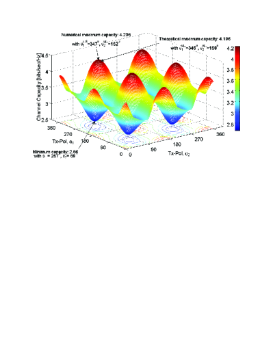
Figure 6: Channel capacity for varying Tx-polarization; 5 dB SNR.

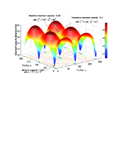
Figure 7: Channel capacity for varying Tx-polarization; 30 dB SNR.

The PR-MIMO channel capacity with the optimal Tx-polarization angles is demonstrated to depend on varying Rx-polarization angles in Fig. 8, where we also consider the $2\times 2$ RP-MIMO system with polarization-agile antenna elements at both ends of the Tx and the Rx. The channel capacity exhibits substantial variation from 21.47 bits/sec/Hz to 13.60 bits/sec/Hz depending on Rx-polarization angles, although Tx-polarization angles are already set to the optimum obtained by brute-force numerical search as will be shown in Fig. 9, i.e., $\theta_{{\rm Tx}-1}=80^{\circ}$; $\theta_{{\rm Tx}-2}=50^{\circ}$. This result obviously shows that the polarization mismatching between the Tx and the Rx can cause significant deterioration in the capacity of the whole system, even if one end of the Tx and the Rx is already set to the optimal polarization. However, the proposed scheme of joint polarization pre-post coding also shows negligible difference from numerical results in both optimal Tx- and Rx-polarization angles and channel capacity.

Local optimal Tx- and Rx-polarization vectors at each iteration of joint polarization pre-post coding are depicted in Fig. 9 considering the same scenario of channel impulse matrices and SNR as that in Fig. 8. The $2\times 2$ PR-MIMO system is again considered in this figure. Here, one iteration is a sequential loop of polarization precoding and then polarization postcoding as described in Section III-B. Tx/Rx-polarization vectors quickly converge; moreover, these global optimal polarization vectors show relatively small difference from the numerical optimum.

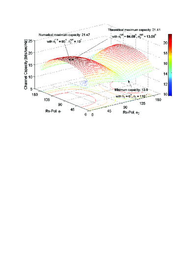
Figure 8: Channel capacity for varying Rx-polarization with optimal Tx-polarization; 30 dB SNR.

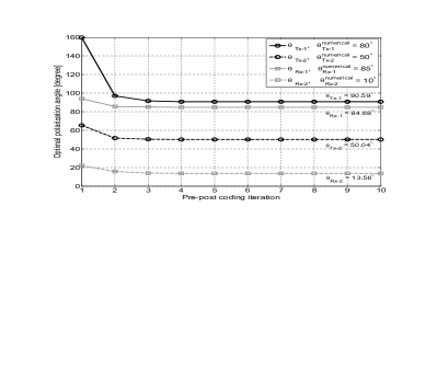
Figure 9: Optimal Tx/Rx-polarization angles for the number of iterations; 30 dB.

In contrast to Figs. 6 – 9, from this point on, we investigate how much the joint polarization pre-post coding improves the PR-MIMO channel capacity in a statistical sense in Figs. 10 – 12. The simulation results are based on the $10^{4}$ times realizations of i.i.d. Rayleigh fading channels. Figures 10 and 11 depict cumulative density functions (cdf’s) of the $2\times 2$ PR-MIMO channel capacity at 5 dB SNR and 30 dB SNR, respectively, for the scenarios of joint polarization pre-post coding with Tx/Rx polarization-agile antennas; and random Tx/Rx-polarization. It is noteworthy that the cdf resulting from the fixed Tx/Rx-polarization exhibits exactly the same cdf of random Tx/Rx-polarization at each channel realization owing to the random generation of the i.i.d. Rayleigh fading channels. Furthermore, the cdf’s of the optimal and the worst Tx/Rx-polarization obtained by brute-force numerical search at each channel realization, are presented in Figs. 10 and 11. We perform five iterations for the joint polarization pre-post coding at each PR-MIMO channel realization, which results in the satisfactory convergence of Tx/Rx-polarization vectors on the global optimal ones as demonstrated in Fig. 9.

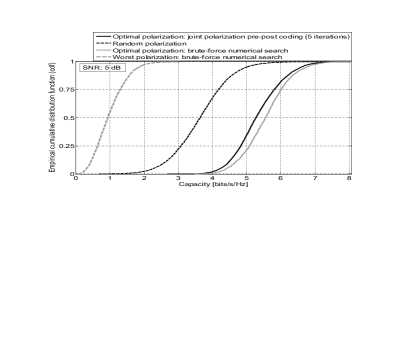
Figure 10: cdf’s of channel capacity for the scenarios of joint polarization pre-post coding with five iterations, random Tx/Rx-polarization; optimal and the worst Tx/Rx-polarization through brute-force numerical search at 5 dB SNR.

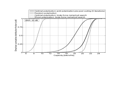
Figure 11: cdf’s of channel capacity for the scenarios of joint polarization pre-post coding with five iterations, random Tx/Rx-polarization; optimal and the worst Tx/Rx-polarization through brute-force numerical search at 30 dB SNR.

Our joint polarization pre-post coding significantly improves the PR-MIMO channel capacity at both 5 dB SNR and 30 dB SNR. In Fig. 10, the probability of the PR-MIMO channel capacity less than 4.2 bits/sec/Hz is 0.75 with 5 dB SNR and random Tx/Rx-polarization; whereas, with the proposed joint polarization pre-post coding, the probability of the capacity greater than 4.2 bits/sec/Hz is 0.94. For the improvement of the PR-MIMO channel capacity at 30 dB SNR in Fig. 11, the probability of the capacity greater than 20 bits/sec/Hz is 0.75 in the scenario of utilizing joint polarization pre-post coding, while that probability is just 0.12 with random Tx/Rx-polarization. It is noteworthy that the cdf curves of random Tx/Rx-polarization scenarios in both Figs. 10 and 11 can be regarded as the expectation of the cdf curves in a statistical sense when the joint polarization pre-post coding is not utilized; however, the practical channel capacity would exhibit substantial variations between the cdf curves associated with the optimal and the worst Tx/Rx-polarization obtained by brute-force numerical search in both figures.

The joint polarization pre-post coding achieves significant improvement of PR-MIMO channel capacity so that its cdf curve approaches the best cdf curve obtained by brute-force numerical search, in particular, at 5 dB SNR in Fig. 10. The cdf curve corresponding to the proposed scheme also exhibits slight difference from the best cdf curve obtained from brute-force numerical search at 30 dB SNR in Fig. 11, compared to the significant difference between that best-scenario cdf and the cdf of random Tx/Rx-polarization or, more pronouncedly, between the best- and the worst-scenario cdf’s obtained by the numerical search.

Finally, we compare channel capacity for varying SNRs and varying number of polarization-agile antennas in Fig. 12. For each setting of the number of polarization-agile antennas, Fig. 12 demonstrates three scenarios: joint polarization pre-post coding at both link ends; Tx-polarization precoding only at the transmitter; and random Tx/Rx-polarization as the baseline control. In the high SNR regime, utilizing our joint polarization pre-post coding improves PR-MIMO channel capacity with around 5 dB, 4 dB, and 3dB SNR gains in the cases of $2\times 2$, $3\times 3$, and $4\times 4$ PR-MIMO channels, respectively.

Moreover, it is noteworthy that in a relatively low SNR regime below 9 dB, $2\times 2$ and $3\times 3$ PR-MIMO systems adopting the proposed joint polarization pre-post coding accomplishes almost the same channel capacity as, respectively, $3\times 3$ and $4\times 4$ MIMO systems with random Tx/Rx-polarization. We also note that the PR-MIMO system with our joint polarization pre-post coding shows better channel capacity even than the PR-MIMO system that has one more antenna element at both link ends of the transmitter and receiver and uses random polarization, in the low SNR regime (below 3 dB).

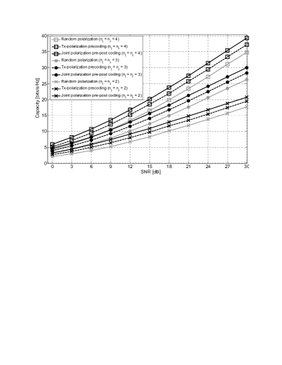
Figure 12: PR-MIMO channel capacity for the varying SNR in the scenarios of random Tx/Rx-polarization, Tx-polarization precoding, and joint polarization pre-post coding.

VII-B Simulations in PR-HS/MRT

In this section, we present simulation results focusing on the system performance when applying the proposed PR-HS/MRT scheme. The results include improved effective SNR, channel capacity and SER; the comparison of EW and global polarization reconfiguration schemes in terms of performance and selected Tx antenna indices; and verification of the theoretically derived SER in PR-HS/MRT via Monte-Carlo simulations. Unless otherwise stated, following system parameters will be used: $\bar{\Gamma}={\rm 20~{}dB},N_{t}=8$ and $N_{r}=2$ (MRC).

Figure 13: cdf curves of channel capacity for PR-HS/MRT with EW and global polarization reconfiguration schemes, conventional HS/MRT (Random Polarization), upper and lower bounds; with a variety of $L_{t}$.

Simulation results in Fig. 13 show the impact of PR-HS/MRT schemes on the channel capacity. Regardless of the number of selected Tx antenna elements, $L_{t}$, the proposed PR-HS/MRT schemes outperform the conventional HS/MRT without polarization reconfiguration,i.e., the case of Random Polarization in the legend of Fig. 13, by around 1 bit/s/Hz. Further, it is verified that EW polarization reconfiguration (Scheme-1) has better performance than global polarization reconfiguration (Scheme-2). However, the difference in performance decreases as $L_{t}$ increases. Hence, global polarization reconfiguration can also be a good suboptimal scheme considering the lower complexity and computation time than those of EW polarization reconfiguration, in particular, when $L_{t}\geq 4$ in the scenario of Fig. 13.

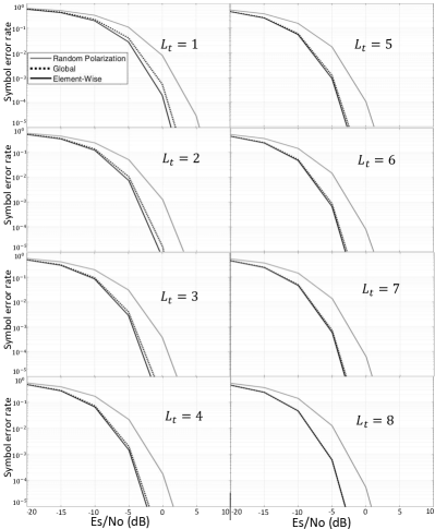
Figure 14: SER curves for PR-HS/MRT with EW and global polarization reconfiguration schemes and conventional HS/MRT (random polarization); with a variety of $L_{t}$..

Effective SER in PR-HS/MRT is also significantly lower than that in conventional HS/MRT, showing approximately 3 dB SNR gain to for $10^{-3}$ SER in every case of $L_{t}$, as described in Fig. 14. The SER curves are based on the analytical result in (65) considering QPSK modulation as a baseline. Besides, the difference in SER performance between EW and global polarization reconfiguration schemes is inconsiderable for a variety of $L_{t}$ in the scenario of Fig. 14. This is not surprising, given the straigthforward mapping between SNR and SER for the chosen modulation.

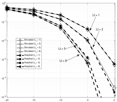
Figure 15: Validation of analytical SER curves via Monte-Carlo simulation

Monte-Carlo simulation results in Fig. 15 validate the analytical SER curves based on (65). SER curves are generated via Monte-Carlo simulation, where $10^{7}$ randomly generated symbols are transmitted based on PR-HS/MRT at the Tx, and MRC at the Rx. The scenarios of $L_{t}=1,2,5$ and $8$ are considered, and SER curves resulted in Monte-Carlo simulation shows good agreement with the analytical ones with with average SER.

Another observation of the selected Tx antenna indices in PR-HS/MRT and conventional HS/MRT, is given in Tables I – III. Even for a set of selected Tx antenna elements based on the conventional HS/MRT, the channel capacity and SER performance is improved via joint polarization pre-post coding after the selection. However, that selection of Tx antenna elements is different from the selection based on the proposed PR-HS/MRT. Moreover, selected antenna indices in EW polarization reconfigurable scheme is also different from those in global polarization reconfigurable scheme. Tables I – III illustrate the selected Tx antenna indices in 10 independent channel realizations for $L_{t}=1,4$ and $6$.

The conventional HS/MRT scheme does not show full-matching of selected antenna indices with any of two PR-HS/MRT schemes. On the other hand, the two PR-HS/MRT schemes, i.e., EW and global polarization reconfiguration, have a considerable number of cases in which their selected antenna indices fully match. As described in Tables I – III, the greater $L_{t}$ is, the more selected antenna indices are matched between proposed two PR-HS/MRT schemes. It is worth emphasizing that estimation of optimal polarization vectors before the hybrid antenna selection stage is inevitable to have full benefit of joint polarization pre-post coding.

Random	G	EW	Matching Index
7	3	4	0
1	5	4	0
6	1	7	0
6	4	4	1
2	4	7	0
5	6	6	1
7	5	8	0
7	4	4	1
3	2	7	0
3	4	4	1

TABLE I: Selected Tx Antenna Index when $L_{t}=1$

Random	G	EW	Matching Index
1 3 7 8	1 3 4 8	1 3 4 8	4
1 2 5 8	2 3 5 8	2 3 5 8	4
3 5 6 7	5 6 7 8	1 3 6 7	2
1 2 3 8	1 3 5 7	1 3 5 8	3
3 4 7 8	2 3 5 8	1 3 5 8	3
2 5 6 8	1 2 4 6	2 4 6 8	3
1 4 5 8	1 4 5 6	2 4 5 6	3
1 2 5 8	1 5 7 8	1 3 5 8	3
2 3 5 8	2 3 4 6	2 3 4 6	4
1 3 6 7	1 3 4 8	1 3 4 5	3

TABLE II: Selected Tx Antenna Index when $L_{t}=4$

Random	G	EW	Matching Index
1 2 3 4 7 8	1 2 3 5 6 7	1 2 3 5 6 7	6
1 3 5 6 7 8	1 3 5 6 7 8	1 3 5 6 7 8	6
1 3 4 5 7 8	1 2 4 5 7 8	1 2 3 4 7 8	5
2 3 4 5 6 8	1 2 3 5 6 7	1 2 3 4 7 8	4
1 2 3 4 7 8	2 3 4 6 7 8	2 3 4 6 7 8	6
1 3 4 5 7 8	1 2 4 5 6 7	1 2 4 5 6 7	6
1 2 4 6 7 8	1 3 4 6 7 8	1 2 4 6 7 8	5
2 3 4 5 6 8	1 2 3 5 6 8	1 2 3 5 6 8	6
1 2 3 4 5 7	1 2 3 6 7 8	2 3 4 5 7 8	4
1 2 5 6 7 8	2 3 4 5 6 7	2 3 4 5 6 7	6

TABLE III: Selected Tx Antenna Index when $L_{t}=6$

VIII Conclusion

In this paper, we proposed several novel schemes to support PR-MIMO spatial multiplexing and PR-HS/MRT whose system is composed of multiple polarization reconfigurable antenna elements at both the Tx and Rx. In the proposed iterative joint polarization pre-post coding, the local optimum usually reached the global optimum of Tx/Rx-polarization vectors within five iterations. The proposed method offers an energy-efficient as well as cost-efficient method to significantly increase channel capacity in PR-MIMO spatial multiplexing. Furthermore, we proposed two PR-HS/MRT schemes, i.e., EW and global polarization reconfiguration, and both schemes remarkably outperformed the conventional HS/MRT without polarization reconfigurable antennas. The theoretical analysis along with extensive simulation results demonstrate the good performance of the schemes proposed in this paper.

Appendix A Expectation and Variance of $Y=\cos\Theta$, $Y=\sin\Theta$ and $h^{\rm eff}_{ij}$

To find the expectation and variance of $Y=\cos{\Theta}$ and $X=\sin{\Theta}$, we start from (49). The expectation is found by solving the integral

$$E[Y]=\dfrac{1}{\pi}\int_{-1}^{1}\dfrac{dy}{\sqrt{1-y^{2}}}.$$ (66)

To solve, we substitute $u=1-y^{2}$, $du=-2ydy$ and $dy=\dfrac{1}{-2x}du$. Therefore,

$$E[Y] = \dfrac{1}{2\pi}\int\dfrac{1}{\sqrt{u}}du$$

$$= \dfrac{1}{2\pi}\sqrt{u}=\bigg{[}\dfrac{1}{2\pi}\sqrt{1-y^{2}}\bigg{]}\begin{matrix}1\\ -1\end{matrix}$$

$$= 0~{}.$$

We find variance by solving the integral

$$Var(Y) = \int_{-\infty}^{\infty}y^{2}f_{Y}(y)dy-\big{(}E[Y]\big{)}^{2}$$

$$= \dfrac{1}{\pi}\int_{-1}^{1}y^{2}\dfrac{1}{\sqrt{1-y^{2}}}dy~{}.$$

The second term of (A) disappears because expectation is 0. Substitute $y=\sin{u}$, $dy=\cos{u}~{}du$, and $u=\arcsin{y}$,

$$Var(Y) = \dfrac{1}{\pi}\int\dfrac{\sin^{2}{u}}{\sqrt{1-\sin^{2}{u}}}\cos{u}~{}du$$

$$= \dfrac{1}{\pi}\int\dfrac{\sin^{2}{u}}{\cos{u}}\cos{u}~{}du$$

$$= \dfrac{1}{2\pi}\int 1-\cos{2u}du$$

$$= \dfrac{1}{2\pi}u-\dfrac{1}{4\pi}\sin{2u}=\dfrac{1}{2\pi}(u-\sin{u}\cos{u})$$

$$= \dfrac{1}{2\pi}\bigg{(}\arcsin(y)-y\sqrt{1-y^{2}}\bigg{)}\begin{matrix}1\\ -1\end{matrix}$$

$$Var(Y) = \dfrac{1}{2}~{}.$$

To find $Var(h^{\rm eff}_{ij})$, we start from (43)

$$h_{ij}^{\rm eff} = \vec{p}^{~{}T}_{{\rm Rx},i}\begin{bmatrix}h^{\rm vv}_{ij}&h^{\rm vh}_{ij}\\ h^{\rm hv}_{ij}&h^{\rm hh}_{ij}\end{bmatrix}\vec{p}_{{\rm Tx},j}~{}~{}~{}~{}~{}~{}~{}~{}~{}~{}~{}~{}~{}~{}~{}~{}~{}~{}~{}~{}$$ (70)

$$= h^{\rm vv}_{ij}\cos(\theta_{j})\cos(\theta_{i})+h^{\rm hv}_{ij}\sin(\theta_{i})\cos(\theta_{j})$$

$$+h^{\rm vh}_{ij}\cos(\theta_{i})\sin(\theta_{j})+h^{\rm hh}_{ij}\sin(\theta_{j})\sin(\theta_{i})$$

$$= \beta_{1}+\beta_{2}+\beta_{3}+\beta_{4}~{}.$$

Therefore, the variance is

$$Var(h^{\rm eff}_{ij}) = E\big{[}(\beta_{1}+\beta_{2}+\beta_{3}+\beta_{4})^{2}\big{]}$$

$$-\bigg{(}E[\beta_{1}+\beta_{2}+\beta_{3}+\beta_{4}]\bigg{)}^{2}~{}.$$

All $\beta_{i}$’s are independent from each other; hence second term is addition of expectations of each $\beta_{i}$’s. Since they are zeros, they are eliminated from the equation.

When first term is foiled, it consists of squares and cross terms of $\beta_{i}$’s. The cross terms cancel out because elements of polarization basis matrix are independent from each other. Therefore, the variance is

$$Var(h^{\rm eff}_{ij}) = E\big{[}\beta^{2}_{1}+\beta^{2}_{2}+\beta^{2}_{3}+\beta^{2}_{4}\big{]}$$

$$= E[\beta^{2}_{1}]+E[\beta^{2}_{2}]+E[\beta^{2}_{3}]+E[\beta^{2}_{4}]$$

$$= Var(\beta_{1})+Var(\beta_{2})+Var(\beta_{3})+Var(\beta_{4})~{}.$$

Variance of product of independent random variable is product of variance of the random variables. Note that each three terms of $\beta_{i}$’s, where $i\in\{1,2,3,4\}$ are independent. Therefore, the variance of each $\beta_{i}$ is product of variances of three terms. Moreover, because each polarization-basis matrix element consists of real and imaginary part, we analyze the two parts separately. Both real and imaginary parts of all $\beta_{i}$’s, therefore, have variance of 1/8. Then, these variances are added to yield variance of $h^{\rm eff}_{ij}$, (50); that is 1/2 for both real and imaginary parts. Hence, real and imaginary part of $h^{\rm eff}_{ij}$ has means of 0 and variances of 1/2, which brings the element back to $H_{\rm o}$.

Appendix B Elaboration of Polarization Determinant Matrix

From (51),

$$|h^{\rm eff}_{11}|^{2}=\vec{p}_{{\rm Rx},1}^{~{}T}\big{(}H_{11}\vec{p}_{{\rm Tx},1}\vec{p}_{{\rm Tx},j}^{~{}T}H_{11}^{\dagger}\big{)}\vec{p}_{{\rm Rx},1}~{}~{}~{}~{}~{}~{}~{}~{}~{}~{}~{}~{}~{}~{}~{}~{}~{}~{}~{}~{}$$ (73)

$$=\big{[}\cos(\theta_{{\rm Rx},1})~{}\sin(\theta_{{\rm Rx},1})\big{]}\begin{bmatrix}h^{\rm PD}_{{\rm Rx},11}&h^{\rm PD}_{{\rm Rx},12}\\ h^{\rm PD}_{{\rm Rx},21}&h^{\rm PD}_{{\rm Rx},22}\end{bmatrix}\begin{bmatrix}\cos(\theta_{{\rm Rx},1})\\ \sin(\theta_{{\rm Rx},1})\end{bmatrix},$$

where

$$h^{\rm PD}_{{\rm Rx},11} = |h^{\rm vv}_{11}|^{2}\cos^{2}({\theta_{{\rm Tx},1}})$$

$$+h^{\rm vh}_{11}(h^{\rm vv}_{11})^{*}\sin(\theta_{{\rm Tx},1})\cos({\theta_{{\rm Tx},1}})$$

$$+h^{\rm vv}_{11}(h^{\rm vh}_{11})^{*}\sin(\theta_{{\rm Tx},1})\cos({\theta_{{\rm Tx},1}})$$

$$+|h^{\rm vh}_{11}|^{2}\sin^{2}({\theta_{{\rm Tx},1}})$$

$$h^{\rm PD}_{{\rm Rx},12} = h^{\rm vv}_{11}(h^{\rm hv}_{11})^{*}\cos^{2}({\theta_{{\rm Tx},1}})$$

$$+h^{\rm vh}_{11}(h^{\rm hv}_{11})^{*}\sin(\theta_{{\rm Tx},1})\cos({\theta_{{\rm Tx},1}})$$

$$+h^{\rm vv}_{11}(h^{\rm hh}_{11})^{*}\sin(\theta_{{\rm Tx},1})\cos({\theta_{{\rm Tx},1}})~{}~{}~{}~{}~{}~{}~{}~{}~{}~{}~{}~{}~{}~{}~{}~{}~{}~{}$$

$$+h^{\rm vh}_{11}(h^{\rm hh}_{11})^{*}\sin^{2}({\theta_{{\rm Tx},1}})$$

$$h^{\rm PD}_{{\rm Rx},21} = h^{\rm hv}_{11}(h^{\rm vv}_{11})^{*}\cos^{2}({\theta_{{\rm Tx},1}})$$

$$+h^{\rm hh}_{11}(h^{\rm vv}_{11})^{*}\sin(\theta_{{\rm Tx},1})\cos({\theta_{{\rm Tx},1}})$$

$$+h^{\rm hv}_{11}(h^{\rm vh}_{11})^{*}\sin(\theta_{{\rm Tx},1})\cos({\theta_{{\rm Tx},1}})$$

$$+h^{\rm hh}_{11}(h^{\rm vh}_{11})^{*}\sin^{2}({\theta_{{\rm Tx},1}})$$

$$h^{\rm PD}_{{\rm Rx},22} = |h^{\rm hv}_{11}|^{2}\cos^{2}({\theta_{{\rm Tx},1}})$$

$$+h^{\rm hh}_{11}(h^{\rm hv}_{11})^{*}\sin(\theta_{{\rm Tx},1})\cos({\theta_{{\rm Tx},1}})$$

$$+h^{\rm hv}_{11}(h^{\rm hh}_{11})^{*}\sin(\theta_{{\rm Tx},1})\cos({\theta_{{\rm Tx},1}})$$

$$+|h^{\rm hh}_{11}|^{2}\sin^{2}({\theta_{{\rm Tx},1}})~{}.$$

Note that the greatest values that we can acquire are the squared enveloped terms. The elements of polarization determinant matrices can be transformed into a different form with trigonometric properties. They result as

$$|h^{\rm eff}_{11}|^{2} = \dfrac{1}{4}\bigg{\{}|h^{\rm vv}_{11}|^{2}+|h^{\rm vh}_{11}|^{2}+|h^{\rm hv}_{11}|^{2}+|h^{\rm hh}_{11}|^{2}$$

$$+\cos{(2\theta_{{\rm Tx},1})}\big{[}|h^{\rm vv}_{11}|^{2}-|h^{\rm vh}_{11}|^{2}$$

$$+|h^{\rm hv}_{11}|^{2}-|h^{\rm hh}_{11}|^{2}\big{]}$$

$$+\sin{(2\theta_{{\rm Tx},1})}\big{[}h^{\rm vh}_{11}(h^{\rm vv}_{11})^{*}+h^{\rm vv}_{11}(h^{\rm vh}_{11})^{*}$$

$$+h^{\rm hh}_{11}(h^{\rm hv}_{11})^{*}+h^{\rm hv}_{11}(h^{\rm hh}_{11})^{*}\big{]}\bigg{\}}$$

$$+\dfrac{1}{4}\cos{(2\theta_{{\rm Rx},1})}\bigg{\{}|h^{\rm vv}_{11}|^{2}+|h^{\rm vh}_{11}|^{2}$$

$$+|h^{\rm hv}_{11}|^{2}+|h^{\rm hh}_{11}|^{2}$$

$$+\cos{(2\theta_{{\rm Tx},1})}\big{[}|h^{\rm vv}_{11}|^{2}-|h^{\rm vh}_{11}|^{2}~{}~{}~{}~{}~{}~{}~{}~{}~{}~{}~{}~{}~{}~{}~{}~{}~{}~{}~{}~{}~{}$$

$$+|h^{\rm hv}_{11}|^{2}-|h^{\rm hh}_{11}|^{2}\big{]}$$

$$+\sin{(2\theta_{{\rm Tx},1})}\big{[}h^{\rm vh}_{11}(h^{\rm vv}_{11})^{*}+h^{\rm vv}_{11}(h^{\rm vh}_{11})^{*}$$

$$+h^{\rm hh}_{11}(h^{\rm hv}_{11})^{*}+h^{\rm hv}_{11}(h^{\rm hh}_{11})^{*}\big{]}\bigg{\}}$$

$$+\dfrac{1}{4}\sin{(2\theta_{{\rm Rx},1})}\bigg{\{}h^{\rm vh}_{11}(h^{\rm vv}_{11})^{*}+h^{\rm vv}_{11}(h^{\rm vh}_{11})^{*}$$

$$+h^{\rm hh}_{11}(h^{\rm hv}_{11})^{*}+h^{\rm hv}_{11}(h^{\rm hh}_{11})^{*}$$

$$+\cos{(2\theta_{{\rm Tx},1})}\big{[}h^{\rm vh}_{11}(h^{\rm vv}_{11})^{*}-h^{\rm vv}_{11}(h^{\rm vh}_{11})^{*}$$

$$+h^{\rm hh}_{11}(h^{\rm hv}_{11})^{*}-h^{\rm hv}_{11}(h^{\rm hh}_{11})^{*}\big{]}$$

$$+\sin{(2\theta_{{\rm Tx},1})}\big{[}h^{\rm hh}_{11}(h^{\rm vv}_{11})^{*}+h^{\rm hv}_{11}(h^{\rm vh}_{11})^{*}$$

$$+h^{\rm vh}_{11}(h^{\rm hv}_{11})^{*}+h^{\rm hv}_{11}(h^{\rm hh}_{11})^{*}\big{]}\bigg{\}}~{}.$$

Depending on the channel condition, squared envelopes of elements of polarization-basis matrix are maximized with optimal values of $\theta_{{\rm Tx},j}$ and $\theta_{{\rm Rx},i}$ in each iteration.

$|h^{\rm eff}_{11}|^{2}$ consists of four squared envelope of the elements in polarization-basis matrix, i.e., $|h^{\rm vv}_{11}|^{2}$, $|h^{\rm vh}_{11}|^{2}$, $|h^{\rm hv}_{11}|^{2}$ and $|h^{\rm hh}_{11}|^{2}$. Besides, $|h^{\rm eff}_{11}|^{2}$ includes cross-term products between the elements in polarization-basis matrix. Squared envelope terms outcome higher values than that of the product of the cross terms; therefore, we focus on utilizing the squared envelope terms rather than the cross terms. Each aforementioned squared envelope terms follow chi-square distribution with 2 degrees of freedom; hence, summing them will result degrees of freedom up to 8. However, the four terms are multiplied by one fourth of $\cos(2\theta_{{\rm Tx},1})$ and one fourth of $\cos(2\theta_{{\rm Rx},1})$; therefore, each four squared envelope term will be multiplied by a weight less than unity. The weighted terms are then summed up at the end. Tx and Rx polarization angles are adjusted to yield greater squared envelope terms. Since squared envelope terms have weights less than unity and are superimposed, distribution will not always fit to degrees of freedom of an integer. Such case is represented in Fig. 5.

References

- [1] S.-C. Kwon and A. F. Molisch, “Capacity maximization with polarization-agile antennas in the MIMO communication system,” Proc. IEEE Global Telecommun. Conf., pp. 1–6, Dec. 2015.
- [2] P. Oh and S. Kwon, “Multi-polarization superposition beamforming with XPD-aware transmit power allocation,” Proc. IEEE Veh. Technol. Conf., pp. 1–6, Dec. 2020.
- [3] J. Zhang, K. J. Kim, A. A. Glazunov, Y. Wang, L. Ding, and J. Zhang, “Generalized polarization-space modulation,” IEEE Trans. Commun., vol. 68, no. 1, pp. 258–273, Jan. 2020.
- [4] A. Sousa de Sena, D. Benevides da Costa, Z. Ding, and P. H. J. Nardelli, “Massive MIMO-NOMA networks with multi-polarized antennas,” IEEE Trans. Wireless Commun., vol. 18, no. 12, pp. 5630–5642, 2019.
- [5] L. A. Gutierrez, S. An, S. Kwon, and H. G. Yeh, “Novel approach of spatial modulation: Polarization-aware OFDM subcarrier allocation,” Proceedings of IEEE Green Energy and Smart Systems Conference (IGESSC), 2020, pp. 1–6, 2020.
- [6] K. Satyanarayana, T. Ivanescu, M. El-Hajjar, P. . Kuo, A. Mourad, and L. Hanzo, “Hybrid beamforming design for dual-polarised millimetre wave MIMO systems,” IET Electronics Letters, vol. 54, no. 22, pp. 1257–1258, 2018.
- [7] X. Zhang, B. Zhang, and D. Guo, “Performance of poly-polarization multiplexing in narrow-band wireless communication aided by pre-compensation and multi-notch OPPFs,” IEEE Commun. Let., vol. 6, no. 4, pp. 478–481, Aug 2017.
- [8] G. Zafari, M. Koca, and H. Sari, “Dual-polarized spatial modulation over correlated fading channels,” IEEE Trans. Commun., vol. 65, no. 3, pp. 1336–1352, Mar. 2017.
- [9] P.-Y. Qin, S.-L. Chen, and Y. J. Guo, “A compound reconfigurable microstrip antenna with agile polarizations and steerable beams,” Proceedings of IEEE International Symposium on Antennas and Propagation (ISAP), 2017, pp. 1–2, 2017.
- [10] G. Wolosinski, V. Fusco, and O. Malyuskin, “2-bit polarisation agile antenna with high port decoupling,” Electronics Letters, vol. 52, no. 4, pp. 255–256, 2016.
- [11] B. Babakhani, S. K. Sharma, and N. R. Labadie, “A frequency agile microstrip patch phased array antenna with polarization reconfiguration,” IEEE Trans. Antennas Propag., vol. 64, no. 10, pp. 4316–4327, 2016.
- [12] H. Sun and S. Sun, “A novel reconfigurable feeding network for quad-polarization-agile antenna design,” IEEE Trans. Antennas Propag., vol. 64, no. 1, pp. 311–316, 2016.
- [13] L.-P. Cai and K.-K. M. Cheng, “Continuously tunable polarization agile antenna design using a novel varactor-only signal control device,” IEEE Trans. Antennas Propag., vol. 16, pp. 1147–1150, 2017.
- [14] Y.-J. Liao, H.-L. Lin et al., “Polarization reconfigurable eccentric annular ring slot antenna design,” IEEE Trans. Antennas Propag., vol. 63, no. 9, pp. 4152–4155, 2015.
- [15] S.-C. Kwon, “Optimal power and polarization for the capacity of polarization division multiple access channels,” in Proc. IEEE Global Telecommun. Conf., Dec. 2014, pp. 1–5.
- [16] J. Jootar, J.-F. Diouris, and J. Zeidler, “Performance of polarization diversity in correlated Nakagami-m fading channels,” IEEE Transactions on Vehicular Technology, vol. 55, no. 1, pp. 128–136, 2006.
- [17] Y. Deng, A. Burr, and G. White, “Performance of MIMO systems with combined polarization multiplexing and transmit diversity,” in Proc. IEEE Veh. Technol. Conf., vol. 2, May 2005, pp. 869–873.
- [18] R. Nabar, H. Bolcskei, V. Erceg, D. Gesbert, and A. Paulraj, “Performance of multiantenna signaling techniques in the presence of polarization diversity,” IEEE Trans. Sig. Proc., vol. 50, no. 10, pp. 2553–2562, Oct. 2002.
- [19] S.-C. Kwon and G. Stüber, “Polarization division multiple access on NLoS wide-band wireless fading channels,” IEEE Trans. Wireless Commun., vol. 13, no. 7, pp. 3726–3737, Jul. 2014.
- [20] S.-C. Kwon, “Geometrical theory, modeling and applications of channel polarization,” Ph.D. Thesis, Georgia Institute of Technology, pp. 1–128, 2014.
- [21] M. R. Andrews, P. P. Mitra, and R. deCarvalho, “Tripling the capacity of wireless communications using electromagnetic polarization,” Nature, vol. 409, pp. 316–318, Jan. 2001.
- [22] V. Erceg, P. Soma, D. Baum, and S. Catreux, “Multiple-input multiple-output fixed wireless radio channel measurements and modeling using dual-polarized antennas at 2.5 GHz,” IEEE Trans. Wireless Commun., vol. 3, no. 6, pp. 2288 – 2298, Nov. 2004.
- [23] M. Shafi, M. Zhang, A. Moustakas, P. Smith, A. Molisch, F. Tufvesson, and S. Simon, “Polarized MIMO channels in 3-D: Models, measurements, and mutual information,” IEEE J. Sel. Areas Commun., vol. 24, no. 3, pp. 514–527, Mar. 2006.
- [24] M. Landmann, K. Sivasondhivat, J.-I. Takada, I. Ida, and R. Thoma, “Polarisation behaviour of discrete multipath and diffuse scattering in urban environments at 4.5 GHz,” EURASIP J. Wireless Commun. Netw., no. 1, p. 60, Jan. 2007 Article ID 57980.
- [25] S.-C. Kwon and G. L. Stüber, “Geometrical theory of channel depolarization,” IEEE Trans. Veh. Technol., vol. 60, no. 8, pp. 3542–3556, Oct. 2011.
- [26] D. Landon and C. Furse, “Recovering handset diversity and MIMO capacity with polarization-agile antennas,” IEEE Trans. Antennas Propag., vol. 55, no. 11, pp. 3333–3340, Nov 2007.
- [27] O. Karabey, S. Bildik, S. Bausch, S. Strunck, A. Gaebler, and R. Jakoby, “Continuously polarization agile antenna by using liquid crystal-based tunable variable delay lines,” IEEE Trans. Antennas Propag., vol. 61, no. 1, pp. 70–76, Jan 2013.
- [28] P. Oh and S. Kwon, “Multi-polarization superposition beamforming with xpd-aware transmit power allocation,” in 2020 IEEE 92nd Vehicular Technology Conference (VTC2020-Fall), 2020, pp. 1–6.
- [29] A. Molisch, M. Win, and J. Winters, “Reduced-complexity transmit/receive-diversity systems,” IEEE Transactions on Signal Processing, vol. 51, no. 11, pp. 2729–2738, 2003.
- [30] M. Win and J. Winters, “Virtual branch analysis of symbol error probability for hybrid selection/maximal-ratio combining in Rayleigh fading,” IEEE Transactions on Communications, vol. 49, no. 11, pp. 1926–1934, 2001.
- [31] ——, “Analysis of hybrid selection/maximal-ratio combining in Rayleigh fading,” in 1999 IEEE International Conference on Communications (Cat. No. 99CH36311), vol. 1, 1999, pp. 6–10 vol.1.
- [32] D. Gore, R. Heath, and A. Paulraj, “Transmit selection in spatial multiplexing systems,” IEEE Communications Letters, vol. 6, no. 11, pp. 491–493, 2002.
- [33] A. Molisch, M. Win, Y.-S. Choi, and J. Winters, “Capacity of mimo systems with antenna selection,” IEEE Transactions on Wireless Communications, vol. 4, no. 4, pp. 1759–1772, 2005.
- [34] V. R. Anreddy and M. A. Ingram, “Wlc11-6: Antenna selection for compact dual-polarized MIMO systems with linear receivers,” in IEEE Globecom 2006, 2006, pp. 1–6.
- [35] A. Habib, “Multiple polarized MIMO with antenna selection,” in 2011 18th IEEE Symposium on Communications and Vehicular Technology in the Benelux (SCVT), 2011, pp. 1–8.
- [36] A. Molisch and M. Win, “MIMO systems with antenna selection,” IEEE Microwave Magazine, vol. 5, no. 1, pp. 46–56, Mar 2004.
- [37] A. F. Molisch, Wireless Communications, 2nd ed. Wiley and IEEE, 2010.
- [38] D. Tse and P. Viswanath, Fundamentals of Wireless Communication, 1st ed. Cambridge, 2005.
- [39] G. Strang, Linear Algebra and Its Applications, 4th ed. Thomson Learning, Inc., 2005.