Dirac materials under linear polarized light: quantum wave function evolution and topological Berry phases as classical charged particles trajectories under electromagnetic fields

Abstract

The response of electrons under linearly polarized light in Dirac materials as borophene or graphene is analyzed in a continuous wave regime for an arbitrary intense field. Using a rotation and a time-dependent phase transformation, the wave function evolution is shown to be governed by a spinor-component decoupled Whittaker-Hill equation. The numerical solution of these equations enables to find the quasienergy spectrum. For borophene it reveals a strong anisotropic response. By applying an extra unitary transformation, the wave functions are proven to follow an Ince equation. The evolution of the real and imaginary parts of the wave function is interpreted as the trajectory of a classical charged particle under oscillating electric and magnetic field. The topological properties of this forced quantum system are studied using this analogy. In particular, in the adiabatic driving regime, the system is described with an effective Matthieu equation while in the non-adiabatic regime the full Whittaker-Hill equation is needed. From there, it is possible to separate the dynamical and Berry phase contributions to obtain the topological phase diagram due to the driving. Therefore, a different path to perturbation theory is developed to obtain time-driven topological phases.

Keyword:

Dirac materials, topological phases, time driven systems, graphene, borophene

1 Introduction

The possibility of inducing a nontrivial topology in condensed matter systems by means of an electromagnetic drive has been the subject of many research works in recent years [1, 2, 3, 4, 5, 6, 7, 8, 9, 10], some of which have focused in Dirac systems such as graphene [11, 12, 13, 14, 15, 16, 17, 18].

More recently, two dimensional (2D) boron allotropes, also called borophenes, exhibiting Dirac cones have attracted attention due to their remarkable anisotropic properties [19, 20, 21, 22]. In a series of previous works we studied the effects of linear[23] and elliptical[24, 25] polarized electromagnetic fields in borophene. The focus of such works was in finding the quasienergy spectrum, the associated photo currents and induced transitions, useful to design 2D electronic devices [26]. In the present work, we exploit these results and others [27, 28, 9] to study the wave function evolution and the topology induced by the interplay between an electromagnetic drive and the electrons in a Dirac system. To do so, we introduce a drive to the continuum model for a general tilted Dirac Hamiltonian. Then we use the Floquet formalism to establish the equivalence between the quantum wave function evolution and the motion of a classical charged particle in a time-dependent electromagnetic field. This is achieved through a unitary transformation that turns the time-dependent Schrödinger equation into a Ince differential equation. The advantage of such formalism is that we can use previous studies on the trajectories of particles under time dependent electromagnetic drive [29] as well as from studies of differential equations with time-dependent coefficients [30, 31]. In particular, the quantum spectrum is given by the stability charts of Mathieu’s and Hill’s equations and its generalizations [30]. Such equations occurs in electromagnetism, mechanics, cooling of ions, aerodynamics, marine research, biomedical engineering, celestial mechanics and general relativity [32]. Thus, the induced topological phases in the quantum problem are discussed at different regimes from the perspective of classical orbital precession.

2 Dirac materials subject to electromagnetic fields

In this section we address the model and summarize previous results concerning the Floquet theory and the quasienergy spectrum for time-driven Dirac materials [33, 24, 34].

2.1 Isotropic, anisotropic and tilted Dirac materials

The most general, low-energy Dirac Hamiltonian close to one of the Dirac points, is given by [21, 35, 23, 36]

$$\hat{H}=\hbar v_{t}k_{y}\hat{\sigma}_{0}+\hbar\left[v_{x}k_{x}\hat{\sigma}_{x}+v_{y}k_{y}\hat{\sigma}_{y}\right],$$ (1)

where $k_{x}$ and $k_{y}$ are the components of the two-dimensional momentum vector $\bm{k}$, $\hat{\sigma}_{x}$ and $\hat{\sigma}_{y}$ are the Pauli matrices, and $\hat{\sigma}_{0}$ is the $2\times 2$ identity matrix. This Hamiltonian describes, for example, $8-Pmmn$ borophene. The three velocities in the anisotropic $8-Pmmn$ borophene Dirac Hamiltonian (1) are given by $v_{x}=0.86v_{F}$, $v_{y}=0.69v_{F}$ and $v_{t}=0.32v_{F}$ where $v_{F}=10^{6}\,m/s$ [21] is the Fermi velocity. In Eq. (1), the last two terms give rise to the familiar form of the kinetic energy leading to the Dirac cone and the first one tilts the Dirac cone in the $y$ direction. These two features are contained in the energy dispersion relation[24]

$$E_{\eta,k}=\left(\frac{v_{t}}{v_{y}}\right)\tilde{k}_{y}+\nu\epsilon,$$ (2)

where

$$\epsilon_{\bm{k}}=\sqrt{\tilde{k}_{x}^{2}+\tilde{k}_{y}^{2}},$$ (3)

and $\nu=\pm 1$ is the band index. In Eq. (2), we used the set of renormalized moments $\tilde{k}_{x}=\hbar v_{x}k_{x}$, $\tilde{k}_{y}=\hbar v_{y}k_{y}$. The corresponding free electron wave function is,

$$\psi_{\nu}(\bm{k})=\frac{1}{\sqrt{2}}\left[\begin{array}[]{c}1\\ \nu\exp(i\theta_{\bm{k}})\end{array}\right],$$ (4)

where $\theta_{\bm{k}}=\tan^{-1}(\tilde{k}_{y}/\tilde{k}_{x})$. The case of graphene can be recovered by setting $v_{t}=0$ and $v_{x}=v_{y}=v_{F}$ and for non-uniform strained graphene requires $v_{t}=0$ and $v_{x}\neq v_{y}$.

2.2 Linearly polarized waves and Whittaker-Hill equation

Now we consider a charge carrier, described by the two-dimensional anisotropic Dirac Hamiltonian, subject to an electromagnetic wave that propagates along a direction perpendicular to the surface of the crystal. The effects of the electromagnetic field are introduced in the Dirac Hamiltonian (1) through the Peierls substitution[33, 37] $\hbar\bm{k}\rightarrow\hbar\bm{k}-e\bm{A}$ where $\bm{A}=(A_{x},A_{y})$ is the vector potential of the electromagnetic wave. Adopting a gauge in which $\bm{A}$ only depends on time brings a significant simplification. The Hamiltonian (1) is thus transformed into [33, 37] ,

$$\hat{H}=\frac{v_{t}}{v_{y}}\left(\tilde{k}_{y}-ev_{y}A_{y}\right)\hat{\sigma}_{0}+\left(\tilde{k}_{x}-ev_{x}A_{x}\right)\hat{\sigma}_{x}+\left(\tilde{k}_{y}-ev_{y}A_{y}\right)\hat{\sigma}_{y}.$$ (5)

Assuming the electromagnetic wave to be linearly polarized and propagating along the $z$ direction, the vector potential can be written as

$$\bm{A}=\frac{E_{0}}{\Omega}\cos(\Omega t)\bm{\hat{r}},$$ (6)

where $\bm{\hat{r}}=(1,0)$ is the polarization vector, $E_{0}$ is the uniform amplitude of the electric field and $\Omega$ is the angular frequency of the electromagnetic wave. It is noteworthy that the field $\bm{A}$ is not quantized and is treated clasically. Thus, our results are only valid for quantum coherent field composed of a large number of photons. In the Schrödinger equation corresponding to (5),

$$i\hbar\frac{d}{dt}{\bm{\Psi}}(t)=\hat{H}(t){\bm{\Psi}}(t),$$ (7)

the two dimensional spinor can be expressed as $\bm{\Psi}(t)=\left(\Psi_{A}(t),\Psi_{B}(t)\right)^{\top}$, where $A$ and $B$ label the two sublattices. Formally, the solutions can be obtained from the time evolution operator $\hat{\mathcal{U}}(t)$ as,

$${\bm{\Psi}}(t)=\hat{\mathcal{U}}(t){\bm{\Psi}}(0).$$ (8)

Due to the time periodicity of the Hamiltonian $\hat{H}(t)=\hat{H}(t+T)$ where $T=2\pi/\Omega$, solutions must comply with the Floquet theorem [33, 38] that states that the evolution operator must have the form

$$\hat{\mathcal{U}}(t)=\exp\left(-\frac{i}{\hbar}\hat{H}_{e}t\right)\hat{\mathcal{W}}(t),$$ (9)

where $\hat{\mathcal{W}}(t+T)=\hat{\mathcal{W}}(t)$ and $\hat{H}_{e}$ is called the effective Hamiltonian. The eigenvalues of $\hat{H}_{e}$ are the quasienergies of $\hat{H}(t)$

$$\mathcal{E}_{\eta,j,m}(\bm{k})=-\frac{\hbar\omega}{2\pi}\arg[u_{\eta,j}(\bm{k})]+m\hbar\omega,$$ (10)

where $u_{\eta,j}(\bm{k})$ are the two eigenvalues of $\hat{\mathcal{U}}(T)$, and $m=0,\pm 1,\pm 2,\dots$ and $j=1,2$ denote the Floquet zone and the band respectively [34].

The main challenge in deducing the wave function’s explicit form resides in unraveling the coupling between the spinor components $\Psi_{A}(t)$ and $\Psi_{B}(t)$ that arise from terms proportional to $\hat{\sigma}_{x}$ and $\hat{\sigma}_{y}$ in Eq. (5). To uncouple the spinor components we proceed as follows. First, to transform the non-diagonal $\hat{\sigma}_{x}$ matrix into $\hat{\sigma}_{z}$, we apply a $45^{\circ}$ rotation around the $y$ axis of the form [34],

$$\mathbf{\Psi}(t)=\exp\left[-i\left(\frac{\pi}{4}\right)\hat{\sigma}_{y}\right]\mathbf{\Phi}(t).$$ (11)

Substituting (11) into Eq. (7) we obtain

$$i\frac{d}{d\phi}\mathbf{\Phi}(\phi)=\frac{2}{\hbar\Omega}\left[\left(\frac{v_{t}}{v_{y}}\right)\tilde{k}_{y}\hat{\sigma}_{0}+\tilde{\Pi}_{x}\hat{\sigma}_{z}+\tilde{k}_{y}\hat{\sigma}_{y}\right]\mathbf{\mathbf{\Phi}}(\phi)\,,$$ (12)

where the only off-diagonal terms originate from $\hat{\sigma}_{y}$. In the foregoing equation, the scaled time is defined as $\phi=\Omega t/2$, the scaled momentum $\tilde{\Pi}_{x}=\tilde{k}_{x}-\zeta_{x}\cos(2\phi)$ and the frequency-weighted induced dipole moment is,

$$\zeta_{x}=\frac{ev_{x}E_{x}}{\Omega}.$$ (13)

The spinor components of $\mathbf{\Phi}(\phi)=\left(\Phi_{+}(\phi),\Phi_{-}(\phi)\right)^{\top}$ are given by $\Phi_{+}(\phi)=[\Psi_{A}(\phi)+\Psi_{B}(\phi)]/\sqrt{2}$ and $\Phi_{-}(\phi)=[\Psi_{A}(\phi)-\Psi_{B}(\phi)]/\sqrt{2}$. Second, the term proportional to $\hat{\sigma}_{0}$ in Eq. (12) is removed by adding a time-dependent phase to the wave function

$$\mathbf{\Phi}(\phi)=\exp\left[-2i\left(\frac{v_{t}}{v_{y}}\right)\frac{\tilde{k}_{y}}{\hbar\Omega}\,\phi\,\hat{\sigma}_{0}\right]\bm{\chi}(\phi),$$ (14)

where $\bm{\chi}(\phi)=(\chi_{+1}(\phi),\chi_{-1}(\phi))^{\top}$. Finally, after inserting Eq. (14) into Eq. (12), differentiating both sides with respect to $\phi$ and using Eq. (12) to leave out the first order derivative, the resulting differential equation takes the form of a Whittakker-Hill equation [39, 34]

$$\bm{\chi}^{\prime\prime}(\phi)+\mathbbm{F}(\phi)\bm{\chi}(\phi)=0\,,$$ (15)

where the matrix $\mathbbm{F}(\phi)$ is defined as

$$\mathbbm{F}(\phi)=\left[a_{\bm{k}}+q_{1}\cos(2\phi)+q_{2}\cos(4\phi)\right]\hat{\sigma}_{0}+iq_{3}\sin(2\phi)\hat{\sigma}_{z}.$$ (16)

The Hill equation parameters are defined as,

$$a_{\bm{k}}=\left(\frac{2\epsilon_{\bm{k}}}{\hbar\Omega}\right)^{2}+2q_{0}^{2},$$ (17)

$$q_{1}=-8q_{0}\left(\frac{\tilde{k}_{x}}{\hbar\Omega}\right),$$ (18)

$$q_{2}=2q_{0}^{2},$$ (19)

$$q_{3}=4q_{0},$$ (20)

where

$$q_{0}=\frac{\zeta_{x}}{\hbar\Omega}=\frac{ev_{x}E_{x}}{\hbar\Omega^{2}},$$ (21)

is the ratio between two characteristic energies of the system: the electric-field-induced dipole moment $ev_{x}/\Omega$ with energy $ev_{x}E_{x}/\Omega$ and the photon energy $\hbar\Omega$[40, 24]. Thereby, $\epsilon/\hbar\Omega$ is the ratio of the electron kinetic energy to the photon energy, $\zeta_{x}/\hbar\Omega$ is the ratio of the work done on the charged carriers by the electromagnetic wave to the photon energy and $\tilde{k}_{x}/\hbar\Omega$ is the ratio of the $x$ contribution of the electron kinetic energy to the photon energy.

Expressing (15) as a second order differential equation is quite advantageous for the calculations that follow. First, the evolution operator that propagates the state $\chi(\phi)$ in time must be diagonal since $\mathbbm{F}(\phi)$ is solely composed of the diagonal matrices $\hat{\sigma}_{0}$ and $\hat{\sigma}_{z}$. As a consequence of this, the scalar differential equations for the $\chi_{+1}(\phi)$ and $\chi_{-1}(\phi)$ spinor components decouple. Moreover, the differential equation for the $\chi_{-1}(\phi)$ component turns out to be the complex conjugate of the one for $\chi_{+1}(\phi)$. Both differential equations may be summarized by

$$\chi_{\eta}^{\prime\prime}(\phi)+\left[a_{\bm{k}}+q_{1}\cos(2\phi)+q_{2}\cos(4\phi)+i\eta q_{3}\sin(2\phi)\right]\chi_{\eta}(\phi)=0,$$ (22)

where $\eta=\pm 1$. In principle, we can obtain the solution for $\eta=-1$ from the $\eta=1$ solution. This is done by making the replacement $\phi\rightarrow-\phi$ in Eq. (22), as $\eta\sin{2\phi}=\sin{2\eta\phi}$. The cosines and second derivative terms are not affected by a change of sign of $\phi$. Therefore, the solutions are related by,

$$\chi_{-1}(\phi)=\chi_{1}(-\phi).$$ (23)

However, in general the initial conditions on the first derivative of $\chi_{\eta}(\phi)$ are restricted by Eq. (12) and thus Eq. (23) can only be used for $\tilde{k}_{y}=0$.

We can also obtain a useful alternative expression to Eq. (22) by writing $\epsilon_{\bm{k}}$ in terms of the scaled moments,

$$\chi_{\eta}^{\prime\prime}(\phi)+4\bigg{[}\left(\frac{\tilde{k}_{x}}{\hbar\Omega}-q_{0}\cos(2\phi)\right)^{2}+\left(\frac{\tilde{k}_{y}}{\hbar\Omega}\right)^{2}+i\eta q_{0}\sin(2\phi)\bigg{]}\chi_{\eta}(\phi)=0.$$ (24)

In the previous equation, or Eq. (22), the spinor components are decoupled considerably simplifying the computation and the quasienergy spectrum analysis. Another gain of using this particular base is that $\chi_{+}(\phi)$ and $\chi_{-}(\phi)$ are the probability amplitudes of the valence and conduction bands, respectively.

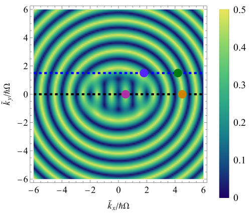
Figure 1: Density plot of quasienergy spectrum $\mathcal{E}_{\eta,j,m}-v_{t}\tilde{k}_{y}/(v_{y}\hbar\Omega)$ for $\eta=1$ and $m=0$ as a function of $\tilde{k}_{x}/\hbar\Omega$ and $\tilde{k}_{y}/\hbar\Omega$. The amplitude and frequency of the electromagnetic wave are $E_{x}=4.5\,$V/m and $\Omega=50\times 10^{9}\,$Hz. The horizontal dashed black and blue lines correspond to fixed values $\tilde{k}_{y}/\hbar\Omega=0$ and $\tilde{k}_{y}/\hbar\Omega=1.5$, respectively. The dots are the states that were chosen to produce the trajectories in Figs. 2 and 3.

In figure 1 we present the corresponding quasienergy spectrum obtained using a very powerful method developed in a previous work: the monodromy matrix method [25] for the CB $\eta=1$ and the Floquet zone $m=0$. This is equivalent to finding the stability regions of Eq. (22). Notice the two different regions in the spectrum. One is at the center where an American football ball-like shape is seen. The other, in the outer regions of the spectrum, exhibits concentric circles. Inside the ball, the energy of electrons is less than the energy of a photon and corresponds to a strong electromagnetic field regime. Outside the ball, the system can be considered in a weak interaction regime where the quasienergy spectrum is almost similar to the non-perturbed energy dispersion. In this case, the driving can be considered adiabatic. The condition that defines the crossover between the adiabatic and non-adiabatic regimes is thus given by the perimeter of the ball, i.e.,

$$\epsilon_{\bm{k}}\approx\zeta_{x}=\hbar\Omega q_{0}.$$ (25)

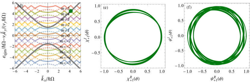
Figure 3: Quasienergy spectrum $\mathcal{E}_{\eta,j,m}-v_{t}\tilde{k}_{y}/v_{y}\hbar\Omega$ and the Floquet quantum wave real and imaginary part for the Wittaker-Hill and Ince equations. In panels (a) and (d), we show the quasienergy spectra as a function of the momentum $\tilde{k}_{x}/\hbar\Omega$ using the fixed values $\tilde{k}_{y}/\hbar\Omega=0$ and $\tilde{k}_{y}/\hbar\Omega=1.5$ for $\eta=1,\,2$ and $m=0,\pm 1,...,\pm 5$ (Floquet zones), respectively. In these panels, the orange dot correspond to the state where $(\tilde{k}_{x}/\hbar\Omega,\,\,\mathcal{E}_{\eta,j,m}-v_{t}\tilde{k}_{y}/v_{y}\hbar\Omega)=(4.5,\,4.5)$ and the corresponding green dot is the state $(\tilde{k}_{x}/\hbar\Omega,\,\mathcal{E}_{\eta,j,m}-v_{t}\tilde{k}_{y}/v_{y}\hbar\Omega)=(4.2,\,4.49)$. The solid gray lines corresponds to the dispersion relation given by equation (3) for fixed $\tilde{k}_{x}/\hbar\Omega$ values mentioned above. In panels (b) and (c), we show the trajectories for the Whittaker-Hill and Ince equations for $\eta=1$ and $(\tilde{k}_{x}/\hbar\Omega,\,\,\mathcal{E}_{\eta,j,m}-v_{t}\tilde{k}_{y}/v_{y}\hbar\Omega)=(4.5,\,4.5)$, respectively. The panels (e) and (f) are the corresponding trajectories for $\eta=1$ and $(\tilde{k}_{x}/\hbar\Omega,\,\mathcal{E}_{\eta,j,m}-v_{t}\tilde{k}_{y}/v_{y}\hbar\Omega)=(4.2,\,4.49)$. In all these panels the value of amplitude and frequency of the electromagnetic wave are $E_{x}=4.85\,$V/m and $\Omega=50\times 10^{9}\,$Hz, corresponding to $q_{0}=2.35$. Observe how trajectories with $\tilde{k}_{y}/\hbar\Omega=0$ describe circles in agreement with Eq. (26).

Let us then consider three different regimes: the adiabatic ($ev_{x}E_{x}/\hbar\Omega^{2}<1$), the non-adiabatic ($ev_{x}E_{x}/\hbar\Omega^{2}>1$) and the transitional ($ev_{x}E_{x}/\hbar\Omega^{2}\approx 1$) regimes. In Figs. 2(b), 2(e), and 3(b), we present the evolution of the real and imaginary parts of the first spinor component $\chi_{1}(\phi)$ for states chosen at different points of the Borophene’s quasienergy spectrum. These states, indicated with dots in Fig. 1, correspond to the four most representative cases listed below:

1. Adiabatic regime with $\tilde{k}_{y}\neq 0$ (green dot),

2. Non-adiabatic regime with $\tilde{k}_{y}=0$ (purple dot),

3. Non-adiabatic regime with $\tilde{k}_{y}\neq 0$ (blue dot),

4. Transitional regime with $\tilde{k}_{y}=0$ (orange dot).

The trajectories seen in Figs. 2(b), 2(e), 3(b), and 3(e) were obtained from a numerical simulation made by solving Eq. (22). As the initial state, we chose a band eigenstate of the time-independent problem. Since (22) is a second order differential equation, it requires an additional initial condition that comes from the first derivative of the wave function in Eq. (12). In Figs. 2(a), 2(d), 3(a) and in 3(e) we indicate the chosen states in several quasi spectrum cross sections. The Floquet zone replicas are also tagged.

From Figs. 2(b), 2(e), 3(b), and 3(e), we observe that as the wave functions evolve their real and imaginary parts may either move along complex paths or even describe simple circular trajectories. In particular, in Figs. 2(b) and 3(c), the real and imaginary parts of the wave function describe circular paths. This can be understood from Eq. (24), or more directly from Eq. (12), as in this case $\tilde{k}_{y}=0$ the spinor components are decoupled right from the beginning and there is no need to go into the second derivative calculation. Thus, $\mathbf{\chi}(\phi)=(\chi_{+1}(\phi),\chi_{-1}(\phi))$ and the solution is,

$$\chi_{\eta}(\phi)=\chi_{\eta}(0)\exp\left[-2i\eta\int_{0}^{\phi}\left(q_{0}\cos(2\phi^{\prime})-\frac{\tilde{k}_{x}}{\hbar\Omega}\right)d\phi^{\prime}\right],$$ (26)

or using that in this case $\epsilon_{\bm{k}}=\tilde{k_{x}}$, we obtain that,

$$\chi_{\eta}(t)=\chi_{\eta}(0)\exp\left[-i\eta\left(q_{0}\sin{(2\Omega t)}-\frac{2\epsilon_{\bm{k}}t}{\hbar}\right)\right].$$ (27)

The real and imaginary parts of this solution describe the circular paths shown in Figs. 2(b) and 3(b). What is remarkable here is that Eq. (27) holds in the non-adiabatic, the adiabatic and the transitional regime, i.e., it covers items 2 and 4 of the list of most representative cases. As we will see in the following section, this allows to characterize the Berry phase in a simple way.

Now let us return to the case where in Eq. (18) $\tilde{k}_{x}\neq 0$ and $\tilde{k}_{y}\neq 0$ but $q_{1}\gg q^{2}_{0}$. Under these conditions the solution of Eq. (18) requires setting $\tilde{k}_{x}\gg q_{0}\hbar\Omega$ from where $\epsilon\gg\hbar\Omega q_{0}$. According to Eq. (25) such a case corresponds to states well inside the adiabatic regime. Using Eq. (19) we neglect $q_{2}$ and Eq. (24) takes the form

$$\chi_{\eta}^{\prime\prime}(\phi)+\left[a_{\bm{k}}+q_{1}\cos(2\phi)+i\eta q_{3}\sin(2\phi)\right]\chi_{\eta}(\phi)=0.$$ (28)

This is a generalized Matthieu equation [30], but if we further assume that $\tilde{k}_{x}\gg\hbar\Omega/2$ and therefore photons are far from inducing transitions, then Eq. (22) transforms into a simple Matthieu equation as $q_{1}\gg q_{0}$ giving

$$\chi_{\eta}^{\prime\prime}(\phi)+\left[a_{\bm{k}}+q_{1}\cos(2\phi)\right]\chi_{\eta}(\phi)=0.$$ (29)

This very well known equation describes a pendulum with time-driven variable length, or alternatively, an harmonic oscillator with natural frequency $\sqrt{a}a_{\bm{k}}$ with a periodically perturbed time-dependent spring constant variation $-q_{1}\cos(2\phi)$. The physical relevant solutions are given by a stability chart in the $a$ and $q_{1}$ parameter space, divided in forbidden and allowed regions[30]. Resonances appear around $\sqrt{a_{\bm{k}}}=n$ with $n$ integer. In this quantum context, the forbidden regions correspond to the spectral gaps as they represent non-physical runaway solutions. Each resonance defines the limit of the Floquet zone. Including the initial conditions, the solutions are given by,

$$\chi_{-}(\phi) = \frac{\mathcal{C}\left(a_{\bm{k}},-\frac{q_{1}}{2},\phi\right)}{\mathcal{C}\left(a_{\bm{k}},-\frac{q_{1}}{2},0\right)}-\frac{2i\left(\tilde{k}_{x}-q_{0}\right)\mathcal{S}\left(a_{\bm{k}},-\frac{q_{1}}{2},\phi\right)}{\Omega\mathcal{S}^{\prime}\left(a_{\bm{k}},-\frac{q_{1}}{2},0\right)},$$ (30)

$$\chi_{+}(\phi) = \frac{2\tilde{k}_{y}\mathcal{S}\left(a_{\bm{k}},-\frac{q_{1}}{2},\phi\right)}{\Omega\mathcal{S}^{\prime}\left(a_{\bm{k}},-\frac{q_{1}}{2},0\right)}.$$ (31)

where $\mathcal{C}(a_{\bm{k}},-q_{1}/2,\phi)$ and $\mathcal{S}(a_{\bm{k}},-q_{1}/2,\phi)$ are the Mathieu cosine and sine functions, respectively. The first derivatives of the Mathieu functions are $\mathcal{C}^{\prime}(a_{\bm{k}},-q_{1}/2,\phi)=d/d\phi\mathcal{C}(a_{\bm{k}},-q_{1}/2,\phi)$ and $\mathcal{S}^{\prime}(a_{\bm{k}},-q_{1}/2,\phi)=d/d\phi\mathcal{S}(a_{\bm{k}},-q_{1}/2,\phi)$. Aside from the initial conditions ensued by Eq. (12), in the previous equations we have also assumed that $\chi_{+}(0)=0$ and $\chi_{-}(0)=1$ which means that initially the electron is in the valence band. The quasienergies are obtained by using the Fourier expansion of such functions. This is a very interesting result as in the adiabatic regimen we have both the oscillator’s fundamental frequency and the oscillating drive’s frequency. As we will discuss, our results must be akin to those of Thouless concerning adiabatic phases and thus Berry topology. However, here we arrived to such result not by perturbation theory but from a non-perturbative approach. Moreover, our generalized Hill equation (22) allows to find extra contributions and explore non-adiabatic regimes.

Also, the previous analysis of particular cases opens the question whether if for $q_{3}\neq 0$ we can develop a suitable classical analogy to the quantum equations. This is the subject of the following section.

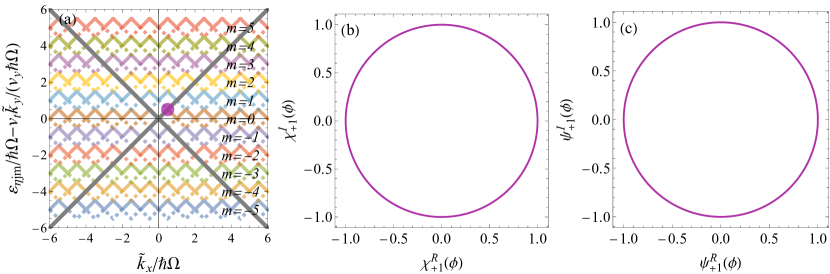
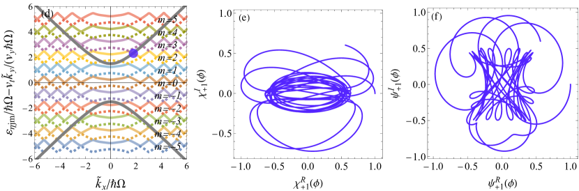
Figure 2: Quasienergy spectrum $\mathcal{E}_{\eta,j,m}-v_{t}\tilde{k}_{y}/v_{y}\hbar\Omega$ and the Floquet quantum wave real and imaginary part for the Wittaker-Hill and Ince equations. In panels (a) and (d), we show the quasienergy spectra as a function of the momentum $\tilde{k}_{x}/\hbar\Omega$ using the fixed values $\tilde{k}_{y}/\hbar\Omega=0$ and $\tilde{k}_{y}/\hbar\Omega=1.5$ for $\eta=1,\,2$ and $m=0,\pm 1,...,\pm 5$ (Floquet zones), respectively. In these panels, the purple dot correspond to the state where $(\tilde{k}_{x}/\hbar\Omega,\,\,\mathcal{E}_{\eta,j,m}-v_{t}\tilde{k}_{y}/v_{y}\hbar\Omega)=(0.50,\,0.50)$ and the corresponding blue dot is the state $(\tilde{k}_{x}/\hbar\Omega,\,\mathcal{E}_{\eta,j,m}-v_{t}\tilde{k}_{y}/v_{y}\hbar\Omega)=(1.79,\,2.31)$. The solid gray lines correspond to the dispersion relation given by equation (3) for fixed $\tilde{k}_{x}/\hbar\Omega$ values mentioned above. In panels (b) and (c), we show the trajectories for the Whittaker-Hill and Ince equations for $\eta=1$ and $(\tilde{k}_{x}/\hbar\Omega,\,\,\mathcal{E}_{\eta,j,m}-v_{t}\tilde{k}_{y}/v_{y}\hbar\Omega)=(0.5,\,0.50)$, respectively. The panels (e) and (f) are the corresponding trajectories for $\eta=1$ and $(\tilde{k}_{x}/\hbar\Omega,\,\mathcal{E}_{\eta,j,m}-v_{t}\tilde{k}_{y}/v_{y}\hbar\Omega)=(1.79,\,2.31)$. In all these panels the value of amplitude and frequency of the electromagnetic wave are $E_{x}=4.85\,$V/m and $\Omega=50\times 10^{9}\,$Hz, corresponding to $q_{0}=2.35$. Observe how trajectories with $\tilde{k}_{y}/\hbar\Omega=0$ describe circles in agreement with Eq. (26).

3 Ince equation: quantum wave functions as classical trajectories under electromagnetic fields

The previous section showed how a quantum wave function evolution of a time-driven system can be described in some particular cases by a simple classical problem. In this section we show how to fully extend the analogy to a classical system. In particular, we study the trajectories that arise when the Whittaker-Hill equation (15) is transformed into the Ince equation. Consider the following unitary transformation

$$\chi_{\eta}(\phi)=\exp\left[i\eta q_{0}\sin(2\phi)\right]\psi_{\eta}(\phi),$$ (32)

Substituting this last expression into Eq. (15), turns the Wittaker-Hill equation into a Ince equation for $\psi_{\eta}(\phi)$, i.e.,

$$\psi^{\prime\prime}_{\eta}(\phi)+if_{\eta}(\phi)\psi^{\prime}_{\eta}(\phi)+g(\phi)\psi_{\eta}(\phi)=0,$$ (33)

where

$$f_{\eta}(\phi)=\eta|q_{3}|\cos\left(2\phi\right),$$ (34)

$$g(\phi)=\left(\frac{2\epsilon_{\bm{k}}}{\hbar\Omega}\right)^{2}+q_{1}\cos(2\phi).$$ (35)

There are two advantages of the transformation given by Eq. (32). One is evident by comparing with Eq. (26), as it separates the contribution that comes from $\tilde{k}_{x}$ whenever $\tilde{k_{y}}=0$. But what is more important here is the possibility of finding a suitable classical analogy. Although this can be done in the Whitaker-Hill equation, the resulting fields are far from simple known physical cases. The solution of the Ince differential equation can be decomposed into its real part and its imaginary part, that is, $\psi_{\eta}(\phi)=\psi_{\eta}^{R}(\phi)+i\psi_{\eta}^{I}(\phi)$, and we find the following set of coupled differential equations

$$\frac{d^{2}}{d\phi^{2}}\psi_{\eta}^{R}(\phi)-f_{\eta}(\phi)\frac{d}{d\phi}\psi_{\eta}^{I}(\phi)+g(\phi)\psi^{R}_{\eta}(\phi)=0,$$ (36)

$$\frac{d^{2}}{d\phi^{2}}\psi_{\eta}^{I}(\phi)+f_{\eta}(\phi)\frac{d}{d\phi}\psi_{\eta}^{R}(\phi)+g(\phi)\psi^{I}_{\eta}(\phi)=0.$$ (37)

Let us know explore the classical analogy. We propose the following replacement $\psi^{R}_{\eta}(\phi)\rightarrow X(\phi)$, $\psi^{I}_{\eta}(\phi)\rightarrow Y(\phi)$. Notice that to keep the derivation simple, we drop $\eta$ and then quote the result for $\eta=-1$ at the end of the calculation. The resulting Ince equations are written as,

$$\frac{d^{2}X(\phi)}{d\phi^{2}}-f_{\eta}(\phi)\frac{d}{d\phi}Y(\phi)+g(\phi)X(\phi)=0,$$ (38)

$$\frac{d^{2}Y(\phi)}{d\phi^{2}}+f_{\eta}(\phi)\frac{d}{d\phi}X(\phi)+g(\phi)Y(\phi)=0.$$ (39)

Consider the problem of classical particle with mass $m$ and charge $Q$ moving in a plane under an electromagnetic field given by a radial time dependent electric field,

$$\mathbf{E(t)}=-\frac{g(t)}{Q}\mathbf{r},\\$$ (40)

with $\mathbf{r}=(X,Y,0)$ the position vector and a perpendicular time dependent magnetic field,

$$\mathbf{B(t)}=\frac{f(t)}{Q}\mathbf{\hat{k}},$$ (41)

with $\mathbf{\hat{k}}=(0,0,1)$. The classical particle equation of motion is,

$$m\frac{d^{2}\bm{r}}{dt^{2}}=Q\bm{E}(t)+Q\bm{v}\times\bm{B}(t),$$ (42)

with $\bm{v}=d\bm{r}/dt$. The equation for the other valley is obtained by reversing the direction of the magnetic field in the $-\mathbf{\hat{k}}$ direction.

Comparing the set of differential equations (38) and (39) arising from Ince equation with the equation (42) of a charged particle motion problem we see that they are similar. Now one can compare with previous literature concerning time-variable electromagnetic fields [29] and visualize the phase of the wave function as classical trajectories. Also, we can ask what is the relationship between such trajectories and the topological properties of the wave function phases. This is the subject of the following section.

4 Topological phases of Dirac systems under linearly polarized light

As is well known, the initial spark in the study of topological phases was the discovery by Berry [41] that a quantum system subjected to an adiabatic change in its parameters gets a geometrical phase $\gamma_{B}$ in the wave function evolution, known as the Berry phase [42, 43]. This phase, which must be $\gamma_{B}=2\pi n$ with $n$ an integer when a closed path is made with the parameters, adds to the dynamical phase determined by the instantaneous eigenvalues $\overline{\epsilon}_{\bm{k}}(\bm{A}(t))$ of the Hamiltonian, i.e., the total wave-function is,

$$\psi_{\bm{k}}(t)=\exp{\left[i\gamma_{B}(t)\right]}\exp{\left[-\frac{i}{\hbar}\int_{0}^{t}\overline{\epsilon}_{\bm{k}}(t^{\prime})dt^{\prime}\right]}|\bm{\bm{k}}(\bm{A}(t))\rangle,$$ (43)

where $|\bm{k}(\bm{A}(t))\rangle$ is an instantaneous eigenvector which satisfies,

$$\hat{H}(t)|\bm{k}(t)\rangle=\overline{\epsilon}_{\bm{k}}(\bm{A}(t))|\bm{k}(\bm{A}(t))\rangle,$$ (44)

and $\gamma_{B}(t)$ is the geometrical phase at time $t$ such that,

$$\gamma_{B}=\gamma_{B}(T)-\gamma_{B}(0).$$ (45)

The argument $\bm{A}(t)$ appears here to highlight the parameter that performs the external driving. Therefore, the total phase obtained by the wavefunction after a one-cycle drive is,

$$\gamma_{\bm{k}}(T)=\gamma_{B}+\gamma_{D}(T),$$ (46)

where we defined the dynamical phase as,

$$\gamma_{D}(t)=\int_{0}^{t}\overline{\epsilon}_{\bm{k}}(t^{\prime})dt^{\prime}.$$ (47)

In our system,

$$\overline{\epsilon}_{\bm{k}}(\phi)=\pm\sqrt{\left(\frac{\tilde{k}_{x}}{\hbar\Omega}-q_{0}\cos(2\phi)\right)^{2}+\left(\frac{\tilde{k}_{y}}{\hbar\Omega}\right)^{2}}.$$ (48)

As Eq. (24) allows to find the total wave function and $\gamma_{D}(t)$ is easy to find, is clear that in principle we can recover the Berry phase from $\gamma_{B}=\gamma_{\bm{k}}(T)-\gamma_{D}(T)$. Although such definition works for adiabatic and non-adiabatic cases, in the non-adiabatic case the phase is not necessarily geometric. However, in the adiabatic regime $\gamma_{B}(t)$ coincides with the usual definition of Berry phase.

Consider as an example the case $k_{y}=0$. The analytical solution Eq. (26) can be written as,

$$\chi_{\pm 1}(t)=\chi_{\pm 1}(0)\exp{\left[-\frac{i}{\hbar}\int_{0}^{t}\overline{\epsilon}_{\bm{k}}(t^{\prime})dt^{\prime}\right]}.$$ (49)

By comparing with Eq. (43), we conclude that $\gamma_{B}=0$ implying that in the line $k_{y}=0$ the system is topologically trivial. This explains why in a previous work, it was found numerically that states at such line do not have transitions to other states, even at very high fields [25]. Mathematically, such a result follows from a special condition that the instantaneous eigenvalues satisfy for $k_{y}=0$,

$$\frac{d\overline{\epsilon}_{\bm{k}}(\phi)}{d\phi}=2q_{0}\sin{2\phi},$$ (50)

and from where the Whittaker-Hill equation is,

$$\chi^{\prime\prime}(\phi)+\bigg{[}4\overline{\epsilon}_{\bm{k}}^{2}(\phi)-i2\eta\frac{d\overline{\epsilon}_{\bm{k}}(\phi)}{d\phi}\bigg{]}\chi(\phi)=0.$$ (51)

Meanwhile, from Eq. (43) is clear that the classical trajectories are circular in the Whittaker-Hill and Ince pictures, as in this case the resulting equations are similar. Therefore, topologically trivial phases are given by circular trajectories. Intuitively, such result is to be expected as for trivial topological phases there is not a sort of “phase leaking” to higher energy states. Physically, as linear polarized light is made from a superposition of the same amount of left and right photon polarization, due to momentum conservation, transitions are forbidden if the electron does not have momentum in a perpendicular direction to $\bm{A}(\bm{r})$.

Now consider the adiabatic regime for $k_{y}\neq 0$. Such conditions corresponds to item (i) of the list of most representative cases and to the green dot in the quasi-energy spectrum of Fig. 1. In this limit, the solution is determined by the pure Mathieu equation Eq. (29) and the initial conditions. Following Thouless [44], we consider that at $t=0$ the system is in a pure valence band state of the stationary problem. According to Eq. (30), this is translated into $\chi_{+}(0)=0$ and $\chi_{-}(0)=1$. However, for $k_{y}\neq 0$ we see from Eq. (30) that $\chi_{+}(t)\neq 0$ for $\phi\neq 2\pi s+1$ with $s$ as an integer. As a consequence, there is a small projection onto the conduction band. This is the hallmark of a topological phase. Here we remark that Eq. (30) is consistent with the topological trivial case $k_{y}=0$ as $\chi_{+}(t)=0$ at all times. Finally, for the non-adiabatic $k_{y}\neq 0$ case (blue dot state), the classical trajectories are far from circles as the conduction band component is not small and in fact transitions are induced. Moreover, the full Whittaker-Hill equation is needed as in this case the term $q_{2}$, which corresponds to a doubling of the drive frequency, will dominate. Not surprisingly, the same equation appears in the calculation of celestial bodies orbital precession [32].

5 Conclusions

The time evolution of an electron in a 2D Dirac material driven by linear polarized electromagnetic fields was found using Floquet theory. In particular, a set of Whittaker-Hill equations was obtained for the bispinor wave function evolution. The resulting trajectories for the phases were obtained numerically and in some cases, it was possible to compare with the analytical results. To further decouple the bispinor components, a unitary transformation was used. This transformation allows to decouple the bispinors into an Ince equation. In this manner it is possible to describe the phase of the electron wave function as a classical charged particles in a time-driven electromagnetic field. Circular trajectories were identified as trivial topological phases. This occurs when the electron momentum is aligned with the photon momentum and transitions are thus forbidden. When this is not the case, non-trivial topological phases were identified as trajectories with a small precession. They are described by a Mathieu equation where the precession is due to a phase leaking into the conduction band states. In the non-adiabatic regime, the trajectories are complicated except for the case in which electrons and photons have parallel momentum. Such result is due to the role played by a frequency component that doubles the original driving frequency.

6 Acknowledgements

This work was supported by DCB UAM-A grant numbers 2232214 and 2232215, and UNAM DGAPA PAPIIT IN102620, and CONACyT project 1564464. J.C.S.S. and V.G.I.S acknowledge the total support from Estancias Posdoctorales por México 2021 CONACYT.

References

- [1] Changhua Bao, Peizhe Tang, Dong Sun, and Shuyun Zhou. Light-induced emergent phenomena in 2d materials and topological materials. Nature Reviews Physics, Nov 2021.
- [2] Netanel H. Lindner, Gil Refael, and Victor Galitski. Floquet topological insulator in semiconductor quantum wells. Nature Physics, 7(6):490–495, Jun 2011.
- [3] Mark S. Rudner and Netanel H. Lindner. Band structure engineering and non-equilibrium dynamics in floquet topological insulators. Nature Reviews Physics, 2(5):229–244, May 2020.
- [4] Karthik I. Seetharam, Charles-Edouard Bardyn, Netanel H. Lindner, Mark S. Rudner, and Gil Refael. Controlled population of floquet-bloch states via coupling to bose and fermi baths. Phys. Rev. X, 5:041050, Dec 2015.
- [5] A. Gómez-León and G. Platero. Floquet-bloch theory and topology in periodically driven lattices. Phys. Rev. Lett., 110:200403, May 2013.
- [6] V. Dal Lago, M. Atala, and L. E. F. Foa Torres. Floquet topological transitions in a driven one-dimensional topological insulator. Phys. Rev. A, 92:023624, Aug 2015.
- [7] P. M. Perez-Piskunow, L. E. F. Foa Torres, and Gonzalo Usaj. Hierarchy of floquet gaps and edge states for driven honeycomb lattices. Phys. Rev. A, 91:043625, Apr 2015.
- [8] Martin Rodriguez-Vega, Michael Vogl, and Gregory A. Fiete. Low-frequency and moiré–floquet engineering: A review. Annals of Physics, page 168434, 2021.
- [9] Jing Li, Tian Xu, Guo-Bao Zhu, and Hui Pan. Photoinduced anomalous hall and nonlinear hall effect in borophene. Solid State Communications, 322:114092, 2020.
- [10] Michael Vogl, Martin Rodriguez-Vega, and Gregory A. Fiete. Effective floquet hamiltonians for periodically driven twisted bilayer graphene. Phys. Rev. B, 101:235411, Jun 2020.
- [11] Luis E. F. Foa Torres, Stephan Roche, and Jean-Christophe Charlier. Introduction to Graphene-Based Nanomaterials: From Electronic Structure to Quantum Transport. Cambridge University Press, 2 edition, 2020.
- [12] M. A. Sentef, M. Claassen, A. F. Kemper, B. Moritz, T. Oka, J. K. Freericks, and T. P. Devereaux. Theory of floquet band formation and local pseudospin textures in pump-probe photoemission of graphene. Nature Communications, 6(1):7047, May 2015.
- [13] Luca D’Alessio and Marcos Rigol. Dynamical preparation of floquet chern insulators. Nature Communications, 6(1):8336, Oct 2015.
- [14] Takashi Oka and Hideo Aoki. Photovoltaic hall effect in graphene. Phys. Rev. B, 79:081406, Feb 2009.
- [15] Hernán L. Calvo, Horacio M. Pastawski, Stephan Roche, and Luis E. F. Foa Torres. Tuning laser-induced band gaps in graphene. Applied Physics Letters, 98(23):232103, 2011.
- [16] Hernán L Calvo, Pablo M Perez-Piskunow, Horacio M Pastawski, Stephan Roche, and Luis E F Foa Torres. Non-perturbative effects of laser illumination on the electrical properties of graphene nanoribbons. J. Phys.: Condens. Matter, 25(14):144202, mar 2013.
- [17] Gonzalo Usaj, P. M. Perez-Piskunow, L. E. F. Foa Torres, and C. A. Balseiro. Irradiated graphene as a tunable floquet topological insulator. Phys. Rev. B, 90:115423, Sep 2014.
- [18] P. M. Perez-Piskunow, Gonzalo Usaj, C. A. Balseiro, and L. E. F. Foa Torres. Floquet chiral edge states in graphene. Phys. Rev. B, 89:121401, Mar 2014.
- [19] M. Nakhaee, S. A. Ketabi, and F. M. Peeters. Tight-binding model for borophene and borophane. Phys. Rev. B, 97:125424, Mar 2018.
- [20] Baojie Feng, Osamu Sugino, Ro-Ya Liu, Jin Zhang, Ryu Yukawa, Mitsuaki Kawamura, Takushi Iimori, Howon Kim, Yukio Hasegawa, Hui Li, Lan Chen, Kehui Wu, Hiroshi Kumigashira, Fumio Komori, Tai-Chang Chiang, Sheng Meng, and Iwao Matsuda. Dirac fermions in borophene. Phys. Rev. Lett., 118:096401, Mar 2017.
- [21] A. D. Zabolotskiy and Yu E. Lozovik. Strain-induced pseudomagnetic field in the Dirac semimetal borophene. Physical Review B, 94(16):1–6, 2016.
- [22] Aurélien Lherbier, Andrés Rafael Botello-Méndez, and Jean-Christophe Charlier. Electronic and optical properties of pristine and oxidized borophene. 2D Materials, 3(4):045006, oct 2016.
- [23] Abdiel E. Champo and Gerardo G. Naumis. Metal-insulator transition in 8-Pmmn borophene under normal incidence of electromagnetic radiation. Physical Review B, 99(3):1–7, 2019.
- [24] VG Ibarra-Sierra, JC Sandoval-Santana, A Kunold, and Gerardo G Naumis. Dynamical band gap tuning in anisotropic tilted dirac semimetals by intense elliptically polarized normal illumination and its application to 8- p m m n borophene. Physical Review B, 100(12):125302, 2019.
- [25] A. Kunold, J. C. Sandoval-Santana, V. G. Ibarra-Sierra, and Gerardo G. Naumis. Floquet spectrum and electronic transitions of tilted anisotropic dirac materials under electromagnetic radiation: Monodromy matrix approach. Phys. Rev. B, 102:045134, Jul 2020.
- [26] G. G. Naumis, M. Terrones, H. Terrones, and L. M. Gaggero-Sager. Design of graphene electronic devices using nanoribbons of different widths. Applied Physics Letters, 95(18):182104, 2009.
- [27] B. D. Napitu. Photoinduced hall effect and transport properties of irradiated 8-pmmn borophene monolayer. Journal of Applied Physics, 127(3):034303, 2020.
- [28] Xiaotong Fan, Dashuai Ma, Botao Fu, Cheng-Cheng Liu, and Yugui Yao. Cat’s-cradle-like dirac semimetals in layer groups with multiple screw axes: Application to two-dimensional borophene and borophane. Phys. Rev. B, 98:195437, Nov 2018.
- [29] H Ralph Lewis Jr. Motion of a time-dependent harmonic oscillator, and of a charged particle in a class of time-dependent, axially symmetric electromagnetic fields. Physical Review, 172(5):1313, 1968.
- [30] Ivana Kovacic, Richard Rand, and Si Mohamed Sah. Mathieu’s Equation and Its Generalizations: Overview of Stability Charts and Their Features. Applied Mechanics Reviews, 70(2), 02 2018. 020802.
- [31] Derek J. Daniel. Exact solutions of Mathieu’s equation. Progress of Theoretical and Experimental Physics, 2020(4), 04 2020. 043A01.
- [32] S R Valluri, R Biggs, W Harper, and C Wilson. The significance of the mathieu-hill differential equation for newton’s apsidal precession theorem. Canadian Journal of Physics, 77(5):393–407, 1999.
- [33] F. J. Lopez-Rodriguez and G. G. Naumis. Analytic solution for electrons and holes in graphene under electromagnetic waves: Gap appearance and nonlinear effects. Phys. Rev. B, 78:201406(R), Nov 2008.
- [34] J. C. Sandoval-Santana, V. G. Ibarra-Sierra, A. Kunold, and Gerardo G. Naumis. Floquet spectrum for anisotropic and tilted dirac materials under linearly polarized light at all field intensities. Journal of Applied Physics, 127(23):234301, 2020.
- [35] Sonu Verma, Alestin Mawrie, and Tarun Kanti Ghosh. Effect of electron-hole asymmetry on optical conductivity in 8-pmmn borophene. Physical Review B, 96(15):155418, 2017.
- [36] Saúl A. Herrera and Gerardo G. Naumis. Kubo conductivity for anisotropic tilted dirac semimetals and its application to 8- borophene: Role of frequency, temperature, and scattering limits. Phys. Rev. B, 100:195420, Nov 2019.
- [37] FJ López-Rodríguez and GG Naumis. Graphene under perpendicular incidence of electromagnetic waves: Gaps and band structure. Philosophical Magazine, 90(21):2977–2988, 2010.
- [38] O. V. Kibis. Metal-insulator transition in graphene induced by circularly polarized photons. Phys. Rev. B, 81:165433, Apr 2010.
- [39] Wilhelm Magnus and Stanley Winkler. Hill’s equation. Courier Corporation, 2013.
- [40] M. A. Mojarro, V. G. Ibarra-Sierra, J. C. Sandoval-Santana, R. Carrillo-Bastos, and Gerardo G. Naumis. Dynamical floquet spectrum of kekulé-distorted graphene under normal incidence of electromagnetic radiation. Phys. Rev. B, 102:165301, Oct 2020.
- [41] Michael Victor Berry. Quantal phase factors accompanying adiabatic changes. Proceedings of the Royal Society of London. A. Mathematical and Physical Sciences, 392(1802):45–57, 1984.
- [42] David Vanderbilt. Berry Phases in Electronic Structure Theory: Electric Polarization, Orbital Magnetization and Topological Insulators. Cambridge University Press, 2018.
- [43] Di Xiao, Ming-Che Chang, and Qian Niu. Berry phase effects on electronic properties. Rev. Mod. Phys., 82:1959–2007, Jul 2010.
- [44] D. J. Thouless. Quantization of particle transport. Phys. Rev. B, 27:6083–6087, May 1983.