The (1+1)-ES Reliably Overcomes Saddle Points

Abstract

It is known that step size adaptive evolution strategies (ES) do not converge (prematurely) to regular points of continuously differentiable objective functions. Among critical points, convergence to minima is desired, and convergence to maxima is easy to exclude. However, surprisingly little is known on whether ES can get stuck at a saddle point. In this work we establish that even the simple (1+1)-ES reliably overcomes most saddle points under quite mild regularity conditions. Our analysis is based on drift with tail bounds. It is non-standard in that we do not even aim to estimate hitting times based on drift. Rather, in our case it suffices to show that the relevant time is finite with full probability.

1 Introduction

The question how optimization algorithms handle saddle points is a classic subject. In the standard analysis of gradient-based optimization, it is easy to rule out premature convergence to a regular point. In contrast, excluding convergence to saddle points requires considerable effort [4]. In evolutionary computation, the situation is no different. Akimoto et al. [3] established that many optimizers cannot converge to a regular point of the objective function under the rather basic assumption that they successfully diverge on a linear slope.

Fig. 1 Graph of a difficult saddle point.

Prior work on the behavior of evolution strategies in the presence of a saddle point seems to be sparse. We need to highlight that usually in optimization the goal is not to get stuck at a saddle point, but rather to proceed to a (local) optimum. This is different from the goal of locating saddle points by means of optimization techniques, in cases where these saddles are of interest by themselves [1]. That line of work on “saddle point optimization”, also called min-max-problems, is unrelated to our research question.

In our own prior work [5], we conducted a detailed analysis of conditions under which convergence of the (1+1)-ES to the global optimum can be guaranteed, on an extremely wide class of functions. In that work, premature convergence to saddle points can only be excluded if the success probability in the saddle point exceeds the target success rate of $1/5$ in the limit of small step sizes. On the other hand, for some extremely deceptive saddle points of sharp ridges, a positive probability for premature convergence is proven.

There is a considerable gap between the two cases. While existing guarantees do not apply to these cases, empirical evidence indicates—maybe surprisingly—that already the simple (1+1)-ES reliably overcomes even extremely ill-conditioned saddle points. In the present paper we close this gap by cementing the empirical evidence with a proof.

1:  input $m_{0}\in\mathbb{R}^{d}$, $\sigma_{0}>0$, $f:\mathbb{R}^{d}\to\mathbb{R}$, parameter $\alpha>1$

2:  for $t=1,2,\dots$, until stopping criterion is met do

3:     sample $x_{t}\sim\mathcal{N}(m_{t},\sigma_{t}^{2}I)$

4:     if $f\big{(}x_{t}\big{)}\leq f\big{(}m_{t}\big{)}$ then

5:        $m_{t+1}\leftarrow x_{t}$$\triangleright$ move to the better solution

6:        $\sigma_{t+1}\leftarrow\sigma_{t}\cdot\alpha$$\triangleright$ increase the step size

7:     else

8:        $m_{t+1}\leftarrow m_{t}$$\triangleright$ stay where we are

9:        $\sigma_{t+1}\leftarrow\sigma_{t}\cdot\alpha^{-1/4}$$\triangleright$ decrease the step size

Algorithm 1 (1+1)-ES with $1/5$-success rule

We consider the (1+1)-ES as specified in Algorithm 1. This version of the method can be attributed to Kern et al. [7]. It was used in the recent analysis [2]. For a given algorithm state $(m,\sigma)$, we define the success probability $p_{\text{succ}}(m,\sigma)=\Pr\big{(}f(x)\leq f(m)\big{)}$. It plays a key role for analyzing step size adaptation in the (1+1)-ES.

2 Saddle Points

In the following, we define various types of critical points of a continuously differentiable objective function $f:\mathbb{R}^{d}\to\mathbb{R}$. A point $x^{*}\in\mathbb{R}^{d}$ is called critical if $\nabla f(x^{*})=0$, and regular otherwise. A critical point is a local minimum/maximum if there exists $r>0$ such that it is minimal/maximal within an open ball $B(x^{*},r)$. If $x^{*}$ is critical but neither (locally) minimal nor maximal, then it is a saddle point.

If $f$ is twice continuously differentiable then most critical points are well characterized by their second order Taylor expansion

$$f(x)=f(x^{*})+(x-x^{*})^{T}H(x-x^{*})+o(\|x-x^{*}\|^{2})\,.$$

The eigenvalues of the Hessian $H$ determine its type: if all eigenvalues are positive/negative then it is a minimum/maximum. If both positive and negative eigenvalues exist then it is a saddle point. Zero eigenvalues are not informative, since the behavior of the function in the corresponding eigenspaces is governed by higher order terms.

Therefore, a prototypical problem exhibiting a saddle point is the family of objective functions

$$f_{a}(x)=\sum_{i=1}^{d}a_{i}x_{i}^{2}$$

with parameter $a\in\mathbb{R}^{d}$. We assume that there exists $b\in\{1,\dots,d-1\}$ such that $a_{i}<0$ for all $i\leq b$ and $a_{i}>0$ for all $i>b$. In all cases, the origin $x^{*}=0$ is a saddle point. The eigenvalues of the Hessian are the parameters $a_{i}$. Therefore, every saddle point of a twice continuously differentiable function with non-zero eigen values of the Hessian is well approximated by an instance of $f_{a}$ after applying translation and rotation operations, to which the (1+1)-ES is invariant. This is why analyzing the (1+1)-ES on $f_{a}$ covers an extremely general case.

We observe that $f_{a}$ is scale invariant, see also Figure 2: $f_{a}(c\cdot x)=c^{2}\cdot f_{a}(x)$ holds, and hence $f_{a}(x)<f_{a}(x^{\prime})\Leftrightarrow f_{a}(c\cdot x)<f(c\cdot x^{\prime})$ for all $x,x^{\prime}\in\mathbb{R}^{d}$ and $c>0$. This means that level sets look the same on all scales, i.e., they are scaled versions of each other. Also, the $f$-ranking of two points $x,x^{\prime}\in\mathbb{R}^{d}$ agrees with the ranking of the $c\cdot x$ versus $c\cdot x^{\prime}$.

Related to the structure of $f_{a}$ we define the following notation. For $x\in\mathbb{R}^{d}$ we define $x_{-},x_{+}\in\mathbb{R}^{d}$ as the projections of $x$ onto the first $b$ components and onto the last $d-b$ components, respectively. To be precise, we have $(x_{-})_{i}=x_{i}$ for $i\in\{1,\dots,b\}$ and $(x_{+})_{i}=x_{i}$ for $i\in\{b+1,\dots,d\}$, while the remaining components of both vectors are zero. We obtain $x=x_{-}+x_{+}$.

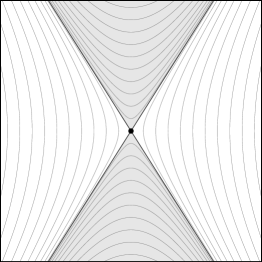
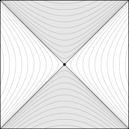
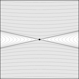
Figure 2: Level sets of different instances of $f_{a}$ for $a=(-4,1)$ (left), $a=(-1,1)$ (middle), and $a=(-1,20)$ (right), centered onto the saddle point. The scale of the axes is irrelevant since the problem is scale-invariant. The shaded areas correspond to positive function values. Problem difficulty increases from left to right, since the probability of sampling a “white” point (negative function value) in the vicinity of the saddle point shrinks.

For the two-dimensional case, three instances are plotted in Figure 2. The parameter $a$ controls the difficulty of the problem. The success probability of the (1+1)-ES at the saddle point $m=0$ equals $p_{\text{succ}}(0,\sigma)=\cot^{-1}(\sqrt{|a_{2}/a_{1}|})$, which decays to zero for $|a_{2}|\gg|a_{1}|$. This is a potentially fatal problem for the (1+1)-ES, since it may keep shrinking its step size and converge prematurely [5].

The contribution of this paper is to prove that we do not need to worry about this problem. More technically precise, we aim to establish the following theorem:

• Consider the sequence of states $(m_{t},\sigma_{t})_{t\in\mathbb{N}}$ of the (1+1)-ES on the function $f_{a}$. Then, with full probability, there exists $T\in\mathbb{N}$ such that for all $t\geq T$ it holds $f_{a}(m_{t})<0$.

It ensures that the (1+1)-ES surpasses the saddle point with full probability in finite time (iteration $T$). This implies in particular that the saddle point is not a limit point of the sequence $(m_{t})_{t\in\mathbb{N}}$ (see also Lemma 3 below).

3 Preliminaries

In this section, we prepare definitions and establish auxiliary results. We start by defining the following sets: $D_{a}^{-}=f_{a}^{-1}(\mathbb{R}_{<0})$, $D_{a}^{0}=f_{a}^{-1}(\{0\})$, and $D_{a}^{+}=f_{a}^{-1}(\mathbb{R}_{>0})$. They form a partition of the search space $\mathbb{R}^{d}$.

For a vector $x\in\mathbb{R}^{d}$ we define the semi-norms

$$\|x\|_{-}=\sqrt{-\sum_{i=1}^{b}a_{i}x_{i}^{2}}\qquad\text{and}\qquad\|x\|_{+}=\sqrt{\sum_{i=b+1}^{d}a_{i}x_{i}^{2}}\,.$$

The two semi-norms are Mahalanobis norms in the subspaces spanned by eigenvectors with negative and positive eigenvalues of the Hessian of $f_{a}$, respectively, when interpreting the Hessian with negative eigenvalues flipped to positive as an inverse covariance matrix. In other words, $f_{a}(x)=\|x\|_{+}^{2}-\|x\|_{-}^{2}$ holds. Furthermore, we have $\|x_{+}\|_{+}=\|x\|_{+}$, $\|x_{-}\|_{-}=\|x\|_{-}$, $\|x_{-}\|_{+}=0$, and $\|x_{+}\|_{-}=0$.

In the following, we exploit scale invariance of $f_{a}$ by analyzing the stochastic process $(m_{t},\sigma_{t})$ in a normalized state space. We map a state to the corresponding normalized state by

$$(m,\sigma)\mapsto\left(\frac{m}{\|m\|_{+}},\frac{\sigma}{\|m\|_{+}}\right)=(\tilde{m},\tilde{\sigma})\,.$$

This normalization is different from the normalizations $m/\sigma$ and $m/(d\sigma)$, which give rise to a scale-invariant process when minimizing the Sphere function [2]. The different normalization reflects the quite different dynamics of the (1+1)-ES on $f_{a}$.

We are particularly interested in the case $m\in D_{a}^{+}$, since we need to exclude the case that the (1+1)-ES stays in that set indefinitely. Due to scale invariance, this condition is equivalent to $\tilde{m}\in D_{a}^{+}$. We define the set

$$M=\big{\{}x\in\mathbb{R}^{d}\,\big{|}\,\|x\|_{+}=1\big{\}}\,.$$

The state space for the normalized states $(\tilde{m},\tilde{\sigma})$ takes the form $M\times\mathbb{R}_{>0}$. We also define the subset $M^{+}_{0}=M\cap(D_{a}^{+}\cup D_{a}^{0})$. The reason to include the zero level set is that closing the set makes it compact. Its boundedness can be seen from the reformulation $M^{+}_{0}=\big{\{}m\in\mathbb{R}^{d}\,\big{|}\,\|m\|_{+}=1\text{ and }\|m\|_{-}\leq 1\big{\}}$. In the following, compactness will turn out to be very useful, exploiting the fact that on a compact set, every lower semi-continuous function attains its infimum.

The success probability $p_{\text{succ}}(m,\sigma)$ is scale invariant, and hence it is well-defined as a function of the normalized state $(\tilde{m},\tilde{\sigma})$. It is everywhere positive. Indeed, it is uniformly lower bounded by $p_{\min}=\min(p^{*},\frac{1}{2})>0$, where $p^{*}=p_{\text{succ}}(0,1)$ denotes the success probability in the saddle point (which is independent of the step size, and depends only on $a$). The following two lemmas deal with the success rate in more detail.

• If there exists $T\in\mathbb{N}$ such that $m_{T}\in D_{a}^{0}\cup D_{a}^{-}$ then with full probability, the saddle point $0\in\mathbb{R}^{d}$ of $f_{a}$ is not a limit point of the sequence $(m_{t})_{t\in\mathbb{N}}$.

• Due to elitism, the sequence $m_{t}$ can jump from $D_{a}^{+}$ to $D_{a}^{0}$ and then to $D_{a}^{-}$, but not the other way round. In case of $m_{T}\in D_{a}^{-}$ all function values for $t>T$ are uniformly bounded away from zero by $f(m_{t})\leq f(m_{T})<0$. Therefore $f(m_{t})$ cannot converge to zero, and $m_{t}$ cannot converge to the saddle point.

  Now consider the case $m_{T}\in D_{a}^{0}$. For all $m\in D_{a}^{0}$ and all $\sigma>0$, the probability of sampling an offspring in $D_{a}^{-}$ is positive, and it is lower bounded by $p_{\min}$, which is positive and independent of $\sigma$. Not sampling an offspring $m_{t}\in D_{a}^{-}$ for $n$ iterations in a row has a probability of at most $(1-p_{\min})^{n}$, which decays to zero exponentially quickly. Therefore, with full probability, we obtain $m_{t}\in D_{a}^{-}$ eventually.              

However, $p_{\min}$ being positive is not necessarily enough for the (1+1)-ES to escape the saddle point, since for $p_{\min}<1/5$ it may stay inside of $D_{a}^{+}$, keep shrinking its step size, and converge prematurely [5]. In fact, based on the choice of the parameter $a$ of $f_{a}$, $p_{\min}$ can be arbitrarily small. In the following lemma, we therefore prepare a drift argument, ensuring that the normalized step size remains in or at least always returns to a not too small value.

• There exists a constant $0<\tilde{\sigma}_{\text{40\%}}\leq\infty$ such that $p_{\text{succ}}(\tilde{m},\tilde{\sigma})\geq 2/5$ holds for all states fulfilling $\tilde{m}\in M^{+}_{0}$ and $\tilde{\sigma}\leq\tilde{\sigma}_{\text{40\%}}$.

• It follows immediately from the geometry of the level sets (see also Figure 2) that for each fixed $\tilde{m}\in M^{+}_{0}$ (actually for $m\not=0$), it holds

  $$\lim\limits_{\tilde{\sigma}\to 0}p_{\text{succ}}(\tilde{m},\tilde{\sigma})=\frac{1}{2}\qquad\text{and}\qquad\lim\limits_{\tilde{\sigma}\to\infty}p_{\text{succ}}(\tilde{m},\tilde{\sigma})=p^{*}\,.$$

  Noting that $p_{\text{succ}}(\tilde{m},\tilde{\sigma})$ is continuous between these extremes, we define a pointwise critical step size as

  $$\tilde{\sigma}_{\text{40\%}}(\tilde{m})=\arg\min_{\tilde{\sigma}>0}\big{\{}p_{\text{succ}}(\tilde{m},\tilde{\sigma})\leq 2/5\big{\}}\,.$$

  With the convention that $\arg\min$ over an empty set is $\infty$, this definition makes $\tilde{\sigma}_{\text{40\%}}:M^{+}_{0}\to\mathbb{R}\cup\{\infty\}$ a lower semi-continuous function. Due to compactness of $M^{+}_{0}$ it attains its minimum $\tilde{\sigma}_{\text{40\%}}>0$.              

4 Drift of the Normalized State

In this section we establish two drift arguments. They apply to the following drift potential functions:

$$V(\tilde{m},\tilde{\sigma}) =\log(\tilde{\sigma})$$

$$W(\tilde{m},\tilde{\sigma}) =\|\tilde{m}\|_{-}$$

$$\Phi(\tilde{m},\tilde{\sigma}) =\beta\cdot V(\tilde{m},\tilde{\sigma})+W(\tilde{m},\tilde{\sigma})$$

The potentials govern the dynamics of the step size $\tilde{\sigma}$, of the mean $\tilde{m}$, and of the combined process, namely the (1+1)-ES. The trade-off parameter $\beta>0$ will be determined later. Where necessary we extend the definitions to the original state by plugging in the normalization, e.g., resulting in $W(m,\sigma)=\frac{\|m\|_{-}}{\|m\|_{+}}$.

For a normalized state $(\tilde{m},\tilde{\sigma})$ let $(\tilde{m}^{\prime},\tilde{\sigma}^{\prime})$ denote the normalized successor state. We measure the drift of all three potentials as follows:

$$\Delta^{V}(\tilde{m},\tilde{\sigma}) =\mathbb{E}\big{[}V(\tilde{\sigma}^{\prime})-V(\tilde{\sigma})\big{]}$$

$$\Delta^{W}(\tilde{m},\tilde{\sigma}) =\mathbb{E}\big{[}\min\{W(\tilde{m}^{\prime})-W(\tilde{m}),1\}\big{]}$$

$$\Delta^{\Phi}(\tilde{m},\tilde{\sigma}) =\beta\cdot\Delta^{V}(\tilde{m},\tilde{\sigma})+\Delta^{W}(\tilde{m},\tilde{\sigma})$$

As soon as $W(\tilde{m})>1$, $\tilde{m}\in D_{a}^{-}$ holds and the (1+1)-ES has successfully passed the saddle point according to Lemma 3. Therefore we aim to show that the sequence $W(\tilde{m}_{t})$ keeps growing, and that is passes the threshold of one. To this end, we will lower bound the progress $\Delta^{W}$ of the truncated process.

Truncation of particularly large progress in the definition of $\Delta^{W}$, i.e., $W$-progress larger than one, serves the purely technical purpose of making drift theorems applicable. This sounds somewhat ironic, since a progress of more than one on $W$ immediately jumps into the set $D_{a}^{-}$ and hence passes the saddle. On the technical side, an upper bound on single steps is a convenient prerequisite. Its role is to avoid that the expected progress is achieved by very few large steps while most steps make no or very litte progress, which would make it impossible to bound the runtime based on expected progress. Less strict conditions allowing for rare large steps are possible [6, 8]. The technique of bounding the single-step progress instead of the domain of the stochastic process was introduced in [2].

The speed of the growth of $W$ turns out to depend on $\tilde{\sigma}$. In order to guarantee growth at a sufficient pace, we need to keep the normalized step size from decaying to zero too quickly. Indeed, we will show that the normalized step size drifts away from zero by analyzing the step-size progress $\Delta^{V}$.

The following two lemmas establish the drift of mean $\tilde{m}$ and step size $\tilde{\sigma}$.

• Assume $\tilde{m}\in M^{+}_{0}$. There exists a constant $B_{1}$ such that $\Delta^{V}(\tilde{m},\tilde{\sigma})\geq B_{1}$ holds. Furthermore, there exist constants $B_{2}>0$ and $\tilde{\sigma}^{*}\in(0,\tilde{\sigma}_{\text{40\%}}]$ such that for all $\tilde{\sigma}\leq\tilde{\sigma}^{*}$ it holds $\Delta^{V}(\tilde{m},\tilde{\sigma})\geq B_{2}$.

• Assume $\tilde{m}\in M^{+}_{0}$. The $W$-progress $\Delta^{W}(\tilde{m},\tilde{\sigma})$ is everywhere positive. Furthermore, for each $\tilde{\sigma}^{*}\in(0,\tilde{\sigma}_{\text{40\%}}]$ there exists a constant $C>0$ depending on $\tilde{\sigma}^{*}$ such that it holds $\Delta^{W}(\tilde{m},\tilde{\sigma})\geq C$ if $\tilde{\sigma}\geq\tilde{\sigma}^{*}$.

The proofs of these lemmas contain the main technical work.

• From the definition of $\tilde{\sigma}_{\text{40\%}}$, for $\tilde{\sigma}\leq\tilde{\sigma}_{\text{40\%}}$, we conclude that the probability of sampling a successful offspring is at least $2/5$. In case of an unsuccessful offspring, $\tilde{\sigma}$ shrinks by the factor $\alpha^{-1/4}$. For a successful offspring it is multiplied by $\alpha\cdot\frac{\|m\|_{+}}{\|m^{\prime}\|_{+}}$, where the factor $\alpha>1$ comes from step size adaptation, and the fraction is due to the definition of the normalized state.

  The dependency on $m$ and $m^{\prime}$ is inconvenient. However, for small step size $\tilde{\sigma}$ we have $\|m^{\prime}\|\approx\|m\|$, simply because modifying $m$ with a small step results in a similar offspring, which is then accepted as the new mean $m^{\prime}$. In the limit we have

  $$\lim_{\tilde{\sigma}\to 0}\mathbb{E}\left[\log\left(\frac{\|m\|_{+}}{\|m^{\prime}\|_{+}}\right)\right]=0\,.$$

  This allows us to apply the same technique as in the proof of Lemma 3. The function $(\tilde{m},\tilde{\sigma})\mapsto\mathbb{E}\left[\log\left(\frac{\|m\|_{+}}{\|m^{\prime}\|_{+}}\right)\right]$ is continuous. We define a pointwise lower bound through the lower semi-continuous function

  $$\tilde{m}\mapsto\arg\min_{0<\tilde{\sigma}\leq\tilde{\sigma}_{\text{40\%}}}\left\{\mathbb{E}\left[\log\left(\frac{\|m\|_{+}}{\|m^{\prime}\|_{+}}\right)\right]\leq\frac{1}{\sqrt{\alpha}}\right\}\,,$$

  where the $\arg\min$ over the empty set shall take the value $\sigma_{\text{40\%}}$. We define $\tilde{\sigma}^{*}$ as its infimum. It is attained, since $M^{+}_{0}$ is compact, and hence positive.

  For $\tilde{\sigma}\leq\tilde{\sigma}^{*}$ we obtain the following drift condition:

  $$\Delta^{V}(\tilde{m},\tilde{\sigma}) \geq\frac{2}{5}\cdot\left[\log(\alpha^{-\frac{1}{2}})+\log(\alpha)\right]-\left(1-\frac{2}{5}\right)\cdot\frac{1}{4}\cdot\log(\alpha)$$

  $$=\frac{1}{5}\cdot\log(\alpha)-\frac{3}{20}\cdot\log(\alpha)=\frac{1}{20}\cdot\log(\alpha)>0$$

  For $\tilde{\sigma}>\tilde{\sigma}^{*}$ we consider the worst case of a success rate of zero. Then we obtain

  $$\Delta^{V}(\tilde{m},\tilde{\sigma})\geq-\frac{1}{4}\cdot\log(\alpha)\,.$$

  Hence, the statement holds with $B_{1}=-\frac{1}{4}\cdot\log(\alpha)$ and $B_{2}=\frac{1}{20}\cdot\log(\alpha)$.              

• We start by showing that $\Delta^{W}$ is always positive. We decompose the domain of the sampling distribution (which is all of $\mathbb{R}^{d}$) into spheres of fixed radius $r=\|\tilde{m}^{\prime}-\tilde{m}\|$ and show that the property holds, conditioned to the success region within each sphere. Within each sphere, the distribution is uniform.

  

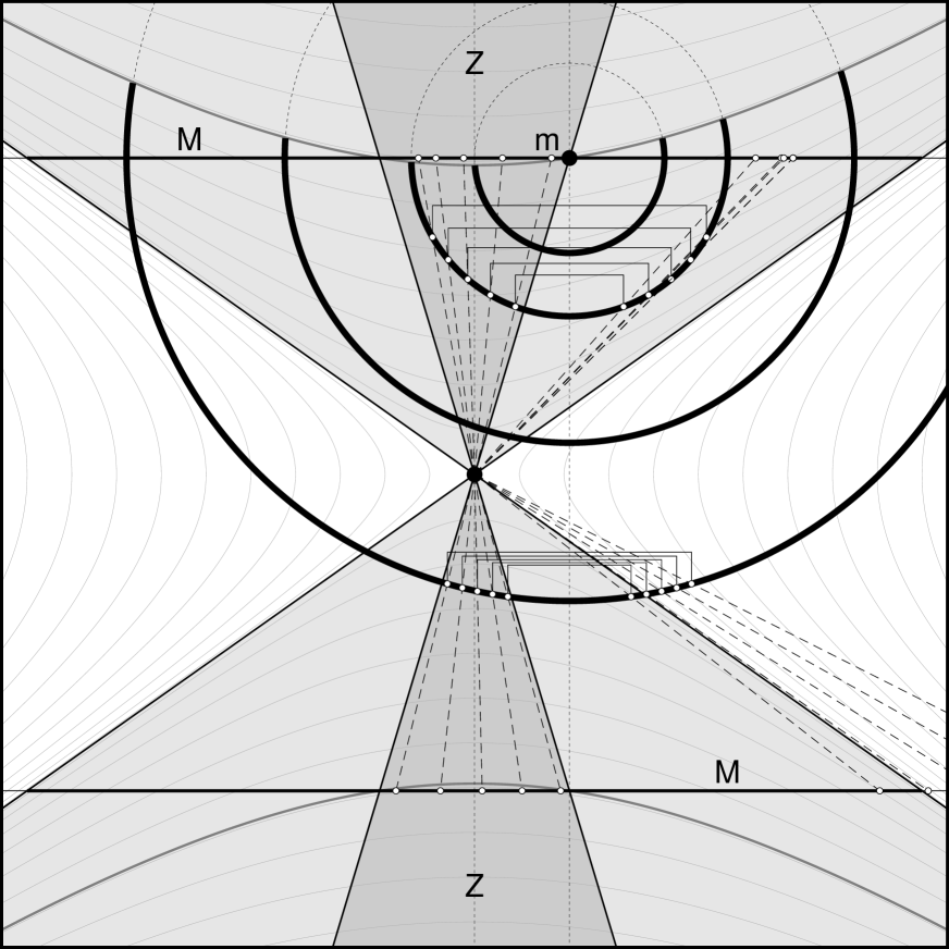
  Figure 3: Geometric illustration of the proof of Lemma 4. The figure shows the saddle point (center), level sets of $f_{a}$ (thin lines), the point $m$, and the set $M$ (two horizontal lines), the thick part of which is $M^{+}_{0}$. The area $D_{a}^{-}$ has a white background, while $D_{a}^{+}$ is the gray area. The dark gray area is the set $Z$.
  The figure displays spheres of different radii into which the sampling distribution is decomposed. The spheres are drawn as dotted circles, and as bold solid arcs in the region of successful offspring, outperforming $m$. The thickened arcs indicate sets of corresponding points. Ten pairs of corresponding points are shown, five each for two different spheres.

Each sphere makes positive and negative contributions to $W(x)-W(\tilde{m})=\frac{\|x\|_{-}}{\|x\|_{+}}-\|\tilde{m}\|_{-}$. Within the set

$$Z=\left\{z\in\mathbb{R}^{d}\,\left|\,\frac{\|z\|_{-}}{\|z\|_{+}}<\|\tilde{m}\|_{-}\right.\right\}$$

the contributions are negative. The set is illustrated in Figure 3. Outside of $Z$, contributions are positive. We aim to show that overall, for each sphere, the expectation is positive. To this end, we define pairs of corresponding points such that the negative contribution of one point is (more than) compensated by the positive contribution of the other. For our argument, it is important that the Lebesgue measure of each subset $S\subset Z$ is at most as large the Lebesgue measure of the set of corresponding points outside of $Z$. This property will be fulfilled by construction, and with equality.

For each successful offspring in $Z$ we define a corresponding point outside of $Z$ on the same sphere. Corresponding points are mirrored at the symmetry axis through $m$. More precisely, for $z\in Z$ we define $z^{\prime}_{-}=2m_{-}-z_{-}$ and $z^{\prime}_{+}=z_{+}$. It holds $\tilde{m}_{-}-z_{-}=z^{\prime}_{-}-\tilde{m}_{-}$, and we call this difference $\delta=\tilde{m}_{-}-z_{-}$.

By projecting both points onto the normalized state space $M$ we obtain their contributions to the expectation. This amounts to following the dashed lines in Figure 3. Adding the contributions of $z$ and $z^{\prime}$ yields

$$W(z)+W(z^{\prime})-2W(\tilde{m}) =\frac{\|z\|_{-}}{\|z\|_{+}}+\frac{\|z^{\prime}\|_{-}}{\|z^{\prime}\|_{+}}-2\|\tilde{m}\|_{-}$$

$$=\frac{\|\tilde{m}-\delta\|_{-}+\|\tilde{m}+\delta\|_{-}}{\|z\|_{+}}-2\|\tilde{m}\|_{-}$$

$$\geq\|\tilde{m}-\delta\|_{-}+\|\tilde{m}+\delta\|_{-}-2\|\tilde{m}\|_{-}\geq 0\,.$$

The first inequality holds because of $\|z\|_{+}=\|z^{\prime}\|_{+}\leq 1$ (note that the set $M$ corresponds to $\|\cdot\|_{+}=1$, see also Figure 3). The second step is the triangle inequality of the semi-norm $\|\cdot\|_{-}$. Both inequalities are strict outside of a set of measure zero.

Truncating progress $W(z^{\prime})-W(\tilde{m})$ larger than one does not pose a problem. This is because $W(\tilde{m})-W(z)<1$ is obtained from the fact that $\tilde{m}$ and $z$ are both contained in $D_{a}^{+}$, and this is where $W$ takes values in the range $[0,1)$. We obtain $W(z)-W(\tilde{m})+1>0$ in the truncated case.

Integrating the sum over all corresponding pairs on the sphere, and noting that there are successful points outside of $Z$ which do not have a successful corresponding point inside but not the other way round, we see that the expectation of $W(\tilde{m}^{\prime})-W(\tilde{m})$ over the success region of each sphere is positive.

Integration over all radii $r>0$ completes the construction. In the integration, the weights of different values of $r$ depend on $\tilde{\sigma}$ (by means of the pdf of a $\chi$-distribution scaled by $\tilde{\sigma}$). Since the integrand is non-negative, we conclude that $\Delta^{W}(\tilde{m},\tilde{\sigma})>0$ holds for all $\tilde{\sigma}>0$.

In the limit $\tilde{\sigma}\to\infty$, the expected progress in case of success converges to one (due to truncation), and hence the expected progress converges to $p^{*}$. This allows us to exploit compactness once more. The expectation of the truncated progress $\Delta^{W}(\tilde{m},\tilde{\sigma})$ is continuous as a function of the normalized state. We define a pointwise lower bound as

$$C(\tilde{m})=\min_{\tilde{\sigma}\geq\tilde{\sigma}_{\text{40\%}}}\Big{\{}\Delta^{W}(\tilde{m},\tilde{\sigma})\Big{\}}\,.$$

$C(\tilde{m})$ is a continuous function, and (under slight misuse of notation) we define $C$ as its infimum over the compact set $M^{+}_{0}$. Since the infimum is attained, it is positive.              

Now we are in the position to prove the theorem.

• Combining the statements of Lemma 4 and 4 we obtain

  $$\Delta^{\Phi}(\tilde{m},\tilde{\sigma})\geq\theta:=\min\{\beta B_{2},C+\beta B_{1}\}\,$$

  for all $\tilde{m}\in M^{+}_{0}$ and $\tilde{\sigma}>0$. The choice $\beta=\frac{-C}{2B_{1}}$ results in $\theta=\min\{B_{2},C/2\}>0$. The constant $\theta$ is a bound on the additive drift of $\Phi$, hence we can apply additive drift with tail bound (e.g., Theorem 2 in [8] with additive drift as a special case, or alternatively inequality (2.9) in Theorem 2.3 in [6]) to obtain the following: Let

  $$T=\min\Big{\{}t\in\mathbb{N}\,\Big{|}\,\Phi(\tilde{m}_{t},\tilde{\sigma}_{t})>1\Big{\}}$$

  denote the waiting time for the event that $\Phi$ reaches or exceeds one (called the first hitting time). Then the probability of $T$ exceeding $T_{0}\in\mathbb{N}$ decays exponentially in $T_{0}$. Therefore, with full probability, the hitting time $T$ is finite. $\Phi(\tilde{m}_{T},\tilde{\sigma}_{T})>1$ is equivalent to $f(m_{T})<0$. For all $t>T$, the function value stays negative, due to elitism.              

5 Discussion and Conclusion

We have established that the (1+1)-ES does not get stuck at a (quadratic) saddle point, irrespective of its conditioning (spectrum of its Hessian), with full probability. This is all but a trivial result since the algorithm is suspectable to premature convergence if the success rate is smaller than $1/5$. For badly conditioned problems, close to the saddle point, the success rate can indeed be arbitrarily low. Yet, the algorithm passes the saddle point by avoiding it “sideways”: While approaching the level set containing the saddle point, there is a systematic sidewards drift away from the saddle. This keeps the step size from decaying to zero, and the saddle is circumvented.

In this work we are only concerned with quadratic functions. Realistic objective functions to be tackled by evolution strategies are hardly ever so simple. Yet, we believe that our analysis is of quite general value. The reason is that the negative case, namely premature convergence to a saddle point, is an inherently local process, which is dominated by a local approximation like the second order Taylor polynomial around the saddle point. Our analysis makes clear that as long as the saddle is well described by a second order Taylor approximation with a full-rank Hessian matrix, then the (1+1)-ES will not converge prematurely to the saddle point. We believe that our result covers the most common types of saddle points. Notable exceptions are sharp ridges, plateaus, and Monkey saddles.

The main limitation of this work is not the covered class of functions, but the covered algorithms. The analysis sticks closely to the (1+1)-ES with its success-bases step size adaptation mechanism. There is no reason to believe that a fully fledged algorithm like the covariance matrix adaptation evolution strategy (CMA-ES) [hansen:2001] would face more problems with a saddle than the simple (1+1)-ES, and to the best of our knowledge, there is no empirical indication thereof. In fact, our intuition is that most algorithms should profit from the sidewards drift, as long as they manage to break the symmetry of the problem, e.g., through randomized sampling. Yet, it should be noted that our analysis does not easily extend to non-elitist algorithms and step size adaptation methods other than success-based rules.

References

- [1] Youhei Akimoto. Saddle point optimization with approximate minimization oracle. Technical Report 2103.15985, arXiv.org, 2021.
- [2] Youhei Akimoto, Anne Auger, and Tobias Glasmachers. Drift theory in continuous search spaces: Expected hitting time of the (1+1)-es with 1/5 success rule. In Proceedings of the Genetic and Evolutionary Computation Conference (GECCO). ACM, 2018.
- [3] Youhei Akimoto, Yuichi Nagata, Isao Ono, and Shigenobu Kobayashi. Theoretical analysis of evolutionary computation on continuously differentiable functions. In Genetic and Evolutionary Computation Conference, pages 1401–1408. ACM, 2010.
- [4] Yann N Dauphin, Razvan Pascanu, Caglar Gulcehre, Kyunghyun Cho, Surya Ganguli, and Yoshua Bengio. Identifying and attacking the saddle point problem in high-dimensional non-convex optimization. In Z. Ghahramani, M. Welling, C. Cortes, N. D. Lawrence, and K. Q. Weinberger, editors, Advances in Neural Information Processing Systems 27, pages 2933–2941. 2014.
- [5] Tobias Glasmachers. Global convergence of the (1+1) evolution strategy. Evolutionary Computation Journal (ECJ), 28(1):27–53, 2020.
- [6] Bruce Hajek. Hitting-time and occupation-time bounds implied by drift analysis with applications. Advances in Applied probability, pages 502–525, 1982.
- [7] S. Kern, S. D. Müller, N. Hansen, D. Büche, J. Ocenasek, and P. Koumoutsakos. Learning probability distributions in continuous evolutionary algorithms–a comparative review. Natural Computing, 3(1):77–112, 2004.
- [8] Per Kristian Lehre and Carsten Witt. General drift analysis with tail bounds. Technical Report 1307.2559, arXiv.org, 2013.