First Steps of an Approach to the ARC Challenge based on Descriptive Grid Models and the Minimum Description Length Principle

Abstract

The Abstraction and Reasoning Corpus (ARC) was recently introduced by François Chollet as a tool to measure broad intelligence in both humans and machines. It is very challenging, and the best approach in a Kaggle competition could only solve 20% of the tasks, relying on brute-force search for chains of hand-crafted transformations. In this paper, we present the first steps exploring an approach based on descriptive grid models and the Minimum Description Length (MDL) principle. The grid models describe the contents of a grid, and support both parsing grids and generating grids. The MDL principle is used to guide the search for good models, i.e. models that compress the grids the most. We report on our progress over a year, improving on the general approach and the models. Out of the 400 training tasks, our performance increased from 5 to 29 solved tasks, only using 30s computation time per task. Our approach not only predicts the output grids, but also outputs an intelligible model and explanations for how the model was incrementally built.

1 Introduction

This document describes our approach to the ARC (Abstraction and Reasoning Corpus) challenge introduced by François Chollet as a tool to measure intelligence, both human and artificial [2]. ARC was introduced in order to foster research on Artificial General Intelligence (AGI) [5], and to move from system-centric generalization to developer-aware generalization. The latter enables a system to “handle situations that neither the system nor the developer of the system have encountered before”. For instance, a system trained to recognize cats features system-centric generalization because it can recognize cats that it has never seen, but in general, it does not feature developer-aware generalization because it can not learn to recognize horses with only a few examples (unlike a young child would).

ARC is made of 1000 learning tasks, 400 for training, 400 for evaluation, and 200 kept secret by its author in order to ensure bias-free evaluation. Each task consists in learning how to generate an output colored grid from an input colored grid (see Figure 1 for an example). ARC is a challenging target for AI. As F. Chollet writes: “to the best of our knowledge, ARC does not appear to be approachable by any existing machine learning technique (including Deep Learning)” [2]. The main difficulties are the following:

• The expected output is not a label, or even a set of labels, but a colored grid with size up to 30x30, and with up to 10 different colors. It therefore falls in the domain of structured prediction [3].

• The predicted output has to match exactly the expected output. If a single cell is wrong, the task is considered as failed. To compensate for that, three attempts are allowed for each input grid.

• In each task, there are generally between 2 and 4 training instances (input grid + output grid), and 1 or 2 test instances for which a prediction has to be made.

• Each task relies on a distinct transformation from the input grid to the output grid. In particular, no evaluation task can be solved by reusing a transformation learned on the training tasks. Actually, each task is a distinct learning problem, and what ARC evaluates is broad generalization and few-shot learning.

A compensation for those difficulties is that the the input and output data are much simpler than real-life data like photos or texts. We think that this helps to focus on the core features of intelligence rather than on scalability issues.

A kaggle competition was organized in Spring 2020 to challenge the robustness of ARC as a measure of intelligence, and to see what could be achieved with state-of-the-art techniques. The winner’s solution manages to solve 20% over 100 (secret) evaluation tasks, which is already a remarkable performance. However, it is based on the brute-force search for chains of grid transformations, chosen from a hand-crafted set of 142 elementary transformations. This can hardly scale to larger sets of tasks, and as the author admits: “Unfortunately, I don’t feel like my solution itself brings us closer to AGI.” Another competitor used a similar domain-specific language based on transformations, and grammatical evolution to search the program space [4]. Their approach solves 3% of the Kaggle tasks, and 7.68% over the 400 training tasks.

Our approach is based on the MDL (Minimum Description Length) principle [9, 6] according to which “the best model for some data is the one that compresses the most the data”. The MDL principle has already been applied successfully to pattern mining of various data structures (transactions [11], sequences [10], relational databases [7], or graphs [1]), as well as classification [8]. A major difference with those work is that the model to be learned needs not only explain the data but also be able to perform a structured prediction, here the output grid from the input grid. At this stage (Version 2.2), we consider rather simple models that have no chance to cover a large proportion of ARC tasks: single-color points and shapes, and basic arithmetic of positions and sizes. Our prime objective is to demonstrate the effectiveness of an MDL-based approach to the ARC challenge, and hopefully to AGI. Our approach succeeds on 29/400 (7.25%) training tasks and 6/400 (1.5%) evaluation tasks, with a learning timeout of 30s only per task. We find such a result quite encouraging given the difficulty of the problem. Moreover, the solved tasks are quite diverse, and the learned model is often close to the simplest model for the task (in the chosen class of models).

This report is organized as follows. Section 2 gives a formal definition of ARC grids and tasks. Section 3 explains our modelling of the ARC tasks in the framework of two-parts MDL, in particular our class of models. Section 4 describes the MDL-based learning process, which boils down to defining description lengths and model refinements. Section 5 reports on the evaluation of our approch on training and evaluation ARC tasks, as well as on the learned models for a few tasks.

2 Defining ARC Tasks

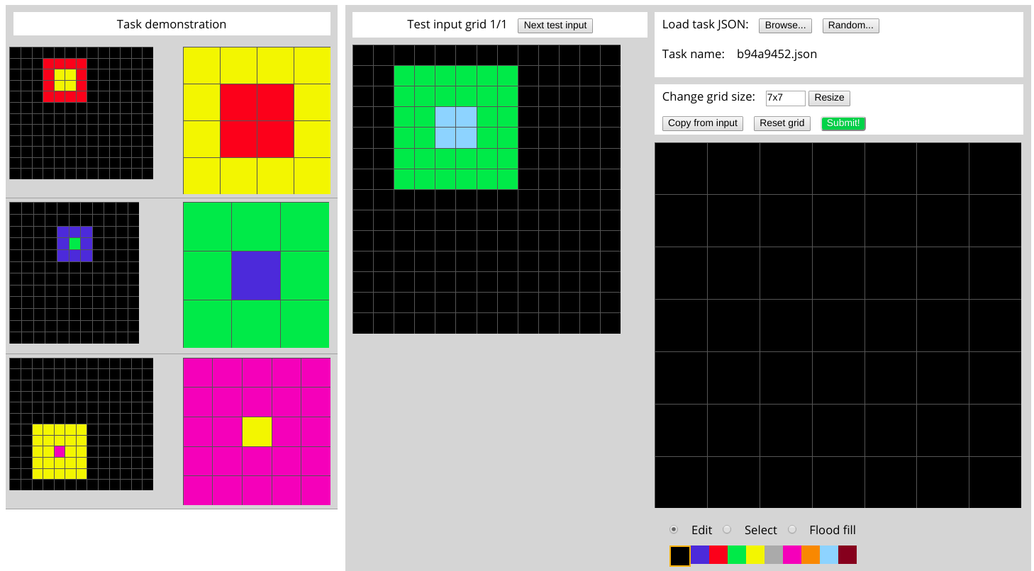
Figure 1: One of the training tasks (b94a9452), with three examples on the left, a test input grid in the middle, and the widget on the right that can be used to draw the missing output grid.

Definition 1 (colors)

We assume a finite set $C$ of distinct symbols, which we call colors.

In ARC, there are 10 colors coded by digits (0..9) in JSON files, and by colors (e.g., black, purple, red) in the web interface (see Figure 1).

Definition 2 (grid)

A grid $g\in C^{h\times w}$ is a matrix of colors with $h>0$ rows, and $w>0$ columns. A grid is often displayed as a colored grid. The number of rows $h={\it height}(g)$ is called the height of the grid, and the number of columns $w={\it width}(g)$ is called the width of the grid.

A grid cell is caracterized by coordinates $(i,j)$, where $i$ selects a row, and $j$ selects a column. The color at coordinates $(i,j)$ is denoted either by $g_{ij}$ or by $g[i,j]$. Coordinates range from $(0,0)$ to $(h-1,w-1)$.

In ARC, grids have a size from $1\times 1$ to $30\times 30$.

Definition 3 (example)

An example is a pair of grids $e=(g^{i},g^{o})$, where $g^{i}$ is called the input grid, and $g^{o}$ is called the output grid.

As illustrated by Figure 1, the output grid needs not have the same size as the input grid, it can be smaller or bigger.

Definition 4 (task)

A task is a pair $T=(E,F)$, where $E$ is the set of train examples, and $F$ is the set of test examples.

The learner has only access to the input and ouput grids of the train examples. Its objective is, for each test example, to predict the output grid given the input grid. As illustrated by Figure 1, the different input grids of a task need not have the same size, nor use the same colors. The same applies to test grids.

The ARC is composed of 1000 tasks in total: 400 for training, 400 for evaluation by developers, and 200 for independent evaluation. Figure 1 shows one of the 400 training tasks, with three train examples, and one test input grid. Developers should only look at the training tasks, not at the evaluation tasks, which should only be used to evaluate the broad generalization capability of the system. Each task has generally between 2 and 4 train examples, and 1 or 2 test examples.

3 Modelling ARC Tasks in Two-Parts MDL

The objective is here to design a class of task models that can be used to represent a transformation from input grids to output grids. Our key intuition is that a task model can be decomposed into two grid models, one for the input grids, and another for the output grids. The input grid model expresses what all train input grids have in common, while the output grid model expresses what all train output grids have in common, as a function of the input grid. The actual transformation from input grid to output grid involves the two models as follows. The input grid model is used to parse the input grid, which produces some information that characterizes the input grid. Then, that parsing information is fed into the output grid model in order to generate an output grid.

In the following, paragraphs starting with Version X are specific to that version, in contrast to other paragraphs that are generic.

3.1 Models

$\begin{array}[]{lcl}{\it Pair}&\ ::=&{\bf InOut}(in:{\it Grid},out:{\it Grid})\\ {\it Grid}&\ ::=&{\bf Grid}(size:{\it Vector},\ color:C,\ layers:list({\it Object}))\\ {\it Object}&\ ::=&{\bf PosShape}(pos:{\it Vector},\ shape:{\it Shape})\\ {\it Shape}&\ ::=&{\bf Point}(color:C)\\ &\ \mid&{\bf Rectangle}(size:{\it Vector},\ color:C,\ mask:{\it Mask})\\ {\it Vector}&\ ::=&{\bf Vec}(i:\mathbb{N},\ j:\mathbb{N})\\ {\it Mask}&\ ::=&{\bf Bitmap}(bitmap:M)\\ &\ \mid&{\bf Full}\ \mid\ {\bf Border}\\ &\ \mid&{\bf EvenCheckboard}\ \mid\ {\bf OddCheckboard}\\ &\ \mid&{\bf PlusCross}\ \mid\ {\bf TimesCross}\end{array}$

Figure 2: Datatypes used in grid models and grid data

Version 2.

The main component of our grid models is objects. Indeed, ARC grids can often be read as objects with various shapes over a background. Objects can be disconnected, nested or overlap each other. Each object has a position and a shape.

A shape has a color, and either it is a point, or it fits into a rectangular box of some size. In the latter case, the precise shape is specified by a mask that can be a custom bitmap or one of a few pre-defined regular shapes. The position of objects is relative to the top-left cell of the shape. Each object attribute (e.g., position, size, color) may be constant (e.g., the shape is always red) or variable across the examples.

We define our models as templates over data structures representing concrete pairs of grids. Figure 2 defines those data structure with algebraic data types for gird pairs, grids, objects, shapes, masks, and vectors (2D positions and sizes). They use primitive types for natural numbers ($\mathbb{N}$), colors ($C$), and 2D bitmaps (${\it M}$). Uppercase names in bold are called constructors, and the lowercase names of constructor arguments are called fields.

A task is made of two grids, one for the input grid, and another for the output grid. Each grid is described as a stack of layers on top of a background, each layer being made of a single object. The background has a size (a 2D vector), and a color. An object is a shape at some position. A shape is either a point, described by its color; or a rectangle, described by its size, color, and mask. That mask allows to account for regular and irregular shapes, and indicates which pixels in the rectangle box actually belong to the shape (other pixels can be seen as transparent). A mask can be a custom bitmap or one of a few common regular shapes: full rectangle, rectangle border, checkboards, and centered crosses. A data structure describing the first train pair in Figure 1 is:

$$\begin{array}[]{l}{\bf InOut}(\\ \quad{\bf Grid}({\bf Vec}(12,13),black,\\ \quad\quad[{\bf PosShape}({\bf Vec}(2,4),{\bf Rectangle}({\bf Vec}(2,2),yellow,{\bf Full})),\\ \quad\quad\leavevmode\nobreak\ {\bf PosShape}({\bf Vec}(1,3),{\bf Rectangle}({\bf Vec}(4,4),red,{\bf Full})])),\\ \quad{\bf Grid}({\bf Vec}(4,4),yellow,\\ \quad\quad[{\bf PosShape}({\bf Vec}(1,1),{\bf Rectangle}({\bf Vec}(2,2),red,{\bf Full})]))).\end{array}$$

A path in a data structure is a sequence of fields that goes from the root of the data structure to some sub-structure. In the above example, path $in.size.j$ refers to the input grid width, which is $13$; path $out.layers[0].shape.color$ refers to the color of the top shape in the output grid. which is $red$; and path $in.layers[1].pos$ refers to the position of the bottom shape in the input grid, which is ${\bf Vec}(1,3)$. Given a data structure $d$ and a path $p$, the substructure of $d$ that is refered by $p$ is written with the dot-notation $d.p$.

In order to generalize from specific pairs of grids to general task models, we introduce two kinds of elements that can be used in place of any sub-structure: unknowns and expressions. An unknown, which we note with a question mark $?$, indicates that any data structure of the expected type can fit in. For example, a grid model that matches all input grids in Figure 1 is:

$$\begin{array}[]{l}{\bf Grid}({\bf Vec}(12,?),black,\\ \quad[{\bf PosShape}(?,{\bf Rectangle}(?,?,?)),\\ \quad\leavevmode\nobreak\ {\bf PosShape}(?,{\bf Rectangle}(?,?,{\bf Full}))])\end{array}$$

It matches grids with 12 rows and a black background, and two stacked rectangles of any position, any size, and any color. The top rectangle may have any mask, while the bottom rectangle should be full. The purpose of parsing is to fill in the holes, replacing unknowns with data structures such that the whole resulting data structure correctly describes a grid or a pair of grids. An unknown path is a path in the model that leads to an unknown. The unknown paths in the above grid model are: $size$, $layers[0].pos$, $layers[0].shape.size$, $layers[0].shape.color$, $layers[0].shape.mask$, $layers[1].pos$, $layers[1].shape.size$, $layers[1].shape.color$. The set of unknown paths of a model $m$ is denoted by $U(m)$.

A data structure that may contain unknowns is called a pattern. A data structure is said ground if it contains no unknown. Given a ground data structure $d$ and a pattern $p$, the notation $d\sim p$ says that $d$ agrees with $p$ or that $p$ matches $d$. It means that the ground data structure $d$ can be obtained by a substitution of the pattern unknowns with ground data structures. For example, we have ${\bf Vec}(12,14)\sim{\bf Vec}(12,?)$.

An expression defines part of the data structure as the result of a computation over some input data structure, which we call the environment. Expressions are made of primitive values, constructors, operators/functions, and variables. In Version 2, the only operators are zero, addition and substraction over natural numbers, they are used to compute the position and size of grids and shapes. Variables are references to parts of the environment. A convenient way to refer to such parts is to use paths in the environment data structure. Expressions that would only be made of primitive values and constructors would actually be data structures, and are therefore not considered as expressions. The environment of the output grid is the input grid, so that parts of the output grid can be computed based on the input grid contents. The input grid has no environment so that expressions are not useful in the input grid model. Re-using the above model for input grids, we can now define a correct and complete model for the task in Figure 1, using unknowns for the input grid, and expressions for the output grid:

$$\begin{array}[]{l}{\bf InOut}(\\ \quad{\bf Grid}({\bf Vec}(12,?),black,\\ \quad\quad[\leavevmode\nobreak\ {\bf PosShape}({\bf Vec}(?,?),{\bf Rectangle}({\bf Vec}(?,?),?,{\bf Full})),\\ \quad\quad\leavevmode\nobreak\ \leavevmode\nobreak\ {\bf PosShape}({\bf Vec}(?,?),{\bf Rectangle}({\bf Vec}(?,?),?,{\bf Full})\leavevmode\nobreak\ ])),\\ \quad{\bf Grid}(layers[1].shape.size,layers[0].shape.color,\\ \quad\quad[\leavevmode\nobreak\ {\bf PosShape}(\\ \quad\quad\quad\quad{\bf Vec}(layers[0].pos.i-layers[1].pos.i,\ layers[0].pos.j-layers[1].pos.j),\\ \quad\quad\quad\quad{\bf Rectangle}(layers[0].size,\ layers[1].color,\ {\bf Full}))\leavevmode\nobreak\ ])).\end{array}$$

In words, this models says: “find two stacked full rectangles on a black background in the input grid, then generate an output grid, whose size is the same as the bottom shape, and whose background color is the color of the top shape, and finally add a full rectangle whose size is the same as the top shape, whose color is the same as the bottom shape, and whose position is the difference between the top shape position and the bottom shape position (relative position).”

A model is well-formed if it is well-typed (constructor arguments, operator operand types, etc.), and if all variables are valid paths in the environment data. More specifically, a task model is well-formed if the input grid model contains no variable, and if all variables in the output grid model are valid paths in the input grid model.

A task model is definite if its output grid model contains no unknown, so that it can be used to deterministically generate an output grid from a data structure describing the input grid.

3.2 Data According to a Model

In MDL-based approaches, it is essential to have a lossless encoding of data in order to have a fair comparison of different models. Therefore, it is important to identify the “data according to the model”, i.e. the data that needs to be added to a model in order to capture all the information in the original data.

We first consider grid models, where data is a grid. An analogy can be made with formal languages and grammars. In this analogy, grids are sentences, grid models are grammars, and data according to the model is the parse tree. A parse tree explains how the grammar generates the sentence. Here, data structures as defined in Figure 2 play the role of parse trees for grid models, they are grid parse trees and we denote them with the greek letter $\pi$. A grid parse tree, the data according to the model, is a data structure that instantiates the grid model by replacing expressions by their value, and unknowns by values such that the resulting data structure correctly describes the grid. The description length will only count the data structures that instantiate the unknowns because the rest of the parse tree is already known from the model.

For input grid $g^{i}_{k}$ ($k$-th example), $\pi^{i}_{k}$ denotes one possible grid parse tree according to some fixed input grid model $m^{i}$. Similarly, for output grid $g^{o}_{k}$, $\pi^{o}_{k}$ denotes one possible grid parse tree according to some fixed output grid model $m^{o}$ and output environment $\varepsilon^{o}$.

In practice, a grid model may not explain all the cells of a grid. This happens in case of noise in the data, and also in the learning process where intermediate models are obviously incomplete. To account for those situations without losing information, we define “data according to the model” as a grid parse tree plus the list of cells that differ between the original grid $g$ and the grid generated by the grid parse tree $\pi$. We call this additional information a grid delta, written $\delta$.

An additional difficulty is when a test input grid does not match the input grid model learned from the train examples. For instance, all input grids in the train examples have size (10,10) but the test input grid has size (10,12). In this case, there is no grid parse tree that agrees with both the grid model and the grid. In many cases, this discrepancy does not alter the validity of the model, which only happens to be overspecific (a form of overfitting). Our approach to this difficulty is to allow for approximate parsing, i.e. to allow grid parse trees to diverge from the grid model. As those differences are present in the grid parse tree $\pi$, there is no loss of information. Of course, the description length will take into acount such differences to penalize them.

As an illustration, let us consider the following (incomplete) input grid model for the task in Figure 1:

$${\bf Grid}(?,black,[\ {\bf PosShape}(?,{\bf Rectangle}(?,?,{\bf Full}))\ ]).$$

There are mainly two “data according to the model” for the first input grid $g^{i}_{1}$ (the upper index is $i$ for input grids and $o$ for output grids, the lower index identifies the example):

1. matching the outer red rectangle
   $\pi^{i}_{1}={\bf Grid}({\bf Vec}(12,13),black,$
                     $[\ {\bf PosShape}({\bf Vec}(1,3),{\bf Rectangle}({\bf Vec}(4,4),red,{\bf Full}))\ ])$
   $\delta^{i}_{1}=\{(2,4,yellow),(2,5,yellow),(3,4,yellow),(3,5,yellow)\}$

2. matching the inner yellow rectangle
   $\pi^{i}_{1}={\bf Grid}({\bf Vec}(12,13),black,$
                     $[\ {\bf PosShape}({\bf Vec}(2,4),{\bf Rectangle}({\bf Vec}(2,2),yellow,{\bf Full}))\ ])$
   $\delta^{i}_{1}=\{(1,3,red),(1,4,red),(1,5,red),(1,6,red),(2,3,red),(2,6,red),(3,3,red),...\}$

The first solution looks better because it has a much smaller grid delta, and its grid parse tree has the same size as in the second solution.

3.3 Primitive Functions on Grids, Grid Models, Grid Parse Trees, and Grid Deltas

We here define the key primitive functions to manipulate grids, grid models, grid parse trees and grid deltas.

We first define grid deltas and simple arithmetics on them.

Definition 5 (grid delta)

Let $g_{1},g_{2}\in C^{h\times w}$ two same-size grids. The grid delta $\delta\subseteq\mathbb{N}\times\mathbb{N}\times C$ between the two grids, written $g_{2}-g_{1}$, is defined as the set of cells that need changing color in $g_{1}$ in order to obtain $g_{2}$.

$$\delta=g_{2}-g_{1}=\{(i,j,c)\mid g_{2}[i,j]\neq g_{1}[i,j],c=g_{2}[i,j]\}$$

A grid delta $\delta$ can be added to a grid $g_{1}$ to get a corrected same-size grid $g_{2}$.

$$g_{2}=g_{1}+\delta\iff\forall i\in[0,h[,j\in[0,w[:g_{2}[i,j]=\left\{\begin{array}[]{ll}c&\quad\textrm{if\leavevmode\nobreak\ }(i,j,c)\in\delta\\ g_{1}[i,j]&\quad\textrm{otherwise}\\ \end{array}\right.$$

Then we define two functions that are directly related to the semantics of grid models. The first function converts a grid parse tree into a grid.

Definition 6 (grid drawing)

Let $\pi$ be a grid parse tree, ${\it draw}(\pi)$ is the grid that results from the drawing following the instructions given by the grid parse tree.

Version 2.

Given a grid parse tree $\pi$ as specified in Figure 2, the grid ${\it draw}(\pi)$ is obtained by first generating a grid with the specified size and background color, and then layers are drawn on that grid, bottom-up. Each layer, either a point or a rectangle, is drawn in the obvious way. For a point ${\bf PosShape}({\bf Vec}(i,j),{\bf Point}(c))$, the cell at position $(i,j)$ is set to color $c$. For a rectangle ${\bf PosShape}({\bf Vec}(i,j),{\bf Rectangle}({\bf Vec}(h,w),c,m))$, each cell at position $(i+x,j+y)$, for any $x\in[0,h[$ and $y\in[0,w[$, is set to color $c$ if the relative position $(x,y)$ belongs to mask $m$.

The second function applies a grid model to an environment, resolving references to it, and replacing expressions by their evaluation result.

Definition 7 (model application)

Let $m$ be a grid model, and $\varepsilon$ an environment for the model. ${\it apply}(m,\varepsilon)$ is the model that results from the substitution of expressions in $m$ by their evaluation over the environment $\varepsilon$. The resulting model has no expression but may still have unknowns. The operation is ill-defined if some variable in $m$ is not defined in $\varepsilon$.

Version 2.

Environments are grid parse trees, and variables are paths into them. There are only three operators – zero, plus, minus – and they are evaluated in the usual way on integer values.

We also define two non-deterministic functions that produce grid parse trees from a grid model, and hence grid descriptions. The first function corresponds to the parsing of a grid.

Definition 8 (grid parsing)

Let $m$ be a grid model, and $g$ be a grid. ${\it parse}(m,g)$ non-deterministically returns a grid parse tree $\pi$ that approximately agrees with model $m$, and approximately draws as grid $g$. Non-determinism allows for different interpretations of the grid by the model.

Version 2.

This is by far the most complex primitive function. Parsing is decomposed in three stages. First, the grid is partitioned into contiguous monocolor regions. Second, objects are looked for as single parts or as unions of parts to cover the case where some objects are overlaped by other objects. Small parts (less than 5 covered cells) are also considered as adjacent individual points. When an object’s shape is not a point or a full rectangle, two shapes are considered: one shape with a full mask, considering the missing cells as noise on top of the rectangle; and another shape with a mask containing the cells in the rectangle box that belong to the object and have the same color. A regular mask is used when possible (e.g., borders, crosses), otherwise a bitmap is used. Third, matching superpositions of objects are looked for according to the grid model. For each layer, candidate objects are considered in a fixed ordering that includes some simple heuristics. Black objects are considered last because black is often the background color. Then, objects are considered in decreasing number of covered cells. Beyond those heuristics, a total ordering is defined because it makes experiments more reproducible, and also because it helps disambiguate some situations. For instance, if the model contains several points, they will be matched to points in the grid from left to right, top-down. Layers are parsed top-down. When done in a naive recursive way, the search space is not be explored in fair way. Indeed, the second candidate object for the frst layer is only considered when all candidates have been considered for the other layers in combination with the first candidate object for the first layer. Defining the rank of a parse tree for all layers as the sum of the rank of the chosen candidate object of each layer, we explore the search space in increasing rank to favor the first candidate objects across all layers. This improvement was introduced in Version 2.2.

As an example of parsing, the test input grid in Figure 1 has three contiguous parts: the light blue one, the green one, and the black one. Three rectangles can be identified from those parts: a small light blue square, a green rectangle overlaped by the blue one, and a black rectangle covering the whole grid and overlaped by the other rectangles. According to the above model, this input grid is parsed as a 2x2 light blue rectangle at coordinates (3,4), on top of a 6x6 green rectangle at coordinates (1,2), on top of a black background.

Compared to Version 1, parsing has been made non-deterministic in the sense that a sequence of grid parse trees is produced. We use the description lengths as defined below to order this sequence from the shorter DL to the longer DL. Indeed, the shorter the DL, the more plausible the grid parse tree is. Because of combinatorial problems in the parsing process, we use various bounds: maximum number of candidate objects for a given layer in the model, maximum number of produced grid parse trees before sorting them, and maximum number of grid parse trees actually returned. Relative to approximate parsing, we also bound the number of differences w.r.t. the model.

The second function corresponds to generation, where the grid parse tree is produced by filling in the holes of the grid model, i.e. guessing at the missing elements.

Definition 9 (grid generation)

Let $m$ be a grid model without any expression. ${\it generate}(m)$ non-deterministically returns a grid parse tree that is obtained by replacing unknowns in the model by type-compatible sub-trees.

Version 2.

We simply replace unknowns by default values. It makes it very unlikely to generate the right output grid by chance but it helps to visualize the intermediate states of the learning process. The default position is $(0,0)$, the default size is $(10,10)$ for grids, and $(2,2)$ for rectangles, the default color is black for grids and grey for shapes, the default mask is the full mask, the default shape is a rectangle with default values in each field.

3.4 Reading and Writing a Grid with a Grid Model

We define two important components for reading and writing grids. They are simply composed from the above primitve functions, and are used as basic blocks for training and using models.

Figure 3: The read component.

Figure 4: The write component.

Definition 10 (grid reading)

Let $m$ be a model. Function ${\it read}_{m}$ takes an environment and a grid as input, and returns a grid parse tree and delta as output.

$${\it read}_{m}(\varepsilon,g)=\{(\pi,\delta)\mid m_{\varepsilon}={\it apply}(m,\varepsilon),\pi\in{\it parse}(m_{\varepsilon},g),\delta=g-{\it draw}(\pi)\}$$

Figure 4 gives a schematic description of the read component. When reading a grid $g$, the grid model is first applied to the input environment, in order to resolve any expression that the model may contain. The resulting model is then used to parse the input grid into a grid parse tree $\pi$. Finally, the grid delta between the grid specified by $\pi$ and $g$ is computed. The pair $(\pi,\delta)$ provides a lossless representation of the input grid, as expressed by the following lemma.

$$(\pi,\delta)\in{\it read}_{m}(\varepsilon,g)\Longrightarrow g={\it draw}(\pi)+\delta.$$

Definition 11 (grid writing)

Let $m$ be a grid model. Function ${\it write}_{m}(\varepsilon)$ takes an environment as input, and returns a parse tree and a grid as output.

$${\it write}_{m}(\varepsilon)=\{(\pi,g)\mid m_{\varepsilon}={\it apply}(m,\varepsilon),\pi={\it generate}(m_{\varepsilon}),g={\it draw}(\pi)\}$$

Figure 4 gives a schematic description of the write component. When writing a grid, the grid model is first applied to the input environment, in order to resolve any expression that the model may contain. The resulting model is then used to generate a grid parse tree, by instantiating the unknowns, from which a concrete grid can be drawn. The parse tree is output in addition to the grid in order to provide an explanation of how the grid was generated.

3.5 Task Models: Prediction, Training, and Creation

Figure 5: Prediction mode: producing an output grid from the input grid

Using a task model $M={\bf InOut}(m^{i},m^{o})$ to predict the output grid from the input grid simply consists into the chaining of grid reading and grid writing.

$${\it predict}_{M}(g^{i})=\{g^{o}\mid(\pi^{i},\delta^{i})\in{\it read}_{m^{i}}({\it nil},g^{i}),g^{o}\in{\it write}_{m^{o}}(\pi^{i})\}$$

Figure 5 gives a schematic description of prediction. The input grid $g^{i}$ is first read with the input grid model $m^{i}$, using an empty environment, which non-deterministically results in an input grid parse tree $\pi^{i}$ and an input delta $\delta^{i}$. Then, the predicted output grid is produced by writing the output grid model $m^{o}$ using the input grid parse tree as environment.

For instance, given the input grid parse tree returned by the reading of the test input grid in Figure 1, the output grid model generates a 2x2 green rectangle at coordinates (2,2), on top of a 6x6 light blue background, which is the expected grid.

Figure 6: Training mode: reading the input and output grids in chain

During the training phase, both the input and output grids are known. However, computing a grid delta between the predicted output grid and the expected output grid is not enough to learn a better model. It is more useuful to have the grid parse tree for each grid, because it provides an explanation of how the model “sees” the grids. We therefore define the ${\it train}$ function that chains the reading of the input and ouput grids.

$$\begin{array}[]{rl}{\it train}_{M}(g^{i},g^{o})=\{(\pi^{i},\delta^{i},\pi^{o},\delta^{o})\mid&(\pi^{i},\delta^{i})\in{\it read}_{m^{i}}({\it nil},g^{i}),\\ &(\pi^{o},\delta^{o})\in{\it read}_{m^{o}}(\pi^{i},g^{o})\}\end{array}$$

Figure 6 gives a schematic description of training. The first step is the same as prediction. The input $g^{i}$ is first read with the input grid model $m^{i}$, using an empty environment, which non-deterministically resuts in an input grid parse tree $\pi^{i}$ and an input grid delta $\delta^{i}$. In the second step, the output grid $g^{o}$ is read with the output grid model $m^{o}$, using $\pi^{i}$ as environment, which non-deterministically results in an output grid parse tree $\pi^{o}$ and an output grid delta $\delta^{o}$. The two grid parse trees and the two grid deltas collectively form a lossless description of the two grids according to the task model.

Figure 7: Creation mode: writing input and output grids in chain

It is also possible to create new examples for the task, i.e. to create both the input and output grids from nothing else than the input and output grid models.

$${\it create}_{M}()=\{(g^{i},g^{o})\mid(\pi^{i},g^{i})\in{\it write}_{m^{i}}({\it nil}),(\pi^{o},g^{o})\in{\it write}_{m^{o}}(\pi^{i})\}$$

Figure 7 gives a schematic description of the creation mode. The input grid model is used to write the input grid given an empty environment. The parse tree of the input grid is then used as an environment for the output grid model to generate an output grid that is consistent with the input grid. The process is highly non-deterministic as in general many grids can be generated for a given input grid model. Indeed, it generally contains several unknowns.

4 Learning Task Models

MDL-based learning works by selecting the model that compresses the data the best. This involves two main components: (a) a measure of compression so as to compare models, and (b) a strategy to explore the model space. The measure of compression is called description length.

4.1 Description Lengths

In two-part MDL, the description length (DL) $L(M,D)$ measures the number of bits required to communicate data $D$ with model $M$. It is decomposed in two parts according to the equation

$$L(M,D)=L(M)+L(D|M)$$

where $L(M)$ is the DL of the model, and $L(D|M)$ is the DL of the data encoded with the model. In our case, a model $M$ is a task model ${\bf InOut}(m^{i},m^{o})$, and data $D$ is the part of a task $T=(E,F)$ that is accessible to the learner. As the objective is to learn a model that generalizes to new instances, only the train examples are accessible, so $D=E$.

The description length of the task model is the sum of the description lengths of its two grid models.

$$L(M)=L(m^{i})+L(m^{o})$$

We detail the description length of grid models below. The description length of the task data $D=E$ is the sum of the description length of each example.

$$L(D|M)=L(E|M)=\alpha\sum_{(g^{i},g^{o})\in E}L(g^{i}|M)+L(g^{o}|M)$$

Factor $\alpha$ equals 10 by default to give more weights to the data, relative to the model, and hence allow the learning of more complex models. Indeed, ARC tasks have a very low number of examples (3 on average).

The description length of each grid, according to a task model, is based on the chained reading of the pair of grids. First, the description length of a grid relative to a given reading boils down to description lengths of the grid parse tree and the grid delta.

$$L(g|m,\varepsilon,\pi,\delta)=L(\pi|{\it apply}(m,\varepsilon))+L(\delta|\pi)$$

Note that the description lengths of the grid parse tree $\pi$ is relative to the grid model $m$ applied to its environment. Indeed, we only need to encode the parts of the grid parse tree that are unknown in the grid model or that differ from the grid model. Its detailed definition depends on the definition of grid models. The description length of a grid delta $\delta$ is relative to a grid parse tree $\pi$. This is valid as the grid parse tree is encoded before the delta, and is therefore available when encoding the grid delta. Its detailed definition also slightly depends on grid models.

Then, we define the absolute description length of input grids and output grids by choosing the “best reading”, i.e. the chained reading that minimizes the cumulated DL of both grids.

$$L(g^{i}|M) =L(g^{i}|m^{i},{\it nil},\pi^{i}_{*},\delta^{i}_{*})$$

$$L(g^{o}|M) =L(g^{o}|m^{o},\pi^{i}_{*},\pi^{o}_{*},\delta^{o}_{*})$$

$$\textrm{where\leavevmode\nobreak\ }(\pi^{i}_{*},\delta^{i}_{*},\pi^{o}_{*},\delta^{o}_{*})=$$

$$\quad\underset{(\pi^{i},\delta^{i},\pi^{o},\delta^{o})\in{\it train}_{M}(g^{i},g^{o})}{\operatorname{argmin}}L(g^{i}|m^{i},{\it nil},\pi^{i},\delta^{i})+L(g^{o}|m^{o},\pi^{i},\pi^{o},\delta^{o})$$

We also introduce normalized definitions of description lengths $\hat{L}$. Indeed, input and output grids may have very different sizes (e.g., the output grid has a single cell), and this can hinder the learning of a grid model for the smaller grid. Our normalization gives the same weight to the input grids and to the output grids, taking the initial model $M_{0}$ as a point of reference. We therefore define $\lambda^{i}$ and $\lambda^{o}$ as respectively the input and output contributions to $L(M_{0},D)=\lambda^{i}+\lambda^{o}$.

$$\lambda^{i}=L(m^{i}_{0})+\alpha\sum_{(g^{i},g^{o})\in E}L(g^{i}|M_{0})$$

$$\lambda^{o}=L(m^{o}_{0})+\alpha\sum_{(g^{i},g^{o})\in E}L(g^{o}|M_{0})$$

From there, we define normalized description lengths as follows.

$$\hat{L}(M,D)=\hat{L}(M)+\hat{L}(D|M)$$

$$\hat{L}(M)=\frac{1}{\lambda^{i}}L(m^{i})+\frac{1}{\lambda^{o}}L(m^{o})$$

$$\hat{L}(D|M)=\alpha\sum_{(g^{i},g^{o})\in E}\frac{1}{\lambda^{i}}L(g^{i}|M)+\frac{1}{\lambda^{o}}L(g^{o}|M)$$

As the learning strategy only selects models giving shorter and shorter description lengths, the normalized description $\hat{L}(M,D)$ is in the interval $[0,2]$, and the contribution of each part (input and output) is in the interval $[0,1]$.

When defining description lengths for grid models and grid parse trees, we assume a few basic description lengths for elementary types:

• $L_{\mathbb{N}}(n)=2\,\log(n+1)+1$: universal encoding of natural intergers (including zero), more precisely the gamma encoding shifted by one to include zero;

• $L_{P}(x\in X)=-\log P(x)$: encoding based on a probability distribution $P$ over elements $X$;

• $L_{X}(x\in X)=\log|X|$: encoding based on a uniform distribution over elements $X$.

Version 2.

In order to define the description lengths of grid models and grid parse trees, we first need to define the description lengths of primitive types, algebraic datatypes, expressions, and templates.

Primitive types. Integers are used for positions and sizes. For positions, we use a uniform distribution over the rows or columns of a grid. Hence for a row position $i$ in a grid $g$, $L(i|g)=\log{\it height}(g)$; similarly, for a column position $j$ in a grid $g$, $L(j|g)=\log{\it width}(g)$. When the grid size is not known, the maximum grid size is used (30 in the ARC challenge). For sizes, we use the universal encoding of natural numbers $L_{\mathbb{N}}$. For the color of shapes, we use the uniform distribution $L_{C}$. For the background color of grids, we use a probability distribution $P_{BC}$ that gives a higher probability to color black ($P_{BC}=0.91$) than to other colors ($P_{BC}=0.01$). Indeed, in most tasks, grids have a black background. Hence, for a background color $c$, $L(c)=-\log P_{BC}(c)$. The description length of a rectangular bitmap is simply defined as its number of cells: $L(m)=height(m)\times width(m)$.

Algebraic types. For each algebraic datatype (${\it Grid}$, ${\it Object}$, ${\it Shape}$, ${\it Vector}$, ${\it Mask}$), each constructor determines which fields are to be encoded. Therefore, it suffices to encode the choice of a constructor among the constructors of the datatype, in addition to the encoding of the fields. For datatypes ${\it Grid}$, ${\it Object}$, and ${\it Vector}$, there is a single constructor, hence there is no choice to be made. Hence, $L({\bf Grid})=L({\bf Object})=L({\bf Vec})=0$. For datatype ${\it Shape}$, there are two constructors, to which we give a uniform distribution. Hence, $L({\bf Point})=L({\bf Rectangle})=-\log 0.5=1$. For datatype ${\it Shape}$, there are 7 constructors, to which we give the following distribution: $P_{\it Shape}=\{{\bf Bitmap}:0.3,\ {\bf Full}:0.5,\ {\bf Border}:0.1,\ {\bf EvenCheckboard}:0.025,\ {\bf OddCheckboard}:0.025,\ {\bf PlusCross}:0.025,\ {\bf TimesCross}:0.025\}$. For a given constructor, the encoding of some field may depend on other fields, thus inducing an ordering of fields. This is the case for constructor ${\bf Rectangle}$ where the mask field depends on the size field (see the encoding of masks above). Grids have a list of shapes. The encoding of a list starts with the universal encoding of the length of the list, followed by the encoding of the list elements.

Expressions. There are two kinds of expressions (with distribution $P_{e}$): function (or operator) applications ($P_{e}=0.5$, 1 bit), and variables ($P_{e}=0.5$, 1 bit). Functions are encoded along a uniform distribution over the functions whose result type is the expected type. The expected type is determined by the syntactic context of the expression: e.g., a color if it is the color field of the grid or a shape, an integer if it is a component of the position of a shape, or an operand of an arithmetic operator. Currently, there are only three functions – zero, addition, and substraction – all with result type ${\it int}$. Variables are encoded according to the environment signature, i.e. the set of variables that are available in the environment, grouped by data type. A variable is encoded according to a probability distribution over the environment variables of same type. In order to distinguish between the same-type variables, we define the probability distribution as the softmax of the similarities between the paths of those variables with the expression path. This implies that defining a shape height as a function of a shape height is prefered to defining it as a function of a shape width or a shape position.

Templates. There are three kinds of templates (with distribution $P_{t}$): primitive values and constructors ($P_{t}=0.4$, 1.3 bits), expressions ($P_{t}=0.5$, 1 bit), and unknowns ($P_{t}=0.1$, 3.3 bits). Each field of a constructor and each argument of a function is a template, thus allowing in principle arbitrary mixing of values, constructors, functions, and unknowns. In Version 2, we never use unknowns for grids, objects, shapes, and function arguments. Expressions are given higher probability because they explain some part of the grid parse tree from the environment. unknowns are given the lower probability because they correspond to unexplained parts.

Grid models ($L(m)$) are templates over type ${\it Grid}$, and are encoded as such.

Grid parse trees ($L(\pi|m)$) are only made of primitive values and constructors, and could be encoded as such. However, as grid parse trees are obtained by parsing grids according to a grid model, parts of the grid parse tree are already encoded in the grid model. Actually, the very purpose of grid models is precisely to factor out what all example grids have in common, and avoiding to encode it repeatedly. The only parts of grid parse trees that need to be encoded are (a) the parts corresponding to unknowns in the grid model, and (b) the parts that differ from the grid model due to approximate parsing.

• About the unknowns, a fixed ordering can be derived from the model. Therefore, it is enough to concatenate the encodings of the grid parse subtrees that correspond to each unknown.

• About the differing parts, we have no a priori information, neither on their number, nor on their location in the grid parse tree. We first encode their number with universal encoding. We then encode each differing part by encoding its location in the grid parse tree, using a uniform distribution, and the subtree at that location.

The encoding of the location of the differing parts could probably be improved in several ways. First, some differences are more likely than others: e.g., a different rectangle width vs a completely different shape. Second, not all subsets of locations make sense as a difference location should not be inside another difference location as it would entail to encode the same part twice.

Grid delta ($L(\delta|\pi)$). For comparability with grid models and grid parse trees, we encode a grid delta $\delta$ as a set of points. The description length of a grid delta is hence defined as:

$$L(\delta|\pi)=L_{\mathbb{N}}(|\delta|)+\sum_{(i,j,c)\in\delta}L({\bf PosShape}({\bf Vec}(i,j),{\bf Point}(c))|{\it draw}(\pi)).$$

Note that the description length of points is made relative to the grid drawn from the grid parse tree. In particular, this makes the grid size available to the encoding of the point position.

Table 1: Comparison of description lengths of the initial model (top) and the solution model given above (bottom).

	$L(M)$	$L(D|M)$	$L(M,D)$	$\hat{L}(M,D)$
input	9.0	10645.0	10653.9	1.000
output	9.0	1714.0	1723.0	1.000
chained	17.9	12359.0	12376.9	2.000

	$L(M)$	$L(D|M)$	$L(M,D)$	$\hat{L}(M,D)$
input	73.5	1711.3	1784.9	0.168
output	53.9	0.0	53.9	0.031
chained	127.4	1711.3	1838.7	0.199

For the task in Figure 1, Table 1 compares the description lengths of the initial model and the solution model given as example above, for $\alpha=10$ (each example counts as 10). The tables detail the split between input grid and output grid on one hand, and the split between the model ($L(M)$) and the data according to the model ($L(D|M)$) on the other hand. We observe that the increase in the model DL is largely compensated by the decrease of the data DL. The resulting compression gain is 16.3%, a six-fold reduction. In particular, with the solution model, the description length of the ouput grids has fallen to zero, which means that output grids are entirely explained by the model and the input grid parse tree.

4.2 Learning Strategy

The model space is generally too vast for a systematic exploration, and heuristics have to be employed to guide the search for a good model. The learning strategy consists in the iterative refinement of models, starting with an initial model, in search for the best model, i.e. the most compressive model. Given a class of models, a search strategy is therefore entirely specified by:

1. an initial model $M_{0}$ (initial model), generally the simplest one;

2. and a function $R$ mapping each model $M$ to an ordered list $M_{1},M_{2},\ldots$ of refined models (refinements), generally taking into account the data according to the model (here, grids, grid parse trees and grid deltas).

We say that a refinement $M_{i}$ is compressive if it reduces the description length compared to the original model $M$. The ordering of refinements is important because the number of possible refinements could be huge, and it has a cost to evaluate each refinement by measuring its description length. Indeed, this involves the parsing of both input and output grids by each refined model. This ordering is therefore a key part of the heuristics.

Another part of the heuristics consists in bounding the number of compressive refinements per model that are considered, and the number of models that are kept after each iteration. A greedy search selects the first compressive refinement, and has therefore a single model at each iteration. A beam search provides a wider exploration by selecting $K_{r}$ compressive refinements per model, and then selecting among them the $K_{m}$ best models for the next iteration. $K_{m}$ is the beam width. The search halts when no compressive refinement can be found.

Version 2.

The initial model is made of two minimal grid models, reduced to a background with unknown size and color, and no shape layer.

$${\bf InOut}({\bf Grid}(?,?,[\ ]),{\bf Grid}(?,?,[\ ]))$$

Two kinds of refinements are used: (1) the addition of a new object to a grid model (input or output), and (2) the replacement of a part of a template (typically some unknown) by another template (typically a value or an expression). In the first kind of refinement, the new object can be inserted at any position in the list of layers. The inserted object can be a fully unspecified point or rectangle: ${\bf PosShape}(?,{\bf Point}(?))$ or ${\bf PosShape}(?,{\bf Rectangle}(?,?,?))$. In the output grid model, the inserted object can also be an object or a shape from the input grid model, using paths as variables to reference them: $p_{object}$ or ${\bf PosShape}(?,p_{shape})$. Indeed, it is common for the output grid to reuse shapes from the input grid, either at the same position or at a different position to be determined. Inserting such references to the input grid is not necessary because they could be learned from unspecified objects but they accelerate learning.

The second kind of refinements enables to replace part of a model at path $p$ by a template $t$. The replacing template is either a pattern, i.e. a combination of primitive values, constructors, and unknowns; or an expression using environment variables. For the input grid model, it can only be patterns because the environment is empty. For the output grid model, every path into the input grid parse tree is available as an environment variable. In this version, we only consider patterns made of a single primitive value or a single constructor with all fields being unknowns; and we only consider expressions on integers with a form among $x$, $x+c$, $x-c$, $x+y$, $x-y$, for any environment variables $x,y$, and any constant integer $c\in\{1,2,3\}$. When the replaced part $p$ is an unknown, it enables to make the model more specific to the task. When the replaced part is a pattern in the output grid model, and it is replaced by an expression, it enables to better define the output grid as a function of the input grid. To summarize, unknowns may be replaced by patterns and expressions, and patterns in the output grid model may be replaced by expressions.

Let $E$ be the set of examples (pairs of grids), and $M=(m^{i},m^{o})$ be the current model. We generate the following refinements:

1. An input unknown at $p\in U(m^{i})$ can be replaced by pattern $t$ if

   $$\forall(g^{i}_{k},g^{o}_{k})\in E:\exists(\pi^{i}_{k},\delta^{i}_{k},\pi^{o}_{k},\delta^{o}_{k})\in{\it train}_{M}(g^{i}_{k},g^{o}_{k}):\pi^{i}_{k}.p\sim t$$

2. An output unknown at $p\in U(m^{o})$ can be replaced by pattern $t$ if

   $$\forall(g^{i}_{k},g^{o}_{k})\in E:\exists(\pi^{i}_{k},\delta^{i}_{k},\pi^{o}_{k},\delta^{o}_{k})\in{\it train}_{M}(g^{i}_{k},g^{o}_{k}):\pi^{o}_{k}.p\sim t$$

3. An output grid model part at $p\in m^{o}$ can be replaced by expression $e$ if

   $$\forall(g^{i}_{k},g^{o}_{k})\in E:\exists(\pi^{i}_{k},\delta^{i}_{k},\pi^{o}_{k},\delta^{o}_{k})\in{\it train}_{M}(g^{i}_{k},g^{o}_{k}):\pi^{o}_{k}.p={\it apply}(e,\pi^{i}_{k})$$

A tentative ordering of refinements is the following: output shapes, input shapes, output expressions, input expressions. Among expressions, the ordering is: $x$, $x-c$, $x+c$, $x-y$, $x+y$.

The sequence of compressive refinements that leads to the above model about task in Figure 1 is shown in the table below. The normalized description length is the one reached after applying the refinement. Each refinement is described as an equality between a model path (left-hand side) and a template (right-hand side). Refinements defining a layer by a shape actually insert a new layer for that shape.

step	$\hat{L}(M,D)$	refinement
0	2.000
1	1.272	$in.layer[1]={\bf PosShape}(?,{\bf Rectangle}(?,?,?))$
2	1.031	$out.size=layer[1].shape.size$
3	0.814	$out.layer[0]={\bf PosShape}(?,{\bf Rectangle}(?,?,?))$
4	0.732	$out.layer[0].shape.color=in.layer[1].shape.color$
5	0.688	$in.layer[0]={\bf PosShape}(?,{\bf Rectangle}(?,?,?))$
6	0.549	$out.color=in.layer[0].shape.color$
7	0.423	$out.layer[0].shape.size=in.layer[0].shape.size$
8	0.381	$out.layer[0].shape.mask=in.layer[0].shape.mask$
9	0.361	$out.layer[0].shape.pos={\bf Vec}(?,?)$
10	0.310	$out.layer[0].shape.pos.i=in.layer[0].shape.pos.i-in.layer[1].shape.pos.i$
11	0.259	$out.layer[0].shape.pos.j=in.layer[0].shape.pos.j-in.layer[1].shape.pos.j$
12	0.252	$in.layer[0].shape.mask={\bf Full}$
13	0.246	$in.layer[1].shape.mask={\bf Full}$
14	0.241	$in.color=black$
15	0.238	$in.size={\bf Vec}(?,?)$
16	0.212	$in.size.i=12$
17	0.209	$in.layer[0].shape.pos={\bf Vec}(?,?)$
18	0.205	$in.layer[0].shape.size={\bf Vec}(?,?)$
19	0.202	$in.layer[1].shape.pos={\bf Vec}(?,?)$
20	0.199	$in.layer[1].shape.size={\bf Vec}(?,?)$

At steps 1 and 5, two rectangle objects are introduced in the input. At step 3, a rectangle object is introduced in the output. Combined with the background grid, this is enough to cover all cells in both grids. As of step 5, there are therefore empty grid deltas. At steps 2 and 6, the size and color of the output grid are respectively equated to the bottom input shape ($in.layer[1].shape.size$) and to the top input shape ($in.layer[0].shape.color$). At steps 4 and 7, the size and color of the output shape are equated to respectively to the top input shape ($in.layer[0].shape.size$), and to the bottom input shape ($in.layer[1].shape.color$). At step 8, the mask of the ouput shape is equated to the mask of the top input shape (always ${\bf Full}$ in the examples). At this stage, only the position of the output shape remains to be specified. Steps 9-11 expand the output shape position as a vector, and find the expressions that define those positions, here differences between the top input shape and the bottom input shape. At this stage, the model has solved the task as it can correctly generate the output grid for any input grid. Steps 12-13 finds that all input shapes are full rectangles. Step 14 finds that the input background color is black. The other steps expand the remaining positions and sizes as vectors, and find that all input grids have 12 rows. The latter is an accidental regularity, and approximate parsing is necessary to parse the test instance as it has 14 rows.

5 Evaluation

Table 2: Performance on training and evaluation tasks as the number of tasks solved, per version

				training			evaluation
version	date	$\alpha$	timeout	time	train	test	time	train	test
v1.0	2020-10-21	10	20s	7s	8 / 9.5	5 / 5.5	12s	0 / 0.3	0 / 0.0
v1.1	2021-03-01	10	2s	1.5s	16 / 17.3	5 / 5.0	1.5s	4 / 4.3	4 / 4.0
v2.0	2021-05-01	10	30s	20s	28 / 34.6	19 / 19.5	24s	6 / 7.8	5 / 5.0
v2.0	2021-05-01	10	60s	35s	33 / 41.2	22 / 22.5	46s	7 / 9.9	6 / 6.0
v2.0	2021-05-01	10	120s	57s	35 / 43.5	24 / 24.5	82s	8 / 10.9	7 / 7.0
v2.1	2021-09-12	10	30s	18s	32 / 40.0	25 / 25.5	23s	7 / 10.9	7 / 7.0
v2.1	2021-09-12	10	60s	32s	36 / 44.9	27 / 27.5	43s	8 / 12.5	7 / 7.0
v2.1	2021-09-12	10	120s	52s	38 / 46.9	28 / 28.5	77s	10 / 14.0	8 / 8.5
v2.2	2021-10-22	10	30s	14s	41 / 50.1	29 / 29.5	20s	8 / 12.7	6 / 6.5

Table 2 reports on the performance of our approach on both training and evaluation tasks (400 tasks each), for successive versions and timeouts. The timeout sets a limit to the learning time for each task. On both collections of tasks, we provide performance for train examples, for which output grids are known, and for test examples. In each case, we give two measures $n_{1}/n_{2}$: $n_{1}$ is the number of tasks for which all examples are correctly solved, and $n_{2}$ is the sum of partial scores over tasks. For instance, if a task has two test examples and only one is solved, the score is $0.5$.

Version 1.

This first version was designed by looking at tasks ba97ae07 and b94a9452. Evaluating it on training tasks has shown that this simple model manages to solve 3.5 additional tasks: 6f8cd79b, 25ff71a9 (2 correct examples), 5582e5ca, bda2d7a6 (1 correct example out of 2). This version even manages to explain all train examples of 3 additional tasks, hence 8 tasks in total, although they fail on the related test examples: tasks a79310a0 (3 examples), bb43febb (2 examples), 694f12f3 (2 examples), and a61f2674 (2 examples). For task a79310a0, v1 recognizes that a shape is moved, and changes color but, whereas all train shapes are rectangles, the test shape is not a rectangle. For tasks bb43febb and 694f12f3, v1 finds unplausible expressions to replace some unknowns, e.g. replacing some height by a position instead of a height decremented by a constant, or replacing some unknown by a constant that happens to be valid for train examples but not for the test example. For task a61f2674, v1 is not powerful enough but given that there are only two train examples, it manages to find some ad-hoc regularity.

Despite those encouraging result on training tasks, no evaluation task could be solved with this version. We wonder whether this is a statistical fluke or the fact that evaluation tasks are harder than the training tasks.

Table 3: Performance on training tasks as the number of tasks solved, for different strategies, in Version 1.1 with timeout 2s, and $\alpha=10$. C = constants first, V = variables first, Ei = input expressions, Si = input shapes, Eo = output expressions, So = output shapes.

strategy	train	test
V/Si-Ei-So-Eo	11 / 11.7	4 / 4.0
V/Ei-Si-So-Eo	14 / 15.0	5 / 5.0
V/Ei-Si-Eo-So	16 / 17.3	5 / 5.0
C/Ei-Si-Eo-So	16 / 17.3	5 / 5.0

Version 1.1.

Table 3 compare results with Version 1.1 for different strategies concerning model refinements. For example, the first line consider expressions with variables before constants, and consider refinements in this order: input shapes, input expressions, output shapes, output expressions. The best strategy among those tested is Ei-Si-Eo-So. Refining the input model first provides useful parameters when refining the output model. Inserting expressions before inserting new shapes helps to disambiguate the parsing process, which often happens when a model contains several unspecific shapes.

The successful training tasks are ba97ae07, bda2d7a6, 6f8cd79b, e48d4e1a, 25ff71a9. Compared to Version 1, we improve on bda2d7a6 by succeeding on the the two test instances, and gain e48d4e1a. The former is explained by the use of masks, and the latter is explained by the improved extraction of rectangles from grids. However, we loose on b94a9452 and 5582e5ca. In Version 1, the latter was successful by chance, and the former because test inputs were considered for training. Finally, 17.3 training instances are successful compared to 9.6 in the previous version. Hence, all in all, we consider this new version as a valuable improvement.

This is confirmed by Table 2 that shows that this new version succeeds in 4 evaluation tasks, instead of none for the previous version.

Version 2.

Table 2 reports results for Version 2 for different timeouts. It uses a greedy search ($K_{m}=1$) but at each step, it look for up to 20 compressive refinements ($K_{r}=20$), selecting the best one among them. Grid parsing looks for up to 512 grid parse trees, and keep only the three best ones. Approximate parsing is not activated on train examples, and limited to 3 differences on test examples. Table 2 shows a sharp improvement w.r.t. previous versions, especially on the training tasks. The number of successful tasks jumps from 5 to 24 in the training dataset, and from 4 to 8 in the evaluation dataset. This seems to confirm that evaluation tasks are intrisically more complex than training tasks. As the language of models is the same as in Version 1.1, the improvement come mostly from the way those models are used and modified:

• the use of paths in grid parse trees rather than variable names,

• the introduction of non-determinism in grid parsing,

• the ordering of candidate grid parse trees and refinements,

• the ability to replace any part of a template, not only unknowns,

• better definitions of description lengths.

Higher timeouts are required because of the non-determinism that significantly increases computation complexity.

For a timeout of 60s, the 22 successful training tasks are: 1bfc4729, 1cf80156, 1f85a75f, 25ff71a9, 445eab21, 48d8fb45, 5521c0d9, 5582e5ca, 681b3aeb, 6f8cd79b, a1570a43, a79310a0, a87f7484, aabf363d, b1948b0a, b94a9452, ba97ae07, bda2d7a6, bdad9b1f, e48d4e1a, e9afcf9a, ea32f347. For a timeout of 120s, the additional successful tasks are: 23581191, 91714a58. Task 48d8fb45 is successful although the learned model does not exhibit a proper understanding of it. The system found a correlation that was probably not intended by the creator of the task. The models learned on other tasks are adequate, and are rather diverse despite the simplicity of the model language. We informally describe a few learned models to illustrate this diversity.

• a79310a0. Find a cyan rectangle and move it one row down. Unexpectedly, the test instance has an irregular shape instead of a rectangle. Thanks to approximate parsing, the input grid parse tree contains a mask of the irregular shape, which is used to generate the output grid.

• aabf363d. Find an arbitrary shape and a colored point in the bottom left corner, and output the same shape except for the color, which is the same as the point.

• b94a9452. Find an arbitray shape on a pink background, simply change the background color to red.

• ba97ae07. Find two full rectangles, reverse the list of layers: bottom rectangle on top, top rectangle at bottom.

• bdad9b1f. Find two segments, a 2x1 cyan rectangle, and 1x2 red rectangle. Extend each segment into a line spanning the whole grid, then add a yellow point at the crossing of the two lines.

• e48d4e1a. Find two colored lines, a 1x10 rectangle and a 10x1 rectangle, on a 10x10 black grid. Find also a grey rectangle in the top right corner with width=1. Generate the same lines at different positions, according to the height $H$ of the grey rectangle. The vertical line is moved $H$ columns left (substraction), and the horizontal line is moved $H$ rows down (addition). This involves arithmetic expressions for computing the new positions.

• ea32f347. Find three grey full rectangles, implictly ordered from the larger (top layer) to the smaller (bottom layer) according to the parsing ordering heuristics. Generate the same rectangles with different colors: the top one gets blue, the middle one gets yellow, and the bottom one gets red.

• 1cf80156. Crop an arbitrary colored shape on a black grid.

• 1f85a75f. Crop an arbitrary colored shape on a black grid that also contains many points of other colors at random positions (a kind of noise).

• 6f8cd79b. Starting with a black grid of any size, generate a cyan grid of same size, and add a black rectangle at position (1,1) whose size is two rows and two columns less than the grid. The effect is to add a cyan border to the input grid.

• 445eab21. Find two shapes, the larger one implicitly on top. Generate a 2x2 grid whose color is the same as the top shape.

• 681b3aeb. Find two shapes on a black background. Generate a 3x3 grid with the color of one shape, and add at position (0,0) the other shape. Actually, the two shapes complement each other and pave the 3x3 grid. The learned model works because the evaluation protocol allows for three predicted output grids, and there are only two possibilities as the top left cell must belong to one of the two shapes. Moreover, as the larger shape is tried first and it has a higher probability to occupy the top left cell, there is more than 50% chance being correct on first trial.

• 5521c0d9. Find three full rectangles: a yellow one, a red one, and a blue one. Move each of them upward in the grid by as much as their height.

• 5582e5ca. Find two shapes on a 3x3 colored grid. Generate the same colored grid without the shapes. Actually, the task is to identify the majority color in the input grid. Even without a notion of counting and majority in the models, the MDL principle implicitly identifies the majority color as the one that compresses the most.

For 11 training tasks, the approach was successful on all train instances although it failed on the test instances. This means that a working model was found but that it does not generalize to the test instances. Here are some causes for the lack of generalization:

• wrong choice between constants and variables, and finding accidental arithmetic equalities (e.g., 0962bcdd);

• wrong segmentation of shapes, e.g. prefering a full rectangle to an irregular shape (e.g., 1caeab9d);

• the transformation should be performed several times in the test instance whereas once is enough in all train instances (e.g., 29c11459);

• there is an invariance by grid rotation or grid transposition (e.g., 4522001f).

Versions 2.1, 2.2.

This version brings only a few changes to the model but it significantly improves the efficiency of parsing grids, which is the major cost of learning a model. Table 2 shows that we achieve similar results in 30s as we did in 120s. The limit of the number of parse trees per grid was lowered from 512 down to 64 thanks to a better parsing strategy for stacks of layers.

For the record, the main changes relative to Version 2 are the following:

• distinction between shapes and objects to better represent object moves,

• richer set of masks (borders, checkboards, and crosses),

• zero as a nullary operator to avoid expressions like $e_{1}-e_{1}$,

• small parts can be seen as adjacent points,

• better strategy when parsing a stack of layers,

• normalized description length to balance inputs and outputs w.r.t. grid size,

• insertion of input shapes and objects into the output model,

• optimizations to reduce timeout.

The 7 newly solved training tasks w.r.t. Version 2 at 60s are: 08ed6ac7, 23581191, 72ca375d*, 7e0986d6, a61ba2ce, be94b721, ddf7fa4f*. In the two tasks with a star, the learned model is not precise enough but because the system is allowed three attempts and there are only a few reading alternatives, it finds the correct answer (without really understanding why). For example, in task 72ca375d, the input grid has three objects, and the output grid has only one of them, the one that has a symmetry. Our system only understands that the output selects an input object, and makes an attempt for each object.

6 Discussion and Perspectives

We have demonstrated that combining descriptive grid models and the MDL principle is a viable and encouraging approach to the ARC challenge. In contrast to other approaches, it focuses on the contents of grids rather than on transformations from input grids to output grids. Actually, our learning algorithm does not even try to predict the output grid from the input grid, only to find a short joint description of the pair of grids, only assuming that the output grid may depend on the input grid. Prediction of the output grid only comes as a by-product. The learned model can also be used to create new examples. We think it makes our approach more robust and scalable, and more cognitively plausible.

The progress through the different versions has more to do with improvements in the general approach than with the class of models. Indeed, the model has not changed much from the first version (stacks of points and boxed shapes over a colored background, plus very simple arithmetics). The key to improvements is flexibility. Flexibility lies mostly in the parsing procedure through non-determinism and approximation. To tackle the complexity coming from those, the MDL principle appears as essentiel to select the most plausible parsings, i.e. those that have the shortest description length. The MDL principle is therefore used at two levels: at a low level for parsing grids, and at a high level for choosing model refinements.

We were surprised to see that results on the evaluation tasks are much lower than on the training tasks. The same observation has been made previously [4]. We refrained to look at the evaluation tasks, as advised by the ARC designer, to avoid the inclusion of ARC-specific priors in our approach. We suspect that the evaluation tasks have larger or more complex grids because the runtime per task is higher. We also suspect that they require more difficult generalizations as this is a key factor of the measure of intelligence proposed by F. Chollet.

We are confident that our approach can solve many more tasks because the current grid models are quite simple. First, only a few of the core human priors are covered. Second, a number of tasks involve relatively simple whole-grid transformations (e.g. rotations, symmetries). Those are typically the tasks that are solved by transformation-based approaches but are not yet solvable by our model. Another important limit is when a grid contains a variable-sized collection of objects, each of which must be treated in the same way. This requires some form of loop in the model.

References

- [1] Bariatti, F., Cellier, P., Ferré, S.: Graphmdl: Graph pattern selection based on minimum description length. In: Berthold, M.R., Feelders, A., Krempl, G. (eds.) Advances in Intelligent Data Analysis - 18th International Symposium on Intelligent Data Analysis, IDA. LNCS, vol. 12080, pp. 54–66. Springer (2020), https://doi.org/10.1007/978-3-030-44584-3_5
- [2] Chollet, F.: On the measure of intelligence. arXiv preprint arXiv:1911.01547 (2019)
- [3] Dietterich, T.G., Domingos, P., Getoor, L., Muggleton, S., Tadepalli, P.: Structured machine learning: the next ten years. Machine Learning 73(1), 3–23 (2008)
- [4] Fischer, R., Jakobs, M., Mücke, S., Morik, K.: Solving Abstract Reasoning Tasks with Grammatical Evolution. In: LWDA. pp. 6–10. CEUR-WS 2738 (2020)
- [5] Goertzel, B.: Artificial general intelligence: concept, state of the art, and future prospects. Journal of Artificial General Intelligence 5(1), 1 (2014)
- [6] Grünwald, P., Roos, T.: Minimum description length revisited. arXiv preprint arXiv:1908.08484 (2019)
- [7] Koopman, A., Siebes, A.: Characteristic Relational Patterns. In: ACM SIGKDD Int. Conf. Knowledge Discovery and Data Mining. pp. 437–446. KDD ’09, ACM (2009)
- [8] Proen ca, H.M., van Leeuwen, M.: Interpretable multiclass classification by MDL-based rule lists. Information Sciences 512, 1372–1393 (Feb 2020), https://www.sciencedirect.com/science/article/pii/S0020025519310138
- [9] Rissanen, J.: Modeling by shortest data description. Automatica 14(5), 465–471 (1978)
- [10] Tatti, N., Vreeken, J.: The long and the short of it: Summarising event sequences with serial episodes. In: Int. Conf. on Knowledge Discovery and Data Mining (KDD). pp. 462–470. ACM (2012)
- [11] Vreeken, J., Van Leeuwen, M., Siebes, A.: Krimp: mining itemsets that compress. Data Mining and Knowledge Discovery 23(1), 169–214 (2011)