CLAWS: Contrastive Learning with hard Attention and Weak Supervision

Abstract

Learning effective visual representations without human supervision is a long-standing problem in computer vision. Recent advances in self-supervised learning algorithms have utilized contrastive learning, with methods such as SimCLR, which applies a composition of augmentations to an image, and minimizes a contrastive loss between the two augmented images. In this paper, we present CLAWS, an annotation-efficient learning framework, addressing the problem of manually labeling large-scale agricultural datasets along with potential applications such as anomaly detection and plant growth analytics. CLAWS uses a network backbone inspired by SimCLR and weak supervision to investigate the effect of contrastive learning within class clusters. In addition, we inject a hard attention mask to the cropped input image before maximizing agreement between the image pairs using a contrastive loss function. This mask forces the network to focus on pertinent object features and ignore background features. We compare results between a supervised SimCLR and CLAWS using an agricultural dataset with 227,060 samples consisting of 11 different crop classes. Our experiments and extensive evaluations show that CLAWS achieves a competitive NMI score of 0.7325. Furthermore, CLAWS engenders the creation of low dimensional representations of very large datasets with minimal parameter tuning and forming well-defined clusters, which lends themselves to using efficient, transparent, and highly interpretable clustering methods such as Gaussian Mixture Models.

1 Introduction

In the last few years, there have been several advances in deep learning and artificial intelligence for solving problems in agriculture, and a lot of this innovation is driven by a large amount of data at our disposal. More specifically, a vast amount of data is generated with information about crop fields, crop type, yield growth, plant phenotyping, and plant breeding statistics. Additionally, a lot of visual information is available that can be exploited to solve problems such as detecting anomalies; for example, taller crops showing erroneous growth and spanning larger areas can be valuable insight. While this data has been used to experiment with a wide range of machine learning and deep learning models, most of the available data in agriculture is either entirely unlabeled or partially labeled, which motivates us to tackle certain problems using an unsupervised approach. We primarily address the problems associated with the downside of data labeling, the cost of time pertaining to large-scale data labeling, and the expensive human cost and effort associated with agricultural big data.

Figure 1: UMAP visualization of representations learned by CLAWS.

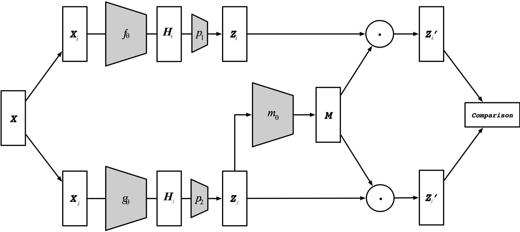
Figure 2: Illustration of the architecture in CLAWS.

A vast majority of the modern unsupervised learning research has been driven by contrastive learning and similar self-supervised learning procedures. Contrastive learning is a popular method that learns representations of images without requiring any image labels. We directly build off of the contrastive learning framework SimCLR, presented in A Simple Framework for Contrastive Learning of Visual Representations (Chen et al. 2020a). In SimCLR, each image is transformed into two correlated views. These views are then fed through a base network, ResNet, to represent each view. These representations are then reduced in dimensionality via a Multilayer Perceptron (MLP) and compared using a contrastive loss that maximizes agreement between representations of the same image. We use the same contrastive loss as SimCLR, Normalized Temperature-scaled Cross-Entropy (NT-Xent). This loss is important (Caron et al. 2020) as the contrastive loss removes the notion of instance classes by directly comparing images features while the image transformation defines the invariances encoded in the features.

In this paper, we present an alteration of contrastive learning that uses focus training. We use a method similar to (Chen et al. 2020a) along with the addition of our attention head. This type of an attention head allows us to focus on important generated features for image representation. The procedure we follow consists of two networks, one to generate representations of a given input image and the second to generate representations of a crop image. Representations from the cropped image will be passed to our attention head to focus on important features from both images representations. Lastly, the NT-Xent loss function is applied to these outputs. In addition to contrastive learning, we combine this type of learning with additional supervision to see the performance of this combination of methods while performing image clustering. In essence, we have two additions to SimCLR, the use of a crop model to generate representations of crop images and the conception of an attention model to focus the contrastive loss comparisons.

At a higher level, contrastive learning works by performing deep comparisons on images and backpropagating errors on the framework used to do these image representations. Before we were able to do this type of training, we relied on methods like principal component analysis (Zitko 1994), independent component analysis (Bell and Sejnowski 1995) and self-organizing maps (Kohonen 1998) between other methods that were traditional and more classical but were the key to open the idea of what we have today as deep representation learning methods. While these classical methods help lay a good foundation, there has been a lot of progress in the last few years, and we have numerous methods now that extend the idea behind contrastive learning in different ways. We can start with SimCLR, where the creation of augmented images enforces the training process; Big Self-Supervised Models are Strong Semi-Supervised Learners (SimCLRv2) (Chen et al. 2020b) in which they work with the combination of label amounts and network sizes. SwAV (Caron et al. 2021) takes contrastive learning methodology without having pairwise comparisons. Contrastive Clustering (Li et al. 2020) introduces a cluster-level contrastive head in combination with an instance-level head, and Cluster Analysis with Deep Embeddings and Contrastive Learning (Sundareswaran et al. 2021) uses a three-prolonged approach with an instance-wise contrastive head, a clustering head, and an anchor head to perform efficient image clustering. Although our idea is based on these preceding works, other interesting works ((Bachman, Hjelm, and Buchwalter 2019; van den Oord, Li, and Vinyals 2019; Wu et al. 2018; Hjelm et al. 2019; He et al. 2020; Grill et al. 2020; Chen and He 2021)) have also been proposed that use contrastive learning and bring out different perspectives.

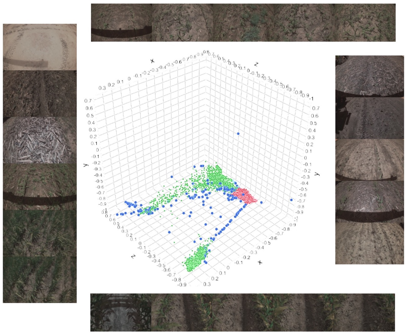
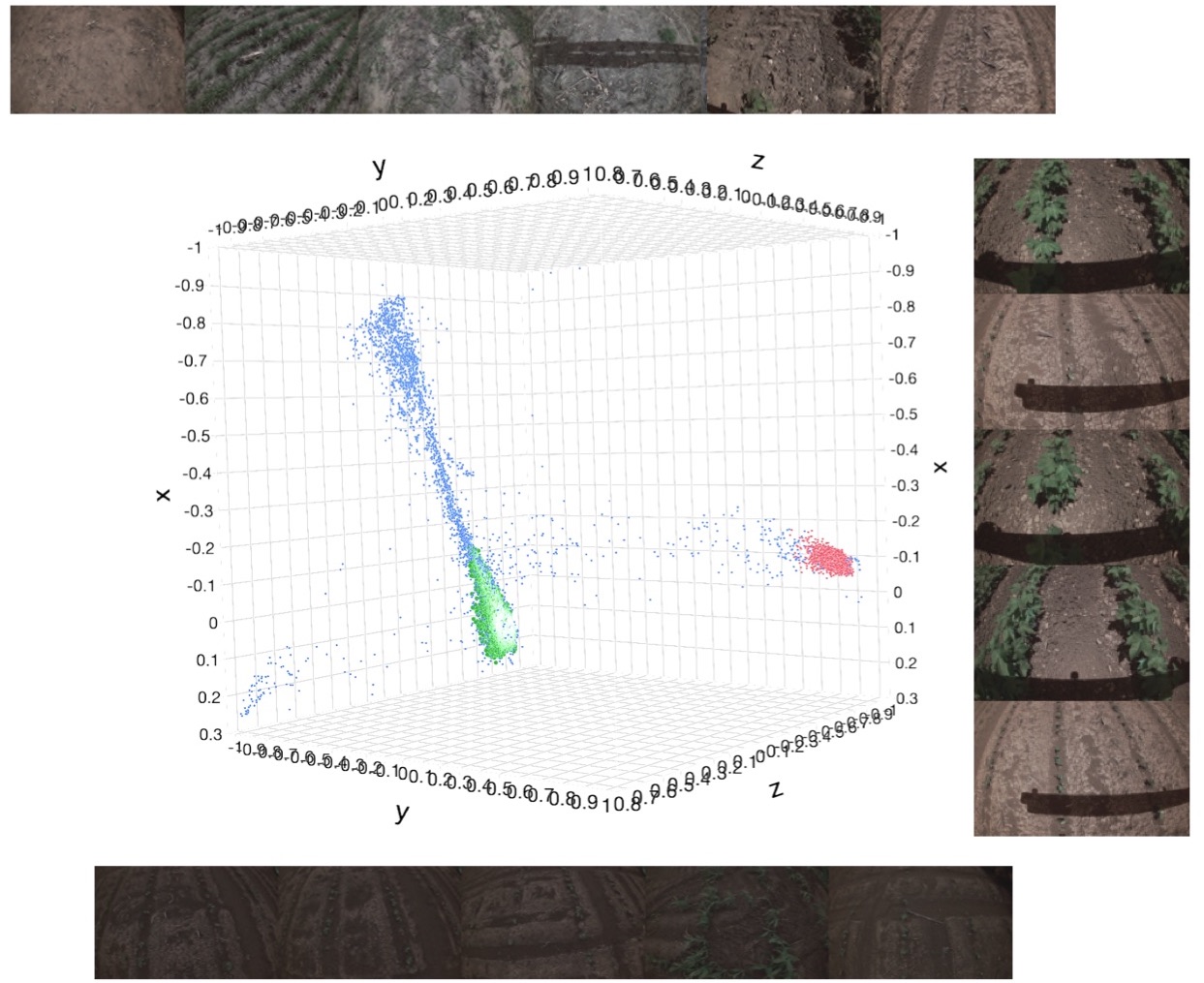
Figure 3: 3D plot containing clusters and outliers (blue) within a specific class. Left represents Corn samples and Right is showing Cotton samples. For Left top and bottom row represents green cluster, images at the right represents red cluster and left represents blue cluster. The Right has a column of images at the right that represents red cluster, bottom images are to show the green cluster and finally the top images represents outliers.

2 Methods

An overview of our model architecture is given in Figure 2. Similar to SimCLR, our method learns representations by maximizing agreement between differently augmented views of the same image. The first augmentation retains the full image size and is fed into a base network that is optimized for full-size images. The second augmentation takes a small crop from the original image and is fed into a base network that is optimized for small crops of images. An attention mask is then applied to both of the representations generated by the base networks, and the attention-filtered representations are then compared using a contrastive loss. The differences between our model and SimCLR can be categorized into 3 major components: 1) the way images are fed into for inference before comparison, 2) the use of two separate base networks instead of one siamese network, and 3) application of an attention mask to the output of each base network before the contrastive loss is calculated. This is also complemented with the use of weak supervision, the two parts of our model (full image network and crop image network) are trained by using cross-entropy loss and NT-Xent.

Our models outputs can be seen as:

$$\textit{{H}}_{i}=f_{\theta}(\textit{{X}}_{i})=\textnormal{EfficientNet}(\textit{{X}}_{i})$$ (1)

$$\textit{{H}}_{j}=g_{\theta}(\textit{{X}}_{j})=\textnormal{EfficientNet}(\textit{{X}}_{j})$$ (2)

were $\textnormal{{X}}_{i}$ and $\textnormal{{X}}_{j}$ are a pair of augmented images drawn from X which is the original image. The hidden layers are $\textit{{H}}_{i}$ and $\textit{{H}}_{j}$ representing the output of the $f_{\theta}$ and $g_{\theta}$, now the hidden layers are then passed to a projection head to produce image representation with 32 features, i.e, $\textnormal{{Z}}_{i}=p_{1}(\textit{{H}}_{i})$ and $\textnormal{{Z}}_{i}=p_{2}(\textit{{H}}_{j})$. To calculate the attention output we send $\textnormal{{Z}}_{i}$ to our attention network $m_{\theta}$ to generate M which is a mask that use to focus training on the important features (further explanation in section 3.3).

2.1 Dataset

The single dataset used for this research is composed of 11 classes of images. Data was obtained while driving over different fields containing one of the possible crops types. A total of 227,060 samples were collected and labeled. The time in which they were collected varies, therefore there is a different variation of lighting over the dataset. The labels of the data are composed by crop fields of Wheat, Cotton, Sorghum, Corn, Peanuts, No crop, Oats, Soybeans, Canola, Sugar, WheatStubble.

2.2 Preprocessing

SimCLR augmented images with a composition of a random crop, random flips (horizontal and vertical), and color distortion. This composition is applied twice to the same image to generate two distinctly augmented images. We follow the same augmentation process, except performing Gaussian blur. We apply two separate augmentation compositions to generate augmented images (full image and crop image). Note that when SimCLR applied random cropping, the crops were always resized to 100x100 to be fed into the base network. Our base networks have different input sizes, so we do not resize images after they are cropped.

We use two distinct base networks, $f_{\theta}$ and $g_{\theta}$ for the full and crop networks respectively. The network used for the full image takes RGB images of size 120x190 as input, while the crop network takes RGB images of size 32x32 as input. Both networks are a standard EfficientNet (Tan and Le 2020) architecture, and both produce output embeddings of the same size, 32 features. Using two separate base networks, rather than feeding both image augmentations through the same base network as SimCLR does, provides two noticeable advantages. First, we do not need to enlarge small crops to fit an architecture, which can produce unintended artifacts in the image. Second, each architecture is more specifically optimized for global or local views.

2.3 Attention Mask

The main innovation in our framework is the incorporation of an attention mask. The mask is generated with a 2-layer perceptron that takes the output of $g_{\theta}$ as input. The output tensors of both $g_{\theta}$ and $f_{\theta}$ are multiplied by this mask before they are compared using a contrastive loss. This created the attention mechanism that we wanted, we created hard attention meaning that the output from the attention head is going to be either 0 or 1 (M). Therefore ${\textbf{Z}^{\prime}}_{i}={\textbf{Z}}_{i}\cdot{\textbf{{M}}}$ and ${\textbf{Z}^{\prime}}_{j}={\textbf{Z}}_{j}\cdot{\textbf{{M}}}$ to then be use to calculate the loss using NT-Xent.

Both base networks need to be able to encode the same concepts in the same corresponding regions of the embeddings they produce. The same mask is applied to both embeddings, so if the output of $g_{\theta}$ contains mainly a strong concept, the mask network will remove out every region except that. If the same region in $f_{\theta}$ output contains a similar concept, then the two embeddings will be very similar after the mask is applied.

3 Results

The models were trained for 300 epochs with a batch size of 55 and an Adam optimizer. We train with this batch size because of the way we were gathering the images for the step, here instead of randomly picking images we specify 5 images per class so that in every step we can train the model in each class.

3.1 Evaluation

To perform evaluation we wanted to focus on the quality of the image representation. Therefore, we compared ours against SimCLR with an adaptation, similar to our model we added a supervised section for it. Now, SimCLR and CLAWS were trained using NT-Xent in combination with supervision by adding an MLP to generate labels from the outputs of the projection head. This way we can do a fair comparison over our agricultural dataset. To evaluate both models after training we did not used the classifier section, we generated the representation of the images, i.e., ran the models over each image up to the output of the projection heads. Given the creation of all the represenation, we pass it to a K-Means clustering method and generated labels for each data point. Finally, we calculated the quality by computing NMI, AMI and ARI scores.

Method	NMI	ARI	AMI
SimCLR	0.6101	0.2873	0.6101
CLAWS(Ours)	0.7325	0.5069	0.7324

In table 1 we can see that our results outperforms SimCLR with supervision. This is also specific for the quality of the represenation of the images. Meaning that by focusing the training with the use of an attention head does helps on focusing on features that relate between the corp image and the full image.

3.2 Gaussian Mixture Models

Furthermore, we implemented Gaussian Mixture Models (GMM) over our image representation. Now we did not used the full dataset, we focus on seeing how our model behaved within a class. To perform this we picked Corn and Cotton and set the output of GMM to be two clusters and an additional one to detect outliers. In figure 3, we can see the output of GMM in the two mentioned crop types. As mentioned before the Left represents Corn and the Right represents Cotton. For Left image the top and bottom row represents green cluster, images at the right represent red cluster and the left represents blue (outliers) cluster. The Right has a column of images at the right that represents red cluster, the bottom images are to show the green cluster, and finally, the top images represent outliers. An important thing to mention about figure 3 is that we are randomly choosing three dimensions from the 32 that represent an image. Therefore, we are not going to see the full relation between clusters in just three dimensions but we can see that even with the use of the raw representation there is a relation preserved in the plot.

Focusing on outliers is our main reason for using GMM, having the ability to generate image representation on then pass it to these models to detect outliers can help in the reduction of the inspection time. It also allows fast customization depending on the task, because it is an unsupervised method, we can change the cluster dimensions and get fast results from it. An example of its use can be seen in figure 3, Left contains 19,792 samples of Corn the GMM detects 315 outliers in which if we inspect them, images that have residue on the ground, are empty, the crop wrongly planted or bad image capture. This means that even when the model generates a similar representation for a specific class, we can detect, within a class, bad samples. Another example, Right shows samples from Cotton, with 66,053 samples and GMM detected 3,401 outliers in which we can also see that for both classes the outliers resemble. Here, again, the images were empty, not correctly taken, contain residues and bad plantation. In addition to GMM clusters, if we talk about the other clusters, we can notice that there is no big issue separating them. The reason to be separated is that these crops can be going through a different stage of growth or other reasons. In figure 3, Left top row we see images that contain weeds, the bottom row show images captured closer. On the Right bottom, we notice images with tire marks on the ground. Therefore, they are assigned to another cluster (within a class) because of many reasons (leaf size, plant height, and image brightness between other factors).

4 Conclusion

This work built upon SimCLR to achieve better representations of images using contrastive learning combined with supervision. Our framework incorporated two distinct base networks and an attention mask, which allowed the network to learn and recognize parts that strongly represent images. With this methodology, we created CLAWS and were able to show encouraging results within class clusters. Further work on this relies on completely unsupervised training.

References

- Bachman, Hjelm, and Buchwalter (2019) Bachman, P.; Hjelm, R. D.; and Buchwalter, W. 2019. Learning Representations by Maximizing Mutual Information Across Views.
- Bell and Sejnowski (1995) Bell, A. J.; and Sejnowski, T. J. 1995. An Information-Maximization Approach to Blind Separation and Blind Deconvolution. Neural Comput. 7(6): 1129–1159. ISSN 0899-7667. doi:10.1162/neco.1995.7.6.1129. URL https://doi.org/10.1162/neco.1995.7.6.1129.
- Caron et al. (2020) Caron, M.; Misra, I.; Mairal, J.; Goyal, P.; Bojanowski, P.; and Joulin, A. 2020. Unsupervised Learning of Visual Features by Contrasting Cluster Assignments. In Larochelle, H.; Ranzato, M.; Hadsell, R.; Balcan, M. F.; and Lin, H., eds., Advances in Neural Information Processing Systems, volume 33, 9912–9924. Curran Associates, Inc. URL https://proceedings.neurips.cc/paper/2020/file/70feb62b69f16e0238f741fab228fec2-Paper.pdf.
- Caron et al. (2021) Caron, M.; Misra, I.; Mairal, J.; Goyal, P.; Bojanowski, P.; and Joulin, A. 2021. Unsupervised Learning of Visual Features by Contrasting Cluster Assignments.
- Chen et al. (2020a) Chen, T.; Kornblith, S.; Norouzi, M.; and Hinton, G. 2020a. A Simple Framework for Contrastive Learning of Visual Representations.
- Chen et al. (2020b) Chen, T.; Kornblith, S.; Swersky, K.; Norouzi, M.; and Hinton, G. 2020b. Big Self-Supervised Models are Strong Semi-Supervised Learners. arXiv preprint arXiv:2006.10029 .
- Chen and He (2021) Chen, X.; and He, K. 2021. Exploring Simple Siamese Representation Learning. In CVPR.
- Grill et al. (2020) Grill, J.; Strub, F.; Altché, F.; Tallec, C.; Richemond, P. H.; Buchatskaya, E.; Doersch, C.; Pires, B. Á.; Guo, Z. D.; Azar, M. G.; Piot, B.; Kavukcuoglu, K.; Munos, R.; and Valko, M. 2020. Bootstrap Your Own Latent: A New Approach to Self-Supervised Learning. CoRR abs/2006.07733. URL https://arxiv.org/abs/2006.07733.
- He et al. (2020) He, K.; Fan, H.; Wu, Y.; Xie, S.; and Girshick, R. 2020. Momentum Contrast for Unsupervised Visual Representation Learning.
- Hjelm et al. (2019) Hjelm, R. D.; Fedorov, A.; Lavoie-Marchildon, S.; Grewal, K.; Bachman, P.; Trischler, A.; and Bengio, Y. 2019. Learning deep representations by mutual information estimation and maximization. In International Conference on Learning Representations. URL https://openreview.net/forum?id=Bklr3j0cKX.
- Kohonen (1998) Kohonen, T. 1998. The self-organizing map. Neurocomputing 21(1): 1–6. ISSN 0925-2312. doi:https://doi.org/10.1016/S0925-2312(98)00030-7. URL https://www.sciencedirect.com/science/article/pii/S0925231298000307.
- Li et al. (2020) Li, Y.; Hu, P.; Liu, Z.; Peng, D.; Zhou, J. T.; and Peng, X. 2020. Contrastive Clustering.
- Sundareswaran et al. (2021) Sundareswaran, R.; Herrera-Gerena, J.; Just, J.; and Jannesari, A. 2021. Cluster Analysis with Deep Embeddings and Contrastive Learning.
- Tan and Le (2020) Tan, M.; and Le, Q. V. 2020. EfficientNet: Rethinking Model Scaling for Convolutional Neural Networks.
- van den Oord, Li, and Vinyals (2019) van den Oord, A.; Li, Y.; and Vinyals, O. 2019. Representation Learning with Contrastive Predictive Coding.
- Wu et al. (2018) Wu, Z.; Xiong, Y.; Yu, S.; and Lin, D. 2018. Unsupervised Feature Learning via Non-Parametric Instance-level Discrimination.
- Zitko (1994) Zitko, V. 1994. Principal component analysis in the evaluation of environmental data. Marine Pollution Bulletin 28(12): 718–722. ISSN 0025-326X. doi:https://doi.org/10.1016/0025-326X(94)90329-8. URL https://www.sciencedirect.com/science/article/pii/0025326X94903298.