Training Experimentally Robust and Interpretable Binarized Regression Models Using Mixed-Integer Programming

Abstract

In this paper, we explore model-based approach to training robust and interpretable binarized regression models for multiclass classification tasks using Mixed-Integer Programming (MIP). Our MIP model balances the optimization of prediction margin and model size by using a weighted objective that: minimizes the total margin of incorrectly classified training instances, maximizes the total margin of correctly classified training instances, and maximizes the overall model regularization. We conduct two sets of experiments to test the classification accuracy of our MIP model over standard and corrupted versions of multiple classification datasets, respectively. In the first set of experiments, we show that our MIP model outperforms an equivalent Pseudo-Boolean Optimization (PBO) model and achieves competitive results to Logistic Regression (LR) and Gradient Descent (GD) in terms of classification accuracy over the standard datasets. In the second set of experiments, we show that our MIP model outperforms the other models (i.e., GD and LR) in terms of classification accuracy over majority of the corrupted datasets. Finally, we visually demonstrate the interpretability of our MIP model in terms of its learned parameters over the MNIST dataset. Overall, we show the effectiveness of training robust and interpretable binarized regression models using MIP.

I Introduction

Machine learning models have significantly improved the ability of autonomous systems to solve challenging tasks, such as image recognition [1], speech recognition [2] and natural language processing [3]. The rapid deployment of such models in safety critical systems resulted in an increased interest in the development of machine learning models that are robust and interpretable [4].

In the context of machine learning, robustness refers to the performance stability of the model in the presence of natural and/or adversarial changes [5]. For example, random noise in the training dataset, or random changes in the environment can both significantly degrade the testing accuracy of a machine learning model when they are not accounted for [6]. Orthogonal to robustness, interpretability is concerned with the insights that the learned model can provide to its users about the relationships that are present in the dataset or the model [7]. Interpretable models are desirable as they often drive actions and further discoveries. Interpretable machine learning aims to construct models that are low in complexity (i.e., typically measured by the size of the model), highly simulatable (i.e., how easy for the user to simulate the prediction of the model), and highly modular (i.e., can each subcomponent of the model be evaluated separately). Interpretable machine learning can be thought of as a set of criteria that should be considered prior to the model selection.

In this paper, we train interpretable machine learning models that are experimentally robust to random corruptions in the dataset. Specifically, we focus on performing the supervised multiclass classification task, and limit our scope to random corruption of labels. Based on the interpretability criteria (i.e., complexity, simulatability and modularity), we select binarized Linear Regression as the appropriate machine learning model, and optimally learn its parameters by solving an equivalent Mixed-Integer Programming (MIP) model. We experimentally demonstrate the performance benefit of training a binarized Linear Regression model using MIP over both standard and corrupted datasets, and visually validate the interpretability of the learned model using the MNIST dataset. Overall, we contribute to the interpretable machine learning literature with an experimentally robust training methodology using MIP.

II Preliminaries

We begin this section by presenting the notation that is used throughout the paper, proceed with the definition of the supervised multiclass classification task, and conclude with a brief introduction of the notions of data corruption and interpretability in machine learning.

II-A Notation

• $F=\{1,\dots,n\}$ is the set of features for positive integer $n\in\mathbb{Z_{+}}$.

• $C=\{1,\dots,m\}$ is the set of classes for positive integer $m\in\mathbb{Z_{+}}$.

• $I=\{1,\dots,k\}$ and $J=\{k+1,\dots,k+l\}$ are the sets of training and test instances for positive integers $k\in\mathbb{Z_{+}}$ and $l\in\mathbb{Z_{+}}$, respectively.

• Document description (i.e., input) $\vec{x}_{i}$ is a vector of values for instance $i\in I\cup J$ over the set of features $F$ such that $\vec{x}_{i}=(x_{1,i},\dots,x_{|F|,i})\in\prod^{|F|}_{f=1}D_{f}$ where $D_{f}$ is the domain of input for feature $f\in F$. In this paper, we assume the domains of input for all features $f\in F$ are binary (i.e., $D_{f}=\{0,1\}$ for all $f\in F$).

• $l_{i}\in C$ is the label for instance $i\in I\cup J$.

• $D=\{d_{1},\dots,d_{|I\cup J|}\}$ is the dataset such that $d_{i}=\langle\vec{x}_{i},l_{i}\rangle$ for instance $i\in I\cup J$.

II-B Multiclass Classification

Given dataset $D$, (supervised) multiclass classification is the task of constructing a function $\mathbb{f}:\{0,1\}^{|F|}\rightarrow C$ using the training dataset $\{d_{1},\dots,d_{|I|}\}$ to correctly predict the label $l_{j}\in C$ of input $\vec{x}_{j}$ for test instances $j\in J$ such that $\mathbb{f}(\vec{x}_{j})=l_{j}$.

Multiclass classification task is commonly solved using models that optimize primarily the training accuracy of function $\mathbb{f}$ that can be defined as $\frac{|\{i|\mathbb{f}(\vec{x}_{i})=l_{i},i\in I\}|}{|I|}$ and secondarily the complexity of function $\mathbb{f}$ that is typically measured by the number of (non-zero) parameters of function $\mathbb{f}$. Intuitively, maximization of training accuracy aims to learn the relationship between input $\vec{x}_{i}$ and label $l_{i}\in C$ while the minimization of complexity aims to select the simplest function $\mathbb{f}$. It has been experimentally shown that the combined optimization of these two objectives can learn function $\mathbb{f}$ with higher test accuracy (i.e., compared to the optimization of the training accuracy by itself) by avoiding overfitting of function $\mathbb{f}$ to the training instances [8].

In many settings, however, the training dataset might be corrupted which can lower the test accuracy of function $\mathbb{f}$. In this paper, we focus on learning accurate function $\mathbb{f}$ that is experimentally robust to corrupted training datasets, and briefly cover data corruption in machine learning next.

II-C Data Corruption in Machine Learning

In the context of machine learning, data corruption refers to modifications to input $\vec{x}_{i}$ and/or label $l_{i}\in C$ of training instance $i\in I$. The nature of such modifications can be due to random noise and/or adversarial attacks, which can significantly lower the test accuracy of function $\mathbb{f}$ [9]. In this paper, we focus on learning accurate function $\mathbb{f}$ that is experimentally robust to random corruption of labels.

In machine learning, experimental accuracy and experimental robustness are both considered as important objectives to measure the performance of function $\mathbb{f}$, and have mainly driven the research to solve challenging tasks, such as image recognition [1], speech recognition [2] and natural language processing [3]. However, such performance increase often came at a price of interpretability of the learned function $\mathbb{f}$. Orthogonal to the previously covered performance-related objectives, interpretability is concerned with the insights function $\mathbb{f}$ provides to its users about relationships that are present in the dataset $I\cup J$ or the learned function $\mathbb{f}$ [7]. In this paper, we focus on learning an interpretable function $\mathbb{f}$, and briefly cover interpretable machine learning next.

II-D Interpretable Machine Learning

Interpretable machine learning is the extraction of knowledge from function $\mathbb{f}$ regarding relationships that are present in the dataset $I\cup J$ or learned by the function $\mathbb{f}$ [7]. The knowledge extracted by function $\mathbb{f}$ is deemed to be relevant if it provides insight for its users about the underlying problem it solves. These insights often drive actions and discovery, and can be communicated through visualization, natural language, or mathematical equations as we will demonstrate in Section IV-D. In this paper, the following interpretability criteria are applied in the modeling stage of our approach to construct function $\mathbb{f}$ [7]:

1. Complexity: Interestingly, complexity has a dual role in both improving the test accuracy (as previously discussed in Section II-B) and the interpretability of function $\mathbb{f}$. That is, when the learned function $\mathbb{f}$ has sufficiently small number of non-zero parameters, the user can understand how the learned parameters relate the input $\vec{x}_{i}$ to the label $l_{i}\in C$ for instance $i\in I\cup J$.

2. Simulatability: A function $\mathbb{f}$ is considered to be simulatable if the user can internalize the entire prediction process of function $\mathbb{f}$ (e.g., if the user can predict the label $l_{i}\in C$ given the input $\vec{x}_{i}$ for function $\mathbb{f}$). Since simulatability requires the entire prediction process of function $\mathbb{f}$ to be internalized by the user, the computations required to make a prediction must be both simple and small in size.

3. Modularity: A function $\mathbb{f}$ is considered to be modular if the subcomponents of function $\mathbb{f}$ can be interpreted independently.

III Training Robust and Interpretable Binarized Regression Models

In this section, we first describe our model assumptions and choices, and then present two equivalent models based on Mixed-Integer Programming (MIP) and Pseudo-Boolean Optimization (PBO) for training interpretable binarized regression models to perform the multiclass classification task.

III-A Model Assumptions and Choices

In this section, we describe our model assumptions and choices to perform the multiclass classification task. One fundamental assumption we make in this paper is the existence of a function $\mathbb{g}:\{0,1\}^{|F|}\rightarrow\mathbb{Z}^{|C|}$ such that $\mathbb{f}(\vec{x}_{i})=\arg\max\mathbb{g}(\vec{x}_{i})$ holds for all instances $i\in I\cup J$ [5]. This assumption has two important benefits for effectively modeling the multiclass classification task.

The first benefit is that it allows us to learn function $\mathbb{g}$ as a binarized Linear Regression model of the form:

$$\mathbb{g}(\vec{x}_{i})=\sum_{f\in F}\vec{w}_{f}x_{f,i}+\vec{b}\quad\forall{i\in I}$$ (1)

where $\vec{w}_{f}\in\{-1,0,1\}^{|C|}$ and $\vec{b}\in\mathbb{Z}^{|C|}$. Based on the interpretability criteria that are previously listed in Section II-D, the binarized Linear Regression model can be considered one of the most interpretable machine learning models. The binarized Linear Regression model has:

1. low complexity because it has no latent parameters (c.f., Deep Neural Networks [10]) and can easily be regularized,

2. high simulatability due to the binarization of the domain of the weight parameters $\vec{w}_{f}\in\{-1,0,1\}^{|C|}$ which gives each value an intuitive semantic meaning (i.e., negative impact: -1, no impact: 0 and positive impact: 1) for the prediction of a given class $c\in C$. Moreover, it utilizes only simple additive features that require at most linear number of addition operations (in the size of $|F|$) per class $c\in C$ to make its predictions, and

3. high modularity due to the independence of computations carried for each output of function $\mathbb{g}$.

The second benefit is that it allows us to optimize the total margin by which the training instances $I$ are correctly and incorrectly classified. We will experimentally demonstrate in Section IV-C that this optimization allows us to learn function $\mathbb{f}$ that is robust to corrupted training datasets.

Next, we present two equivalent models based on Mixed-Integer Programming (MIP) and Pseudo-Boolean Optimization (PBO) for training robust and interpretable binarized regression models, that are based on our modeling assumptions and choices, to perform the multiclass classification task.

III-B Mixed-Integer Programming Model

In this section, we present the Mixed-Integer Programming (MIP) model to train a binarized regression model to perform the multiclass classification task.

Hyperparameters

The MIP model uses the following hyperparameters:

• $\alpha\in\mathbb{R_{+}}$ is the hyperparameter representing the importance of maximizing the total margin of correctly classified training instances.

• $\beta\in\mathbb{R_{+}}$ is the hyperparameter representing the importance of minimizing the total margin of incorrectly classified training instances.

Decision Variables

The MIP model uses the following decision variables:

• $w^{+}_{f,c}\in\{0,1\}$ and $w^{-}_{f,c}\in\{0,1\}$ together encode the value of the weight between feature $f\in F$ and class $c\in C$.

• $b_{c}\in\mathbb{Z}$ encodes the value of the bias for class $c\in C$.

• $y_{c,i}\in\mathbb{Z}$ encodes the value of the prediction for class $c\in C$ and training instance $i\in I$.

• $e^{+}_{i}\in\mathbb{Z_{+}}$ and $e^{-}_{i}\in\mathbb{Z_{+}}$ encode the value of the margin for (i) correctly and (ii) incorrectly classifying training instance $i\in I$, respectively.

Constraints

The MIP model uses the following constraints:

$$w^{+}_{f,c}+w^{-}_{f,c}\leq 1 \forall{f\in F,c\in C}$$ (2)

$$\sum_{f\in F}(w^{+}_{f,c}-w^{-}_{f,c})x_{f,i}+b_{c}=y_{c,i} \forall{c\in C,i\in I}$$ (3)

$$y_{l_{i},i}\geq y_{c,i}+e^{+}_{i}-e^{-}_{i} \forall{i\in I,c\in C\setminus l_{i}}$$ (4)

$$e^{+}_{i}\geq 0,e^{-}_{i}\geq 0 \forall{i\in I}$$ (5)

$$w^{+}_{f,c},w^{-}_{f,c}\in\{0,1\} \forall{f\in F,c\in C}$$ (6)

$$e^{+}_{i},e^{-}_{i}\in\mathbb{Z} \forall{i\in I}$$ (7)

$$y_{c,i}\in\mathbb{Z} \forall{c\in C,i\in I}$$ (8)

$$b_{c}\in\mathbb{Z} \forall{c\in C}$$ (9)

where constraint (2) ensures that the weight between feature $f\in F$ and class $c\in C$ cannot be both positive and negative, constraint (3) computes the prediction as the weighted sum of its inputs plus the bias for class $c\in C$ and training instance $i\in I$, constraint (4) relates the prediction of all classes $C$ to the margin of correctly and incorrectly classifying training instance $i\in I$, constraint (5) enforces the margin of correctly and incorrectly classifying training instance $i\in I$ to be non-negative and constraints (6-9) define the domain of all decision variables.

Objective Function

The MIP model uses the following objective function:

$$\min\;-\alpha\sum_{i\in I}e^{+}_{i}+\beta\sum_{i\in I}e^{-}_{i}+\sum_{f\in F,c\in C}(w^{+}_{f,c}+w^{-}_{f,c})$$ (10)

which balances the optimization of prediction margin and model size by (i) maximizing the total margin of correctly classified training instances, (ii) minimizing the total margin of incorrectly classified training instances and (iii) minimizing the total model size.

III-C Pseudo-Boolean Optimization Model

In this section, we present the Pseudo-Boolean Optimization (PBO) model to train a binarized regression model to perform the multiclass classification task.

Hyperparameters

The PBO model uses the same sets of hyperparameters as the previously presented MIP model in addition to hyperparameter $Q$ that is used to quantize the domains of integer-valued decision variables.

Decision Variables, Constraints and Objective Function

The PBO model uses the same sets of decision variables as the previously presented MIP model to encode the weights $w^{+}_{f,c}\in\{0,1\}$ and $w^{-}_{f,c}\in\{0,1\}$. Given PBO is restricted to have decision variables with only binary domains, the PBO model uses a set of decision variables $b_{c,q}\in\{0,1\}$, $y_{c,i,q}\in\{0,1\}$, $e^{+}_{i,q}\in\{0,1\}$ and $e^{-}_{i,q}\in\{0,1\}$ to equally represent the domains of decision variables $b_{c}\in\mathbb{Z}$, $y_{c,i}\in\mathbb{Z}$, $e^{+}_{i}\in\mathbb{Z_{+}}$ and $e^{-}_{i}\in\mathbb{Z_{+}}$, respectively. The domain of some (bounded) decision variable $x\in\mathbb{Z}$ is represented using the following formula:

$$x=x_{LB}+\sum_{q=1}^{Q}2^{q-1}x_{q}$$ (11)

together with the following constraint:

$$x_{LB}+\sum_{q=1}^{Q}2^{q-1}x_{q}\leq x_{UB}$$ (12)

where $x_{LB}$ and $x_{UB}$ represent the lower bound and the upper bound on decision variable $x$, and the value of hyperparameter $Q$ is calculated according to the following formula:

$$Q=\left\lceil{\log_{2}(x_{UB}-x_{LB}+1)}\right\rceil$$ (13)

Finally, the PBO model uses the same sets of constraints and the objective function as the previously presented MIP model with the minor modification that encodes the set of decision variables $b_{c}\in\mathbb{Z}$, $y_{c,i}\in\mathbb{Z}$, $e^{+}_{i}\in\mathbb{Z_{+}}$ and $e^{-}_{i}\in\mathbb{Z_{+}}$ according to formula (11), formula (13) and constraint (12) using the set of decision variables $b_{c,q}\in\{0,1\}$, $y_{c,i,q}\in\{0,1\}$, $e^{+}_{i,q}\in\{0,1\}$ and $e^{-}_{i,q}\in\{0,1\}$.

IV Experimental Results

In this section, we begin by presenting the results of two sets of computational experiments. In the first set of experiments, we test the effectiveness of training a binarized regression model to perform the multiclass classification task using our MIP and PBO models against Logistic Regression (LR) with real-valued weights and biases, and Gradient Descent (GD) with binarized weights and integer-valued biases over three standard datasets, namely: MNIST [12], Flags [13] and Ask Ubuntu [14]. We provide detailed comparative results on both the training and test accuracy of all models, and further report the model sizes, runtimes and optimality gaps of our MIP and PBO models. Our detailed results for the first set of experiments show that the MIP model achieves competitive test accuracy results to the real-valued LR model over three datasets and outperforms the LR model in one dataset, while achieving upto around 70% model size reduction. In the second set of experiments, we test the effectiveness of training a binarized regression model to perform the multiclass classification task using our MIP model against the previously described LR and GD models over three corrupted datasets. We provide detailed comparative results on the test accuracy of all models. Our results for the second set of experiments show that our MIP model outperforms the LR model in majority of the corrupted datasets without experiencing significant degradation in test accuracy. We conclude this section by visually demonstrating the interpretability of our MIP model using the interpretability criteria discussed previously in Section II-D.

IV-A Experimental Domains and Setup

The domains and the setup used throughout this section is as follows.

Experimental Domains

The MNIST [12] dataset consists of 784 features and 10 classes with 70,000 instances. The dataset is of grayscale images of handwritten digits represented by 784 pixels (i.e., in 28 by 28 pixel format) where each pixel has a value between 0 and 255. We have binarized each pixel such that the pixel is set to 1 if its value is greater than $\frac{255}{2}$, and 0 otherwise. We trained our models over 20, 60, 100, 200, 300, 500, 700 and 1000 training instances, and reported test accuracy results over the remaining dataset. The Flags [13] dataset consists of 43 features and 5 classes with 143 instances. The dataset describes the attributes of the flags of various countries. We trained our models over 10, 25, 35 and 50 training instances, and reported test accuracy results over the remaining dataset. Finally, the Ask Ubuntu [14] dataset consists of 5 classes with 162 instances. The dataset has five classes which refer to the user’s intent behind the questions asked. Natural language preprocessing is performed to extract the features of this dataset. We trained our models over 10, 23 and 43 training instances, and reported test accuracy results over the remaining dataset. Finally in the second set of experiments, 10% of labels are randomly assigned to a different class, and everything else remained the same. Table I provides a summary of the datasets.

Dataset	$|$F$|$, $|$C$|$	$|$I$|$	$\alpha$, $\beta$	Brief Description
MNIST	784, 10	20, 60,	5, 10	Image classification task
		100, 200,		with grayscale images of
		300, 500,		handwritten digits
		700, 1000		represented by 784 pixels
				(i.e., in 28 by 28 format).
Flags	43, 5	10, 25,	2, 5	Describes the attributes
		35, 50		of the flags of countries.
Ubuntu	48	10	2, 5	Natural language processing
	93	23		task to classify the intention
	153	43		of the user behind the
				question asked.

TABLE I: Summary of the datasets including feature and class sizes, number of training instances used for each training problem, the values of the hyperparameters $\alpha$ and $\beta$, and the brief descriptions of the datasets.

Experimental Setup

All experiments were run on Intel Core i5-8250U CPU 1.60GHz with 8.00 GB memory, using a single thread with one hour total time limit per training problem. The MIP model is optimized using Gurobi [15], the PBO model is optimized using RoundingSat [16], the LR model is optimized using Scikit-learn [17] and the GD model is created using LARQ [18] and trained with a learning rate of 0.001 over 200 epochs using Adam [19]. The value of hyperparameter $\alpha$ is selected using grid search where the value of hyperparameter $\beta$ is set to $2\alpha$. Both MIP and PBO models used the same selected values of hyperparameters $\alpha$ and $\beta$ as detailed in Table I.

IV-B Experiment 1: Training with Standard Datasets

In the first set of experiments, we compare the effectiveness of performing the multiclass classification task using the MIP model and the PBO model against LR and GD over the standard datasets. Figure 1 visualizes the training accuracy (i.e., the left column) and the test accuracy (i.e., the right column) of all models over each dataset (i.e., represented by individual rows). Table II compares the model sizes, runtimes and optimality gaps of both MIP and PBO models.

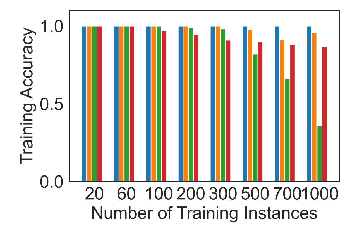
(a) Standard MNIST

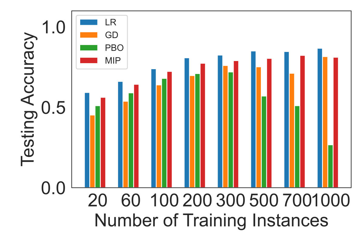
(b) Standard MNIST

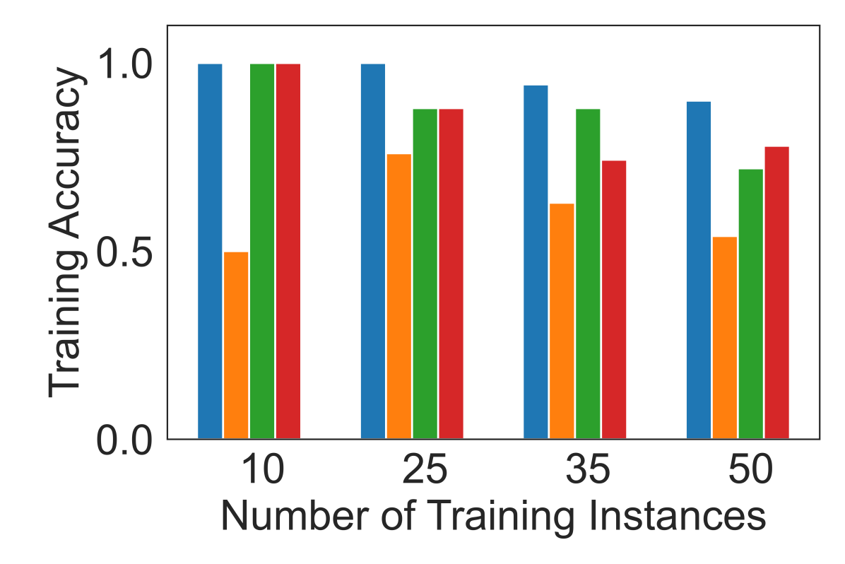
(c) Standard Flags

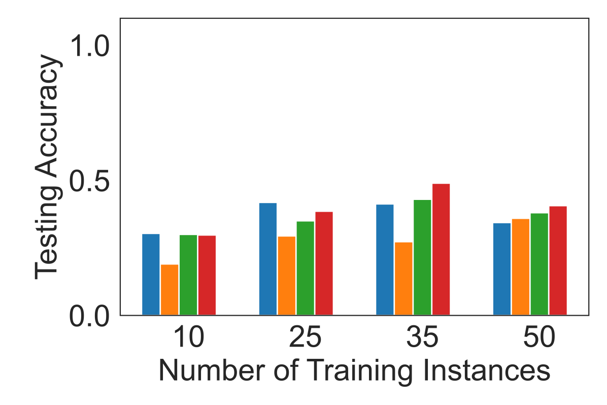
(d) Standard Flags

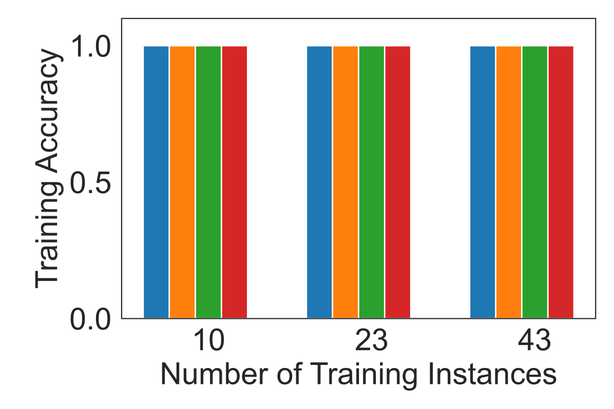
(e) Standard Ask Ubuntu

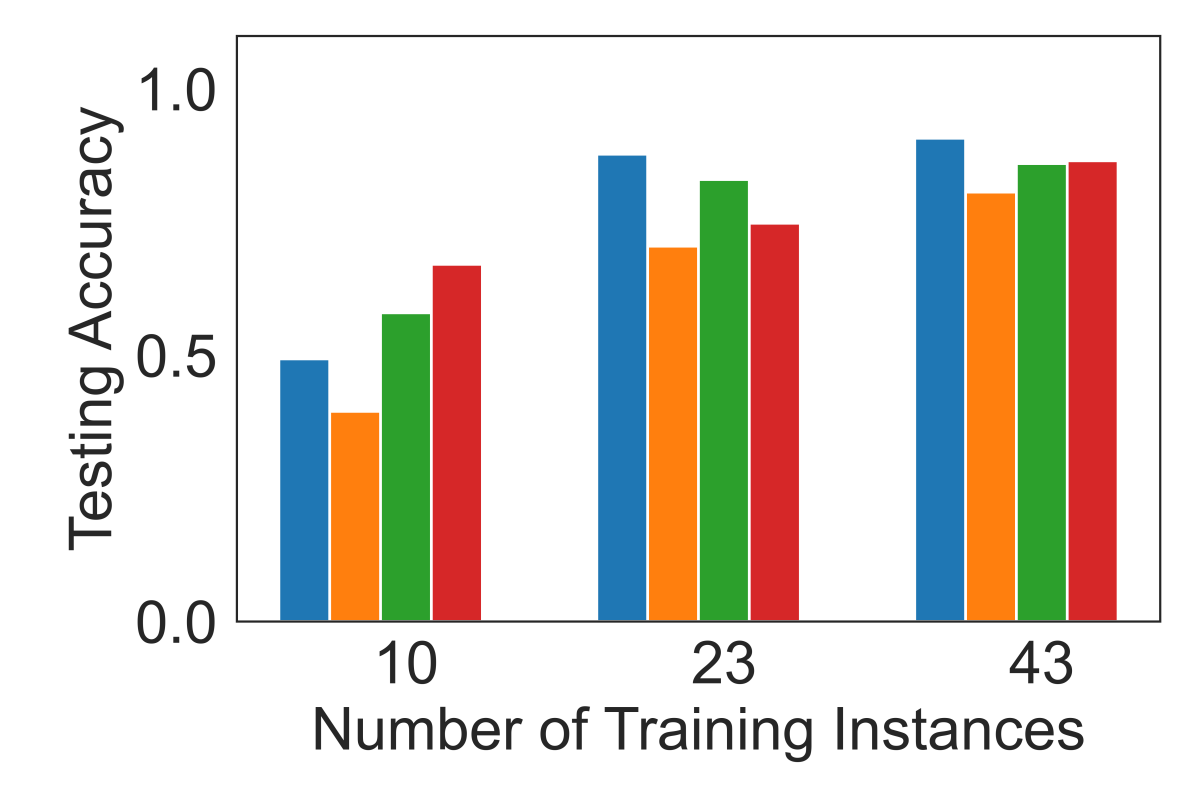
(f) Standard Ask Ubuntu

Figure 1: Visualization of Experiment 1 which compares the training accuracy (left) and the test accuracy (right) of the MIP model (red) and the PBO model (green) against the LR model (blue) and the GD model (orange) over three standard datasets and different number of training instances within one hour time limit.

In Figure 1, the inspection of subfigures 1(a) and 1(b) highlights the clear capability of the MIP model to scale with the increasing size of the training datasets. In the MNIST dataset, the MIP model outperforms the binarized GD model in 7 out of 8 training problems in terms of testing accuracy, and performs competitively with the real-valued LR model. In contrast to the MIP model, the performance of the PBO model degrades with the increasing number of training instances. Moreover, the inspection of subfigures 1(c), 1(d), 1(e) and 1(f) demonstrates the ability of both the MIP model and the PBO model to train models with competitive test accuracies over small training problems. In Flags and Ask Ubuntu datasets, the MIP model and the PBO model consistently outperform the binarized GD model in terms of testing accuracy, and perform competitively with the real-valued LR model.

Model	Dataset, $|$I$|$	Gap	Time (sec.)	Reduction (%)
MIP	MNIST, 20	0.00	3.99	62.19
PBO	MNIST, 20	0.34	x $\geq$ T.O.	3.48
MIP	MNIST, 60	0.00	304.87	55.23
PBO	MNIST, 60	0.52	T.O.	11.28
MIP	MNIST, 100	0.00034	T.O.	49.72
PBO	MNIST, 100	0.51	T.O.	17.48
MIP	MNIST, 200	0.00063	T.O.	44.87
PBO	MNIST, 200	0.85	T.O.	34.22
MIP	MNIST, 300	0.00068	T.O.	43.52
PB	MNIST, 300	1.28	T.O.	31.98
MIP	MNIST, 500	0.00078	T.O.	40.47
PBO	MNIST, 500	9.76	T.O.	19.97
MIP	MNIST, 700	0.0010	T.O.	39.31
PBO	MNIST, 700	12.60	T.O.	15.30
MIP	MNIST, 1000	0.00081	T.O.	37.33
PBO	MNIST, 1000	140.89	T.O.	6.54
MIP	Flags, 10	0.00	0.13	69.77
PBO	Flags, 10	0.00	22.00	53.48
MIP	Flags, 25	0.00	0.71	48.37
PBO	Flags, 25	96.25	T.O.	51.62
MIP	Flags, 35	0.00	0.58	41.40
PBO	Flags, 35	72.03	T.O.	47.44
MIP	Flags, 50	0.00	2.43	44.19
PB	Flags, 50	119.56	T.O.	37.67
MIP	Ubuntu, 10	0.00	0.11	69.58
PBO	Ubuntu, 10	0.00	13.16	28.75
MIP	Ubuntu, 23	0.00	0.35	68.17
PBO	Ubuntu, 23	0.00	1192.20	33.54
MIP	Ubuntu, 43	0.00	0.83	65.88
PBO	Ubuntu, 43	251.08	T.O.	31.50

TABLE II: Comparison of the MIP model and the PBO model in terms of their duality gaps, runtimes and model size reductions in Experiment 1 where T.O. means timeout.

The inspection of Table II highlights the benefit of using the MIP model over the PBO model for training binarized regression models. Across all training problems, the MIP model outperforms the PBO model in terms of runtime performance where the PBO model almost always runs out of the one hour time limit. As a result, the PBO model can return feasible solutions with large duality gaps that can yield low testing accuracy (e.g., as visualized in subfigure 1(b)).

IV-C Experiment 2: Training with Corrupted Datasets

In the second set of experiments, we compare the effectiveness of performing the multiclass classification task using the MIP model against LR and GD models over corrupted datasets. Figure 2 visualizes the test accuracy of all three models over each corrupted dataset (i.e., represented by individual rows) as well as the decrease in test accuracy that is due to data corruption, which is measured by the difference between the test accuracy of a given model in Experiment 1 and Experiment 2.

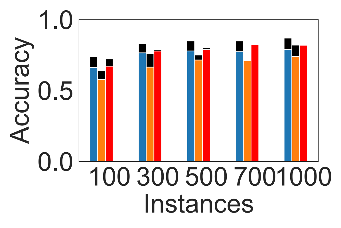
(a) Corrupted MNIST

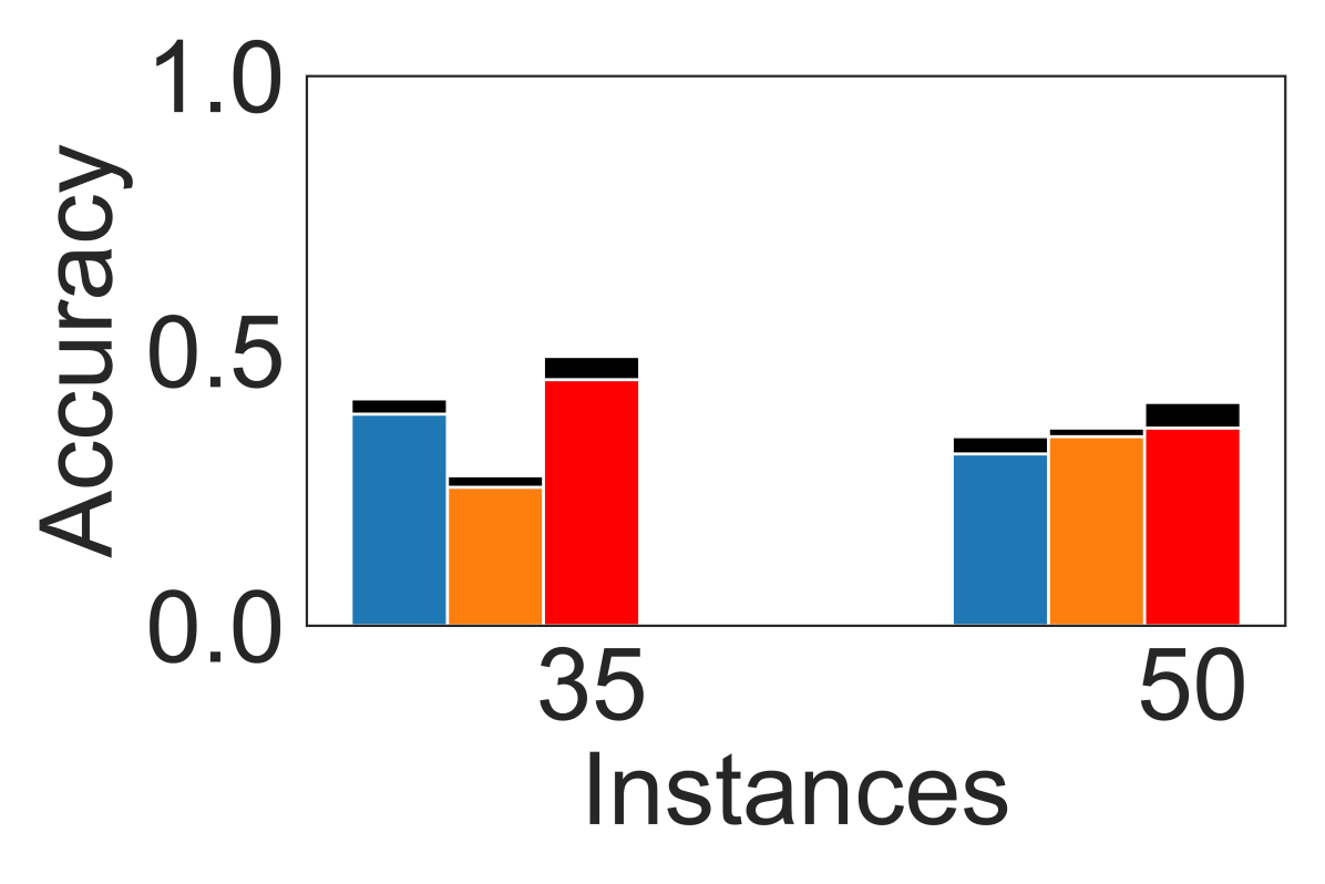
(b) Corrupted Flags

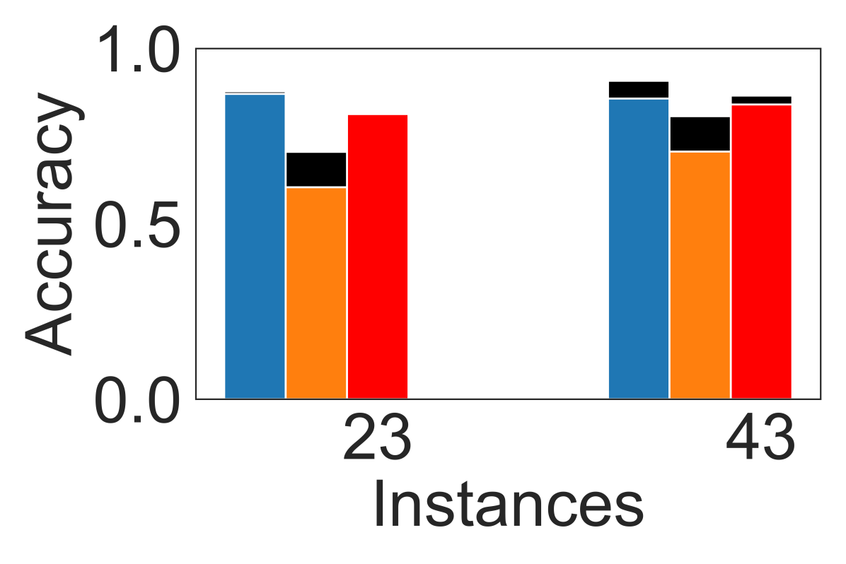
(c) Corrupted Ask Ubuntu

Figure 2: Visualization of Experiment 2 which compares the test accuracy of the MIP model (red) against the LR model (blue) and the GD model (orange) over three corrupted datasets and different number of training instances within one hour time limit. For each model, the black region represents the decrease in test accuracy due to random corruption of labels.

In Figure 2, the inspection of subfigures 2(a), 2(b) and 2(c) demonstrates the experimental robustness of the MIP model over both LR and GD models across all three corrupted datasets. In the corrupted MNIST and Flags datasets, the MIP model outperforms both LR and GD models with minimal decrease in its testing accuracy. Similarly in the corrupted Ask Ubuntu dataset, the MIP model outperforms the GD model while performing competitively with the LR model.

Overall, our results highlight the clear performance benefit of training binarized regression models for the multiclass classification task using MIP. Next, we turn our attention to the interpretability our MIP model.

IV-D Interpretability Results

In this section, we focus on the interpretability of our MIP model based on the criteria that are previously discussed in Section II-D, namely: complexity, simulatability and modularity. Given the binarized regression model is highly modular by definition (i.e., each output of the regression model can be computed independently from the others), we focus on the remaining two criteria.

Complexity

As evident from Table II, our MIP model often learns binarized regression models with significantly reduced complexity through near optimal regularization; by setting both decision variables $w^{+}_{f,c}\in\{0,1\}$ and $w^{-}_{f,c}\in\{0,1\}$ equal to 0. Given the learned binarized regression model is often optimally regularized and has no latent parameters by definition, we conclude that the binarized regression model learned by solving our MIP model has low complexity.

Simulatability

In order to demonstrate the simulatability of the learned binarized regression model, we simply visualize the learned non-zero weights of the learned binarized regression model as follows. For each class $c\in C=\{0,1,\dots,9\}$, we color pixel $f\in F=\{0,1,\dots,783\}$ to: black if the value of decision variable $w^{+}_{f,c}$ that is obtained from solving the MIP model is 1, white if the value of decision variable $w^{-}_{f,c}$ that is obtained from solving the MIP model is 1, and gray otherwise. Given the visualization of the learned weights in Figure 3, the users can take any input image and simulate the prediction of the learned model by visually comparing the input image to the subfigures 3(a) to 3(j). Intuitively, each subfigure $c$ visually represents what the learned binarized regression model predicts number $c$ to look like (and not to look like) based on its learned weights.

(a) Number 0

(b) Number 1

(c) Number 2

(d) Number 3

(e) Number 4

(f) Number 5

(g) Number 6

(h) Number 7

(i) Number 8

(j) Number 9

Figure 3: Visualization of interpretability results for MNIST over each number $c\in C=\{0,\dots,9\}$. A pixel is colored to: black if the value of decision variable $w^{+}_{f,c}$ is 1, white if the value of decision variable $w^{-}_{f,c}$ is 1, and gray otherwise. Intuitively, each subfigure $c$ visually represents what the learned binarized regression model predicts number $c$ to look like (and not to look like) based on its learned weights.

V Discussion, Related Work and Future Work

In this section, we discuss our assumptions, choices, contributions and experimental results in relation to the literature with the goal of opening new areas for future work.

In Section III-A, we detailed our model assumptions and choices for training accurate and interpretable binarized models using MIP and PBO. Similar to Rosenfeld et al. [5], we made the assumption on the existence of function $\mathbb{g}$ which allowed us to train linear regression models for the multiclass classification task. In Section IV-B, we experimentally demonstrated that modeling $\mathbb{g}$ instead of $\mathbb{f}$ significantly improves the test performance of our MIP model. Our results suggest that similar works on training Binarized Neural Networks [20] using MIP models [21] might also benefit from similar explicit modeling of function $\mathbb{g}$.

In Section IV-C, we experimentally demonstrated that our learned binarized regression model is robust to random label corruption. Under adversarial settings, the data corruption problem can be formulated as a bilevel optimization problem where the attacker tries to optimally corrupt the dataset in order to degrade the test accuracy of the machine learning model [22]. Under such adversarial settings, the ability to provide formal robustness guarantees [6] presents an important venue for future work. Similar to this paper, the robustness study of other interpretable machine learning models (e.g., decision lists [23], decision sets [24], decision trees [25]) can potentially yield important ideas for future work.

(a) Flags 0

(b) Flags 1

(c) Flags 2

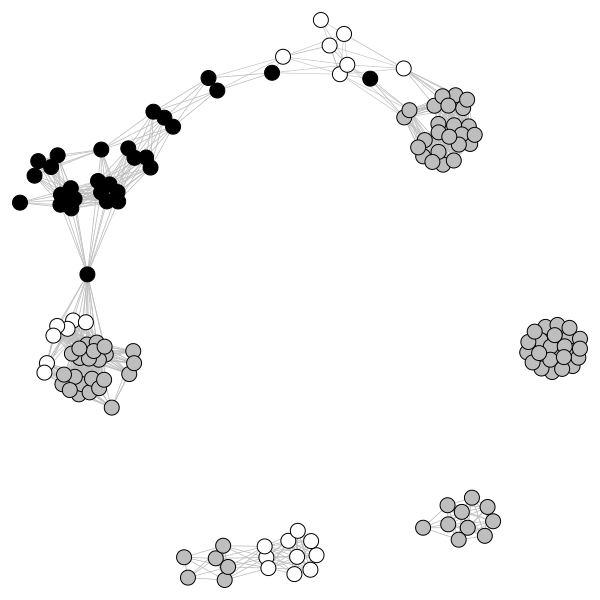
(d) Ubuntu 0

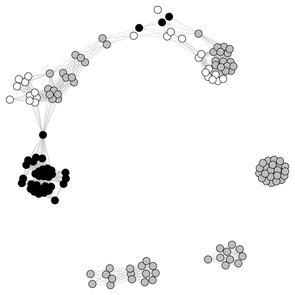
(e) Ubuntu 1

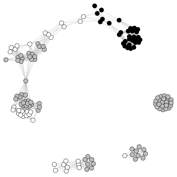
(f) Ubuntu 2

Figure 4: Visualization of interpretability results for Flags and Ask Ubuntu datasets over different classes using the same coloration methodology that is described in Figure 3 where each vertex represents a feature and two vertices are connected by an edge based on their Hamming distance to each other. Here, we have used the Continuous k-Nearest Neighbours method [26] such that an edge is defined for a pair of features $x,y\in F$ if $d(x,y)<\delta*\sqrt{d(x,x_{k})d(y,y_{k})}$ where $d(x,y)$ denotes the Hamming distance between features $x$ and $y$, $\delta\in\mathbb{R_{+}}$ is a parameter controlling the sparsity of the graph, and features $x_{k},y_{k}\in F$ are the k-th nearest neighbours of features $x$ and $y$, respectively.

In Section IV-D, we experimentally demonstrated the interpretability of our learned binarized regression model on a challenging visual task (i.e., MNIST). The effective visualization of our learned models on non-visual tasks (e.g., as visualized in subfigures 4(a)-4(c) and 4(d)-4(e) for Flags and Ask Ubuntu datasets) in order to derive valuable insights remains an important area for future work.

References

- [1] A. Krizhevsky, I. Sutskever, and G. E. Hinton, “Imagenet classification with deep convolutional neural networks,” in 25th NIPS, 2012, pp. 1097–1105.
- [2] L. Deng, G. E. Hinton, and B. Kingsbury, “New types of deep neural network learning for speech recognition and related applications: an overview,” in IEEE International Conference on Acoustics, Speech and Signal Processing, 2013, pp. 8599–8603.
- [3] R. Collobert, J. Weston, L. Bottou, M. Karlen, K. Kavukcuoglu, and P. Kuksa, “Natural language processing (almost) from scratch,” JMLR, vol. 12, pp. 2493–2537, 2011.
- [4] C. Rudin, “Stop explaining black box machine learning models for high stakes decisions and use interpretable models instead,” Nature Machine Intelligence, vol. 1, pp. 206–215, 05 2019.
- [5] E. Rosenfeld, E. Winston, P. Ravikumar, and Z. Kolter, “Certified robustness to label-flipping attacks via randomized smoothing,” in Proceedings of the 37th International Conference on Machine Learning, ser. Proceedings of Machine Learning Research, H. D. III and A. Singh, Eds., vol. 119. PMLR, 13–18 Jul 2020, pp. 8230–8241.
- [6] N. Natarajan, I. S. Dhillon, P. Ravikumar, and A. Tewari, “Learning with noisy labels,” in Proceedings of the 26th International Conference on Neural Information Processing Systems - Volume 1, ser. NIPS’13. Red Hook, NY, USA: Curran Associates Inc., 2013, p. 1196–1204.
- [7] W. J. Murdoch, C. Singh, K. Kumbier, R. Abbasi-Asl, and B. Yu, “Definitions, methods, and applications in interpretable machine learning,” Proceedings of the National Academy of Sciences, vol. 116, no. 44, pp. 22 071–22 080, 2019.
- [8] P. Bhlmann and S. van de Geer, Statistics for High-Dimensional Data: Methods, Theory and Applications. Springer Publishing Company, Incorporated, 2011.
- [9] B. Han, Q. Yao, X. Yu, G. Niu, M. Xu, W. Hu, I. Tsang, and M. Sugiyama, “Co-teaching: Robust training of deep neural networks with extremely noisy labels,” in NeurIPS, 2018, pp. 8535–8545.
- [10] W. S. McCulloch and W. Pitts, “A logical calculus of the ideas immanent in nervous activity,” pp. 115–133, 1943.
- [11] B. Say, “Optimal planning with learned neural network transition models,” Ph.D. dissertation, University of Toronto, Toronto, ON, Canada, 2020.
- [12] Y. LeCun and C. Cortes, “MNIST handwritten digit database,” 2010.
- [13] J. D. Romano, T. T. Le, W. La Cava, J. T. Gregg, D. J. Goldberg, P. Chakraborty, N. L. Ray, D. Himmelstein, W. Fu, and J. H. Moore, “Pmlb v1.0: an open source dataset collection for benchmarking machine learning methods,” arXiv preprint arXiv:2012.00058v2, 2021.
- [14] D. Braun, A. Hernandez-Mendez, F. Matthes, and M. Langen, “Evaluating natural language understanding services for conversational question answering systems,” in Proceedings of the 18th Annual SIGdial Meeting on Discourse and Dialogue. Saarbrücken, Germany: Association for Computational Linguistics, 2017, pp. 174–185.
- [15] L. Gurobi Optimization, “Gurobi optimizer reference manual,” 2021.
- [16] J. Elffers and J. Nordström, “Divide and conquer: Towards faster pseudo-boolean solving,” in Proceedings of the Twenty-Seventh International Joint Conference on Artificial Intelligence, ser. IJCAI’18, 2018, pp. 1291–1299.
- [17] F. Pedregosa, G. Varoquaux, A. Gramfort, V. Michel, B. Thirion, O. Grisel, M. Blondel, P. Prettenhofer, R. Weiss, V. Dubourg et al., “Scikit-learn: Machine learning in python,” Journal of machine learning research, vol. 12, pp. 2825–2830, 2011.
- [18] L. Geiger and P. Team, “Larq: An open-source library for training binarized neural networks,” Journal of Open Source Software, vol. 5, no. 45, p. 1746, Jan. 2020.
- [19] D. P. Kingma and J. Ba, “Adam: A method for stochastic optimization,” 2014, cite arxiv:1412.6980Comment: Published as a conference paper at the 3rd International Conference for Learning Representations, San Diego, 2015.
- [20] I. Hubara, M. Courbariaux, D. Soudry, R. El-Yaniv, and Y. Bengio, “Binarized neural networks,” in Proceedings of the Thirtieth International Conference on Neural Information Processing Systems, ser. NIPS’16, USA, 2016, pp. 4114–4122.
- [21] R. Toro Icarte, L. Illanes, M. P. Castro, A. A. Cire, S. A. McIlraith, and J. C. Beck, “Training binarized neural networks using MIP and CP,” in Principles and Practice of Constraint Programming, T. Schiex and S. de Givry, Eds. Cham: Springer International Publishing, 2019, pp. 401–417.
- [22] Z. Suvak, M. F. Anjos, L. Brotcorne, and D. Cattaruzza, “Design of poisoning attacks on linear regression using bilevel optimization,” 2021.
- [23] R. L. Rivest, “Learning decision lists,” Mach. Learn., vol. 2, no. 3, p. 229–246, Nov. 1987.
- [24] P. Clark and T. Niblett, “The cn2 induction algorithm,” Mach. Learn., vol. 3, no. 4, p. 261–283, 1989.
- [25] L. Breiman, J. H. Friedman, R. A. Olshen, and C. J. Stone, Classification and Regression Trees. Monterey, CA: Wadsworth and Brooks, 1984.
- [26] T. Berry and T. Sauer, “Consistent manifold representation for topological data analysis,” Foundations of Data Science, vol. 1, no. 1, pp. 1–38, 2019.