A benchmark with decomposed distribution shifts for 360 monocular depth estimation
Abstract
In this work we contribute a distribution shift benchmark for a computer vision task; monocular depth estimation. Our differentiation is the decomposition of the wider distribution shift of uncontrolled testing on in-the-wild data, to three distinct distribution shifts. Specifically, we generate data via synthesis and analyze them to produce covariate (color input), prior (depth output) and concept (their relationship) distribution shifts. We also synthesize combinations and show how each one is indeed a different challenge to address, as stacking them produces increased performance drops and cannot be addressed horizontally using standard approaches.
1 Introduction
Data-driven methods are conditioned on the data which are available during the model development but are to be applied on real world data. Considering that the former data distribution is , which is the result of applying a sampling function to the real world distribution . Typically, is separated into different splits and , used to train the model and validate its behaviour respectively, with the latter process driving model selection. A data distribution shift can be described as the condition where the joint distribution of inputs and outputs differs between the training and test stages [1].
This is an actual problem that many practical applications face, affecting their overall performance, robustness and reliability. The phenomenon is more prominent in tasks where annotated data collection is difficult and has been generally addressed in the literature as the domain shift [2] or the generalization of data-driven models [3, 4], or otherwise as out-of-distribution robustness [5]. More information about out-of-distribution (OOD) learning and generalization can be found in recent surveys [6, 7, 8].
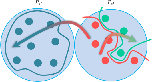
Up to now, most works approach this problem in its general setting via zero-shot cross-dataset transfer experiments that aim at assessing model performance under a general distribution shift, considering two different samplings and , as seen in Figure 1. A recent benchmark [9] provided simultaneously data for sub-population shift, a special case of distribution shifts, and a generic domain generalization shift across a number of datasets and tasks.
In this work, we contribute a novel benchmark for distribution shift performance assessment, in the context of a computer vision task notorious for its complex data collection processes; monocular depth estimation. The novelty of our benchmark lies in the decomposition of generalized shift into components, expressed separately or in combination, via targeted test splits.
2 The Pano3D Dataset
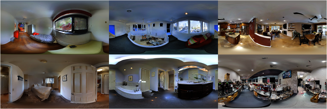
Our benchmark relies on two recent 3D building scan datasets, Matterport3D (M3D) [10] and GibsonV2 (GV2) [11], using modern synthesis to produce high quality spherical panoramas coupled with depth maps. Sample images can be found in Figure 2. Specifically, we use M3D as a traditional in-distribution model development dataset and GV2 as a zero-shot cross-dataset transfer, out-of-distribution benchmark dataset.
For M3D, we consider its standard partitioning into train , validation and test splits. The GV2 splits represent another sampling of the real world domain, or otherwise a zero-shot cross-dataset transfer experiment. Nonetheless, GV2 itself is partitioned into different splits, the tiny , medium , full and fullplus splits111For the remainder of the document we ignore the full split, which is kept aside for future training purposes.. After synthesizing coupled color and depth panoramas for all splits of both datasets, we analyze them and observe that it is possible to decompose them into three core distribution shifts. More on the characterization and decomposition of distribution shift can be seen on [12, 13, 14]:
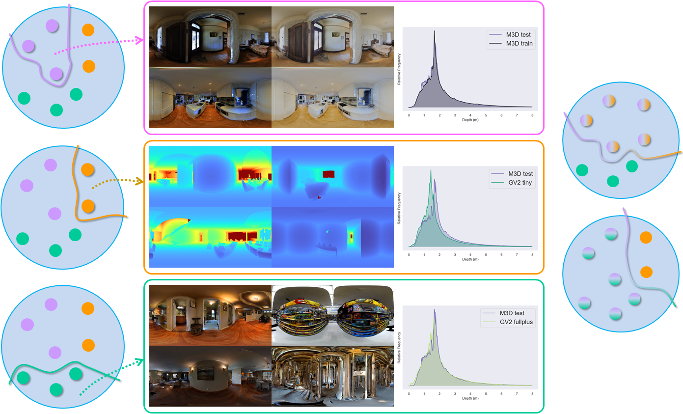
A covariate distribution shift represents a shift of the input domain, which in our case is the color image’s domain. As we rely on a synthesis approach (i.e. raytracing) to generate our data, we are also in control of the camera color transfer function. Consequently, we can generate a shifted input distribution using the M3D test split , where only the color domain has been shifted.
After examining the different splits’ statistics we also observe a prior probability distribution shift manifesting at the tiny, , and medium, , splits which corresponds to , meaning that the output depth distribution has shifted from the training one . Yet, the input (color) distribution is similar as the color camera transfer function is the same, and the context is also preserved to residential scenes.
Finally, analysing the fullplus split, we observe a concept distribution shift, which is the shifted context of the depicted scenes. While Matterport3D (i.e. ) only contains indoor residential scenes, the fullplus split presents varying scenes like supermarkets, garages, under construction buildings, etc., corresponding to . At the same time though, the input (color) and output (depth) distributions are preserved between and .
Notably, our benchmark decomposes the wider domain shift into three distinct distribution shifts. But since we rely on synthesis processes, it is straightforward to combine distribution shifts, producing and by re-rendering the corresponding splits with a shifted color transfer function, essentially adding a covariant shift to the prior and concept ones. This provides two extra combined distribution shift splits, with only the simultaneous prior and concept shifts missing.
Details can be seen in Figure 3. All of our data are publicly available at: vcl3d.github.io/Pano3D.
3 Analysis
We support our benchmark with a set of zero-shot cross-dataset transfer experiments across the different distribution shifts. We use a standard UNet [15] architecture training a supervised model with a complex objective similar to [16]:
| (1) |
where is an L1 loss, is an angular loss defined on the surface normals, is the multi-scale gradient matching loss from [17], and is the virtual normal loss [18]. All the independent term weights are equally weighted, i.e. We initialize our model using [19] and optimize it using a batch size of and the Adam optimizer [20], using a learning rate of and its default momentum parameter values.
When training we only use and for all experiments we calculate standard metrics for depth estimation [21], as well as boundary [22, 23] and normals RMSE and accuracies [24]. We aggregate performance across the different traits (direct depth, boundary and smoothness) them using a set of indicators:
| (2) | ||||
| (3) | ||||
| (4) |
where and are the depth and normal angular errors respectively, is the accuracy boundary error from [22], is the F1-score for different edge thresholds from [23], and and are the accuracy under thresholds for the depth and surface normals from [21] and [24] respectively.
Through these indicators we present an holistic view of how task performance is affected from the different distribution shifts. In the following subsections, we examine isolated distribution shifts as well as some of their combinations.
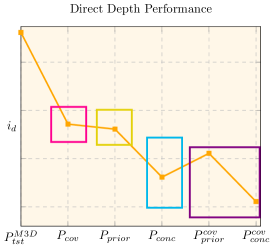
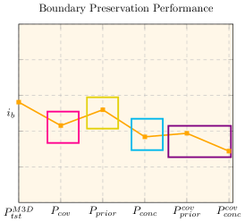
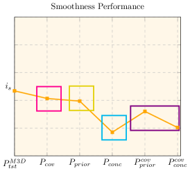
Decomposed Shifts: Varying the input, output and combined domains. After training a supervised model on M3D’s train split, we examine its performance on the different distribution shifts we have generated compared to that of the in-distribution test set. Figure 4 illustrates the results using the indicators from Eq. (2). We observe a performance drop for all distribution shifts, with the covariate (magenta box) and prior (orange box) being at about the same level, while the concept shift (cyan box) presents the largest performance loss. At the same time, combining two distribution shifts hurts performance even more, as shown by the combined distribution shifts (violet box).
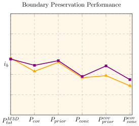
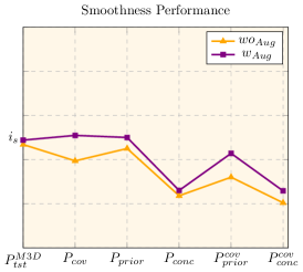
Photometric augmentations for covariate shift. Next, we examine the effect of training with photometric augmentations (i.e. brightness, contrast, hue shifts, and gamma corrections) and testing on the different (combined or not) distribution shifts. Figure 5 presents the results comparing training with and without augmentations. It is generally acknowledged that photometric augmentations address camera domain or color transfer function shifts, and our experiments verify this, as performance gains are only observed in the splits where covariate shifts manifests.
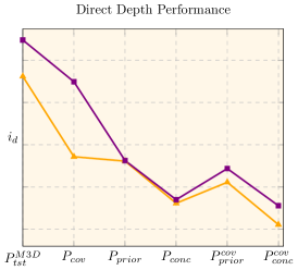
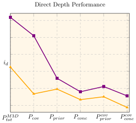
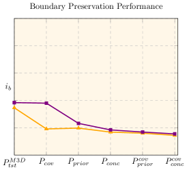
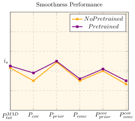
Pretraining for generalization boost. Another common assumption is that pretraining on large image datasets like ImageNet [25] helps address domain shifts. We perform another experiment, this time using the PNAS model [26] with all hyperparameters preserved, and train one model initialized with pretrained weights and another one initialized using [19]. Figure 6 presents the results when tested on our benchmark’s different shifts. Interestingly, we observe a performance boost in the splits where only a single distribution shift is present, where in contrast, the ones with two stacked distribution shifts show minimal gains. This indicates that pretraining does not necessarily improve generalization – in the form of more transferable initial features – but, instead, only provides a better parameter initialization leading to higher quality parameters’ optimization.
The full array of the conducted experiments and their detailed results can be found in Table 1.
4 Conclusion
Distribution shifting is pivotal to the real-world application of data-driven methods. In this work, we contribute a distribution shift benchmark for an ill-posed dense computer vision task, with notoriously difficult data collection process. Seeking to facilitate future research towards addressing this challenging problem, we decompose distribution shift to input (covariate), output (prior) and their relationship (concept), providing an experimental baseline for further experimentation and understanding.
| Model | Split | Direct Depth | Depth Discontinuity | Depth Smoothness | ||||||||||||||||||
|---|---|---|---|---|---|---|---|---|---|---|---|---|---|---|---|---|---|---|---|---|---|---|
| Error | Accuracy | Error | Accuracy | Error | Accuracy | |||||||||||||||||
| RMSE | RMSLE | AbsRel | SqRel | dbeacc | dbecomp | prec | prec | prec | rec | rec | rec | RMSEo | ||||||||||
| UNet | PM3Dtst | 0.452 | 0.130 | 0.115 | 0.081 | 36.68% | 60.59% | 88.31% | 96.96% | 98.73% | 1.270 | 3.888 | 58.97% | 57.54% | 51.85% | 43.96% | 36.69% | 28.59% | 16.021 | 61.80% | 76.58% | 81.70% |
| Pcov | 0.546 | 0.130 | 0.135 | 0.113 | 29.08% | 52.44% | 83.47% | 83.68% | 95.28% | 1.526 | 4.404 | 63.64% | 63.33% | 57.23% | 36.15% | 29.03% | 20.73% | 17.398 | 59.82% | 75.62% | 81.10% | |
| Pprior | 0.472 | 0.206 | 0.173 | 0.141 | 21.85% | 41.67% | 81.49% | 81.62% | 95.73% | 1.473 | 4.338 | 61.43% | 64.51% | 60.21% | 46.53% | 40.67% | 33.08% | 17.357 | 57.01% | 74.59% | 80.71% | |
| Pconc | 0.617 | 0.266 | 0.184 | 0.193 | 23.41% | 42.42% | 76.21% | 76.44% | 92.30% | 1.723 | 5.037 | 54.45% | 56.37% | 52.31% | 34.61% | 29.07% | 23.02% | 22.059 | 46.84% | 66.09% | 73.41% | |
| Pcovprior | 0.545 | 0.232 | 0.185 | 0.185 | 22.82% | 42.82% | 79.43% | 79.58% | 93.73% | 1.694 | 4.844 | 57.63% | 59.49% | 53.19% | 37.47% | 31.28% | 23.22% | 19.219 | 53.24% | 71.44% | 78.00% | |
| Pcovconc | 0.737 | 0.297 | 0.220 | 0.411 | 20.96% | 38.47% | 70.20% | 70.46% | 87.99% | 1.948 | 5.560 | 50.65% | 50.90% | 44.46% | 26.76% | 21.28% | 15.46% | 23.898 | 43.54% | 63.06% | 70.69% | |
| UNetaug | PM3Dtst | 0.433 | 0.068 | 0.109 | 0.073 | 37.36% | 63.11% | 89.59% | 89.76% | 97.42% | 1.360 | 3.876 | 64.82% | 64.94% | 60.41% | 44.96% | 37.02% | 27.96% | 15.099 | 63.99% | 77.98% | 82.83% |
| Pcov | 0.469 | 0.073 | 0.117 | 0.091 | 35.35% | 61.31% | 88.20% | 88.40% | 96.83% | 1.443 | 4.156 | 64.27% | 63.79% | 58.79% | 42.17% | 34.00% | 25.21% | 15.653 | 63.92% | 78.34% | 83.34% | |
| Pprior | 0.458 | 0.084 | 0.170 | 0.102 | 20.43% | 39.73% | 81.19% | 81.32% | 96.19% | 1.448 | 4.268 | 62.69% | 66.19% | 62.27% | 47.56% | 41.51% | 32.90% | 16.307 | 59.48% | 76.41% | 82.16% | |
| Pconc | 0.601 | 0.103 | 0.176 | 0.152 | 23.61% | 42.70% | 76.98% | 77.22% | 92.78% | 1.704 | 5.006 | 56.24% | 58.18% | 53.33% | 35.45% | 29.78% | 23.07% | 20.870 | 49.29% | 68.06% | 75.09% | |
| Pcovprior | 0.475 | 0.087 | 0.174 | 0.114 | 20.22% | 39.51% | 80.39% | 80.52% | 95.70% | 1.533 | 4.392 | 60.69% | 63.32% | 59.43% | 44.54% | 38.01% | 29.63% | 16.669 | 58.74% | 75.78% | 81.62% | |
| Pcovconc | 0.624 | 0.108 | 0.183 | 0.170 | 22.78% | 41.57% | 75.56% | 75.80% | 92.06% | 1.769 | 5.148 | 54.64% | 55.56% | 50.02% | 32.85% | 26.91% | 20.50% | 21.234 | 48.58% | 67.49% | 74.58% | |
| Pnas | PM3Dtst | 0.561 | 0.085 | 0.133 | 0.120 | 32.69% | 56.94% | 96.30% | 95.38% | 97.95% | 2.654 | 5.730 | 38.73% | 30.26% | 23.58% | 18.74% | 10.48% | 8.48% | 20.118 | 53.88% | 69.81% | 75.65% |
| Pcov | 0.703 | 0.109 | 0.160 | 0.159 | 23.45% | 45.12% | 76.27% | 77.79% | 92.06% | 2.869 | 6.075 | 36.70% | 28.00% | 18.99% | 12.33% | 6.80% | 5.32% | 21.486 | 52.07% | 68.75% | 74.91% | |
| Pprior | 0.562 | 0.098 | 0.188 | 0.146 | 19.67% | 38.39% | 76.37% | 77.53% | 94.28% | 2.651 | 5.243 | 34.12% | 29.20% | 23.15% | 18.43% | 11.70% | 9.68% | 19.929 | 52.64% | 70.83% | 77.51% | |
| Pconc | 0.693 | 0.117 | 0.200 | 0.196 | 21.27% | 39.37% | 72.84% | 73.10% | 90.80% | 3.192 | 7.277 | 32.20% | 25.87% | 19.51% | 13.69% | 8.32% | 6.68% | 24.433 | 44.01% | 63.45% | 71.07% | |
| Pcovprior | 0.663 | 0.116 | 0.192 | 0.170 | 21.21% | 40.24% | 74.54% | 74.72% | 91.12% | 3.266 | 7.251 | 29.89% | 24.68% | 17.70% | 11.58% | 7.01% | 5.58% | 22.493 | 47.89% | 66.76% | 73.90% | |
| Pcovconc | 0.842 | 0.145 | 0.222 | 0.244 | 18.50% | 34.75% | 65.66% | 65.93% | 85.70% | 3.674 | 7.881 | 28.13% | 21.04% | 13.40% | 8.15% | 4.65% | 3.70% | 26.583 | 39.92% | 59.69% | 67.72% | |
| Pnaspre | PM3Dtst | 0.467 | 0.070 | 0.107 | 0.086 | 40.90% | 64.98% | 90.38% | 90.56% | 97.33% | 2.217 | 5.019 | 44.35% | 37.55% | 31.57% | 25.78% | 15.54% | 11.60% | 17.785 | 59.34% | 73.58% | 78.80% |
| Pcov | 0.492 | 0.074 | 0.114 | 0.094 | 39.53% | 62.86% | 88.92% | 89.14% | 96.92% | 2.304 | 6.118 | 44.83% | 37.46% | 31.06% | 24.20% | 14.55% | 10.87% | 18.066 | 60.24% | 74.64% | 79.93% | |
| Pprior | 0.501 | 0.087 | 0.172 | 0.112 | 18.89% | 37.30% | 80.83% | 80.99% | 96.34% | 2.307 | 5.936 | 40.62% | 37.67% | 34.14% | 26.48% | 18.37% | 14.72% | 18.003 | 57.90% | 74.54% | 80.52% | |
| Pconc | 0.616 | 0.103 | 0.174 | 0.149 | 23.20% | 41.88% | 77.59% | 77.87% | 93.24% | 2.658 | 6.712 | 38.10% | 32.81% | 27.60% | 20.23% | 13.14% | 10.46% | 22.060 | 49.32% | 67.63% | 74.63% | |
| Pcovprior | 0.531 | 0.093 | 0.189 | 0.130 | 16.68% | 32.96% | 78.06% | 78.21% | 95.67% | 2.400 | 6.094 | 39.70% | 36.16% | 32.07% | 24.74% | 16.74% | 13.23% | 17.949 | 58.22% | 74.70% | 80.59% | |
| Pcovconc | 0.649 | 0.109 | 0.184 | 0.161 | 21.98% | 39.44% | 75.48% | 75.77% | 92.34% | 2.790 | 6.918 | 37.29% | 31.64% | 25.48% | 18.25% | 11.48% | 9.10% | 22.019 | 49.63% | 67.78% | 74.69% | |
Acknowledgments and Disclosure of Funding
This work was supported by the EC funded H2020 project ATLANTIS [GA 951900].
References
- [1] Joaquin Quiñonero-Candela, Masashi Sugiyama, Neil D Lawrence, and Anton Schwaighofer. Dataset shift in machine learning. Mit Press, 2009.
- [2] Karin Stacke, Gabriel Eilertsen, Jonas Unger, and Claes Lundström. A closer look at domain shift for deep learning in histopathology. In COMPAY19: 2nd MICCAI workshop on Computational Pathology, Shenzhen, China, October 13 2019, 2019.
- [3] Abhimanyu Dubey, Vignesh Ramanathan, Alex Pentland, and Dhruv Mahajan. Adaptive methods for real-world domain generalization. In Proceedings of the IEEE/CVF Conference on Computer Vision and Pattern Recognition, pages 14340–14349, 2021.
- [4] Mingtian Zhang, Andi Zhang, and Steven McDonagh. On the out-of-distribution generalization of probabilistic image modelling. In Thirty-Fifth Conference on Neural Information Processing Systems, 2021.
- [5] Anders Andreassen, Yasaman Bahri, Behnam Neyshabur, and Rebecca Roelofs. The evolution of out-of-distribution robustness throughout fine-tuning. arXiv preprint arXiv:2106.15831, 2021.
- [6] Ali Geisa, Ronak Mehta, Hayden S Helm, Jayanta Dey, Eric Eaton, Carey E Priebe, and Joshua T Vogelstein. Towards a theory of out-of-distribution learning. arXiv preprint arXiv:2109.14501, 2021.
- [7] Zheyan Shen, Jiashuo Liu, Yue He, Xingxuan Zhang, Renzhe Xu, Han Yu, and Peng Cui. Towards out-of-distribution generalization: A survey. arXiv preprint arXiv:2108.13624, 2021.
- [8] Jingkang Yang, Kaiyang Zhou, Yixuan Li, and Ziwei Liu. Generalized out-of-distribution detection: A survey. arXiv preprint arXiv:2110.11334, 2021.
- [9] Pang Wei Koh, Shiori Sagawa, Sang Michael Xie, Marvin Zhang, Akshay Balsubramani, Weihua Hu, Michihiro Yasunaga, Richard Lanas Phillips, Irena Gao, Tony Lee, et al. Wilds: A benchmark of in-the-wild distribution shifts. In International Conference on Machine Learning, pages 5637–5664. PMLR, 2021.
- [10] Angel Chang, Angela Dai, Thomas Funkhouser, Maciej Halber, Matthias Niebner, Manolis Savva, Shuran Song, Andy Zeng, and Yinda Zhang. Matterport3d: Learning from rgb-d data in indoor environments. In 2017 International Conference on 3D Vision (3DV), pages 667–676. IEEE Computer Society, 2017.
- [11] Fei Xia, William B Shen, Chengshu Li, Priya Kasimbeg, Micael Edmond Tchapmi, Alexander Toshev, Roberto Martín-Martín, and Silvio Savarese. Interactive gibson benchmark: A benchmark for interactive navigation in cluttered environments. IEEE Robotics and Automation Letters, 5(2):713–720, 2020.
- [12] Rui Hu, Jitao Sang, Jinqiang Wang, and Chaoquan Jiang. Understanding and testing generalization of deep networks on out-of-distribution data. arXiv preprint arXiv:2111.09190, 2021.
- [13] Marco Federici, Ryota Tomioka, and Patrick Forré. An information-theoretic approach to distribution shifts. arXiv preprint arXiv:2106.03783, 2021.
- [14] Olivia Wiles, Sven Gowal, Florian Stimberg, Sylvestre Alvise-Rebuffi, Ira Ktena, Taylan Cemgil, et al. A fine-grained analysis on distribution shift. arXiv preprint arXiv:2110.11328, 2021.
- [15] Olaf Ronneberger, Philipp Fischer, and Thomas Brox. U-net: Convolutional networks for biomedical image segmentation. In International Conference on Medical image computing and computer-assisted intervention, pages 234–241. Springer, 2015.
- [16] Georgios Albanis, Nikolaos Zioulis, Petros Drakoulis, Vasileios Gkitsas, Vladimiros Sterzentsenko, Federico Alvarez, Dimitrios Zarpalas, and Petros Daras. Pano3d: A holistic benchmark and a solid baseline for 360deg depth estimation. In Proceedings of the IEEE/CVF Conference on Computer Vision and Pattern Recognition, pages 3727–3737, 2021.
- [17] Rene Ranftl, Katrin Lasinger, David Hafner, Konrad Schindler, and Vladlen Koltun. Towards robust monocular depth estimation: Mixing datasets for zero-shot cross-dataset transfer. IEEE Transactions on Pattern Analysis and Machine Intelligence, 2020.
- [18] Wei Yin, Yifan Liu, Chunhua Shen, and Youliang Yan. Enforcing geometric constraints of virtual normal for depth prediction. In Proceedings of the IEEE/CVF International Conference on Computer Vision, pages 5684–5693, 2019.
- [19] Kaiming He, Xiangyu Zhang, Shaoqing Ren, and Jian Sun. Delving deep into rectifiers: Surpassing human-level performance on imagenet classification. In Proceedings of the IEEE international conference on computer vision, pages 1026–1034, 2015.
- [20] Diederik P Kingma and Jimmy Ba. Adam: A method for stochastic optimization. arXiv preprint arXiv:1412.6980, 2014.
- [21] David Eigen, Christian Puhrsch, and Rob Fergus. Depth map prediction from a single image using a multi-scale deep network. Advances in Neural Information Processing Systems, 27:2366–2374, 2014.
- [22] Tobias Koch, Lukas Liebel, Friedrich Fraundorfer, and Marco Korner. Evaluation of cnn-based single-image depth estimation methods. In Proceedings of the European Conference on Computer Vision (ECCV) Workshops, pages 0–0, 2018.
- [23] Junjie Hu, Mete Ozay, Yan Zhang, and Takayuki Okatani. Revisiting single image depth estimation: Toward higher resolution maps with accurate object boundaries. In 2019 IEEE Winter Conference on Applications of Computer Vision (WACV), pages 1043–1051. IEEE, 2019.
- [24] Rui Wang, David Geraghty, Kevin Matzen, Richard Szeliski, and Jan-Michael Frahm. Vplnet: Deep single view normal estimation with vanishing points and lines. In Proceedings of the IEEE/CVF Conference on Computer Vision and Pattern Recognition, pages 689–698, 2020.
- [25] Jia Deng, Wei Dong, Richard Socher, Li-Jia Li, Kai Li, and Li Fei-Fei. Imagenet: A large-scale hierarchical image database. In 2009 IEEE conference on computer vision and pattern recognition, pages 248–255. Ieee, 2009.
- [26] Chenxi Liu, Barret Zoph, Maxim Neumann, Jonathon Shlens, Wei Hua, Li-Jia Li, Li Fei-Fei, Alan Yuille, Jonathan Huang, and Kevin Murphy. Progressive neural architecture search. In Proceedings of the European conference on computer vision (ECCV), pages 19–34, 2018.