AR-sieve Bootstrap for High-dimensional Time Series

Abstract

This paper proposes a new AR-sieve bootstrap approach on high-dimensional time series. The major challenge of classical bootstrap methods on high-dimensional time series is two-fold: the curse dimensionality and temporal dependence. To tackle such difficulty, we utilise factor modelling to reduce dimension and capture temporal dependence simultaneously. A factor-based bootstrap procedure is constructed, which conducts AR-sieve bootstrap on the extracted low-dimensional common factor time series and then recovers the bootstrap samples for original data from the factor model. Asymptotic properties for bootstrap mean statistics and extreme eigenvalues are established. Various simulations further demonstrate the advantages of the new AR-sieve bootstrap under high-dimensional scenarios. Finally, an empirical application on particulate matter (PM) concentration data is studied, where bootstrap confidence intervals for mean vectors and autocovariance matrices are provided.

Keywords: Autocovariance matrices; Factor models; High-dimensional time series; AR-sieve bootstrap; Temporal dependence

1 Introduction

The bootstrap is a computer-intensive resampling-based methodology that arises as an alternative to asymptotic theory. The bootstrap method, initially introduced by Efron (1979) for independent sample observations, is later extended to more complicated dependent data in the literature. As an important extension to stationary time series, blockwise bootstrap (Künsch, 1989), autoregressive (AR) sieve bootstrap (Kreiss, 1988; Bühlmann, 1997), and frequency-domain bootstrap (Franke & Hardle, 1992; Dahlhaus & Janas, 1996) have received the most discussions and developments in the past few years. A few variants of block bootstrap methods have appeared, such as the block bootstrap for time series with fixed regressors (Nordman & Lahiri, 2012), the double block bootstrap (Lee & Lai, 2009), and the stationary bootstrap (Politis & Romano, 1994), among others. An apparent disadvantage of blockwise bootstrap is neglected dependence between different blocks. The AR-sieve bootstrap method takes up the “sieve” strategy, which approximates stationary time series by an AR model with a large number of time lags. Compared with the blockwise bootstrap, the AR-sieve bootstrap samples are conditionally stationary and keep the dependence structure well. The AR-sieve bootstrap is introduced by Kreiss (1988) and has been well studied from stationary linear processes (Bühlmann, 1997) to strictly stationary time series fulfilling a general moving average MA ($\infty$) representation (Kreiss et al., 2011). After this work, the theoretical requirement and validity of a general AR-sieve bootstrap method for certain type of statistics have been discussed for univariate (Kreiss et al., 2011), multivariate (Meyer & Kreiss, 2015) and functional time series (Paparoditis, 2018; Paparoditis & Shang, 2021), respectively. The frequency-domain bootstrap to implement the resampling schemes is based on frequency-domain methods. The motivation behind this method comes from the observation that periodogram ordinates at a finite number of frequencies are approximately independent distributed so that Efron’s ideas may be employed. Compared to the AR-sieve bootstrap, this method could deal with more general dependence structures for time series (Meyer et al., 2020; Hidalgo, 2021).

The main goal of this paper is to extend the AR-sieve bootstrap to high-dimensional time series. Due to the curse of dimensionality, traditional AR-sieve bootstrap fails in the high-dimensional case. This is because the AR model approximation for high-dimensional time series could result in a large approximation error, and the bootstrap procedure on high-dimensional i.i.d residual is also inaccurate. The curse of dimensionality on traditional bootstrap methods is demonstrated vividly in El Karoui & Purdom (2018). As a remedy, reducing the parameter space is essential for successful modifying bootstrap methods. Fitting sparse models and low-rank models to high-dimensional data are two commonly used techniques to eliminate the curse of dimensionality. Chernozhukov et al. (2017) provide theoretical guarantee on the bootstrap approximation for the distribution of the sample mean vector for high-dimensional i.i.d data. Chen (2018) studies the bootstrap approximation for U-statistics constructed by high-dimensional i.i.d data. Ahn & Reinsel (1988) propose a nested reduce-rank structure for coefficients in multivariate AR time series model. For high-dimensional time series, Krampe et al. (2021) consider AR-sieve bootstrap for vector AR time series with sparse coefficients. In this article, we will contribute to proposing an appropriate low-rank model for AR-sieve bootstrap on high-dimensional stationary time series.

Factor modelling or low-rank representation can project high-dimensional data into low-dimensional subspace. Principal component analysis (PCA) is a common technique to pursue projections or subspace with the most variation in the original data (Bai & Ng, 2002; Fan et al., 2011). Identifying the low-dimensional representation for high-dimensional time series is more complicated because keeping the temporal dependence in dimension reduction is a crucial requirement. Earlier literature of this field on multivariate time series is vast and includes the canonical correlation analysis (Box & Tiao, 1977), the factor models (Pena & Box, 1987), and the scalar component model (Tiao & Tsay, 1989). Later Lam et al. (2011) study a factor model for high-dimensional time series based on an accumulation of autocovariance matrices, aiming to capture all temporal dependence by common factors.

In this article, we reduce high-dimensional time series based on a factor model whose common factors possess all temporal dependence of the original time series. Efficient estimation for such factor model is borrowed from the idea of Lam et al. (2011), which conduct eigendecomposition for a set of autocovariance matrices with various time-lags. With the lower-dimensional common factors time series, the AR-sieve bootstrap is feasible and produces bootstrap samples for common factors. Finally, the AR-sieve bootstrap could recover the relationship between common factors and the original high-dimensional time series.

We also study the theoretical properties of the proposed AR-sieve bootstrap on two commonly used statistics - the mean statistics and spectral statistics of autocovariance matrices. Common factors stand at a “representation and activation” position in the whole bootstrap method. Under the scenario of comparable $N$ (the dimension) and $T$ (the time-serial length), we first provide convergence rates for the estimation of common factors, which could affect statistical properties of the final AR-sieve bootstrap statistics. Further, for the two high-dimensional statistics under consideration, the consistency of the bootstrap versions to the population versions is established. Finite-sample experiments demonstrate the influences of the dimension, the sample size and factors’ strength on the bootstrap results. Moreover, we also conduct an empirical application on $\text{PM}_{10}$ data. As a by-product of interest, we apply the proposed AR-sieve bootstrap for high-dimensional series on sparsely-observed discrete functional time series and compare them with the results from AR-sieve bootstrap for functional time series (Paparoditis, 2018). Due to the smoothing inaccuracy for sparsely-observed discrete functional time series, the high-dimensional bootstrap method sometimes results in better statistical inferences than the functional approach by smoothing them. Various simulations in the appendix could reflect this point.

The rest of this paper is organised as follows. Section 2 introduces factor models for high-dimensional time series and discusses the AR representation of the factor time series, a building block of the general AR-sieve bootstrap. In Section 3, the estimation procedure for factor models and the AR-sieve bootstrap procedure for factor time series is introduced with regularity conditions on factor models. The additional assumptions and asymptotic validity of our novel AR-sieve bootstrap method are discussed in Section 4. Mean statistics of factor time series and spiked eigenvalues of symmetrised autocovariance matrices are introduced. In Section 5, via several simulation experiments, we verify the validity of our novel AR-sieve bootstrap methods on the mean statistics and the spiked eigenvalues of symmetrised autocovariance matrices. Section 6 provides an example of applying our novel AR-sieve bootstrap method to $\text{PM}_{10}$ data. Conclusions are presented in Section 7. In the supplementary, Appendix A explores the impact of density of discrete functional time-series observations on pre-smoothing results. Technical proofs and auxiliary lemmas are presented in Appendices B and C in additional supplementary documents.

2 Factor-based AR-sieve Representation

In this section, we first propose a factor model to project the high-dimensional time series into a lower-dimensional subspace. Common-factors time series could represent the original data to capture the most temporal dependence. Secondly, an AR-sieve representation for common factors is provided, which plays a significant role in the AR-sieve bootstrap.

Consider a stationary $N$-dimensional time series $\{\bm{y}_{t}\in\mathbb{R}^{N},\ t\in\mathbb{Z}\}$ following a general unobservable factor model

$$\bm{y}_{t}=\bm{Q}\bm{f}_{t}+\bm{u}_{t},\ \ \ t=1,2,\ldots,T,$$ (1)

where $\{\bm{f}_{t}\in\mathbb{R}^{r},\ t\in\mathbb{Z}\}$ are unobserved $r$-dimensional factor time series, $\bm{Q}$ is an $N\times r$ factor loading matrix and $\{\bm{u}_{t}\in\mathbb{R}^{r},\ t\in\mathbb{Z}\}$ are $N$-dimensional white noises with zero means and covariance matrix $\bm{\Sigma}_{u}$.

Factor models have received numerous discussions, and there are various identification conditions and assumptions on $\bm{Q}$, $\bm{f}_{t}$ and $\bm{u}_{t}$ depending on various aims. In our work, we adapt the identification condition in Lam et al. (2011) to consider a factor model where temporal dependence of $\{\bm{y}_{t}\}$ can be fully captured by the factors $\{\bm{f}_{t}\}$. It is noteworthy that we do not require a direct dynamic system on $\{\bm{f}_{t}\}$. Therefore we still maintain a static relationship between $\{\bm{y}_{t}\}$ and $\{\bm{f}_{t}\}$.

Next, we introduce an AR-sieve representation for multivariate common-factors time series. For the $r\times 1$ common factors $\{\bm{f}_{t}\}$, we know via Wold’s theorem (see, e.g., Bühlmann, 1997) that $\{\bm{f}_{t}\}$ can be written as a one-sided infinite-order moving-average (MA) process

$$\bm{f}_{t}=\sum_{l=1}^{\infty}\bm{\Psi}_{l}\bm{e}_{t-l}+\bm{e}_{t},\ t\in\mathbb{Z},$$ (2)

where $\{\bm{e}_{t}\in\mathbb{R}^{r},\ t\in\mathbb{Z}\}$ are full rank uncorrelated white-noise innovation processes with $\mathbb{E}(\bm{e}_{t})=0$ and $\mathbb{E}(\bm{e}_{t}\bm{e}_{s}^{\top})=\mathbf{1}_{t=s}\bm{\Sigma}_{e}$, with $\bm{\Sigma}_{e}$ a full rank $r\times r$ covariance matrix. $\{\bm{\Psi}_{l}\in\mathbb{R}^{r\times r},\ l\in\mathbb{N}\}$ are the coefficients matrices.

Under the requirement on invertibility of the process in (2), which would narrow the class of stationary processes a little bit, we can represent $\{\bm{f}_{t}\}$ as a one-sided infinite-order autoregressive (AR) process. That is, there exists an infinite sequence of $r\times r$ matrices $\{\bm{A}_{l}\in\mathbb{R}^{r\times r},\ l\in\mathbb{N}\}$ such that factors $\{\bm{f}_{t}\}$ can be expressed as

$$\bm{f}_{t}=\sum_{l=1}^{\infty}\bm{A}_{l}\bm{f}_{t-l}+\bm{e}_{t},\ t\in\mathbb{Z},$$ (3)

where the coefficient matrices of the expansion for the power series $\left(\bm{I}_{r}-\sum_{l=1}^{\infty}\bm{A}_{l}z^{l}\right)^{-1}$ are $\{\bm{\Psi}_{l}\in\mathbb{R}^{r\times r},\ l\in\mathbb{N}\}$. Here $|z|\leq 1$ (Brockwell & Davis, 1991). Note that (2) is a representation instead of an imposed assumption or model. AR-sieve bootstrap is based on an approximated AR representation for (3), i.e.

$$\bm{f}_{t}\approx\sum_{l=1}^{p}\bm{A}_{l}\bm{f}_{t-l}+\bm{e}_{t},\ t\in\mathbb{Z},$$ (4)

where $p$ is a large integer that tends to infinity, in this sense, AR-sieve bootstrap is a nonparametric approach although (4) looks like a “fake“ parametric model.

The (vector) AR representation in (3) is more attractive for statistical applications and has received more attention since it relates $\bm{f}_{t}$ to its past values. AR-sieve bootstrap, on the other hand, utilises the AR-representation in (3) to generate bootstrap common factors by resampling from the de-centred innovations. In practice, since neither the factors $\{\bm{f}_{t}\}$ or their loadings $\bm{Q}$ are observable, AR-sieve bootstrap is performed on estimates of $\{\bm{f}_{t}\}$ rather than true factors. Hence, we will introduce the estimation and bootstrap procedure in the following section.

3 Factor-based AR-sieve bootstrap

In this section, we first introduce the estimation approach for the factor model in (1) and then provide the AR-sieve bootstrap procedure. Further, a flow chart is shown to summarise the whole procedure of AR-sieve bootstrap for high-dimensional time series.

3.1 Analysis on common-factors estimation

Recall that common factors $\{\bm{f}_{t}\}$ in model (3) are assumed to contain all the temporal dependence of $\{\bm{y}_{t}\}$ because the error components $\{\bm{u}_{t}\}$ have no temporal dependence. As analysed by Bathia et al. (2010) and Lam et al. (2011), the factor loading space, that is, the $r$-dimensional linear space spanned by the columns of the factor loading matrix $\bm{Q}$, denoted by $\mathcal{M}(\bm{Q})$, is uniquely defined. Further, this subspace $\mathcal{M}(\bm{Q})$ is spanned by the eigenvectors of an accumulated symmetrised autocovariance matrices below, corresponding to its nonzero eigenvalues,

$$\bm{L}=\sum_{k=1}^{k_{0}}\bm{\Gamma}_{y}(k)\bm{\Gamma}_{y}(k)^{\top},$$

where $\bm{\Gamma}_{y}(k)=\text{Cov}(\bm{y}_{t},\bm{y}_{t+k})$ is the autocovariance of $\{\bm{y}_{t}\}$ at lag $k$, for $k=1,2,...,k_{0}$. Intuitively speaking, the matrix $\bm{L}$ collects the temporal dependence of $\{\bm{y}_{t}\}$ by pooling up the information contained in first $k_{0}$-lags of autocovariance with the squared (symmetrised) form facilitating the spectral decomposition on $\bm{L}$.

Remark 3.1.

The reason of not to consider the covariance matrix $\bm{\Sigma}_{y}$ into $\bm{L}$ is undemanding. As discussed by Lam et al. (2011), for the factor model (1), $\bm{\Sigma}_{y}=\bm{\Gamma}_{y}(0)=\bm{Q}\bm{\Gamma}_{\bm{f}}(0)\bm{Q}^{\top}+\bm{\Sigma}_{u}$, where $\bm{\Gamma}_{\bm{f}}(0)$ is the covariance matrix of $\{\bm{y}_{t}\}$ and $\bm{\Sigma}_{u}$ is the covariance matrix of $\{\bm{u}_{t}\}$. Hence to exclude $\bm{\Sigma}_{y}$ from $\bm{L}$ can filter out the impact of covariance on $\{\bm{u}_{t}\}$, especially for $N\to\infty$.

It is then straightforward to use spectral (eigenvalue) decomposition on $\bm{L}$ to estimate the factor loading matrix $\bm{Q}$, and the factors $\{\bm{f}_{t}\}$. Before the details of the estimation procedure, we summarise the assumptions and identification conditions for the factor model defined in (1) first.

Assumptions 3.1 (Conditions on Factor models).

For factor models (1), we impose the following assumptions,

1. $\{\bm{f}_{t}\}$ are strictly stationary time series with $\mathbb{E}\bm{f}_{t}=\mathbf{0}$ and $\mathbb{E}\left\|\bm{f}_{t}\right\|^{2}<\infty$; $\{\bm{u}_{t}\}\sim WN(0,\bm{\Sigma}_{u})$ are uncorrelated white noises with covariance matrix $\bm{\Sigma}_{u}$, and all eigenvalues of $\bm{\Sigma}_{u}$ are uniformly bounded as $N\to\infty$; $\{\bm{f}_{t}\}$ are independent of $\{\bm{u}_{s}\}$ for any $t,s\in\mathbb{Z}$.

2. $\frac{1}{N}\bm{Q}^{\top}\bm{Q}=\bm{I}_{r}$ and for a prescribed integer $k_{0}>0$, the $r\times r$ matrix $\bm{\Gamma}_{f}(k)=\text{Cov}(\bm{f}_{t},\bm{f}_{t+k})$ is of full rank for any $k=0,1,...,k_{0}$, i.e. the eigenvalues $\{\lambda_{i}(\bm{f}),\ i=1,2,...,r\}$ of the matrix $\sum_{k=1}^{k_{0}}\bm{\Gamma}_{f}(k)\bm{\Gamma}_{f}(k)^{\top}$ satisfy $\infty>\lambda_{1}(\bm{f})\geq\lambda_{2}(\bm{f})\geq\cdots\geq\lambda_{r}(\bm{f})>0$ as $N\to\infty$.

3. $\{\bm{y}_{t}\}$, therefore $\{\bm{f}_{t}\}$, are $\psi$-mixing with the mixing coefficients $\psi(\cdot)$ satisfying the condition that $\sum_{t\geq 1}\psi(t)^{1/2}<\infty$, and $\mathbb{E}{|y_{j,t}|^{4}}<\infty$ element-wisely.

Next, we provide some comments and justifications on Assumption 3.1.

1. Assumption 3.1 (i) states the strict stationarity on $\{\bm{f}_{t}\}$, which has been used in literature of factor models, such as Fan et al. (2013) and is commonly seen in AR-sieve bootstrap literature, such as Kreiss et al. (2011) and Meyer & Kreiss (2015). Apart from the stationarity, Assumption 3.1 (i) also states that factor time series $\{\bm{f}_{t}\}$ and error terms $\{\bm{u}_{t}\}$ are independent at any time lags, which is stronger than the assumption in Lam et al. (2011), but is required for us to apply bootstrap methods by resampling from the innovations $\{\bm{e}_{t}\}$ in Wold representation of $\{\bm{f}_{t}\}$ as in (2), since AR-sieve bootstrap does not work for high-dimensional noises $\{\bm{u}_{t}\}$.

2. We impose Assumption 3.1 (ii) to identify the factor components $\{\bm{Q}\bm{f}_{t}\}$ from the original high-dimensional data. The conditions that $\frac{1}{N}\bm{Q}^{\top}\bm{Q}=\bm{I}_{r}$ and eigenvalues $\{\lambda_{i}(\bm{f}),\ i=1,2,...,r\}$ of $\sum_{k=1}^{k_{0}}\bm{\Gamma}_{f}(k)\bm{\Gamma}_{f}(k)^{\top}$ fulfil $\infty>\lambda_{1}(\bm{f})\geq\lambda_{2}(\bm{f})\geq\cdots\geq\lambda_{r}(\bm{f})>0$ as $N\to\infty$ are sufficient for $\{\bm{Q}\bm{f}_{t}\}$ to be identifiable from $\{\bm{u}_{t}\}$ when $N\to\infty$, since the $N\times N$ matrix $\bm{L}$ can be represented as

   $$\bm{L}=\sum_{k=1}^{k_{0}}\bm{\Gamma}_{y}(k)\bm{\Gamma}_{y}(k)^{\top}=N\bm{Q}\left\{\sum_{k=1}^{k_{0}}\bm{\Gamma}_{\bm{f}}(k)\bm{\Gamma}_{\bm{f}}(k)^{\top}\right\}\bm{Q}^{\top},$$ (5)

   with the first $r$ eigenvalues of $\frac{1}{N^{2}}\bm{L}$ non-vanishing. In other words, the columns of $\bm{Q}$ can be considered as the eigenvectors of $\bm{L}$ corresponding to $r$ nonzero eigenvalues scaled by $\sqrt{N}$. As a consequence, Assumption 3.1 (ii) implies the pervasiveness of $r$ factors $\{\bm{f}_{t}\}$ when $N$ goes to infinity, which is equivalent to the strong factors’ case according to the definition in Lam et al. (2011).

3. The $\psi$-mixing in Assumption 3.1 (iii) is introduced to specify the week dependence structure of $\{\bm{f}_{t}\}$, which is considered in Lam et al. (2011) to simplify the technical proof of consistency on loading matrix $\bm{Q}$. However, it is not the weakest possible. In the meantime, Assumption 3.1 (ii) together with the mixing condition in (iii) is also sufficient for the absolute summability condition on $\{\bm{f}_{t}\}$ when $N\to\infty$, which is preliminary for AR-sieve bootstrap to be applicable on $\{\bm{f}_{t}\}$, since otherwise the Wold representation is not guaranteed to exist (Cheng & Pourahmadi, 1993).

To further explain the use of Assumption 3.1 with the estimation procedure, first notice that $\{\bm{f}_{t}\}$ are strong factors and no linear combinations of the components of $\{\bm{f}_{t}\}$ are white noises (WN) as implied by Assumption 3.1 (ii). Recall that $\bm{L}$ is non-negative definite and can be represented as in (5) with $\frac{1}{N}\bm{Q}^{\top}\bm{Q}=\bm{I}_{r}$. Since $\sum_{k=1}^{k_{0}}\bm{\Gamma}_{\bm{f}}(k)\bm{\Gamma}_{\bm{f}}(k)^{\top}$, the middle part of (5), is symmetric, we can apply spectral decomposition on it and recognise $\bm{L}$ as $N\bm{Q}\left(\bm{S}\bm{D}\bm{S}^{\top}\right)\bm{Q}^{\top}$, where $\bm{S}$ is an $r\times r$ orthonormal matrix and $\bm{D}$ is an $r\times r$ diagonal matrix. Furthermore, since $\frac{1}{N}(\bm{Q}\bm{S})^{\top}(\bm{Q}\bm{S})=\bm{I}_{r}$, the columns of $\bm{Q}\bm{S}$ are in fact the eigenvectors of $\bm{L}$ corresponding to those non-zero eigenvalues scaled by $\sqrt{N}$. Therefore, we can treat $\bm{Q}\bm{S}$ as $\bm{Q}$ for inferences’ purpose and estimate $\bm{Q}$ and $\bm{f}_{t}$ based on the spectral decomposition of $\bm{L}$.

With regular conditions in Assumptions 3.1, we can estimate the factors and their loadings, and then generate a sample of time series with AR-sieve bootstrap. To facilitate the estimation process, we define $\bm{Q}^{o}=\frac{1}{\sqrt{N}}\bm{Q}$ as the (unscaled) orthonormal factor loading matrix such that $\bm{Q}^{o\top}\bm{Q}^{o}=\bm{I}_{r}$ and $\bm{f}^{o}_{t}$ as the scaled factors such that $\bm{y}_{t}=\bm{Q}^{o}\bm{f}^{o}_{t}+\bm{u}_{t}$ is equivalent to model (1) with different scaling on $\bm{Q}$ and $\{\bm{f}_{t}\}$. Details of the proposed method, including the estimation and the bootstrap procedure, are illustrated in the following subsection.

3.2 The procedure of factor-based AR-sieve bootstrap

In this part, we present the whole procedure for the proposed factor-based AR-sieve bootstrap. Then, a flow chart is provided to clarify the essential idea of this procedure further.

Below we divide the proposed method into four steps.

1. Step 1: Estimation of $\bm{Q}$: To utilise the idea in Lam et al. (2011) to estimate $\bm{Q}$ and $\{\bm{f}_{t}\}$ using $\bm{L}$, the accumulated symmetrised autocovariance matrices of $\{\bm{y}_{t}\}$ up to a prescribed lag $k_{0}>0$, we first define the accumulation of symmetrised sample autocovariance up to lag $k_{0}$ as

   $$\widetilde{\bm{L}}=\sum_{k=1}^{k_{0}}\bm{\widetilde{\Gamma}}_{y}(k)\bm{\widetilde{\Gamma}}_{y}(k)^{\top},$$

   with $\bm{\widetilde{\Gamma}}_{y}(k)$ the sample autocovariance at lag $k$ defined as

   $$\bm{\widetilde{\Gamma}}_{y}(k)=\frac{1}{T-k}\sum_{t=1}^{T-k}(\bm{y}_{t+k}-\overline{\bm{y}})(\bm{y}_{t}-\overline{\bm{y}})^{\top}.$$

   By applying spectral (eigenvalue) decomposition on $\widetilde{\bm{L}}$, we can obtain $\widehat{\bm{Q}^{o}}=(\widehat{\bm{q}^{o}_{1}},\widehat{\bm{q}^{o}_{2}},...,\widehat{\bm{q}^{o}_{r}})$ with $\widehat{\bm{q}^{o}_{i}}$ the eigenvector of $\widetilde{\bm{L}}$ corresponding to the $i$^th largest eigenvalue of $\widetilde{\bm{L}}$. $\widehat{\bm{Q}^{o}}$ is then a natural estimator of the unscaled loading matrix $\bm{Q}^{o}$. And by scaling up $\widehat{\bm{Q}^{o}}$ with $\sqrt{N}$, the square root of dimension, we ended up with $\bm{\widehat{Q}}=\sqrt{N}\widehat{\bm{Q}^{o}}$ as the estimator of $\bm{Q}$.

   As discussed in Lam et al. (2011), the estimation results are not sensitive to the choice of $k_{0}$, and the numeral results associated with $k_{0}=1$ to $k_{0}=5$ are similar. In general, when dimension $N$ is large compared with $T$, a relatively larger $k_{0}$ may be considered for better accuracy of sample estimates, while $k_{0}=1$ is computational more efficient when the sample size $T$ is large compared with dimension $N$. Besides, for finite samples, some of the non-spiked eigenvalues of $\widetilde{\bm{L}}$ may not be exactly zero, therefore we can use the ratio-based estimator as discussed in Lam et al. (2011) to estimate the number of factor $r$. As defined in Lam et al. (2011), the ratio-based estimator for $r$ is

   $$\widehat{r}=\operatorname*{\arg\!\min}_{1\leq j\leq R}\widehat{\lambda}_{j+1}/\widehat{\lambda}_{j},$$

   with $\widehat{\lambda}_{1}\geq\widehat{\lambda}_{2}\geq\cdots\geq\widehat{\lambda}_{N}$ the eigenvalues of $\widetilde{\bm{L}}$ and $R$ an integer satisfying $r\leq R<N$. And practically, $R$ can be taken as $N/2$ or $N/3$ for computation efficiency (Lam et al., 2011).

2. Step 2: Estimation of $\{\bm{f}_{t}\}$:

   With $\widehat{\bm{Q}}$ the estimator of $\bm{Q}$, it is then straightforward to estimate $\{\bm{f}_{t}\}$ by

   $$\widehat{\bm{f}_{t}}=\widehat{\bm{Q}}^{\top}\bm{y}_{t}.$$

3. Step 3: AR-sieve bootstrap on $\{\bm{\widehat{f}}_{t}\}$:

   To apply the AR-sieve bootstrap on $\{\bm{\widehat{f}}_{t}\}$, we can, first of all, fit a $p$^th order VAR model on the $r$-dimensional time series $\{\bm{\widehat{f}}_{t}\}$ as

   $$\bm{\widehat{f}}_{t}=\sum_{l=1}^{p}\bm{\widehat{A}}_{l,p}(r)\bm{\widehat{f}}_{t-l}+\bm{\widehat{e}}_{t,p},\ t=p+1,p+2,...,T,$$

   where $\bm{\widehat{e}}_{t,p}$ denote the residuals and the order $p$ of the VAR model can be selected based on an information criterion such as AIC (Akaike, 1974) and SC (Schwarz, 1978). Equivalently, we have

   $$\bm{\widehat{e}}_{t,p}=\bm{\widehat{f}}_{t}-\sum_{l=1}^{p}\bm{\widehat{A}}_{l,p}(r)\bm{\widehat{f}}_{t-l},\ t=p+1,p+2,...,T,$$

   where $\{\bm{\widehat{A}}_{l,p},\ l=1,2,...,p;\ t=p+1,p+2,...,T\}$ are Yule-Walker estimators of the AR coefficient matrices. We can then generate $\{\bm{e}^{\ast}_{t}\}$ the bootstrap sample of residuals by resampling from the empirical distribution of the centered residual vectors. Consequently, based on the idea of AR-sieve bootstrap (see, e.g. Kreiss, 1992; Meyer & Kreiss, 2015; Paparoditis, 2018), we can generate the $r$-dimensional pseudo-time series $\{\bm{f}_{t}^{\ast},\ t=1,2,...,T\}$ by simulating the VAR model with bootstrap residuals $\{\bm{e}^{\ast}_{t}\}$. Therefore, an AR-sieve bootstrap sample of $\{\bm{f}_{t}^{\ast}\}$ is generated by

   $$\bm{f}_{t}^{\ast}=\sum_{l=1}^{p}\bm{\widehat{A}}_{l,p}(r)\bm{f}_{t-l}^{\ast}+\bm{e}_{t}^{\ast},$$

   where $\{\bm{e}_{t}^{\ast}\}$ are i.i.d. random vectors following the empirical distribution of the centered residual vectors $\{\widetilde{\bm{e}}_{t}\}$, where $\widetilde{\bm{e}}_{t,p}=\bm{\widehat{e}}_{t,p}-\overline{\bm{\widehat{e}}}_{T,p}$ and $\overline{\bm{\widehat{e}}}_{T,p}=1/(T-p)\sum_{t=p+1}^{T}\bm{\widehat{e}}_{t,p}$.

4. Step 4: Generating bootstrap data $\{\bm{y}^{\ast}_{t}\}$:

   Lastly, the bootstrap time series $\{\bm{y}_{t}^{\ast}\}$ can be constructed as

   $$\bm{y}_{t}^{\ast}=\sum_{j=1}^{r}\bm{f}_{j,t}^{\ast}\widehat{\bm{q}_{j}},$$ (6)

   where $\widehat{\bm{q}_{j}}=\sqrt{N}\widehat{\bm{q}^{o}_{j}}$ is the scaled eigenvector of $\widehat{\bm{L}}$ corresponding to the $j$^th largest eigenvalue. Following this AR-sieve bootstrap procedure, the pseudo-time series $\{\bm{y}^{\ast}_{t}\}$ can mimic the temporal dependence of the original data $\{\bm{y}_{t}\}$ via a factor model.

Remark 3.2.

It is noteworthy that the bootstrap version in (6) is constructed via the bootstrap version of the common factors. We could also modify it to involve an additional term related to the error components. For instance, with the estimated $\bm{\widehat{u}}_{t}=\bm{y}_{t}-\bm{\widehat{Q}}\bm{\widehat{f}}_{t}$, under some regular sparse conditions on the population covariance matrix $\bm{\Sigma}_{u}$, we can get an appropriate estimator $\widehat{\Sigma}_{u}$ (Fan et al., 2013). Then a modified bootstrap version is

$$\bm{y}_{t}^{\ast\ast}=\sum_{j=1}^{r}\bm{f}_{j,t}^{\ast}\widehat{\bm{q}_{j}}+\widehat{\bm{\Sigma}}_{u}^{1/2}\widetilde{\bm{u}}_{t},$$ (7)

where $\widetilde{\bm{u}}_{t}$ is $N$-dimensional random vector generated from standard normal distribution $\mathcal{N}\ (\textbf{0}_{N},\bm{I}_{N})$. In this way, the bootstrap version $\bm{y}_{t}^{\ast\ast}$ is not of low-rank. For instance, conditional on the original sample observations, the covariance matrix of $\bm{y}_{t}^{\ast\ast}$ is of full rank. Due to high-dimensionality of the error components $\{\bm{\widehat{u}}_{t}\}$, non-parametric bootstrap on error would incur curse of dimensionality again (El Karoui & Purdom, 2018).

For simplicity, we study the mean statistics and the largest eigenvalue of sample autocovariance matrices based on the bootstrap version in (6), because (6) and (7) produce bootstrap statistics with similar asymptotic properties. The major reason is based on assumptions that (1) the population mean of error components is zero and (2) the spiked eigenvalues of autocovariance matrices are assumed to tend to infinity.

To clarify the four steps mentioned above, a flow chart is provided in Figure 1, which summarises the basic logic and procedure for the proposed factor-based AR-sieve bootstrap method.

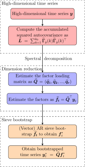
Figure 1: Flow chart for AR-sieve bootstrap method

4 Asymptotic theory

In this section, some regular assumptions and justifications are present first. Then, we establish the asymptotic properties for two commonly-used statistics: the mean statistics and the largest eigenvalues of accumulated autocovariance matrices.

4.1 Regularity assumptions

Before introducing the additional regularity assumptions, we fix some notations first. We use $\|\cdot\|_{2}$ to denote the $L_{2}$ norm (also known as spectral norm or operator norm) of a matrix or vector, and $\|\cdot\|_{F}$ to denote the Frobenius norm of a matrix. And we use $a\asymp b$ to denote the case that $a=O_{P}(b)$ and $b=O_{P}(a)$.

In addition to Assumptions 3.1 made on the factor model (1), to apply the AR-sieve bootstrap on $\{\bm{\widehat{f}}_{t}\}$, the estimates of factors $\{\bm{f}_{t}\}$, we also need some regularity conditions on $\{\bm{f}_{t}\}$ for the AR-sieve bootstrap to be consistent and valid. Denoted by $W(\cdot)$, the spectral density matrix of a vector process for all frequencies $\omega\in(0,2\pi]$, then the spectral density matrix of $\{\bm{f}_{t}\}$ can be defined as

$$W_{\bm{f}}(\omega)=\frac{1}{2\pi}\sum_{k=-\infty}^{\infty}\bm{\Gamma}_{\bm{f}}(k)e^{-i\omega k},\omega\in(0,2\pi].$$

Assumptions 4.1.

In model (1), we strengthen Assumption 3.1 such that $\{\bm{f}_{t}\}$ are strictly stationary and purely nondeterministic stochastic processes of full rank with $\mathbb{E}\bm{f}_{t}=\mathbf{0}$ and $\mathbb{E}\left\|\bm{f}_{t}\right\|^{2}<\infty$. $\bm{\Gamma}_{f}(k)$, the autocovariance matrix of $\bm{f}_{t}$ at lag $k$ fulfils the matrix norm summability condition $\sum_{k=-\infty}^{\infty}(1+|k|)^{\gamma}\left\|\bm{\Gamma}_{f}(k)\right\|_{F}<\infty$ for some $\gamma\geq 0$ that will be specified later on.

Justification for Assumption 4.1: Assumption 4.1 is introduced to fulfil the requirement for the existence of a general VAR representation (3). This type of conditions is commonly used in literature of AR-sieve bootstraps, such as Kreiss et al. (2011) and Meyer & Kreiss (2015). In addition, following the heredity of mixing properties in Assumption 3.1, $\{\bm{f}_{t}\}$ is strict stationary and also $\psi-$mixing, which in turn implies the decaying of $\bm{\Gamma}_{\bm{f}}(k)$ as $k\to\infty$. The matrix norm summability condition on $\bm{\Gamma}_{f}(k)$, as in Assumption 4.1, then specifies the rate of decaying that is required for a vector AR representation to be valid as stated in the next lemma. Besides, the assumption $\mathbb{E}\bm{f}_{t}=0$ can be relaxed to $\mathbb{E}\bm{f}_{t}=\mu_{f}$ with the cost of a more lengthy proof of theorems in this work.

Lemma 4.1.

Let $\sigma_{j}(\omega)$ be the $j$^th largest eigenvalue of the spectral density matrix $W_{\bm{f}}(\omega)$ for $\{\bm{f}_{t}\}$, $j=1,2,...,r$, $\omega\in(0,2\pi]$. Under Assumption 3.1 and 4.1 with $\gamma=0$, $\sigma_{i}(\omega)$ fulfils the following so-called boundedness condition (Wiener & Masani, 1958):

$$c\leq\sigma_{j}(\omega)\leq d,\ \text{for all }\omega\in(0,2\pi],$$

where $0<c\leq d<\infty$.

Proof of Lemma 4.1.

The upper bound $d$ for all $\omega\in(0,2\pi]$ follows directly from the norm summability condition stated in Assumption 4.1. The assumption of strong factors in Assumption 3.1 implies the positivity on eigenvalues of the spectral density matrix $W_{\bm{f}}(\omega)$. Denoted by $\sigma_{i}(\omega)$, the minimum eigenvalue of $W_{\bm{f}}(\omega)$ for $i=1,2,...,r$, then $\sigma_{i}(\omega)$ is continuous in $(0,2\pi]$ and strictly positive. Denoted by $\sigma_{\text{min}}=\text{min}_{\omega\in(0,2\pi]}(\sigma_{i}(\omega))$, the minimum eigenvalue of the spectral density matrix of $\{\bm{f}_{t}\}$, then there exists a constant $c>0$ so that $\sigma_{\text{min}}\geq c$ for all frequencies $\omega\in(0,2\pi]$. ∎

The continuity and boundedness properties in Lemma 4.1 then entail the existence of a vector AR representation for any vector process satisfying Assumption 4.1 (see, e.g. Meyer & Kreiss, 2015; Cheng & Pourahmadi, 1993; Wiener & Masani, 1958). That is, the AR representation (3) and Wold representation (2) are valid under Assumption 4.1.

The validity of AR-sieve bootstrap on a class of strictly stationary vector series fulfilling Assumption 4.1 has been discussed in Meyer & Kreiss (2015), where some additional conditions on the convergence of Yule-Walker estimators of the finite predictor coefficients on $\{\bm{f}_{t}\}$ are also introduced. We summarise these conditions in Assumption 4.2 and leave the results of Meyer & Kreiss (2015) to Lemma C.5 in Appendix C, as they are preliminary for showing the bootstrap consistency and validity.

Assumptions 4.2.

The Yule-Walker estimators $\{\bm{\widetilde{A}}_{l,p},l=1,2,...,p\}$ of $\{\bm{A}_{l,p},l=1,2,...,p\}$ in (3), the finite predictor coefficients matrices on the VAR representation of $\{\bm{f}_{t}\}$, fulfils that $p^{2}\sum_{l=1}^{p}\|\bm{\widetilde{A}}_{l,p}-\bm{A}_{l,p}\|_{F}=O_{P}\left(1\right),$ as $T\to\infty$ and $p\to\infty$.

Justification for Assumption 4.2: Assumption 4.2 requires $p\to\infty$ at a relatively slower rate of sample size $T$, which is required for the convergence of the Yule-Walker estimator of $\bm{A}_{p}=(\bm{A}_{1,p},...,\bm{A}_{p,p})$. In other words, the order $p$ of the AR terms in AR-sieve bootstrap depends on the sample size $T$ and has to be chosen properly. For $\{\bm{f}_{t}\}$ fulfilling Assumption 4.1, Assumption 4.2 is also satisfied if we choose $p=O\left((T/\ln T)^{1/6}\right)$ (e.g., Meyer & Kreiss, 2015). Assumptions 4.1 and 4.2 are widely discussed in literature of AR-sieve bootstrap, for example, in Kreiss et al. (2011) and Meyer & Kreiss (2015). In summary, Assumption 4.1 ensures the existence of VAR representation in (3) and specifies the rate of decaying for the coefficient matrices and Assumption 4.2 relates to the convergence of Yule-walker estimators $\{\bm{\widetilde{A}}_{l,p}\}$ to the finite predictor coefficient matrices $\{\bm{A}_{l,p}\}$.

Assumptions 4.3.

The dimension $N$ and AR(p) satisfy $N\to\infty$, $p\to\infty$ when $T\to\infty$ such that $p^{11/2}(N^{-1/2}+T^{-1/2})\to 0$.

Justification for Assumption 4.3: In addition to Assumption 4.2, Assumption 4.3 is introduced as the bootstrap procedure is performed on the estimated factors $\{\bm{\widehat{f}}_{t}\}$ rather than true unobservable factors $\{\bm{f}_{t}\}$, where the error comes from both the estimation of factors and finite order approximation of AR-sieve representations. In other words, we need to control the error imposed by the bootstrap procedure by restricting the speed that the AR order $p$ goes to infinity. On the other hand, the order on dimension $N$ in Assumption 4.3 also indicates ‘blessing of dimensionality’, since the increase of the dimension $N$ will enhance the strength of common factors $\{\bm{f}_{t}\}$ (Lam et al., 2011).

4.2 Bootstrap validity for mean statistics

The validity of general AR and VAR sieve bootstrap has been well discussed in Kreiss et al. (2011) and Meyer & Kreiss (2015). It is worth noting that the general AR and VAR sieve bootstrap do not mimic the behaviour of the underlying processes in (2) or (3), but the behaviour of a so-called companion processes $\{\bm{\breve{f}}_{t}\}$. The companion processes $\{\bm{\breve{f}}_{t}\}$ are defined in the same form as $\{\bm{f}_{t}\}$ but with i.i.d. white noises $\{\bm{\breve{e}}_{t}\}$ rather than the uncorrelated white noises $\{\bm{e}_{t}\}$ in (2) or (3), although $\{\bm{e}_{t}\}$ and $\{\bm{\breve{e}}_{t}\}$ share the same distribution. That means, without additional assumptions on the distribution of $\{\bm{e}_{t}\}$, the higher-order properties of $\{\bm{\breve{f}}_{t}\}$ and $\{\bm{f}_{t}\}$ are not necessarily the same. In other words, except for the Gaussian case, the general AR and VAR sieve bootstrap work for statistics that only depend on up-to-second-order quantities of $\{\bm{f}_{t}\}$.

To summarise our first result on bootstrap consistency of $\bm{Q}\overline{\bm{f}_{T}}$, the mean statistics of the unobservable factor component $\{\bm{Q}\bm{f}_{t}\}$, we use $\mathbb{E}^{\ast}$ to denote the expectation with respect to the measure assigning probability $1/(T-p)$ to each observation.

Theorem 4.2.

Suppose that Assumptions 3.1, 4.1 ($\gamma=1$), 4.2 and 4.3 are satisfied for fixed and known number of factors $r$. In addition, if we further assume that

1. The empirical distribution of $\{\bm{e}_{t}\}$ converges weakly to the distribution function of $\mathcal{L}(\bm{e}_{t})$.

2. $\lim_{T\to\infty}\mathbb{V}(\sqrt{T}\overline{\bm{f}_{T}})=\sum_{k\in\mathbf{Z}}\bm{\Gamma}_{\bm{f}}(k)>0$.

Then, for any vector $\bm{c}\in\mathbb{R}^{N}$ such that $\|\bm{c}^{\top}\bm{Q}\|_{\ell_{1}}<\infty$ and $0<\sum_{k\in\mathbf{Z}}\bm{c}^{\top}\bm{Q}\bm{\Gamma}_{\bm{f}}(k)\bm{Q}^{\top}\bm{c}<\infty$ as $N\to\infty$, we can conclude that

$$d_{K}\left(\mathcal{L}\left(\left.\sqrt{T}\bm{c}^{\top}\bm{\widehat{Q}}\left(\overline{\bm{f}^{\ast}_{T}}-\mathbb{E}^{\ast}\overline{\bm{f}^{\ast}_{T}}\right)\right|\bm{y}_{1},\bm{y}_{2},...,\bm{y}_{T}\right),\mathcal{L}\left(\sqrt{T}\bm{c}^{\top}\bm{Q}\left(\overline{\bm{f}_{T}}-\mathbb{E}\overline{\bm{f}_{T}}\right)\right)\right)\overset{p}{\to}0,$$

when $N\to\infty$ and $T\to\infty$, where $\mathcal{L}$ and $d_{K}$ denote the probability distribution and Kolmogorov distance, respectively.

Theorem 4.2 states the validity of the proposed AR-sieve bootstrap methods on estimated factors $\{\bm{\widehat{f}}_{t}\}$. In general, the bootstrap inferences can be considered an alternative statistical tool for practical use compared with the asymptotic results, which can be rather difficult to derive, especially for high-dimensional time series. The factor model in (1) filters out the time-invariant noises $\{\bm{u}_{t}\}$ and project the original time series onto a low-dimensional subspace where the AR-sieve bootstrap procedure can be developed.

Remark 4.1.

As discussed in Kreiss et al. (2011) and Meyer & Kreiss (2015), AR-sieve bootstrap in fact mimics the behaviour of a companion process $\bm{\breve{f}}_{t}$ which shares the same first and second-order quantities as $\{\bm{f}_{t}\}$. Hence for the mean statistics, AR-sieve bootstrap works without any additional assumptions made on the higher-order moments of $\{\bm{f}_{t}\}$. Also, for AR-sieve bootstrap to be asymptotically valid on $\{\bm{f}_{t}\}$, the dimension $r$ needs not to go to infinity. To study the impact of the factor strength on the validity of AR-sieve bootstrap, we consider various factor strengths in simulation studies in Section 5.

4.3 Bootstrap consistency for autocovariance matrices

For high-dimensional i.i.d. data, the covariance matrix plays an important role in dimension-reduction techniques, such as factor models and principal component analysis. However, for high-dimensional dependent data, the autocovariance matrices are vital or even more crucial than the covariance matrix. Lam et al. (2011) provide a discussion on the use of autocovariance in dimension reduction. Therefore, it is critical to establish the bootstrap consistency for the autocovariance matrices under the proposed AR-sieve bootstrap method. In the next theorem, we show that the proposed AR-sieve bootstrap method can guarantee the asymptotic consistency on the autocovariance matrices, which in turn implies the validity of using bootstrap data $\{\bm{y}_{t}^{\ast}\}$ to approximate the original data $\{\bm{y}_{t}\}$.

Recall that $\bm{\Gamma}_{f}(k)=\text{Cov}(\bm{f}_{t},\bm{f}_{t+k})$ is the autocovariance of unobservable factors $\{\bm{f}_{t}\}$ at lag $k$, for $k>0$. Without the loss of generality, we again assume the means of factors are 0 to simplify the notations and define $\text{Cov}^{\ast}$ as the covariance with respect to the measure assigning probability $1/(T-p)$ to each observation. Denoted by $\bm{\Gamma}^{\ast}_{f}(k)=\text{Cov}^{\ast}(\bm{f}^{\ast}_{t},\bm{f}^{\ast}_{t+k})$ the autocovariance of bootstrap factors $\{\bm{f}^{\ast}_{t}\}$ at lag $k$, we have the following theorem on the asymptotic consistency of $\bm{\Gamma}^{\ast}_{f}(k)$.

Theorem 4.3.

Suppose that Assumptions 3.1, 4.1 ($\gamma=1$) and 4.2 are satisfied for fixed and known number of factors $r$. In addition, if we further assume that The empirical distribution of $\{\bm{e}_{t}\}$ converges weakly to the distribution function of $\mathcal{L}(\bm{e}_{t})$. Then for $k\in\mathbb{N}$, we have

$$\left\|\bm{\Gamma}^{\ast}_{f}(k)-\bm{\Gamma}_{f}(k)\right\|_{2}\overset{p}{\to}0,$$

when $N\to\infty$ and $T\to\infty$.

Let $\{\delta_{i}(k)\}_{i=1}^{r}$ be the ordered spiked eigenvalues of $\frac{1}{N^{2}}\bm{\Gamma}_{y}(k)\bm{\Gamma}_{y}(k)^{\top}$, the symmetrised autocovariance matrices of $\{\bm{y}_{t}\}$ at lag $k>0$. And define $\{\delta^{\ast}_{i}(k)\}_{i=1}^{r}$ to be the first $r$ largest eigenvalues of $\frac{1}{N^{2}}\bm{\Gamma}^{\ast}_{y}(k)\bm{\Gamma}^{\ast}_{y}(k)^{\top}$, the bootstrap symmetrised autocovariance matrices of $\{\bm{y}^{\ast}_{t}\}$ at lag $k>0$, where $\bm{\Gamma}^{\ast}_{y}(k)=\text{Cov}^{\ast}(\bm{y}^{\ast}_{t},\bm{y}^{\ast}_{t+k})$. As a consequence of Theorem 4.3, we immediately have the following proposition on the convergence of spiked eigenvalues of the bootstrap symmetrised autocovariance matrices to their population counterparts.

Proposition 4.4.

Under the same Assumptions of Theorem 4.3, for $i=1,2,...,r$ and $k\in\mathbb{N}$, we have

$$\left\|\bm{\Gamma}^{\ast}_{y}(k)-\bm{\Gamma}_{y}(k)\right\|_{2}\overset{p}{\to}0,$$

and

$$\left|\delta^{\ast}_{i}(k)-\delta_{i}(k)\right|\overset{p}{\to}0,$$

when $N\to\infty$ and $T\to\infty$.

The asymptotic property of spiked eigenvalues of symmetrised autocovariance matrices of high-dimensional time series is significant in many applications. However, there is no literature due to the difficulties and complexities of studying dependent data when $N\to\infty$. Proposition 4.4 verifies the bootstrap consistency on spiked eigenvalues of symmetrised autocovariance matrices and provides statistical tools to study the properties of spiked eigenvalues based on the AR-sieve bootstrap.

Remark 4.2.

Despite that $\bm{\Gamma}^{\ast}_{y}(k)=\text{Cov}^{\ast}(\bm{y}^{\ast}_{t},\bm{y}^{\ast}_{t+k})$ are the autocovariances defined conditionally on the sample observations, the results of convergence in Proposition 4.4 are on the whole probability space, which allows for the use of autocovariances and their spiked eigenvalues computed from a bootstrap sample $\{\bm{y}_{t}^{\ast}\}$ to approximate the autocovariances and corresponding spiked eigenvalues of the original data $\{\bm{y}_{t}\}$.

5 Simulation studies

In this section, we first study the performance of AR-sieve bootstrap confidence intervals for the mean statistics, where empirical coverage probabilities are computed, and the impacts of sample size $T$, data dimension $N$ and factor strength are discussed. Secondly, we examine the proposed AR-sieve bootstrap method’s performance on constructing confidence intervals for the eigenvalues of the symmetrised autocovariance matrix. These types of statistical inference are particularly important for high-dimensional factor modelling.

5.1 AR-sieve bootstrap for mean statistics

We study the validity and consistency of our proposed AR-sieve bootstrap method for high-dimensional factor time series models. To achieve this, we use simulation to evaluate the empirical coverage and average width of bootstrap confidence intervals for the mean statistics defined in Theorem 4.2 first. Recall model (1) that $\bm{y}_{t}=\bm{Q}\bm{f}_{t}+\bm{u}_{t}$ and its equivalent form $\bm{y}_{t}=\bm{Q}^{o}\bm{f}^{o}_{t}+\bm{u}_{t}$ with different scales on $\bm{Q}$ and $\bm{f}_{t}$. To address the problem under a general high-dimensional factor time series model, we generate the factor loading matrix $\bm{Q}^{o}$ by an arbitrary $QR$ decomposition on standard multivariate normal random variables, where $\bm{Q}^{o}$ fulfils $\bm{Q}^{o\top}\bm{Q}^{o}=\bm{I}_{r}$ with $r$ denoting the number of factors. We then assume the observations $\{\bm{y}_{t}\}$ are from a two-factor model

$$\bm{y}_{t}=\bm{Q}^{o}\bm{f}^{o}_{t}+\bm{u}_{t},$$ (8)

where $\{u_{i,t}\}$ are independent $\mathcal{N}\ (0,1)$ random noises, $\bm{Q}$ is an $N\times 2$ matrix with each column an orthogonal basis, and both factors of $\bm{f}^{o}_{t}$ follow an AR($1$) model with mean $0$ and the AR coefficient $0.5$. In other words, the two factors are generated from

$$f_{i,t}=0.5f_{i,t-1}+e_{i,t},\ \text{for}\ i=1,2.$$

To study the impact of factor strength and signal to noise ratio, we simulate data in various cases where factor strengths are assumed to be different. In particular, we follow the definition of factor strengths considered by Lam et al. (2011) and assume the error terms $\{e_{i,t}\}$ in the AR($1$) model (8) for both factors are independent $\mathcal{N}\ (0,N^{\nu})$ and $\mathcal{N}\ (0,0.5N^{\nu})$, respectively, where $\nu\in(0,1]$ with $\nu=1$ corresponding to the case of the strongest factors. In this section, we generate simulations to evaluate the performance of the AR-sieve bootstrap for different factor strengths, $\nu=1,0.8,0.6,0.4$ and $0.2$. The use of different scales $1$ and $0.5$ in the variance of $e_{i,t}$ for $i=1,2$ is to ensure that the first two largest eigenvalues of accumulated symmetrised autocovariance matrices that are associated with the two factors are spiked and unequal. The use of $0.5$ as the AR coefficient in both cases reflects a moderate temporal dependence within each factor. Generally speaking, a larger AR coefficient or stronger temporal dependence within each factor also demands a relatively large sample size $T$ for better AR-sieve bootstrap results. In comparison, a smaller AR coefficient or weaker temporal dependence within each factor can lead to the overestimating problem on the number of factors, which is already considered when $\nu$ is relatively small. For all cases, we repeat the simulation by $1000$ times and each time we generate $B=999$ bootstrap samples to create a confidence interval for a (standardised) mean statistic defined as $\theta_{y}\coloneqq\frac{\sqrt{T}}{\sqrt{N^{\nu}}}\bm{1}^{\top}\bm{Q}\bm{\mu}_{f}$ for factors with various strengths. It is worth noting that the mean statistics are standardised by the factor strengths for comparison of the length of confidence intervals across different factor strengths.

Specifically, we first compute $B=999$ AR-sieve bootstrap estimates of the (standardised) mean statistic as $\overline{\overline{y^{\ast}}}=\frac{\sqrt{T}}{\sqrt{N^{\nu}}}\bm{1}^{\top}\bm{\widehat{Q}}\overline{\bm{f}^{\ast}}$, and then create bootstrap intervals based on then. In this example, we investigate the performance of our proposed AR-sieve bootstrap method based on two types of bootstrap intervals, the nonparametric bootstrap interval using quantiles and the parametric bootstrap interval based on normality. Both bootstrap intervals are practically popular, computationally efficient and easy to implement. For an arbitrary statistic $\theta$ and its sample estimate $\widehat{\theta}$, the nonparametric bootstrap interval using quantiles are calculated as

$$\left(2\widehat{\theta}-\theta^{\ast}_{(1-\alpha/2)},\ 2\widehat{\theta}+\theta^{\ast}_{(\alpha/2)}\right),$$

where $\theta^{\ast}_{(1-\alpha/2)}$ is the $(1-\alpha/2)$ percentile of the bootstrap estimates $\theta^{\ast}$. The nonparametric bootstrap interval using quantiles are sometimes referred to as reverse percentile interval as the order of upper and lower quantiles are reversed in the formula. The idea of nonparametric bootstrap interval using quantiles is to use the bootstrap distribution of $(\theta^{\ast}-\widehat{\theta})$ to approximate the distribution of $(\widehat{\theta}-\theta)$. On the other hand, the parametric bootstrap interval based on normality can be computed as

$$\left(\widehat{\theta}-b^{\ast}-\sqrt{v^{\ast}}z_{(1-\alpha/2)},\widehat{\theta}-b^{\ast}+\sqrt{v^{\ast}}z_{(1-\alpha/2)}\right),$$

where $b^{\ast}$ and $v^{\ast}$ are the bootstrap estimates of bias and variance of $\widehat{\theta}$, and $z_{(1-\alpha/2)}$ is the $(1-\alpha/2)$ percentile of standard normal distribution. Similar to the nonparametric bootstrap interval using quantiles, the parametric bootstrap interval based on normality also assumes the bootstrap distribution of $(\theta^{\ast}-\widehat{\theta})$ correctly approximates the distribution of $(\widehat{\theta}-\theta)$, but are constructed in a parametric way. To achieve the improved empirical coverage and width of intervals, more sophisticated intervals with additional corrections on bias and variance may also be constructed, such as double bootstrap, with a higher cost of computations. Since this example’s main purpose is to inspect the validity and consistency of our proposed AR-sieve bootstrap method under various cases, we only use these two ways of bootstrap intervals as they are simple and computationally efficient. Finally, to get a comprehensive comparison on the performance of two types of intervals, we compute the empirical coverage, average width, and interval score (Gneiting & Raftery, 2007) of bootstrap intervals under various combinations of $N$ and $T$. The interval score of a bootstrap interval $(l,u)$ is computed as

$$S_{\alpha}=(u-l)+\frac{2}{\alpha}(l-\theta)\mathbbm{1}\{\theta<l\}+\frac{2}{\alpha}(\theta-u)\mathbbm{1}\{\theta>u\},$$

where $\alpha$ denotes a level of significance. The idea of this interval score is rewarding narrower intervals but putting penalties on intervals missing true statistics $\theta$. It is worth noting that when the empirical coverage and average width of two bootstrap intervals are close, the average interval score can be used for overall comparison.

In Table 1, we present the empirical coverage, average width and interval score of nonparametric bootstrap intervals using quantiles and parametric bootstrap intervals based on normality for $\theta_{y}$ with $\nu=1$. The nominate coverages we investigated are $95\%$, $90\%$, and $80\%$ with various combinations of $N$ and $T$ for comparison. As shown in both tables, when the sample size $T$ is large enough and the factors are the strongest, the empirical coverage is reasonably close to the nominated coverage and are not largely affected by the ratio of $N/T$. Besides, bootstrap intervals’ average width is also similar for various combinations of $N$ and $T$. This result is often referred to as the ‘blessing of dimensionality’ in the literature of high-dimensional statistics. The performance of bootstrap confidence intervals generally benefits from the increase of both $N$ and $T$. Between nonparametric bootstrap intervals using quantiles and parametric bootstrap intervals based on normality, the average interval scores are very close for almost all combinations of $N$ and $T$. Hence, we conclude that both intervals perform well in the strong factors’ case. Similar results of the empirical coverage, average width, and interval score of nonparametric bootstrap intervals using quantiles and parametric bootstrap intervals based on normality for $\theta_{y}$ with $\nu=0.8$ can be observed in Table 2, where the factors are relatively strong but not the strongest as $\nu=1$.

Table 1: Empirical coverage, average width and interval score of nonparametric bootstrap intervals using quantiles for $\theta_{y}$ with $\nu=1$

		95%			90%			80%
T	N	Empirical coverage	Average width	Average interval score	Empirical coverage	Average width	Average interval score	Empirical coverage	Average width	Average interval score
Nonparametric bootstrap intervals using quantiles
200	50	$0.941$	$8.369$	$11.572$	$0.892$	$7.029$	$10.686$	$0.799$	$5.480$	$9.449$
	100	$0.948$	$8.407$	$11.339$	$0.901$	$7.067$	$10.466$	$0.811$	$5.511$	$9.289$
	200	$0.941$	$8.366$	$11.868$	$0.889$	$7.038$	$10.745$	$0.787$	$5.488$	$9.568$
	500	$0.935$	$8.438$	$12.514$	$0.876$	$7.098$	$11.470$	$0.778$	$5.536$	$10.394$
	1000	$0.943$	$8.513$	$13.615$	$0.889$	$7.161$	$11.759$	$0.792$	$5.584$	$10.170$
500	50	$0.936$	$8.501$	$12.354$	$0.882$	$7.160$	$11.352$	$0.781$	$5.579$	$10.212$
	100	$0.940$	$8.275$	$11.693$	$0.887$	$6.964$	$10.804$	$0.781$	$5.427$	$9.808$
	200	$0.943$	$8.430$	$12.900$	$0.891$	$7.096$	$11.465$	$0.792$	$5.531$	$9.978$
	500	$0.946$	$8.354$	$11.818$	$0.902$	$7.023$	$10.678$	$0.797$	$5.484$	$9.566$
	1000	$0.941$	$8.147$	$12.547$	$0.894$	$6.850$	$10.905$	$0.802$	$5.344$	$9.448$
1000	50	$0.935$	$8.594$	$13.142$	$0.898$	$7.219$	$11.658$	$0.777$	$5.629$	$10.220$
	100	$0.944$	$8.428$	$13.273$	$0.892$	$7.088$	$11.662$	$0.777$	$5.531$	$10.442$
	200	$0.938$	$8.194$	$12.472$	$0.888$	$6.889$	$11.300$	$0.784$	$5.371$	$9.943$
	500	$0.946$	$8.469$	$11.918$	$0.894$	$7.123$	$11.077$	$0.806$	$5.559$	$9.865$
	1000	$0.944$	$8.479$	$11.928$	$0.884$	$7.133$	$11.177$	$0.783$	$5.565$	$10.141$
Parametric bootstrap intervals based on normality
200	50	$0.944$	$8.402$	$11.457$	$0.893$	$7.051$	$10.646$	$0.795$	$5.493$	$9.482$
	100	$0.947$	$8.449$	$11.321$	$0.903$	$7.090$	$10.444$	$0.818$	$5.524$	$9.271$
	200	$0.941$	$8.407$	$11.698$	$0.890$	$7.055$	$10.657$	$0.789$	$5.497$	$9.534$
	500	$0.935$	$8.481$	$12.343$	$0.878$	$7.117$	$11.414$	$0.775$	$5.545$	$10.379$
	1000	$0.942$	$8.555$	$13.575$	$0.888$	$7.180$	$11.747$	$0.793$	$5.594$	$10.211$
500	50	$0.939$	$8.548$	$12.167$	$0.886$	$7.174$	$11.276$	$0.775$	$5.590$	$10.198$
	100	$0.943$	$8.318$	$11.609$	$0.890$	$6.981$	$10.837$	$0.781$	$5.439$	$9.814$
	200	$0.942$	$8.470$	$12.784$	$0.897$	$7.109$	$11.384$	$0.794$	$5.538$	$9.980$
	500	$0.944$	$8.395$	$11.648$	$0.903$	$7.046$	$10.592$	$0.797$	$5.489$	$9.532$
	1000	$0.942$	$8.190$	$12.434$	$0.895$	$6.873$	$10.928$	$0.806$	$5.355$	$9.406$
1000	50	$0.938$	$8.632$	$13.181$	$0.898$	$7.244$	$11.639$	$0.778$	$5.644$	$10.206$
	100	$0.945$	$8.470$	$13.145$	$0.891$	$7.108$	$11.652$	$0.780$	$5.538$	$10.419$
	200	$0.942$	$8.232$	$12.587$	$0.891$	$6.908$	$11.266$	$0.786$	$5.382$	$9.908$
	500	$0.947$	$8.516$	$11.874$	$0.895$	$7.147$	$11.015$	$0.810$	$5.568$	$9.826$
	1000	$0.948$	$8.525$	$11.815$	$0.888$	$7.154$	$11.097$	$0.782$	$5.574$	$10.119$

Table 2: Empirical coverage, average width and interval score of nonparametric bootstrap intervals using quantiles for $\theta_{y}$ with $\nu=0.8$

		95%			90%			80%
T	N	Empirical coverage	Average width	Average interval score	Empirical coverage	Average width	Average interval score	Empirical coverage	Average width	Average interval score
Nonparametric bootstrap intervals using quantiles
200	50	$0.948$	$8.391$	$11.301$	$0.897$	$7.044$	$10.418$	$0.807$	$5.493$	$9.236$
	100	$0.955$	$8.432$	$10.869$	$0.903$	$7.087$	$10.158$	$0.816$	$5.530$	$9.068$
	200	$0.950$	$8.388$	$11.421$	$0.894$	$7.051$	$10.315$	$0.802$	$5.499$	$9.181$
	500	$0.940$	$8.472$	$11.870$	$0.887$	$7.125$	$10.800$	$0.788$	$5.559$	$9.881$
	1000	$0.951$	$8.610$	$12.637$	$0.899$	$7.248$	$10.940$	$0.807$	$5.647$	$9.628$
500	50	$0.939$	$8.507$	$12.423$	$0.884$	$7.161$	$11.384$	$0.777$	$5.578$	$10.242$
	100	$0.943$	$8.274$	$11.467$	$0.893$	$6.962$	$10.626$	$0.788$	$5.429$	$9.662$
	200	$0.943$	$8.463$	$12.846$	$0.894$	$7.120$	$11.297$	$0.800$	$5.546$	$9.901$
	500	$0.949$	$8.392$	$11.535$	$0.907$	$7.048$	$10.397$	$0.798$	$5.506$	$9.322$
	1000	$0.940$	$8.173$	$12.197$	$0.902$	$6.876$	$10.698$	$0.811$	$5.363$	$9.249$
1000	50	$0.933$	$8.590$	$13.273$	$0.892$	$7.216$	$11.784$	$0.774$	$5.631$	$10.288$
	100	$0.942$	$8.428$	$13.244$	$0.896$	$7.097$	$11.703$	$0.769$	$5.532$	$10.485$
	200	$0.936$	$8.195$	$12.470$	$0.894$	$6.894$	$11.246$	$0.784$	$5.376$	$9.867$
	500	$0.950$	$8.490$	$11.764$	$0.892$	$7.138$	$10.971$	$0.809$	$5.571$	$9.820$
	1000	$0.949$	$8.498$	$11.801$	$0.887$	$7.147$	$11.066$	$0.782$	$5.571$	$10.094$
Parametric bootstrap intervals based on normality
200	50	$0.950$	$8.423$	$11.218$	$0.898$	$7.068$	$10.412$	$0.802$	$5.507$	$9.258$
	100	$0.955$	$8.476$	$10.796$	$0.905$	$7.113$	$10.086$	$0.818$	$5.542$	$9.046$
	200	$0.948$	$8.427$	$11.318$	$0.900$	$7.072$	$10.254$	$0.805$	$5.510$	$9.149$
	500	$0.942$	$8.516$	$11.765$	$0.893$	$7.147$	$10.735$	$0.790$	$5.568$	$9.860$
	1000	$0.954$	$8.653$	$12.561$	$0.897$	$7.262$	$10.991$	$0.803$	$5.658$	$9.636$
500	50	$0.942$	$8.546$	$12.259$	$0.880$	$7.172$	$11.316$	$0.778$	$5.588$	$10.236$
	100	$0.945$	$8.316$	$11.383$	$0.892$	$6.979$	$10.629$	$0.786$	$5.437$	$9.664$
	200	$0.943$	$8.498$	$12.714$	$0.900$	$7.131$	$11.261$	$0.796$	$5.556$	$9.882$
	500	$0.949$	$8.429$	$11.348$	$0.910$	$7.074$	$10.308$	$0.804$	$5.512$	$9.311$
	1000	$0.945$	$8.219$	$12.119$	$0.900$	$6.898$	$10.728$	$0.815$	$5.374$	$9.217$
1000	50	$0.933$	$8.631$	$13.249$	$0.891$	$7.243$	$11.750$	$0.773$	$5.643$	$10.288$
	100	$0.943$	$8.472$	$13.150$	$0.891$	$7.110$	$11.681$	$0.774$	$5.540$	$10.458$
	200	$0.937$	$8.233$	$12.517$	$0.894$	$6.909$	$11.213$	$0.783$	$5.383$	$9.839$
	500	$0.951$	$8.534$	$11.722$	$0.894$	$7.162$	$10.896$	$0.808$	$5.580$	$9.769$
	1000	$0.952$	$8.540$	$11.670$	$0.888$	$7.167$	$10.998$	$0.784$	$5.584$	$10.071$

However, as shown in Tables 3 to 5, when $\nu$ is further reduced from $0.6$ to $0.2$ and the factors are weakened, the empirical coverage tends to increase with $N/T$, and the bootstrap intervals become wider and wider. This suggests that the AR-sieve bootstrap overestimates the standard error of the (standardised) mean statistic when $N$ increases. When the factors become weaker, the spikiness of the first two largest eigenvalues of accumulated symmetrised autocovariance matrices decreases. The number of factors can be overestimated, which brings the noises into bootstrap samples. As a result, neither of the two types of bootstrap intervals performs well when factors are very weak (especially when $\nu=0.2$) and $N/T$ is large. The bootstrap distribution of the (standardised) mean statistic suffers from comparably fatter tails. This phenomenon can be observed especially for large $T$ in Tables 5, where both the average widths and the empirical coverages of bootstrap intervals are increasing with sample size $N$ while the average interval scores are decreasing.

Table 3: Empirical coverage, average width and interval score of nonparametric bootstrap intervals using quantiles for $\theta_{y}$ with $\nu=0.6$

		95%			90%			80%
T	N	Empirical coverage	Average width	Average interval score	Empirical coverage	Average width	Average interval score	Empirical coverage	Average width	Average interval score
Nonparametric bootstrap intervals using quantiles
200	50	$0.957$	$8.423$	$10.729$	$0.911$	$7.080$	$9.856$	$0.819$	$5.522$	$8.810$
	100	$0.965$	$8.551$	$10.317$	$0.913$	$7.186$	$9.506$	$0.830$	$5.601$	$8.642$
	200	$0.965$	$8.490$	$10.791$	$0.928$	$7.136$	$9.597$	$0.839$	$5.570$	$8.476$
	500	$0.970$	$8.742$	$10.666$	$0.927$	$7.351$	$9.590$	$0.828$	$5.732$	$8.717$
	1000	$0.968$	$9.090$	$11.055$	$0.946$	$7.643$	$9.641$	$0.854$	$5.954$	$8.444$
500	50	$0.939$	$8.521$	$12.639$	$0.880$	$7.164$	$11.564$	$0.774$	$5.583$	$10.313$
	100	$0.949$	$8.288$	$11.068$	$0.893$	$6.970$	$10.284$	$0.791$	$5.438$	$9.466$
	200	$0.947$	$8.543$	$12.417$	$0.904$	$7.183$	$10.928$	$0.818$	$5.597$	$9.619$
	500	$0.960$	$8.525$	$10.822$	$0.929$	$7.157$	$9.732$	$0.829$	$5.591$	$8.822$
	1000	$0.952$	$8.343$	$11.234$	$0.916$	$7.016$	$10.067$	$0.836$	$5.472$	$8.676$
1000	50	$0.931$	$8.581$	$13.487$	$0.886$	$7.213$	$11.923$	$0.774$	$5.631$	$10.433$
	100	$0.944$	$8.441$	$13.101$	$0.889$	$7.105$	$11.734$	$0.768$	$5.538$	$10.550$
	200	$0.937$	$8.209$	$12.268$	$0.891$	$6.905$	$11.084$	$0.792$	$5.383$	$9.744$
	500	$0.953$	$8.547$	$11.405$	$0.900$	$7.189$	$10.701$	$0.815$	$5.603$	$9.635$
	1000	$0.954$	$8.584$	$11.455$	$0.891$	$7.214$	$10.683$	$0.795$	$5.630$	$9.868$
Parametric bootstrap intervals based on normality
200	50	$0.961$	$8.465$	$10.704$	$0.910$	$7.104$	$9.847$	$0.822$	$5.535$	$8.816$
	100	$0.966$	$8.590$	$10.243$	$0.921$	$7.209$	$9.485$	$0.830$	$5.617$	$8.632$
	200	$0.968$	$8.533$	$10.748$	$0.932$	$7.162$	$9.574$	$0.839$	$5.580$	$8.453$
	500	$0.966$	$8.783$	$10.614$	$0.927$	$7.371$	$9.592$	$0.829$	$5.743$	$8.697$
	1000	$0.970$	$9.127$	$10.937$	$0.948$	$7.659$	$9.675$	$0.854$	$5.968$	$8.458$
500	50	$0.940$	$8.555$	$12.396$	$0.879$	$7.180$	$11.407$	$0.774$	$5.594$	$10.283$
	100	$0.950$	$8.330$	$11.046$	$0.896$	$6.991$	$10.306$	$0.786$	$5.447$	$9.439$
	200	$0.947$	$8.575$	$12.331$	$0.909$	$7.196$	$10.927$	$0.822$	$5.607$	$9.607$
	500	$0.965$	$8.560$	$10.681$	$0.931$	$7.184$	$9.697$	$0.831$	$5.597$	$8.802$
	1000	$0.957$	$8.389$	$11.215$	$0.917$	$7.040$	$10.082$	$0.842$	$5.485$	$8.660$
1000	50	$0.932$	$8.629$	$13.388$	$0.888$	$7.242$	$11.920$	$0.774$	$5.642$	$10.429$
	100	$0.946$	$8.481$	$13.061$	$0.891$	$7.118$	$11.670$	$0.769$	$5.546$	$10.503$
	200	$0.942$	$8.249$	$12.290$	$0.895$	$6.922$	$11.074$	$0.791$	$5.394$	$9.684$
	500	$0.953$	$8.585$	$11.349$	$0.899$	$7.205$	$10.641$	$0.817$	$5.614$	$9.597$
	1000	$0.954$	$8.626$	$11.343$	$0.894$	$7.239$	$10.612$	$0.799$	$5.640$	$9.817$

Table 4: Empirical coverage, average width and interval score of nonparametric bootstrap intervals using quantiles for $\theta_{y}$ with $\nu=0.4$

		95%			90%			80%
T	N	Empirical coverage	Average width	Average interval score	Empirical coverage	Average width	Average interval score	Empirical coverage	Average width	Average interval score
Nonparametric bootstrap intervals using quantiles
200	50	$0.969$	$8.513$	$9.931$	$0.933$	$7.154$	$9.136$	$0.845$	$5.585$	$8.188$
	100	$0.980$	$8.821$	$9.634$	$0.944$	$7.417$	$8.730$	$0.865$	$5.782$	$7.949$
	200	$0.982$	$8.868$	$10.416$	$0.960$	$7.451$	$8.854$	$0.887$	$5.817$	$7.638$
	500	$0.989$	$9.648$	$10.149$	$0.973$	$8.111$	$8.870$	$0.915$	$6.323$	$7.439$
	1000	$0.992$	$10.190$	$10.407$	$0.980$	$8.557$	$9.079$	$0.939$	$6.672$	$7.607$
500	50	$0.943$	$8.567$	$12.859$	$0.874$	$7.197$	$11.536$	$0.765$	$5.614$	$10.393$
	100	$0.962$	$8.367$	$10.292$	$0.903$	$7.030$	$9.770$	$0.796$	$5.487$	$9.049$
	200	$0.957$	$8.743$	$11.581$	$0.925$	$7.352$	$10.183$	$0.846$	$5.733$	$9.016$
	500	$0.978$	$8.974$	$9.992$	$0.945$	$7.549$	$8.930$	$0.863$	$5.889$	$7.966$
	1000	$0.984$	$8.998$	$10.014$	$0.959$	$7.580$	$8.876$	$0.898$	$5.916$	$7.694$
1000	50	$0.934$	$8.624$	$13.608$	$0.885$	$7.250$	$12.105$	$0.771$	$5.653$	$10.618$
	100	$0.943$	$8.486$	$12.923$	$0.891$	$7.142$	$11.624$	$0.785$	$5.570$	$10.552$
	200	$0.941$	$8.277$	$11.882$	$0.888$	$6.959$	$10.814$	$0.805$	$5.426$	$9.487$
	500	$0.967$	$8.709$	$10.811$	$0.917$	$7.320$	$9.967$	$0.842$	$5.711$	$9.070$
	1000	$0.972$	$8.939$	$11.083$	$0.919$	$7.525$	$9.874$	$0.831$	$5.875$	$9.059$
Parametric bootstrap intervals based on normality
200	50	$0.971$	$8.555$	$9.934$	$0.934$	$7.180$	$9.109$	$0.843$	$5.594$	$8.200$
	100	$0.979$	$8.868$	$9.685$	$0.947$	$7.442$	$8.695$	$0.862$	$5.798$	$7.935$
	200	$0.985$	$8.915$	$10.326$	$0.956$	$7.481$	$8.877$	$0.889$	$5.829$	$7.644$
	500	$0.989$	$9.685$	$10.176$	$0.975$	$8.128$	$8.891$	$0.918$	$6.333$	$7.463$
	1000	$0.993$	$10.228$	$10.403$	$0.982$	$8.583$	$9.054$	$0.939$	$6.688$	$7.594$
500	50	$0.945$	$8.597$	$12.755$	$0.876$	$7.215$	$11.405$	$0.763$	$5.621$	$10.363$
	100	$0.958$	$8.403$	$10.410$	$0.908$	$7.052$	$9.762$	$0.799$	$5.494$	$9.016$
	200	$0.960$	$8.775$	$11.546$	$0.928$	$7.364$	$10.254$	$0.846$	$5.737$	$9.006$
	500	$0.978$	$9.016$	$10.091$	$0.947$	$7.566$	$8.916$	$0.866$	$5.895$	$7.941$
	1000	$0.986$	$9.054$	$10.033$	$0.959$	$7.599$	$8.919$	$0.897$	$5.920$	$7.688$
1000	50	$0.932$	$8.666$	$13.475$	$0.883$	$7.273$	$12.096$	$0.775$	$5.666$	$10.598$
	100	$0.944$	$8.531$	$12.906$	$0.894$	$7.159$	$11.577$	$0.779$	$5.578$	$10.503$
	200	$0.945$	$8.317$	$11.877$	$0.893$	$6.979$	$10.803$	$0.802$	$5.438$	$9.443$
	500	$0.968$	$8.749$	$10.722$	$0.923$	$7.343$	$9.938$	$0.846$	$5.721$	$9.033$
	1000	$0.972$	$8.994$	$10.924$	$0.926$	$7.548$	$9.814$	$0.835$	$5.881$	$9.025$

Table 5: Empirical coverage, average width and interval score of nonparametric bootstrap intervals using quantiles for $\theta_{y}$ with $\nu=0.2$

		95%			90%			80%
T	N	Empirical coverage	Average width	Average interval score	Empirical coverage	Average width	Average interval score	Empirical coverage	Average width	Average interval score
Nonparametric bootstrap intervals using quantiles
200	50	$0.980$	$8.677$	$9.368$	$0.952$	$7.291$	$8.417$	$0.877$	$5.687$	$7.451$
	100	$0.989$	$9.119$	$9.628$	$0.971$	$7.647$	$8.297$	$0.900$	$5.967$	$7.243$
	200	$0.994$	$9.297$	$9.702$	$0.980$	$7.819$	$8.338$	$0.944$	$6.098$	$6.886$
	500	$1.000$	$10.850$	$10.850$	$0.998$	$9.119$	$9.131$	$0.985$	$7.120$	$7.272$
	1000	$0.997$	$12.374$	$12.521$	$0.994$	$10.399$	$10.670$	$0.988$	$8.101$	$8.424$
500	50	$0.940$	$8.714$	$12.959$	$0.888$	$7.330$	$11.577$	$0.786$	$5.711$	$10.325$
	100	$0.973$	$8.591$	$9.978$	$0.930$	$7.229$	$9.165$	$0.837$	$5.632$	$8.327$
	200	$0.981$	$9.123$	$10.594$	$0.957$	$7.673$	$9.256$	$0.897$	$5.977$	$7.953$
	500	$0.997$	$9.799$	$9.868$	$0.984$	$8.236$	$8.625$	$0.942$	$6.433$	$7.148$
	1000	$0.999$	$10.222$	$10.344$	$0.998$	$8.591$	$8.743$	$0.977$	$6.700$	$6.994$
1000	50	$0.938$	$8.793$	$13.505$	$0.878$	$7.395$	$12.148$	$0.775$	$5.759$	$10.722$
	100	$0.950$	$8.668$	$12.120$	$0.887$	$7.288$	$11.303$	$0.787$	$5.691$	$10.382$
	200	$0.961$	$8.495$	$11.213$	$0.910$	$7.133$	$10.264$	$0.826$	$5.561$	$9.021$
	500	$0.989$	$9.152$	$9.786$	$0.962$	$7.686$	$8.759$	$0.880$	$5.986$	$7.852$
	1000	$0.990$	$9.789$	$10.293$	$0.972$	$8.216$	$8.920$	$0.910$	$6.416$	$7.662$
Parametric bootstrap intervals based on normality
200	50	$0.983$	$8.717$	$9.392$	$0.951$	$7.316$	$8.443$	$0.880$	$5.700$	$7.458$
	100	$0.990$	$9.150$	$9.628$	$0.968$	$7.679$	$8.317$	$0.901$	$5.983$	$7.247$
	200	$0.993$	$9.347$	$9.719$	$0.980$	$7.844$	$8.342$	$0.945$	$6.112$	$6.911$
	500	$1.000$	$10.907$	$10.907$	$0.998$	$9.153$	$9.157$	$0.985$	$7.131$	$7.277$
	1000	$0.997$	$12.421$	$12.583$	$0.994$	$10.424$	$10.694$	$0.988$	$8.122$	$8.438$
500	50	$0.946$	$8.751$	$12.804$	$0.892$	$7.344$	$11.463$	$0.786$	$5.722$	$10.259$
	100	$0.970$	$8.635$	$10.047$	$0.934$	$7.246$	$9.145$	$0.843$	$5.646$	$8.309$
	200	$0.982$	$9.160$	$10.503$	$0.960$	$7.687$	$9.220$	$0.893$	$5.989$	$7.935$
	500	$0.996$	$9.850$	$9.968$	$0.986$	$8.266$	$8.619$	$0.946$	$6.440$	$7.129$
	1000	$0.999$	$10.263$	$10.343$	$0.998$	$8.613$	$8.772$	$0.977$	$6.710$	$7.004$
1000	50	$0.937$	$8.833$	$13.426$	$0.881$	$7.413$	$12.134$	$0.776$	$5.776$	$10.703$
	100	$0.952$	$8.713$	$12.132$	$0.891$	$7.312$	$11.276$	$0.784$	$5.697$	$10.336$
	200	$0.959$	$8.527$	$11.119$	$0.913$	$7.156$	$10.135$	$0.824$	$5.576$	$8.983$
	500	$0.989$	$9.179$	$9.783$	$0.965$	$7.703$	$8.700$	$0.882$	$6.002$	$7.826$
	1000	$0.992$	$9.832$	$10.339$	$0.979$	$8.251$	$8.918$	$0.914$	$6.429$	$7.648$

5.2 AR-sieve bootstrap for spiked eigenvalues of the symmetrised autocovariance matrix

The study on spiked eigenvalues of high-dimensional covariance matrix has received massive attention in the past decades. For time-series data, researchers are particularly interested in the spiked eigenvalues of the symmetrised autocovariance matrix. However, the theoretical results of these spiked eigenvalues of the symmetrised autocovariance matrix for high-dimensional time series are much more involved and hard to be applied for practical analysis. As an alternative, the AR-sieve bootstrap can be considered for real data applications when the theoretical results do not exist or are hard to be implemented. As discussed in Proposition 4.4, the bootstrap estimates $\delta_{i}^{\ast}(k)$ are generally consistent to $\delta_{i}(k)$. However, without a central limit theorem (CLT) on $\widehat{\delta}_{i}(k)$, the spiked eigenvalues of the symmetrised sample autocovariance matrix, it is generally hard to derive the validity of the AR-sieve bootstrapped estimate theoretically. In this section, we use simulations to study our AR-sieve bootstrap method’s performance on estimating $\delta_{i}(k)$. To be more specific, the data we generated are based on the strongest factor model considered in Section 5.1 where $\nu=1$. We continue the study on the validity and consistency of our AR-sieve bootstrap method by accessing the empirical coverage of bootstrap intervals on the first two largest eigenvalues $\delta_{1}$ and $\delta_{2}$ of symmetrised lag-$1$ autocovariance matrix. In order to make a comprehensive comparison based on average width and interval score of bootstrap intervals for various combination of $N$ and $T$, the bootstrap intervals are created based on standardised eigenvalues $\delta_{1}^{0}=\frac{\sqrt{T}}{{N}^{2}}\delta_{1}$ and $\delta_{2}^{0}=\frac{\sqrt{T}}{{N}^{2}}\delta_{2}$ rather than $\delta_{1}$ and $\delta_{2}$.

First of all, we compute the empirical coverage, average width, and interval score for nonparametric bootstrap intervals using quantiles and parametric bootstrap intervals based on normality for $\delta_{1}^{0}$ and $\delta_{2}^{0}$. As shown in Tables 6 to 7, neither of the two types of bootstrap intervals can provide the desired result as the empirical coverage probabilities are consistently lower than the nominal probabilities for each interval, especially when $T$ is small. While the ‘blessing of dimensionality’ may improve the empirical coverage of both intervals on $\delta_{1}$ and $\delta_{2}$ for large $N$, the results are not as good for the (standardised) mean statistic. They consistently underestimated empirical coverage probabilities are mainly due to the skewness of sampling distribution of $\widehat{\delta}_{i}(k)$, especially for a relatively small $T$. In general, the parametric bootstrap interval based on normality, which is symmetric, and the nonparametric bootstrap interval using quantiles, which is reversely skewed, perform well when the sampling distributions are symmetric but do not perform well when the sample statistic follows a skewed distribution. To consider for this skewness, an unreversed nonparametric bootstrap interval using quantiles, computed as

$$\left(\theta^{\ast}_{(\alpha/2)},\ \theta^{\ast}_{(1-\alpha/2)}\right),$$

can also be computed and compared since the skewness of sample statistics is retained by the bootstrap estimates.

Table 6: Empirical coverage, average width and interval score of nonparametric bootstrap intervals using quantiles for $\delta_{1}^{0}$ with $\nu=1$

		95%			90%			80%
T	N	Empirical coverage	Average width	Average interval score	Empirical coverage	Average width	Average interval score	Empirical coverage	Average width	Average interval score
Nonparametric bootstrap intervals using quantiles
200	50	$0.846$	$11.881$	$27.227$	$0.819$	$9.775$	$18.896$	$0.771$	$7.470$	$13.697$
	100	$0.855$	$11.999$	$26.475$	$0.835$	$9.895$	$18.426$	$0.794$	$7.587$	$13.157$
	200	$0.854$	$11.732$	$26.724$	$0.837$	$9.676$	$18.463$	$0.798$	$7.390$	$13.200$
	500	$0.874$	$11.805$	$25.093$	$0.846$	$9.730$	$17.536$	$0.789$	$7.444$	$12.811$
	1000	$0.858$	$12.077$	$26.443$	$0.841$	$9.967$	$18.380$	$0.795$	$7.623$	$13.385$
500	50	$0.887$	$11.377$	$22.661$	$0.858$	$9.481$	$16.962$	$0.777$	$7.347$	$13.539$
	100	$0.892$	$11.326$	$22.973$	$0.873$	$9.441$	$16.895$	$0.800$	$7.317$	$12.991$
	200	$0.891$	$11.444$	$23.008$	$0.864$	$9.541$	$17.078$	$0.797$	$7.391$	$13.353$
	500	$0.885$	$11.426$	$23.913$	$0.858$	$9.521$	$17.425$	$0.782$	$7.366$	$13.648$
	1000	$0.884$	$11.357$	$23.069$	$0.866$	$9.478$	$17.031$	$0.775$	$7.339$	$13.398$
1000	50	$0.943$	$11.440$	$17.729$	$0.907$	$9.582$	$14.185$	$0.810$	$7.446$	$12.196$
	100	$0.935$	$11.322$	$17.117$	$0.901$	$9.490$	$14.079$	$0.803$	$7.372$	$12.127$
	200	$0.934$	$11.263$	$18.888$	$0.886$	$9.422$	$15.027$	$0.809$	$7.324$	$12.756$
	500	$0.920$	$11.281$	$18.128$	$0.891$	$9.457$	$15.059$	$0.804$	$7.347$	$12.544$
	1000	$0.928$	$11.221$	$18.426$	$0.888$	$9.395$	$14.828$	$0.795$	$7.299$	$12.433$
Parametric bootstrap intervals based on normality
200	50	$0.901$	$12.147$	$19.992$	$0.873$	$10.194$	$16.073$	$0.796$	$7.943$	$13.071$
	100	$0.907$	$12.304$	$19.677$	$0.878$	$10.326$	$15.899$	$0.809$	$8.045$	$12.788$
	200	$0.904$	$12.012$	$19.824$	$0.876$	$10.081$	$15.926$	$0.820$	$7.854$	$12.677$
	500	$0.915$	$12.088$	$19.296$	$0.896$	$10.145$	$15.414$	$0.824$	$7.904$	$12.334$
	1000	$0.919$	$12.365$	$20.463$	$0.890$	$10.377$	$16.048$	$0.813$	$8.085$	$13.031$
500	50	$0.928$	$11.518$	$18.289$	$0.887$	$9.666$	$15.434$	$0.800$	$7.531$	$13.180$
	100	$0.927$	$11.463$	$18.825$	$0.890$	$9.620$	$15.334$	$0.819$	$7.495$	$12.654$
	200	$0.927$	$11.582$	$18.808$	$0.883$	$9.720$	$15.619$	$0.814$	$7.573$	$13.063$
	500	$0.930$	$11.553$	$19.663$	$0.881$	$9.696$	$15.970$	$0.799$	$7.554$	$13.382$
	1000	$0.924$	$11.501$	$18.687$	$0.877$	$9.652$	$15.431$	$0.785$	$7.520$	$13.158$
1000	50	$0.953$	$11.535$	$15.854$	$0.915$	$9.681$	$13.768$	$0.826$	$7.542$	$12.143$
	100	$0.953$	$11.426$	$15.294$	$0.915$	$9.589$	$13.457$	$0.810$	$7.471$	$11.985$
	200	$0.942$	$11.349$	$16.814$	$0.909$	$9.524$	$14.387$	$0.809$	$7.421$	$12.580$
	500	$0.941$	$11.380$	$16.037$	$0.901$	$9.550$	$14.190$	$0.809$	$7.441$	$12.428$
	1000	$0.944$	$11.310$	$16.318$	$0.906$	$9.492$	$13.903$	$0.808$	$7.395$	$12.276$

Table 7: Empirical coverage, average width and interval score of nonparametric bootstrap intervals using quantiles for $\delta_{2}^{0}$ with $\nu=1$

		95%			90%			80%
T	N	Empirical coverage	Average width	Average interval score	Empirical coverage	Average width	Average interval score	Empirical coverage	Average width	Average interval score
Nonparametric bootstrap intervals using quantiles
200	50	$0.820$	$2.264$	$6.900$	$0.753$	$1.876$	$5.059$	$0.634$	$1.442$	$4.259$
	100	$0.795$	$2.225$	$8.224$	$0.748$	$1.838$	$5.988$	$0.649$	$1.415$	$4.609$
	200	$0.807$	$2.176$	$7.376$	$0.764$	$1.801$	$5.334$	$0.660$	$1.387$	$4.147$
	500	$0.809$	$2.185$	$7.212$	$0.761$	$1.810$	$5.172$	$0.646$	$1.393$	$4.127$
	1000	$0.816$	$2.185$	$7.343$	$0.761$	$1.809$	$5.224$	$0.655$	$1.391$	$4.185$
500	50	$0.894$	$2.614$	$5.478$	$0.846$	$2.184$	$4.263$	$0.731$	$1.691$	$3.682$
	100	$0.897$	$2.550$	$5.205$	$0.844$	$2.130$	$4.062$	$0.746$	$1.652$	$3.420$
	200	$0.892$	$2.576$	$5.342$	$0.853$	$2.148$	$4.154$	$0.768$	$1.667$	$3.439$
	500	$0.898$	$2.599$	$5.202$	$0.860$	$2.167$	$4.049$	$0.764$	$1.678$	$3.402$
	1000	$0.894$	$2.564$	$5.193$	$0.862$	$2.139$	$4.052$	$0.753$	$1.656$	$3.360$
1000	50	$0.919$	$2.720$	$4.608$	$0.879$	$2.280$	$3.899$	$0.795$	$1.772$	$3.324$
	100	$0.926$	$2.697$	$4.502$	$0.876$	$2.259$	$3.766$	$0.768$	$1.753$	$3.292$
	200	$0.915$	$2.672$	$4.554$	$0.869$	$2.237$	$3.775$	$0.789$	$1.739$	$3.192$
	500	$0.928$	$2.668$	$4.549$	$0.884$	$2.237$	$3.683$	$0.794$	$1.737$	$3.156$
	1000	$0.919$	$2.682$	$4.672$	$0.868$	$2.248$	$3.869$	$0.762$	$1.749$	$3.362$
Parametric bootstrap intervals based on normality
200	50	$0.857$	$2.314$	$6.008$	$0.781$	$1.942$	$5.015$	$0.658$	$1.513$	$4.216$
	100	$0.835$	$2.271$	$7.695$	$0.783$	$1.906$	$5.851$	$0.660$	$1.485$	$4.534$
	200	$0.833$	$2.224$	$6.523$	$0.789$	$1.867$	$5.131$	$0.677$	$1.454$	$4.102$
	500	$0.841$	$2.235$	$6.175$	$0.778$	$1.875$	$4.979$	$0.663$	$1.461$	$4.092$
	1000	$0.837$	$2.233$	$6.293$	$0.768$	$1.874$	$5.109$	$0.680$	$1.460$	$4.125$
500	50	$0.905$	$2.644$	$4.733$	$0.845$	$2.219$	$4.177$	$0.743$	$1.729$	$3.656$
	100	$0.917$	$2.579$	$4.528$	$0.868$	$2.164$	$3.892$	$0.761$	$1.686$	$3.382$
	200	$0.914$	$2.606$	$4.706$	$0.868$	$2.187$	$4.027$	$0.780$	$1.704$	$3.408$
	500	$0.920$	$2.628$	$4.551$	$0.868$	$2.206$	$3.896$	$0.769$	$1.719$	$3.390$
	1000	$0.920$	$2.591$	$4.597$	$0.867$	$2.175$	$3.867$	$0.765$	$1.694$	$3.342$
1000	50	$0.936$	$2.742$	$4.331$	$0.891$	$2.301$	$3.802$	$0.800$	$1.793$	$3.305$
	100	$0.938$	$2.717$	$4.205$	$0.893$	$2.280$	$3.679$	$0.771$	$1.777$	$3.266$
	200	$0.927$	$2.693$	$4.023$	$0.887$	$2.260$	$3.624$	$0.796$	$1.761$	$3.177$
	500	$0.941$	$2.691$	$4.160$	$0.892$	$2.259$	$3.581$	$0.801$	$1.760$	$3.135$
	1000	$0.936$	$2.706$	$4.329$	$0.881$	$2.271$	$3.769$	$0.763$	$1.769$	$3.363$

As shown in Tables 8 and 9, unreversed nonparametric bootstrap intervals using quantiles outperform the other two competitors for $\delta_{1}$ with almost all combinations of $N$ and $T$ and for $\delta_{2}$ with small $T$. Meanwhile, the failure of nonparametric bootstrap intervals using quantiles and parametric bootstrap intervals based on normality verifies the skewness on the distribution of $\widehat{\delta}_{i}(k)$. Although some bias-corrected intervals may also be constructed, for example, by double bootstrap, to improve the empirical coverage probabilities further, those methods on reducing the error of bootstrap intervals generally have significant requirements on computations and are beyond the scope of this work.

Table 8: Empirical coverage, average width and interval score of unreversed nonparametric bootstrap intervals using quantiles for $\delta_{1}^{0}$ with $\nu=1$

Unreversed nonparametric bootstrap intervals using quantiles
		95%			90%			80%
T	N	Empirical coverage	Average width	Average interval score	Empirical coverage	Average width	Average interval score	Empirical coverage	Average width	Average interval score
200	50	$0.956$	$11.881$	$15.015$	$0.913$	$9.775$	$13.388$	$0.815$	$7.470$	$11.862$
	100	$0.959$	$11.999$	$14.554$	$0.909$	$9.895$	$12.973$	$0.813$	$7.587$	$11.561$
	200	$0.959$	$11.732$	$14.986$	$0.909$	$9.676$	$13.065$	$0.823$	$7.390$	$11.500$
	500	$0.960$	$11.805$	$14.519$	$0.912$	$9.730$	$12.925$	$0.844$	$7.444$	$11.144$
	1000	$0.954$	$12.077$	$15.885$	$0.914$	$9.967$	$13.801$	$0.820$	$7.623$	$11.833$
500	50	$0.947$	$11.377$	$15.161$	$0.901$	$9.481$	$13.763$	$0.793$	$7.347$	$12.370$
	100	$0.951$	$11.326$	$14.969$	$0.900$	$9.441$	$13.533$	$0.818$	$7.317$	$11.918$
	200	$0.947$	$11.444$	$15.947$	$0.904$	$9.541$	$14.044$	$0.810$	$7.391$	$12.305$
	500	$0.941$	$11.426$	$16.354$	$0.901$	$9.521$	$14.474$	$0.792$	$7.366$	$12.665$
	1000	$0.946$	$11.357$	$15.300$	$0.896$	$9.478$	$13.906$	$0.775$	$7.339$	$12.620$
1000	50	$0.955$	$11.440$	$14.654$	$0.910$	$9.582$	$13.399$	$0.818$	$7.446$	$12.072$
	100	$0.958$	$11.322$	$14.361$	$0.914$	$9.490$	$13.157$	$0.810$	$7.372$	$11.781$
	200	$0.944$	$11.263$	$15.158$	$0.906$	$9.422$	$13.922$	$0.811$	$7.324$	$12.264$
	500	$0.951$	$11.281$	$14.943$	$0.901$	$9.457$	$13.633$	$0.811$	$7.347$	$12.262$
	1000	$0.957$	$11.221$	$14.608$	$0.905$	$9.395$	$13.326$	$0.817$	$7.299$	$12.017$

Table 9: Empirical coverage, average width and interval score of unreversed nonparametric bootstrap intervals using quantiles for $\delta_{2}^{0}$ with $\nu=1$

Unreversed nonparametric bootstrap intervals using quantiles
		95%			90%			80%
T	N	Empirical coverage	Average width	Average interval score	Empirical coverage	Average width	Average interval score	Empirical coverage	Average width	Average interval score
200	50	$0.861$	$2.264$	$5.674$	$0.786$	$1.876$	$4.698$	$0.675$	$1.442$	$3.843$
	100	$0.846$	$2.225$	$6.225$	$0.769$	$1.838$	$5.036$	$0.649$	$1.415$	$4.077$
	200	$0.848$	$2.176$	$6.303$	$0.783$	$1.801$	$4.997$	$0.667$	$1.387$	$3.959$
	500	$0.851$	$2.185$	$6.057$	$0.776$	$1.810$	$4.935$	$0.651$	$1.393$	$4.008$
	1000	$0.848$	$2.185$	$6.018$	$0.780$	$1.809$	$4.899$	$0.652$	$1.391$	$3.965$
500	50	$0.908$	$2.614$	$4.757$	$0.861$	$2.184$	$4.092$	$0.757$	$1.691$	$3.467$
	100	$0.919$	$2.550$	$4.468$	$0.854$	$2.130$	$3.880$	$0.751$	$1.652$	$3.382$
	200	$0.917$	$2.576$	$4.606$	$0.874$	$2.148$	$3.928$	$0.778$	$1.667$	$3.300$
	500	$0.923$	$2.599$	$4.329$	$0.870$	$2.167$	$3.799$	$0.777$	$1.678$	$3.250$
	1000	$0.915$	$2.564$	$4.479$	$0.867$	$2.139$	$3.891$	$0.758$	$1.656$	$3.320$
1000	50	$0.938$	$2.720$	$4.155$	$0.887$	$2.280$	$3.698$	$0.798$	$1.772$	$3.267$
	100	$0.938$	$2.697$	$4.219$	$0.879$	$2.259$	$3.706$	$0.777$	$1.753$	$3.272$
	200	$0.929$	$2.672$	$4.115$	$0.872$	$2.237$	$3.709$	$0.780$	$1.739$	$3.240$
	500	$0.934$	$2.668$	$4.295$	$0.886$	$2.237$	$3.715$	$0.802$	$1.737$	$3.185$
	1000	$0.934$	$2.682$	$4.280$	$0.873$	$2.248$	$3.787$	$0.767$	$1.749$	$3.342$

6 Empirical application: Particulate matter concentration

We apply the proposed AR-sieve bootstrap methods on an empirical data set of high-dimensional time series. The raw data are observations of $\text{PM}_{10}$ particles in the air, collected on a half-hour basis in Graz, Austria, from 1 Oct. 2010 to 31 Mar. 2011. $\text{PM}_{10}$ particles represent a common type of air pollutant that can be found in smoke and dust with an aerodynamic diameter of less than $0.01$mm.

This data set has been studied by Hörmann et al. (2015) for topics of dynamic functional principal component analysis (FPCA) and by Shang (2018) for comparisons of bootstrap methods for stationary functional time series. The original data are pre-processed by a square-root transformation to stabilise the variance and avoid heavy-tailed observations as directed by Aue et al. (2015) and Hörmann et al. (2015). The square-root of $\text{PM}_{10}$ levels contained in a $48\times 182$ matrix are then plotted in Figure 2(a) as high-dimensional time series over $182$ days with dimension of $48$ and in Figure 2(b) as $182$ repeats of $48$ half-hourly observations within each day. In general, the $\text{PM}_{10}$ concentration levels are relatively high in winters when the temperatures are low and the pollutants relating to daily life such as traffics and heating lack space to disperse in the atmosphere. The day-to-day $\text{PM}_{10}$ levels in winter, therefore, are highly temporally dependent, while the half-hourly observations in each day experience similar patterns which are mainly related to people’s day-to-day life and temperature.

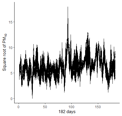
(a) Univariate time series plot

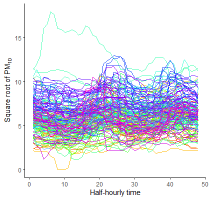
(b) Functional time series plot

Figure 2: Observed time series of (square-root) $\text{PM}_{10}$ levels

In Hörmann et al. (2015) and Shang (2018), observations of half-hourly $\text{PM}_{10}$ levels as in Figure 2(b) are assumed to come from a functional curve. In general, for a functional time series, the original observations are smoothed before further studies such as FPCA and functional bootstrap. Hence, according to Hörmann et al. (2015) and Shang (2018), there are $182$ temporal dependent functional curves each smoothed from $48$ observations. However, as illustrated in Appendix A of this work, the pre-smoothing results rely heavily on the smoothness condition of the functional curve. When the observations are not dense enough, pre-smoothing may cause a loss of information, especially on local patterns. To maintain the original features of time-series observations to the greatest extent, we treat the data as a multivariate or high-dimensional time series. We then perform the proposed AR-sieve bootstrap methods with a factor model on this $48$ by $182$ matrix of time series. This creates a bootstrap confidence interval for the mean levels of (square root) $\text{PM}_{10}$ which are temporal dependent at each half-hourly time point, and to create a bootstrap confidence surface for the lag-$1$ autocovariance matrix of (square root) $\text{PM}_{10}$ levels.

In Figure 3, a $90\%$ nonparametric bootstrap interval using quantiles is created on the mean levels of (square root) $\text{PM}_{10}$, defined as $\theta_{y}\coloneqq\bm{Q}\bm{\mu}_{f}$ with $\bm{\mu}_{f}$ denoting the population mean of temporal dependent factors $\{\bm{f}_{t}\}$. From this plot of sample estimate and confidence interval of $\theta_{y}$, it is clear that local patterns, for example, between $4$^th and $10$^th half-hourly time points, are preserved flawlessly by our proposed AR-sieve bootstrap methods based on high-dimensional time series. Similarly, a sample estimate and a $90\%$ unreversed nonparametric bootstrap interval using quantiles for lag-$1$ autocovariance matrix $\text{Cov}(\bm{y}_{t},\bm{y}_{t+1})$ of temporal dependent (square root) $\text{PM}_{10}$ levels at $48$ half-hourly time points are also computed and presented in Figure 4. This unreversed nonparametric bootstrap interval using quantiles provides interval estimates on autocovariance of (square root) $\text{PM}_{10}$ levels between two consecutive days, where, as shown in Figure 4, the local patterns are again completely preserved by our proposed AR-sieve bootstrap methods.

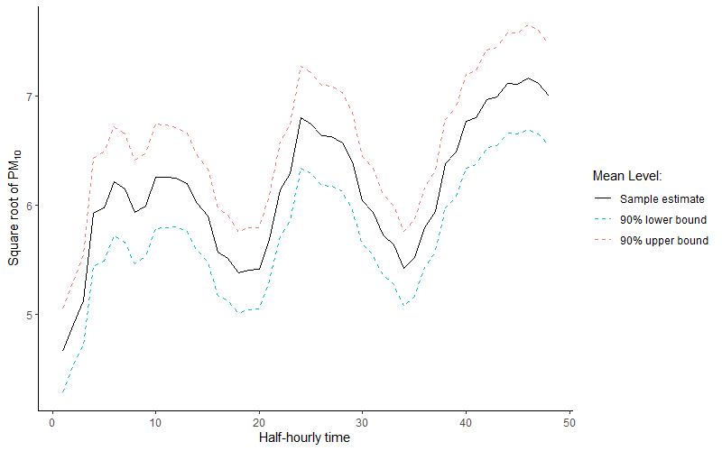
Figure 3: $90\%$ AR-sieve bootstrap confidence interval for the mean of temporal dependent (square root) $\text{PM}_{10}$ levels at $48$ half-hourly time

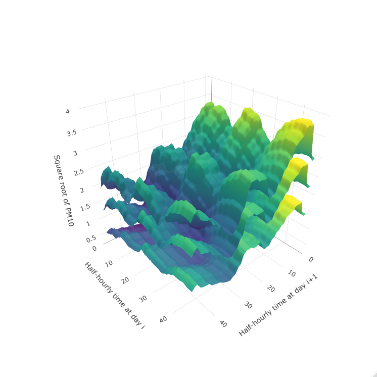
Figure 4: $90\%$ AR-sieve bootstrap confidence surface for lag-$1$ autocovariance of temporal dependent (square root) $\text{PM}_{10}$ levels at $48$ half-hourly time point

7 Conclusions and discussions

We apply dimension-reduction methods, such as factor models, to pursue a new approach - AR-sieve bootstrap on high-dimensional data. Specifically, we suggest using autocovariance to estimate the factor model and perform an AR-sieve bootstrap on the estimated factors to provide ultimate inferences on the original time series. Our proposed AR-sieve bootstrap methods using factor models provide valid statistical inferences on the mean statistic and maintain consistency on bootstrap estimates of spiked eigenvalues of autocovariance matrices. Simulation studies provide numerical evidence on the finite-sample performance of the AR-sieve bootstrap methods on high-dimensional time series following strong factor models. At last, we apply our methods to $\text{PM}_{10}$ data for constructing bootstrap confidence intervals for mean vector and autocovariance matrix, respectively.

Our work is crucial as a building block of bootstrap methods for high-dimensional time series. We propose a low-rank model for AR-sieve bootstrap on high-dimensional stationary time series. There are two ways in which the present paper could be further extended: 1) The asymptotics of the bootstrap validity on the mean statistics can be extended for weaker factor models; 2) While AR-sieve bootstrap is only valid for stationary time series, alternative bootstrap methods can be considered on the factors where the dimension has been reduced.

Supplement to “AR-sieve Bootstrap for High-dimensional Time Series”
Daning Bi, Han Lin Shang, Yanrong Yang, Huanjun Zhu

This supplementary material contains discussions of applying the proposed AR-sieve bootstrap on sparsely-observed functional time series, and technical proofs of results in the original paper “AR-sieve Bootstrap for High-dimensional Time Series”. In Appendix A, we introduce the smoothing problem on sparsely-observed functional time series and then propose to treating it as high-dimensional data when applying the AR-sieve bootstrap. Some simulations are also provided. In Appendix B, proofs of main theorems are presented, while some auxiliary lemmas and their proofs are left in Appendix C.

Appendix A Applications on Sparsely-observed Functional Time Series

The second contribution of this work is that we compare the proposed novel AR-sieve bootstrap for high-dimensional time series with the AR-sieve bootstrap method for functional time series (Paparoditis 2018) in terms of their applications on sparse and unsmoothed functional observations. And we suggest that the sparse and unsmoothed observations need to be treated as high-dimensional time series and the AR-sieve bootstrap proposed in this work needs to be applied. In the literature of functional time series studies, a very fundamental assumption is that the actual observations come from a smoothed functional curve and statistical inferences for functional data usually require the observations to be dense. In a classic functional set-up, dense and discrete points are observed on a sample of $T$ curves. Denoted by $N_{t}$ the number of observations for the curve $t$, the discussions on the density of observations in functional data literature are generally through assumptions made on $N_{t}$. Typically, when $N_{t}$ is much larger than the sample size $T$, the data can be considered dense functional data where each curve can be well smoothed before analysis. However, in the case where $N_{t}$ is small compared with sample size $T$ for all $t$, the discrete observations should be considered as sparse along the population functional curve. The fundamental problem of sparse functional data is that the local patterns of population functional curve are generally not captured by those sparse observations.

To illustrate the potential problems of pre-smoothing sparse observations for functional time series analysis, we consider a toy example. For a square-integrable functional process $\{\mathcal{X}(u),\ u\in\mathcal{I}\}$, let $y_{i,t}$ be the $i$^th observation of $\{\mathcal{X}_{t}(\cdot)\}$, observed at a random time $t$ with the measurement errors defined as $\epsilon_{i,t}$ for $t=1,2,...,T$ and $i=1,2,...,N$. Consider now for a model of functional observations

$$y_{i,t}=\mathcal{X}_{t}(u_{i})+\epsilon_{i,t},\ \ \ u_{i}\in\mathcal{I},$$ (9)

where $\epsilon_{i,t}$ is independent and identically distributed (i.i.d.) with $\mathbb{E}(\epsilon_{i,t})=0$, $\mathbb{V}(\epsilon_{i,t})=\sigma^{2}$ and $\mathcal{I}$ is a functional support. In this model, the observations of $\{\mathcal{X}_{t}(\cdot)\}$ are assumed to be equally spaced, and the number of measurements $N$ assesses the density and design of the actual observations. In the functional data analysis, $\mathcal{X}_{t}(u_{i})$ can be estimated or recovered by some smoothing methods such as a linear smoother as follows,

$$\widehat{\mathcal{X}_{t}}(u_{i})=\sum_{j=1}^{N}w_{i}(u_{j})y_{t,i},$$

where $w_{i}(u_{j})$ is the weight of $j$^th point on the $i$^th point with $\sum_{j=1}^{N}w_{i}(u_{j})=1$ for $t=1,2,...,T$ and $i=1,2,...,N$. The accuracy of the smoothing curve is highly related to the density of observations and measurement errors. If observations along the curve are equally spaced, the change of density can affect the quality of smoothness and its recovering power to the population curve. For a relatively sparse curve, smoothing can fail to work under certain situations; for example, when there are local patterns that observations are too sparse to capture. To visually depict this phenomenon, we provide a toy example by simulations in the following part. We consider a contaminated functional time series model generated from three Fourier bases with different frequencies reflecting local patterns. The details of the simulation setting can be found in Section A.1. The curves in Figure 5 are plotted based on $401$ grid points defined on a functional support $[0,1]$, whereas the actual number of observations $N$ along each curve are chosen as $51$, $21$ and $5$ to address different observation densities.

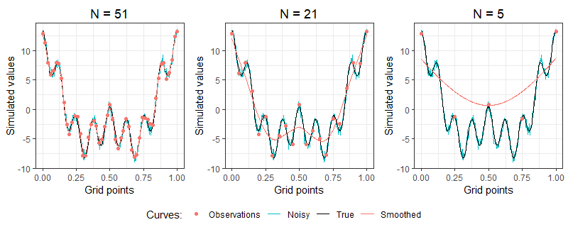
Figure 5: Example of smoothing error of sparse functional time series observations

As shown in Figure 5, when the observations (red points) become sparse (but still equally spaced), the (red) smoothing curve can lead to an obvious misleading result with local patterns not accurately captured by the smoothing curve. The errors associated with pre-smoothing on those sparse observations are generally large. In this situation, the assumption of dense functional data suffers from insufficient observations along each curve. As a result, we cannot adopt the pre-smoothing results based on functional set-up but instead treat the data as multivariate time series with growing dimensions. In other words, when $N$ grows with sample size $T$ but at a relatively slower rate, the real data may adapt to a high-dimensional set-up rather than a functional set-up, which makes statistical inferences and applications rather different. This phenomenon is associated with an area where functional data analysis and high-dimensional data analysis may overlap yet follow different assumptions and produce quite different asymptotic results.

In contrast to functional data analysis, where the increase of observations along a curve can practically improve pre-smoothing and recovering the functional curve, the growing of dimensions is associated with the increase of complexity for high-dimensional data analysis. This key difference makes it vital to choose between functional time series and high-dimensional time series methods. In the following part, we consider the situation where $N$ is growing but not fast enough. The curve smoothed from the sparse observations is inaccurate, especially to local patterns of a functional curve. We apply the proposed AR-sieve bootstrap method for studying the inferences of this type of high-dimensional time series.

A.1 Smoothing on sparse discrete functional time series

To study the impact of smoothing on the sparse functional time series observations, we can compare bootstrap samples’ empirical distributions under various densities of observations. To start, we first assume the data are originated from functional curves, which are temporal dependent. Recall model (9) that

$$y_{t,i}=\mathcal{X}_{t}(u_{i})+\epsilon_{t,i},\ \ \ u_{i}\in\mathcal{I},$$

where $\epsilon_{t,i}$ is i.i.d. with $\mathbb{E}(\epsilon_{t,i})=0$ and $\mathbb{V}(\epsilon_{t,i})=\sigma^{2}$, for $t=1,2,...,T$ and $i=1,2,...,N$. In this model, the number of measurements $N$ reflect the density of the actual observations. To study the impact of density, we assume the observations are equally spaced and generated from a three factors’ model

$$\bm{y}_{t}=\bm{Q}\bm{f}_{t}+\bm{u}_{t},$$

where $u_{t,i}$, the element in $\{\bm{u}_{t}\}$, is independent $\mathcal{N}\ (0,1)$ random noise, $\bm{Q}$ is a $N\times 3$ matrix with each column a Fourier basis and $\cos(2\pi i/N)$, $\cos(4\pi i/N)$, $0.5\cos(16\pi i/N)$ as $i$^th element, respectively. The factors $\{\bm{f}_{t}\}$ follows a VAR(1) model with a coefficient matrix

$$\left[\begin{matrix}0.5&0.1&0.1\\ 0.1&0.5&0.1\\ 0.1&0.1&0.5\\ \end{matrix}\right]$$

and errors independent simulated from $\mathcal{N}\ (0,1)$. The Fourier basis is selected to produce a smoothed population curve, with the third basis reflecting local patterns. Hence, we can generate discrete observations from a functional curve with local patterns. In Section 1, we have presented plots of $\{\bm{y}_{t}\}$ at a particular time $t$ with three different densities of observations to illustrate a smoothing’s potential issue. This section takes it one step further and considers a wider choice of densities so that the actual dimensions of observations along each curve are $N=101,51,21,17,11$ and $5$.

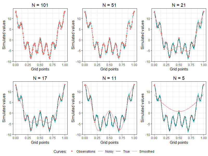
Figure 6: Example of smoothing errors on sparse functional observations

For the same choice of time $t$ as in Section 1, we have generated $6$ plots under various densities in Figure 6 to compare the smoothing results with the population true curve and noisy curve with small measurement errors. The smoothing results are obtained using B-splines with the number of basis functions set to $N$, the actual number of observations in each case, and the roughness penalties selected based on generalised cross-validation (GCV). As depicted in Figure 6, when the actual number of observations $N$ is relatively small, for example, $N<21$, some local patterns of the population curve are generally not captured. In addition, the smoothing curve sometimes also averaged out the actual observations to achieve relatively flat results, for example, when $N=21,17$ and $5$ as in Figure 6. As a result, the observations after smoothing are generally less spread than the original observations, which produces very different bootstrap samples and inferences’ results. To see that, we generate $B=499$ AR-sieve bootstrap samples and computed two summary statistics to compare the bootstrap distribution based on original observations with smoothed observations. We use AR-sieve bootstrap to obtain estimates of a so-called (standardised) mean statistic, computed as $\overline{\overline{y^{\ast}}}=\frac{\sqrt{T}}{\sqrt{N}}\bm{1}^{\top}\bm{\widehat{Q}}\overline{\bm{f}^{\ast}}$ according to Theorem 4.2, and $\delta_{1}^{\ast}$, the estimate of (standardised) largest eigenvalue of symmetrised lag-$1$ sample autocovariance matrix as defined in Proposition 4.4, to compare bootstrap samples from original observations with bootstrap samples from pre-smoothed observations.

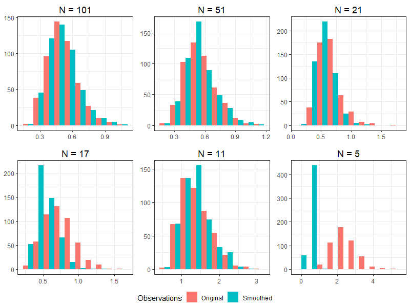
Figure 7: Histograms of $\delta_{1}^{\ast}$, the AR-sieve bootstrap estimates of the largest eigenvalue of symmetrised lag-$1$ sample autocovariance matrix

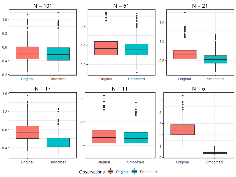
Figure 8: Boxplots of $\delta_{1}^{\ast}$, the AR-sieve bootstrap estimates of the largest eigenvalue of symmetrised lag-$1$ sample autocovariance matrix

Figures 7 and 8 compare the histograms and boxplots of $\delta_{1}^{\ast}$, the AR-sieve bootstrap estimates of largest eigenvalue of symmetrised lag-$1$ autocovariance matrix, while Figures 9 and 10 compare the histograms and boxplots of $\overline{\overline{y^{\ast}}}$, the AR-sieve bootstrap estimates of the (standardised) mean statistic. As seen in Figure 6, when $N=21,17$ and $5$, the pre-smoothed observations are averaged out compared with the original observations. As a result, the bootstrap estimates of the two statistics perform differently before and after smoothing, when $N=21,17$ and $5$. Figures 7 and 9 use boxplots to present the difference of empirical distributions of $\overline{\overline{y^{\ast}}}$ and $\delta_{1}^{\ast}$ for $N=21,17$ and $5$, whereas Figures 8 and 10 illustrate the impact of smoothing by comparing the histograms of $\overline{\overline{y^{\ast}}}$ and $\delta_{1}^{\ast}$.

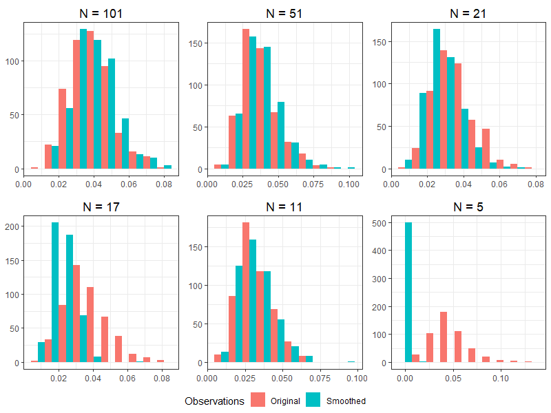
Figure 9: Histograms of $\overline{\overline{y^{\ast}}}$, the AR-sieve bootstrap estimates of the mean statistic

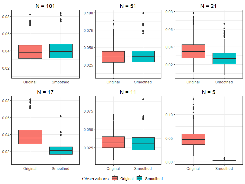
Figure 10: Boxplots of $\overline{\overline{y^{\ast}}}$, the AR-sieve bootstrap estimates of the mean statistic

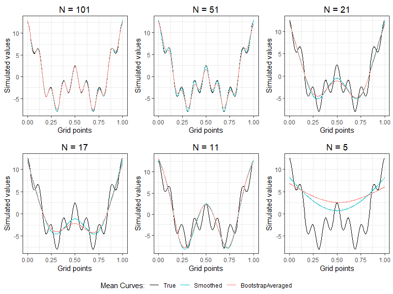
Figure 11: Example of errors of the AR-sieve bootstrap mean curve for sparse functional observations

The last example we presented in Figure 11 illustrates results of AR-sieve bootstrap estimates (bootstrap average) of the functional mean curve when we pre-smooth the observations under various densities of data. As shown in Figure 11, when the actual observations are relatively dense, for example, $N\geq 51$, AR-sieve bootstrap estimates of the mean functional curve are close to the pre-smoothed curve and the population curve. However, when the observations are sparse, for example, $N\leq 21$, AR-sieve bootstrap estimates of the mean functional curve do not correctly capture the local patterns of the population curve, which is due to the unacceptable smoothing results. This result is also typical evidence of the impact of pre-smoothing on AR-sieve bootstrap for functional time series. Hence, when the actual functional time series observations are sparse, pre-smoothing may significantly impact statistical inferences, including bootstrap. In fact, for many real-world time series data, the rule on considering a data set as dense functional time series is generally not clear and often varies across researchers and problems. Practically speaking, the impact of observations’ density is only about whether to pre-smooth the functional time series before performing bootstrap or other statistical analysis.

Nonetheless, the theoretical assumptions behind functional time series and high-dimensional time series vary, leading to very different theoretical results on statistical inferences, including AR-sieve bootstrap. On the other hand, this difference in data structure assumptions demonstrates the importance of developing statistical methods on sparse functional time series observations. It verifies our contributions on the building blocks of AR-sieve bootstrap for high-dimensional time series.

Appendix B Technical proof of theorems

Proof of Theorem 4.2.

Let $\bm{f}^{b}_{t}=\sum_{l=1}^{p}\bm{\widetilde{A}}_{l,p}\bm{f}^{b}_{t-l}+\bm{e}^{b}_{t,p}$, where $\{\bm{\widetilde{A}}_{l,p},\ l=1,2,...,p\}$ are the estimators of AR coefficient matrices based on true factors $\{\bm{f}_{t}\}$, and $\{\bm{e}^{b}_{t,p},t=p+1,p+2,...,T\}$ are generated by i.i.d. resampling from the centered residuals $(\bm{\widetilde{e}}_{t,p}-\overline{\bm{\widetilde{e}}}_{T,p})$ with $\bm{\widetilde{e}}_{t,p}=\bm{f}_{t}-\sum_{l=1}^{p}\bm{\widetilde{A}}\bm{f}_{t-l}$ and $\overline{\bm{\widetilde{e}}}_{T,p}=\frac{1}{T-p}\sum_{t=p+1}^{T}\bm{\widetilde{e}}_{t,p}$. Therefore, $\{\bm{f}^{b}_{t}\}$ are bootstrap pseudo-variables generated based on the true factors $\{\bm{f}_{t}\}$ rather than $\{\bm{\widehat{f}}_{t}\}$. Recall that $\{\bm{f}^{\ast}_{t}\}$ are bootstrapped based on the centered residuals $(\bm{\widehat{e}}_{t,p}-\overline{\bm{\widehat{e}}}_{T,p})$ with $\bm{\widehat{e}}_{t,p}=\bm{\widehat{f}}_{t}-\sum_{l=1}^{p}\bm{\widehat{A}}_{l,p}\bm{\widehat{f}}_{t-l}$ and $\overline{\bm{\widehat{e}}}_{T,p}=\frac{1}{T-p}\sum_{t=p+1}^{T}\bm{\widehat{e}}_{t,p}$, and we define $\mathbb{E}^{\ast}$ and $\text{Cov}^{\ast}$ as the expectation and covariance with respect to the measure assigning probability $1/(T-p)$ to each observation, respectively. Therefore, $\mathbb{E}^{\ast}\overline{\bm{f}^{\ast}_{T}}=\overline{\bm{\widehat{f}}_{T}}$ by definition and we can write

$$\sqrt{T}\bm{c}^{\top}\bm{\widehat{Q}}\left(\overline{\bm{f}^{\ast}_{T}}-\mathbb{E}^{\ast}\overline{\bm{f}^{\ast}_{T}}\right) \eqqcolon\mathcal{M}_{1}+\mathcal{M}_{2}+\mathcal{M}_{3}$$

$$=\sqrt{T}\bm{c}^{\top}\bm{Q}\left(\overline{\bm{f}^{b}_{T}}-\mathbb{E}^{\ast}\overline{\bm{f}^{b}_{T}}\right)+\sqrt{T}\bm{c}^{\top}\left(\bm{\widehat{Q}}-\bm{Q}\right)\left(\overline{\bm{f}^{\ast}_{T}}-\mathbb{E}^{\ast}\overline{\bm{f}^{\ast}_{T}}\right)$$

$$+\sqrt{T}\bm{c}^{\top}\bm{Q}\left[\left(\overline{\bm{f}^{\ast}_{T}}-\mathbb{E}^{\ast}\overline{\bm{f}^{\ast}_{T}}\right)-\left(\overline{\bm{f}^{b}_{T}}-\mathbb{E}^{\ast}\overline{\bm{f}^{b}_{T}}\right)\right],$$

with obvious definitions of $\mathcal{M}_{1},\mathcal{M}_{2}$ and $\mathcal{M}_{3}$.

For the term $\mathcal{M}_{1}$, under Assumptions 3.1 (iii), 4.1 and the additional assumption in Theorem 4.2 that $\lim_{T\to\infty}\mathbb{V}(\sqrt{T}\overline{\bm{f}_{T}})=\sum_{k\in\mathbf{Z}}\bm{\Gamma}_{\bm{f}}(k)<\infty$, using Theorem 2.1 in Politis et al. (1997), we have the following CLT for $\sqrt{T}\ \overline{\bm{f}_{T}}$

$$\sqrt{T}\left(\overline{\bm{f}_{T}}-\mathbb{E}\overline{\bm{f}_{T}}\right)\overset{d}{\to}\mathcal{N}\ \left(0,\ \sum_{k\in\mathbf{Z}}\bm{\Gamma}_{\bm{f}}(k)\right).$$

Moreover, under the additional assumptions in Theorem 4.2, $\bm{c}^{\top}\bm{Q}$ is an $r$-dimensional vector such that $\|\bm{c}^{\top}\bm{Q}\|_{\ell_{1}}<\infty$ for a fixed $r$, Therefore, under Assumptions 3.1 (ii) and 4.1, we can use Cramer-Wold Theorem (Cramér & Wold 1936) to conclude for the scalar $\sqrt{T}\bm{c}^{\top}\bm{Q}\overline{\bm{f}_{T}}$ that

$$\sqrt{T}\bm{c}^{\top}\bm{Q}\left(\overline{\bm{f}_{T}}-\mathbb{E}\overline{\bm{f}_{T}}\right)\overset{d}{\to}\mathcal{N}\ \left(0,\ \bm{c}^{\top}\bm{Q}\left(\sum_{k\in\mathbf{Z}}\bm{\Gamma}_{\bm{f}}(k)\right)\bm{Q}^{\top}\bm{c}\right),$$

when $T,N\to\infty$.

Besides, under the strong mixing condition on true factors $\{\bm{f}_{t}\}$, the empirical moments of $\{\bm{e}_{t}\}$ converge to its population counterpart. Therefore, under all the assumptions of 4.2, we fulfil all the conditions of Theorem 4.1 in Meyer & Kreiss (2015). Consequently, we can use Theorem 4.1 in Meyer & Kreiss (2015) to conclude that the general VAR-sieve bootstrap is valid for $\sqrt{T}\bm{c}^{\top}\bm{Q}\overline{\bm{f}_{T}}$ since $\sqrt{T}\bm{c}^{\top}\bm{Q}\overline{\bm{f}_{T}}$ shares the same CLT with its counterpart generated from the companion process as discussed in Meyer & Kreiss (2015). Hence

$$d_{K}\left(\mathcal{L}\left(\left.\sqrt{T}\bm{c}^{\top}\bm{\widehat{Q}}\left(\overline{\bm{f}^{\ast}_{T}}-\mathbb{E}^{\ast}\overline{\bm{f}^{\ast}_{T}}\right)\right|\bm{y}_{1},\bm{y}_{2},...,\bm{y}_{T}\right),\mathcal{L}\left(\sqrt{T}\bm{c}^{\top}\bm{Q}\left(\overline{\bm{f}_{T}}-\mathbb{E}\overline{\bm{f}_{T}}\right)\right)\right)=o_{P}\left(1\right)$$

as $T,N\to\infty$.

Therefore, to see the assertion in Theorem 4.2, we need to show that when $T,N\to\infty$, both $\mathcal{M}_{2}$ and $\mathcal{M}_{3}$ tend to $0$ in probability, then apply Slutsky’s theorem.

To show $\mathcal{M}_{2}\to 0$ in probability for $T,N\to\infty$, we first of all notice that

$$\sqrt{T}\bm{c}^{\top}\left(\bm{\widehat{Q}}-\bm{Q}\right)\left(\overline{\bm{f}^{\ast}_{T}}-\mathbb{E}^{\ast}\overline{\bm{f}^{\ast}_{T}}\right)=\frac{1}{\sqrt{T}}\bm{c}^{\top}\left(\bm{\widehat{Q}}-\bm{Q}\right)\sum_{t=1}^{T}\left(\bm{f}^{\ast}_{t}-\overline{\bm{\widehat{f}}_{T}}\right).$$

Therefore, we can show that

$$\mathbb{E}\left[\sqrt{T}\bm{c}^{\top}\left(\bm{\widehat{Q}}-\bm{Q}\right)\left(\overline{\bm{f}^{\ast}_{T}}-\mathbb{E}\overline{\bm{f}^{\ast}_{T}}\right)\right]^{2}$$

$$= \mathbb{E}\left[\frac{1}{T}\bm{c}^{\top}\left(\bm{\widehat{Q}}-\bm{Q}\right)\sum_{t=1}^{T}\left(\bm{f}^{\ast}_{t}-\overline{\bm{\widehat{f}}_{T}}\right)\right]\left[\sum_{s=1}^{T}\left(\bm{f}^{\ast}_{s}-\overline{\bm{\widehat{f}}_{T}}\right)^{\top}\left(\bm{\widehat{Q}}-\bm{Q}\right)^{\top}\bm{c}\right]$$

$$= \left[\frac{1}{T}\bm{c}^{\top}\left(\bm{\widehat{Q}}-\bm{Q}\right)\sum_{t=1}^{T}\sum_{s=1}^{T}\mathbb{E}\left(\bm{f}^{\ast}_{t}-\overline{\bm{\widehat{f}}_{T}}\right)\left(\bm{f}^{\ast}_{s}-\overline{\bm{\widehat{f}}_{T}}\right)^{\top}\left(\bm{\widehat{Q}}-\bm{Q}\right)^{\top}\bm{c}\right]$$

$$\leq \frac{1}{T}\left\|\bm{c}^{\top}\left(\bm{\widehat{Q}}-\bm{Q}\right)\right\|^{2}\left\|\sum_{t=1}^{T}\sum_{s=1}^{T}\mathbb{E}\left(\bm{f}^{\ast}_{t}-\overline{\bm{\widehat{f}}_{T}}\right)\left(\bm{f}^{\ast}_{s}-\overline{\bm{\widehat{f}}_{T}}\right)^{\top}\right\|_{F}$$

$$= O_{P}\left(\frac{1}{T^{2}}\left\|\sum_{t=1}^{T}\sum_{s=1}^{T}\mathbb{E}\left(\bm{f}^{\ast}_{t}-\overline{\bm{\widehat{f}}_{T}}\right)\left(\bm{f}^{\ast}_{s}-\overline{\bm{\widehat{f}}_{T}}\right)^{\top}\right\|_{F}\right),$$

Define ${\Sigma}_{e,p}^{\ast}\coloneqq\mathbb{E}^{\ast}\left(\bm{e}^{\ast}_{t}\bm{e}_{t}^{\ast\top}\right)$, then

$$\sum_{t=1}^{T}\sum_{s=1}^{T}\mathbb{E}^{\ast}\left(\bm{f}^{\ast}_{t}-\overline{\bm{\widehat{f}}_{T}}\right)\left(\bm{f}^{\ast}_{s}-\overline{\bm{\widehat{f}}_{T}}\right)^{\top}= \sum_{t=1}^{T}\sum_{s=1}^{T}\mathbb{E}^{\ast}\left(\left(\sum_{l_{1}=0}^{\infty}\bm{\widehat{\Psi}}_{l_{1},p}\bm{e}^{\ast}_{t-l_{1}}\right)\left(\sum_{l_{2}=0}^{\infty}\bm{\widehat{\Psi}}_{l_{2},p}\bm{e}^{\ast}_{s-l_{2}}\right)^{\top}\right)$$

$$= \sum_{t=1}^{T}\sum_{s=1}^{T}\mathbb{E}^{\ast}\sum_{l_{1}=0}^{\infty}\sum_{l_{2}=0}^{\infty}\left(\bm{\widehat{\Psi}}_{l_{1},p}\bm{e}^{\ast}_{t-l_{1}}\bm{e}_{s-l_{2}}^{\ast\top}\bm{\widehat{\Psi}}_{l_{2},p}^{\top}\right)$$

$$= \sum_{t=1}^{T}\sum_{s=1}^{T}\sum_{l=0}^{\infty}\bm{\widehat{\Psi}}_{l,p}\mathbb{E}^{\ast}\left(\bm{e}^{\ast}_{t-l}\bm{e}_{t-l}^{\ast\top}\right)\bm{\widehat{\Psi}}_{s-t+l,p}^{\top}$$

where $\bm{e}^{\ast}_{t-l_{1}}$ and $\bm{e}^{\ast}_{t-l_{2}}$ are i.i.d. bootstrapped therefore $\mathbb{E}^{\ast}\left(\bm{e}^{\ast}_{t-l_{1}}\bm{e}_{t-l_{2}}^{\ast\top}\right)=\mathbf{0}$ for $l_{1}\neq l_{2}$.

Hence we can show that

$$\frac{1}{T^{2}}\left\|\sum_{t=1}^{T}\sum_{s=1}^{T}\mathbb{E}^{\ast}\left(\bm{f}^{\ast}_{t}-\overline{\bm{\widehat{f}}_{T}}\right)\left(\bm{f}^{\ast}_{s}-\overline{\bm{\widehat{f}}_{T}}\right)^{\top}\right\|_{F}\leq \frac{1}{T^{2}}\left\|{\Sigma}_{e,p}^{\ast}\right\|_{F}\sum_{l=0}^{\infty}\left\|\bm{\widehat{\Psi}}_{l,p}\right\|_{F}\sum_{t=1}^{T}\sum_{s=1}^{T}\left\|\bm{\widehat{\Psi}}_{s-t+l,p}\right\|_{F}$$

$$= O_{P}\left(\frac{1}{T}\right),$$

where we note that Lemmas C.5 and C.7 imply the summability of $\left\|\bm{\widehat{\Psi}}_{l,p}\right\|_{F}$, hence $\sum_{s=1}^{T}\left\|\bm{\widehat{\Psi}}_{s-t+l,p}\right\|_{F}$ is bounded for $T\to\infty$. Therefore, $\frac{1}{T}\sum_{l=0}^{\infty}\left\|\bm{\widehat{\Psi}}_{l,p}\right\|_{F}\sum_{t=1}^{T}\sum_{s=1}^{T}\left\|\bm{\widehat{\Psi}}_{s-t+l,p}\right\|_{F}$ is bounded for $T\to\infty$, and we can conclude that $\mathbb{E}^{\ast}\left[\sqrt{T}\bm{c}^{\top}\left(\bm{\widehat{Q}}-\bm{Q}\right)\left(\overline{\bm{f}^{\ast}_{T}}-\mathbb{E}^{\ast}\overline{\bm{f}^{\ast}_{T}}\right)\right]^{2}\to 0$ in probability, which suffices for $\mathcal{M}_{2}\to 0$ in probability conditional on the sample.

For $\mathcal{M}_{3}$, we first write

$$\mathbb{E}^{\ast}\left[\sqrt{T}\bm{c}^{\top}\bm{Q}\left\{\left(\overline{\bm{f}^{\ast}_{T}}-\mathbb{E}^{\ast}\overline{\bm{f}^{\ast}_{T}}\right)-\left(\overline{\bm{f}^{b}_{T}}-\mathbb{E}^{\ast}\overline{\bm{f}^{b}_{T}}\right)\right\}\right]^{2}$$

$$= \mathbb{E}^{\ast}\left\|\sqrt{T}\bm{c}^{\top}\bm{Q}\left\{\left(\overline{\bm{f}^{\ast}_{T}}-\overline{\bm{\widehat{f}}_{T}}\right)-\left(\overline{\bm{f}^{b}_{T}}-\overline{\bm{\widetilde{f}}_{T}}\right)\right\}\right\|^{2}$$

$$\leq \|\bm{c}^{\top}\bm{Q}\|^{2}\frac{1}{T}\sum_{t=1}^{T}\sum_{s=1}^{T}\mathbb{E}^{\ast}\left\|\left\{\left(\bm{f}^{\ast}_{t}-\overline{\bm{\widehat{f}}_{T}}\right)-\left(\bm{f}^{b}_{t}-\overline{\bm{\widetilde{f}}_{T}}\right)\right\}\left\{\left(\bm{f}^{\ast}_{s}-\overline{\bm{\widehat{f}}_{T}}\right)-\left(\bm{f}^{b}_{s}-\overline{\bm{\widetilde{f}}_{T}}\right)\right\}^{\top}\right\|_{F}$$

$$= O_{P}\left(\frac{1}{T}\sum_{t=1}^{T}\sum_{s=1}^{T}\mathbb{E}^{\ast}\left\|\left\{\left(\bm{f}^{\ast}_{t}-\overline{\bm{\widehat{f}}_{T}}\right)-\left(\bm{f}^{b}_{t}-\overline{\bm{\widetilde{f}}_{T}}\right)\right\}\left\{\left(\bm{f}^{\ast}_{s}-\overline{\bm{\widehat{f}}_{T}}\right)-\left(\bm{f}^{b}_{s}-\overline{\bm{\widetilde{f}}_{T}}\right)\right\}^{\top}\right\|_{F}\right),$$

where the last line follows from the fact that $\|\bm{c}^{\top}\bm{Q}\|^{2}$ is bounded when $N\to\infty$. To proceed, first note that

$$\frac{1}{T}\sum_{t=1}^{T}\sum_{s=1}^{T}\mathbb{E}^{\ast}\left\{\left(\bm{f}^{\ast}_{t}-\overline{\bm{\widehat{f}}_{T}}\right)-\left(\bm{f}^{b}_{t}-\overline{\bm{\widetilde{f}}_{T}}\right)\right\}\left\{\left(\bm{f}^{\ast}_{s}-\overline{\bm{\widehat{f}}_{T}}\right)-\left(\bm{f}^{b}_{s}-\overline{\bm{\widetilde{f}}_{T}}\right)\right\}^{\top}$$

$$= \frac{1}{T}\sum_{t=1}^{T}\sum_{s=1}^{T}\mathbb{E}^{\ast}\left\{\sum_{l_{1}=0}^{\infty}\bm{\widehat{\Psi}}_{l_{1},p}\bm{e}^{\ast}_{t-l_{1},p}-\bm{\widetilde{\Psi}}_{l_{1},p}\bm{e}^{b}_{t-l_{1},p}\right\}\left\{\sum_{l_{2}=0}^{\infty}\bm{\widehat{\Psi}}_{l_{2},p}\bm{e}^{\ast}_{s-l_{2},p}-\bm{\widetilde{\Psi}}_{l_{2},p}\bm{e}^{b}_{s-l_{2},p}\right\}^{\top}$$

$$= \frac{1}{T}\sum_{t=1}^{T}\sum_{s=1}^{T}\mathbb{E}^{\ast}\left\{\sum_{l_{1}=0}^{\infty}\bm{\widehat{\Psi}}_{l_{1},p}\bm{e}^{\ast}_{t-l_{1},p}\right\}\left\{\sum_{l_{2}=0}^{\infty}\bm{\widehat{\Psi}}_{l_{2},p}\bm{e}^{\ast}_{s-l_{2},p}-\bm{\widetilde{\Psi}}_{l_{2},p}\bm{e}^{b}_{s-l_{2},p}\right\}^{\top}$$

$$+ \frac{1}{T}\sum_{t=1}^{T}\sum_{s=1}^{T}\mathbb{E}^{\ast}\left\{\sum_{l_{1}=0}^{\infty}\bm{\widetilde{\Psi}}_{l_{1},p}\bm{e}^{b}_{t-l_{1},p}\right\}\left\{\sum_{l_{2}=0}^{\infty}\bm{\widetilde{\Psi}}_{l_{2},p}\bm{e}^{b}_{s-l_{2},p}-\bm{\widehat{\Psi}}_{l_{2},p}\bm{e}^{\ast}_{s-l_{2},p}\right\}^{\top}$$

$$\eqqcolon \frac{1}{T}\sum_{t=1}^{T}\sum_{s=1}^{T}\left(\mathcal{H}_{1}+\mathcal{H}_{2}\right),$$

with an obvious notation for $\mathcal{H}_{1}$ and $\mathcal{H}_{2}$. Then, we only consider $\mathcal{H}_{1}$ as $\mathcal{H}_{2}$ can be dealt with similarly.

For $\mathcal{H}_{1}$, we can further decompose it as

$$\mathcal{H}_{1}= \sum_{s=1}^{T}\mathbb{E}^{\ast}\left\{\sum_{l_{1}=0}^{\infty}\bm{\widehat{\Psi}}_{l_{1},p}\bm{e}^{\ast}_{t-l_{1},p}\right\}\left\{\sum_{l_{2}=0}^{\infty}\bm{\widehat{\Psi}}_{l_{2},p}\bm{e}^{\ast}_{s-l_{2},p}-\bm{\widetilde{\Psi}}_{l_{2},p}\bm{e}^{\ast}_{s-l_{2},p}\right\}^{\top}$$

$$+ \sum_{s=1}^{T}\mathbb{E}^{\ast}\left\{\sum_{l_{1}=0}^{\infty}\bm{\widehat{\Psi}}_{l_{1},p}\bm{e}^{\ast}_{t-l_{1},p}\right\}\left\{\sum_{l_{2}=0}^{\infty}\bm{\widetilde{\Psi}}_{l_{2},p}\bm{e}^{\ast}_{s-l_{2},p}-\bm{\widetilde{\Psi}}_{l_{2},p}\bm{e}^{b}_{s-l_{2},p}\right\}^{\top}$$

$$= \sum_{s=1}^{T}\sum_{l=0}^{\infty}\bm{\widehat{\Psi}}_{l,p}\mathbb{E}^{\ast}\left\{\bm{e}^{\ast}_{t-l,p}\bm{e}_{t-l,p}^{\ast\top}\right\}\left\{\bm{\widehat{\Psi}}_{l+s-t,p}-\bm{\widetilde{\Psi}}_{l+s-t,p}\right\}^{\top}$$

$$+ \sum_{s=1}^{T}\sum_{l=0}^{\infty}\bm{\widehat{\Psi}}_{l,p}\mathbb{E}^{\ast}\left\{\bm{e}^{\ast}_{t-l,p}(\bm{e}^{\ast}_{t-l,p}-\bm{e}^{b}_{t-l,p})^{\top}\right\}\bm{\widetilde{\Psi}}_{l+s-t,p}^{\top}$$

$$\eqqcolon \mathcal{H}_{11}+\mathcal{H}_{12}.$$

where the second last line follows from the bootstrap independence for $l_{1}\neq l_{2}$. Hence we can conclude for $\mathcal{H}_{11}$ that

$$\frac{1}{T}\sum_{t=1}^{T}\sum_{s=1}^{T}\left\|\mathcal{H}_{11}\right\|_{F}= \frac{1}{T}\sum_{t=1}^{T}\sum_{s=1}^{T}\left\|\sum_{l=0}^{\infty}\bm{\widehat{\Psi}}_{l,p}{\Sigma}_{e,p}^{\ast}\left\{\bm{\widehat{\Psi}}_{l+s-t,p}-\bm{\widetilde{\Psi}}_{l+s-t,p}\right\}^{\top}\right\|_{F}$$

$$\leq \left\|{\Sigma}_{e,p}^{\ast}\right\|_{F}\frac{1}{T}\sum_{l=0}^{\infty}\left\|\bm{\widehat{\Psi}}_{l,p}\right\|_{F}\sum_{t=1}^{T}\sum_{s=1}^{T}\left\|\bm{\widehat{\Psi}}_{l+s-t,p}-\bm{\widetilde{\Psi}}_{l+s-t,p}\right\|_{F}$$

$$= O_{P}\left(p^{\frac{3}{2}}\left\|\bm{\widehat{A}}_{p}-\bm{\widetilde{A}}_{p}\right\|_{F}\right)$$

$$= o_{P}\left(1\right),$$

where the second last line follows from the results in Lemmas C.5 and C.7, and the last line follows the result in Lemma C.7.

For $\mathcal{H}_{12}$ we can show that

$$\frac{1}{T}\sum_{t=1}^{T}\sum_{s=1}^{T}\left\|\mathcal{H}_{12}\right\|_{F}\leq \sqrt{\mathbb{E}^{\ast}\left\|\bm{e}^{\ast}_{t,p}\right\|^{2}}\sqrt{\mathbb{E}^{\ast}\left\|\bm{e}^{\ast}_{t,p}-\bm{e}^{b}_{t,p}\right\|^{2}}\frac{1}{T}\sum_{l=0}^{\infty}\left\|\bm{\widehat{\Psi}}_{l,p}\right\|_{F}\sum_{t=1}^{T}\sum_{s=1}^{T}\left\|\bm{\widehat{\Psi}}_{l+s-t,p}\right\|_{F}$$

$$= O_{P}\left(\sqrt{\mathbb{E}^{\ast}\left\|\bm{e}^{\ast}_{t,p}-\bm{e}^{b}_{t,p}\right\|^{2}}\right),$$

where the last line follows from the same arguments on summability properties in Lemmas C.5. Hence it remains to show $\mathbb{E}^{\ast}\left\|\bm{e}^{\ast}_{t,p}-\bm{e}^{b}_{t,p}\right\|^{2}\to 0$ in probability. Recall that $\mathbb{E}^{\ast}$ defines expectation with respect to the measure assigning probability $1/(T-p)$ to each observation, this follows as

$$\mathbb{E}^{\ast}\left\|\bm{e}^{\ast}_{t,p}-\bm{e}^{b}_{t,p}\right\|^{2}= \mathbb{E}^{\ast}\left\{\left(\bm{e}^{\ast}_{t,p}-\bm{e}^{b}_{t,p}\right)\left(\bm{e}^{\ast}_{t,p}-\bm{e}^{b}_{t,p}\right)^{\top}\right\}$$

$$= \frac{1}{T-p}\sum_{t=p+1}^{T}\left\{(\bm{\widehat{e}}_{t,p}-\overline{\bm{\widehat{e}}}_{T,p})-(\bm{\widetilde{e}}_{t,p}-\overline{\bm{\widetilde{e}}}_{T,p})\right\}\left\{(\bm{\widehat{e}}_{t,p}-\overline{\bm{\widehat{e}}}_{T,p})-(\bm{\widetilde{e}}_{t,p}-\overline{\bm{\widetilde{e}}}_{T,p})\right\}^{\top}$$

$$= \frac{1}{T-p}\sum_{t=p+1}^{T}\left\{(\bm{\widehat{e}}_{t,p}-\bm{\widetilde{e}}_{t,p})-(\overline{\bm{\widehat{e}}}_{T,p}-\overline{\bm{\widetilde{e}}}_{T,p})\right\}\left\{(\bm{\widehat{e}}_{t,p}-\bm{\widetilde{e}}_{t,p})-(\overline{\bm{\widehat{e}}}_{T,p}-\overline{\bm{\widetilde{e}}}_{T,p})\right\}^{\top}$$

$$\leq \frac{2}{T-p}\sum_{t=p+1}^{T}\left\|\bm{\widehat{e}}_{t,p}-\bm{\widetilde{e}}_{t,p}\right\|^{2}+2\left\{\left\|\overline{\bm{\widetilde{e}}}_{T,p}\right\|^{2}+\left\|\overline{\bm{\widehat{e}}}_{T,p}\right\|^{2}-2\left\|\overline{\bm{\widetilde{e}}}_{T,p}\right\|\left\|\overline{\bm{\widehat{e}}}_{T,p}\right\|\right\}$$

$$\leq \frac{2}{T-p}\sum_{t=p+1}^{T}\left\|\bm{\widehat{e}}_{t,p}-\bm{\widetilde{e}}_{t,p}\right\|^{2}+4\left\{\left\|\overline{\bm{\widetilde{e}}}_{T,p}\right\|^{2}+\left\|\overline{\bm{\widehat{e}}}_{T,p}\right\|^{2}\right\}.$$

Recall that when $\{\bm{f}_{t}\}$ and $\{\bm{\widehat{f}}_{t}\}$ have non-zero means, $\bm{\widetilde{e}}_{t,p}=\left(\bm{f}_{t}-\overline{\bm{f}_{T}}\right)-\sum_{l=1}^{p}\bm{\widetilde{A}}_{l,p}\left(\bm{f}_{t-l}-\overline{\bm{f}}_{T}\right)$ and $\bm{\widehat{e}}_{t,p}=\left(\bm{\widehat{f}}_{t}-\overline{\bm{\widehat{f}}_{T}}\right)-\sum_{l=1}^{p}\bm{\widehat{A}}_{l,p}\left(\bm{\widehat{f}}_{t-l}-\overline{\bm{\widehat{f}}}_{T}\right)$. Without altering the idea of proof, to simplify the notations used, we use $\{\bm{f}_{t}\}$ and $\{\bm{\widehat{f}}_{t}\}$ to denote the demeaned factors $\left(\bm{f}_{t}-\overline{\bm{f}_{T}}\right)$ and their sample counterparts $\left(\bm{\widehat{f}}_{t}-\overline{\bm{\widehat{f}}_{T}}\right)$, respectively. Therefore, with the same arguments in the proof of Lemma C.8, we have

$$\frac{2}{T-p}\sum_{t=p+1}^{T}\left\|\bm{\widehat{e}}_{t,p}-\bm{\widetilde{e}}_{t,p}\right\|^{2}= \frac{2}{T-p}\sum_{t=p+1}^{T}\left\|(\bm{\widehat{f}}_{t}-\bm{f}_{t})+\sum_{l=1}^{p}(\bm{\widetilde{A}}_{l,p}\bm{f}_{t-l}-\bm{\widehat{A}}_{l,p}\bm{\widehat{f}}_{t-l})\right\|^{2}$$

$$\leq \frac{4}{T-p}\sum_{t=p+1}^{T}\left\|\bm{\widehat{f}}_{t}-\bm{f}_{t}\right\|^{2}+\frac{4}{T-p}\sum_{t=p+1}^{T}\left\|\sum_{l=1}^{p}\bm{\widetilde{A}}_{l,p}\bm{f}_{t-l}-\bm{\widehat{A}}_{l,p}\bm{\widehat{f}}_{t-l}\right\|^{2}$$

$$\leq \frac{4}{T-p}\sum_{t=p+1}^{T}\left\|\bm{\widehat{f}}_{t}-\bm{f}_{t}\right\|^{2}+8\sum_{l=1}^{p}\left\|\bm{\widehat{A}}_{l,p}\right\|_{F}^{2}\frac{1}{T-p}\sum_{t=p+1}^{T}\left\|\bm{\widehat{f}}_{t-l}-\bm{f}_{t-l}\right\|^{2}$$

$$+ 8\left\|\sum_{l=1}^{p}\left(\bm{\widehat{A}}_{l,p}-\bm{\widetilde{A}}_{l,p}\right)\frac{1}{T-p}\sum_{t=p+1}^{T}\bm{f}_{t-l}\right\|_{F}^{2}$$

$$= O_{P}\left(\sup_{p+1\leq t\leq T}\left\|\bm{\widehat{f}}_{t}-\bm{f}_{t}\right\|^{2}\right)+O_{P}\left(\left\|\sum_{l=1}^{p}\left(\bm{\widehat{A}}_{p}-\bm{\widetilde{A}}_{p}\right)\right\|_{F}^{2}\right)$$

$$= O_{P}\left(\left(\frac{1}{\sqrt{T}}+\frac{1}{\sqrt{N}}\right)^{2}\right)+O_{P}\left(p^{8}\left(\frac{1}{\sqrt{T}}+\frac{1}{\sqrt{N}}\right)^{2}\right)$$

$$= o_{P}(1),$$ (10)

where the third last line follows from the fact that $\left\|\bm{\widehat{A}}_{l,p}\right\|_{F}^{2}$ is summable, which is implied by Assumption 4.2 and Lemma C.3. The second last line is then a direct result of Lemmas C.3 and C.4, and Assumption 4.3 implies the last line.

Furthermore, $\overline{\bm{\widehat{e}}}_{T,p}=\frac{1}{T-p}\sum_{t=p+1}^{T}\bm{\widehat{e}}_{t,p}=\frac{1}{T-p}\sum_{t=p+1}^{T}\left(\bm{\widehat{f}}_{t}-\sum_{l=1}^{p}\bm{\widehat{A}}_{l,p}\bm{\widehat{f}}_{t-l}\right)$ and we can show that

$$\left\|\overline{\bm{\widehat{e}}}_{T,p}\right\|^{2}\leq 2\left\|\frac{1}{T-p}\sum_{t=p+1}^{T}\bm{\widehat{f}}_{t}\right\|^{2}+2\left\|\sum_{l=1}^{p}\bm{\widehat{A}}_{l,p}\frac{1}{T-p}\sum_{t=p+1}^{T}\bm{\widehat{f}}_{t-l}\right\|^{2}=o_{P}(1).$$ (11)

This is because, firstly

$$\left\|\frac{1}{T-p}\sum_{t=p+1}^{T}\bm{\widehat{f}}_{t}\right\|^{2}\leq 2\left\|\frac{1}{T-p}\sum_{t=p+1}^{T}\bm{f}_{t}\right\|^{2}+2\left\|\frac{1}{T-p}\sum_{t=p+1}^{T}\left(\bm{\widehat{f}}_{t}-\bm{f}_{t}\right)\right\|^{2}$$

$$= O_{P}\left(\frac{1}{T-p}\right)+O_{P}\left(\frac{1}{T-p}\sum_{t=p+1}^{T}\left\|\bm{\widehat{f}}_{t}-\bm{f}_{t}\right\|^{2}\right)$$

$$= O_{P}\left(\frac{1}{T-p}\right)+O_{P}\left(\left(\frac{1}{\sqrt{T}}+\frac{1}{\sqrt{N}}\right)^{2}\right)=o_{P}(1),$$

where the second last line follows as we have assumed the population mean of $\{\bm{f}_{t}\}$ is $0$ for technical convenience. Moreover,

$$\left\|\sum_{l=1}^{p}\bm{\widehat{A}}_{l,p}\frac{1}{T-p}\sum_{t=p+1}^{T}\bm{\widehat{f}}_{t-l}\right\|\leq \sum_{l=1}^{p}\left\|\bm{\widehat{A}}_{l,p}\right\|_{F}\left\|\frac{1}{T-p}\sum_{t=p+1}^{T}\bm{\widehat{f}}_{t-l}\right\|$$

$$= O_{P}\left(1\right)\times O_{P}\left(\frac{1}{\sqrt{T-p}}+\frac{1}{\sqrt{T}}+\frac{1}{\sqrt{N}}\right)=o_{P}(1),$$

where the second last line follows from the summability conditions in Lemma C.5, the order of $\left\|\bm{\widehat{f}}_{t}-\bm{f}_{t}\right\|$ in Lemma C.3 and the fact that the mean of $\{\bm{\widehat{f}}_{t}\}$ is assumed to be $0$ for technical convenience.

Lastly, we can show that $\left\|\overline{\bm{\widetilde{e}}}_{T}\right\|^{2}\to 0$ in probability with the same technique as stated above for $\left\|\overline{\bm{\widehat{e}}}_{T}\right\|$. Hence with (B) and (11), we can conclude that $\frac{1}{T}\sum_{t=1}^{T}\sum_{s=1}^{T}\left\|\mathcal{H}_{12}\right\|_{F}\to 0$ in probability. Together with the result that $\frac{1}{T}\sum_{t=1}^{T}\sum_{s=1}^{T}\left\|\mathcal{H}_{11}\right\|_{F}\to 0$ in probability, we have $\frac{1}{T}\sum_{t=1}^{T}\sum_{s=1}^{T}\left\|\mathcal{H}_{1}\right\|_{F}\to 0$ in probability. Therefore, it suffices to conclude that $\mathcal{M}_{3}\to 0$ in probability conditional on the sample.

Consequently, by utilizing Slutsky’s theorem conditional on the sample, we can conclude that

$$d_{K}\left(\mathcal{L}\left(\left.\sqrt{T}\bm{c}^{\top}\bm{\widehat{Q}}\left(\overline{\bm{f}^{\ast}_{T}}-\mathbb{E}^{\ast}\overline{\bm{f}^{\ast}_{T}}\right)\right|\bm{y}_{1},\bm{y}_{2},...,\bm{y}_{T}\right),\mathcal{L}\left(\sqrt{T}\bm{c}^{\top}\bm{Q}\left(\overline{\bm{f}_{T}}-\mathbb{E}\overline{\bm{f}_{T}}\right)\right)\right)\overset{p}{\to}0,$$

∎

Proof of Theorem 4.3.

Without loss of generality, we again assume $\{\bm{f}_{t}\}$ are the demeaned factors (or the mean of factors are all 0) in this proof to simplify the notations.

Firstly, notice that $\bm{f}^{\ast}_{t}=\sum_{l=1}^{p}\bm{\widehat{A}}_{l,p}\bm{f}^{\ast}_{t-l}+\bm{e}_{t}^{\ast}=\sum_{l=1}^{\infty}\bm{\widehat{\Psi}}_{l,p}\bm{e}_{t-l}^{\ast}+\bm{e}_{t}^{\ast}=\sum_{l=0}^{\infty}\bm{\widehat{\Psi}}_{l,p}\bm{e}_{t-l}^{\ast}.$ We can then represent $\bm{\Gamma}^{\ast}_{f}(k)$ as

$$\bm{\Gamma}^{\ast}_{f}(k) =\text{Cov}^{\ast}(\bm{f}^{\ast}_{t},\bm{f}^{\ast}_{t+k})$$

$$=\text{Cov}^{\ast}\left(\sum_{l_{1}=0}^{\infty}\bm{\widehat{\Psi}}_{l_{1},p}\bm{e}_{t-l_{1}}^{\ast},\sum_{l_{2}=0}^{\infty}\bm{\widehat{\Psi}}_{l_{2},p}\bm{e}_{t+k-l_{2}}^{\ast}\right)$$

$$=\sum_{l_{1}=0}^{\infty}\sum_{l_{2}=0}^{\infty}\bm{\widehat{\Psi}}_{l_{1},p}\text{Cov}^{\ast}(\bm{e}_{t-l_{1}}^{\ast},\bm{e}_{t+k-l_{2}}^{\ast})\bm{\widehat{\Psi}}_{l_{2},p}^{\top}$$

$$=\sum_{l_{1}=0}^{\infty}\bm{\widehat{\Psi}}_{l_{1},p}\text{Cov}^{\ast}(\bm{e}_{t-l_{1}}^{\ast},\bm{e}_{t-l_{1}}^{\ast})\bm{\widehat{\Psi}}_{l_{1}+k,p}^{\top}$$

$$=\sum_{l=0}^{\infty}\bm{\widehat{\Psi}}_{l,p}\bm{\widehat{\Sigma}}_{e,p}\bm{\widehat{\Psi}}_{l+k,p}^{\top},$$

where we stress the fact that $\text{Cov}^{\ast}(\bm{e}_{t-l_{1}}^{\ast},\bm{e}_{t-l_{2}}^{\ast})=0$ for $l_{1}\neq l_{2}$ and $\text{Cov}^{\ast}(\bm{e}_{t-l_{1}}^{\ast},\bm{e}_{t-l_{1}}^{\ast})=\mathbb{E}^{\ast}(\bm{e}_{t}^{\ast}\bm{e}_{t}^{\ast\top})=\bm{\widehat{\Sigma}}_{e,p}$ for all $l_{1}\in\mathbf{Z},$ since $\bm{e}^{\ast}_{t}$ is uniformly distributed on the set of centered residuals $(\bm{\widehat{e}}_{t,p}-\overline{\bm{\widehat{e}}}_{T})$. Similarly,

$$\bm{\Gamma}_{f}(k) =\text{Cov}\left(\bm{f}_{t},\bm{f}_{t+k}\right)$$

$$=\text{Cov}\left(\sum_{l_{1}=0}^{\infty}\bm{\Psi}_{l_{1}}\bm{e}_{t-l_{1}},\sum_{l_{2}=0}^{\infty}\bm{\Psi}_{l_{2}}\bm{e}_{t+k-l_{2}}\right)$$

$$=\sum_{l_{1}=0}^{\infty}\sum_{l_{2}=0}^{\infty}\bm{\Psi}_{l_{1}}\text{Cov}\left(\bm{e}_{t-l_{1}},\bm{e}_{t+k-l_{2}}\right)\bm{\Psi}_{l_{2}}^{\top}$$

$$=\sum_{l_{1}=0}^{\infty}\bm{\Psi}_{l_{1}}\text{Cov}\left(\bm{e}_{t-l_{1}},\bm{e}_{t-l_{1}}\right)\bm{\Psi}_{l_{1}+k}^{\top}$$

$$=\sum_{l=0}^{\infty}\bm{\Psi}_{l}\bm{\Sigma}_{e}\bm{\Psi}_{l+k}^{\top},$$

where we write $\bm{\Sigma}_{e}=\text{Cov}(\bm{e}_{t},\bm{e}_{t})$ and use the fact that $\bm{f}_{t}=\sum_{l=1}^{\infty}\bm{A}_{l}\bm{f}_{t-l}+\bm{e}_{t}=\sum_{l=1}^{\infty}\bm{\Psi}_{l}\bm{e}_{t-l}+\bm{e}_{t}=\sum_{l=0}^{\infty}\bm{\Psi}_{l}\bm{e}_{t-l}.$

To see the assertion in this theorem, we first of all define an intermediate term $\bm{\Gamma}_{f,p}(k)\coloneqq\sum_{l=0}^{\infty}\bm{\Psi}_{l,p}\bm{\Sigma}_{e,p}\bm{\Psi}_{l+k,p}^{\top}$, where $\{\bm{\Psi}_{l,p},\ l\in\mathbf{N}\}$ are the power series coefficients matrices of $\left(\bm{I}_{r}-\sum_{l=1}^{p}\bm{A}_{l,p}z^{l}\right)^{-1}$ for $|z|\leq 1$, and $\bm{\Sigma}_{e,p}=\text{Cov}(\bm{e}_{t,p},\bm{e}_{t,p})$ where $\bm{e}_{t,p}=\bm{f}_{t}-\sum_{l=1}^{p}\bm{A}_{l,p}\bm{f}_{t-l}$ with $\{\bm{A}_{l,p},\ l\in\mathbf{N}\}$ the finite predictor coefficients matrices of $\{\bm{A}_{l},\ l\in\mathbf{N}\}$. Hence by triangular inequality, we have

$$\left\|\bm{\Gamma}^{\ast}_{f}(k)-\bm{\Gamma}_{f}(k)\right\|_{2}\leq\left\|\bm{\Gamma}^{\ast}_{f}(k)-\bm{\Gamma}_{f,p}(k)\right\|_{2}+\left\|\bm{\Gamma}_{f,p}(k)-\bm{\Gamma}_{f}(k)\right\|_{2}.$$

It is then sufficient to show both terms on the right side converge to 0 in probability. For $\left\|\bm{\Gamma}^{\ast}_{f}(k)-\bm{\Gamma}_{f,p}(k)\right\|_{2}$, we have

$$\left\|\bm{\Gamma}^{\ast}_{f}(k)-\bm{\Gamma}_{f,p}(k)\right\|_{2} =\left\|\sum_{l=0}^{\infty}\bm{\widehat{\Psi}}_{l,p}\bm{\widehat{\Sigma}}_{e,p}\bm{\widehat{\Psi}}_{l+k,p}^{\top}-\sum_{l=0}^{\infty}\bm{\Psi}_{l,p}\bm{\Sigma}_{e,p}\bm{\Psi}_{l+k,p}^{\top}\right\|_{2}$$

$$=\left\|\sum_{l=0}^{\infty}\left[\left(\bm{\widehat{\Psi}}_{l,p}-\bm{\Psi}_{l,p}\right)\bm{\widehat{\Sigma}}_{e,p}\bm{\widehat{\Psi}}_{l+k,p}^{\top}+\bm{\Psi}_{l,p}\left(\bm{\widehat{\Sigma}}_{e,p}-\bm{\Sigma}_{e,p}\right)\bm{\widehat{\Psi}}_{l+k,p}^{\top}\right.\right.$$

$$+\left.\left.\bm{\Psi}_{l,p}\bm{\Sigma}_{e,p}\left(\bm{\widehat{\Psi}}_{l+k,p}-\bm{\Psi}_{l+k,p}\right)^{\top}\right]\right\|_{2}$$

$$=O_{P}\left(\sum_{l=1}^{\infty}\left\|\bm{\widehat{\Psi}}_{l,p}-\bm{\Psi}_{l,p}\right\|_{F}\right)+O_{P}\left(\left\|\bm{\widehat{\Sigma}}_{e,p}-\bm{\Sigma}_{e,p}\right\|_{F}\right),$$

where the second last line follows from the norm summable conditions on $\bm{\widehat{\Psi}}_{l,p}$ and $\bm{\Psi}_{l,p}$. Hence we can use the results of Lemma C.7 and C.8 to conclude that $\left\|\bm{\Gamma}^{\ast}_{f}(k)-\bm{\Gamma}_{f,p}(k)\right\|_{2}\to 0$ in probability. Similarly, we have

$$\left\|\bm{\Gamma}_{f,p}(k)-\bm{\Gamma}_{f}(k)\right\|_{2} =\left\|\sum_{l=0}^{\infty}\bm{\Psi}_{l,p}\bm{\Sigma}_{e,p}\bm{\Psi}_{l+k,p}^{\top}-\sum_{l=0}^{\infty}\bm{\Psi}_{l}\bm{\Sigma}_{e}\bm{\Psi}_{l+k}^{\top}\right\|_{2}$$

$$=\left\|\sum_{l=0}^{\infty}\left[\left(\bm{\Psi}_{l,p}-\bm{\Psi}_{l}\right)\bm{\Sigma}_{e,p}\bm{\Psi}_{l+k,p}^{\top}+\bm{\Psi}_{l}\left(\bm{\Sigma}_{e,p}-\bm{\Sigma}_{e}\right)\bm{\Psi}_{l+k,p}^{\top}\right.\right.$$

$$+\left.\left.\bm{\Psi}_{l}\bm{\Sigma}_{e}\left(\bm{\Psi}_{l+k,p}-\bm{\Psi}_{l+k}\right)^{\top}\right]\right\|_{2}$$

$$=O_{P}\left(\sum_{l=1}^{\infty}\left\|\bm{\Psi}_{l,p}-\bm{\Psi}_{l}\right\|_{F}\right)+O_{P}\left(\left\|\bm{\Sigma}_{e,p}-\bm{\Sigma}_{e}\right\|_{F}\right),$$

since $\bm{\Psi}_{l,p}$ and $\bm{\Psi}_{l}$ are norm summable. Hence $\left\|\bm{\Gamma}_{f,p}(k)-\bm{\Gamma}_{f}(k)\right\|_{2}\to 0$ in probability by Lemmas C.7 and C.8. Therefore we can conclude that $\left\|\bm{\Gamma}^{\ast}_{f}(k)-\bm{\Gamma}_{f}(k)\right\|_{2}\to 0$ in probability. ∎

Proof of Proposition 4.4.

To see the assertions, we first note that,

$$\left\|\bm{\Gamma}^{\ast}_{y}(k)-\bm{\Gamma}_{y}(k)\right\|_{2} =\left\|\bm{\widehat{Q}}\bm{\Gamma}^{\ast}_{f}(k)\bm{\widehat{Q}}^{T}-\bm{Q}\bm{\Gamma}_{f}(k)\bm{Q}^{T}\right\|_{2}$$

$$\leq\left\|\left(\bm{\widehat{Q}}-\bm{Q}\right)\bm{\Gamma}^{\ast}_{f}(k)\bm{\widehat{Q}}^{T}\right\|_{2}+\left\|\bm{Q}\left(\bm{\Gamma}^{\ast}_{f}(k)-\bm{\Gamma}_{f}(k)\right)\bm{\widehat{Q}}^{T}\right\|_{2}$$

$$+\left\|\bm{Q}\bm{\Gamma}_{f}(k)\left(\bm{\widehat{Q}}-\bm{Q}\right)^{T}\right\|_{2}$$

$$=O_{P}\left(N^{1/2}\left\|\bm{\widehat{Q}}-\bm{Q}\right\|_{2}\right)+O_{P}\left(N\left\|\bm{\Gamma}^{\ast}_{f}(k)-\bm{\Gamma}_{f}(k)\right\|_{2}\right)=o_{P}(1),$$

where the last line follows from Assumption 3.1, Lemma C.1 and Theorem 4.3. To see that $\left|\delta^{\ast}_{i}(k)-\delta_{i}(k)\right|\overset{p}{\to}0$ for $N\to\infty$ and $T\to\infty$, we can apply Weyl’s Eigenvalue Theorem (Fan et al. 2013), that is

$$\left|\delta^{\ast}_{i}(k)-\delta_{i}(k)\right|\leq\frac{1}{N^{2}}\left\|\bm{\Gamma}^{\ast}_{y}(k)\bm{\Gamma}^{\ast}_{y}(k)^{\top}-\bm{\Gamma}_{y}(k)\bm{\Gamma}_{y}(k)^{\top}\right\|_{2}.$$

Furthermore,

$$\frac{1}{N^{2}}\left\|\bm{\Gamma}^{\ast}_{y}(k)\bm{\Gamma}^{\ast}_{y}(k)^{\top}-\bm{\Gamma}_{y}(k)\bm{\Gamma}_{y}(k)^{\top}\right\|_{2} =\frac{1}{N^{2}}\left\|\left[\bm{\Gamma}^{\ast}_{y}(k)-\bm{\Gamma}_{y}(k)\right]\bm{\Gamma}^{\ast}_{y}(k)^{\top}+\bm{\Gamma}_{y}(k)\left[\bm{\Gamma}^{\ast}_{y}(k)-\bm{\Gamma}_{y}(k)\right]^{\top}\right\|_{2}$$

$$\leq\frac{1}{N^{2}}\left\|\left[\bm{\Gamma}^{\ast}_{y}(k)-\bm{\Gamma}_{y}(k)\right]\bm{\Gamma}^{\ast}_{y}(k)^{\top}\right\|_{2}$$

$$+\frac{1}{N^{2}}\left\|\bm{\Gamma}_{y}(k)\left[\bm{\Gamma}^{\ast}_{y}(k)-\bm{\Gamma}_{y}(k)\right]^{\top}\right\|_{2}.$$

It is then sufficient to consider one of the two terms on the right side since the other one can be dealt with similarly. To study $\frac{1}{N^{2}}\left\|\left[\bm{\Gamma}^{\ast}_{y}(k)-\bm{\Gamma}_{y}(k)\right]\bm{\Gamma}^{\ast}_{y}(k)^{\top}\right\|_{2}$, we first notice that from Assumption 3.1, Lemma C.1 and Theorem 4.3, $\left\|\bm{\Gamma}^{\ast}_{y}(k)\right\|_{2}=\left\|\bm{\widehat{Q}}\bm{\Gamma}^{\ast}_{f}(k)\bm{\widehat{Q}}^{T}\right\|_{2}\asymp N$. Therefore, we have

$$\frac{1}{N^{2}}\left\|\left[\bm{\Gamma}^{\ast}_{y}(k)-\bm{\Gamma}_{y}(k)\right]\bm{\Gamma}^{\ast}_{y}(k)^{\top}\right\|_{2} =O_{P}\left(\frac{1}{N}\left\|\bm{\Gamma}^{\ast}_{y}(k)-\bm{\Gamma}_{y}(k)\right\|_{2}\right)$$

$$=O_{P}\left(N^{-1/2}\left\|\bm{\widehat{Q}}-\bm{Q}\right\|_{2}\right)+O_{P}\left(\left\|\bm{\Gamma}^{\ast}_{f}(k)-\bm{\Gamma}_{f}(k)\right\|_{2}\right),$$

where both terms on the right side converge to 0 in probability as shown in Lemma C.2 and Theorem 4.3. ∎

Appendix C Auxiliary lemmas and proofs

In this section, we present some auxiliary results that facilitate the proofs of theorems in this paper. Those auxiliary results are divided into two subsections according to the related topics. In the first subsection, we present some results for factor models’ estimates, and in the second subsection, the results for AR-sieve bootstrap of factor models are summarised.

C.1 Auxiliary results for estimates of factor models

Lemma C.1.

Denoted by $\left\|\mathbf{V}\right\|_{\text{min}}$ the positive square root of the minimum eigenvalue of $\mathbf{V}\mathbf{V}^{\top}$ or $\mathbf{V}^{\top}\mathbf{V}$, under Assumption 3.1, we have

$$\left\|\bm{\Gamma}_{f}(k)\right\|_{2}\asymp 1\asymp\left\|\bm{\Gamma}_{f}(k)\right\|_{\text{min}},$$

and

$$\left\|\bm{\widetilde{\Gamma}}_{f}(k)-\bm{\Gamma}_{f}(k)\right\|_{2}=O_{P}\left(T^{-1/2}\right).$$

Lemma C.1 is a modification of the results in Lemma 1 and 2 of Lam et al. (2011) for the strong factors’ case, since we have assumed $\bm{Q}^{\top}\bm{Q}=N\bm{I}_{r}$ but not $\bm{Q}^{\top}\bm{Q}=\bm{I}_{r}$ as in Lam et al. (2011). Therefore, the proof of Lemma C.1 is similar to the proofs of Lemma 1 and 2 in Lam et al. (2011), hence omitted.

Lemma C.2.

Under Assumption 3.1,

$$\left\|\bm{\widehat{Q}}-\bm{Q}\right\|_{2}=O_{P}\left(N^{1/2}T^{-1/2}\right),$$

and

$$N^{-1/2}\left\|\bm{\widehat{Q}}\bm{\widehat{f}}_{t}-\bm{Q}\bm{f}_{t}\right\|_{2}=O_{P}\left(T^{-1/2}+N^{-1/2}\right).$$

Although compared with the model introduced in Lam et al. (2011), we scale the columns in $\bm{Q}$ by $\sqrt{N}$ in our factor models’ setting, the above convergence rate is the same as that of strong factors’ case in Theorem 3 of Lam et al. (2011). Besides, the proof of Lemma C.2 is the case for strong factors in the proof of Theorem 3 in Lam et al. (2011) with the only difference on scaled factor loading matrix $\bm{Q}$ and factors $\bm{f}$. Therefore, the proof is omitted here.

Lemma C.3.

Define $\bm{\widehat{\Gamma}}_{f}(k)=\frac{1}{T-k}\sum_{t=1}^{T-k}\bm{\widehat{f}}_{t}\bm{\widehat{f}}_{t+k}$ and $\bm{\widetilde{\Gamma}}_{f}(k)=\frac{1}{T-k}\sum_{t=1}^{T-k}\bm{f}_{t}\bm{f}_{t+k}$, for some $k\leq p$, where $p$ fulfils Assumption 4.3. It then holds that

$$\left\|\bm{\widehat{\Gamma}}_{f}(k)-\bm{\widetilde{\Gamma}}_{f}(k)\right\|_{2}=O_{P}\left(N^{-1/2}+T^{-1/2}\right).$$

Lemma C.3 illustrates the convergence rate on autocovariance matrices of estimated factors under strong factors’ case, which is an extension to the convergence rate of estimated factors obtained in Theorem 3 in Lam et al. (2011).

Proof of Lemma C.3.

First of all, we notice that

$$\bm{\widehat{\Gamma}}_{f}(k)-\bm{\widetilde{\Gamma}}_{f}(k) =\frac{1}{T-k}\sum_{t=1}^{T-k}\left(\bm{\widehat{f}}_{t}\bm{\widehat{f}}_{t+k}-\bm{f}_{t}\bm{f}_{t+k}\right)$$

$$=\frac{1}{T-k}\sum_{t=1}^{T-k}\left[\left(\bm{\widehat{f}}_{t}-\bm{f}_{t}\right)\bm{\widehat{f}}_{t+k}+\bm{f}_{t}\left(\bm{\widehat{f}}_{t+k}-\bm{f}_{t+k}\right)\right].$$

Hence,

$$\left\|\bm{\widehat{\Gamma}}_{f}(k)-\bm{\widetilde{\Gamma}}_{f}(k)\right\|_{2} \leq\left\|\frac{1}{T-k}\sum_{t=1}^{T-k}\left(\bm{\widehat{f}}_{t}-\bm{f}_{t}\right)\bm{\widehat{f}}_{t+k}\right\|_{2}+\left\|\frac{1}{T-k}\sum_{t=1}^{T-k}\bm{f}_{t}\left(\bm{\widehat{f}}_{t+k}-\bm{f}_{t+k}\right)\right\|_{2}$$

$$\leq\frac{1}{T-k}\sum_{t=1}^{T-k}\left\|\left(\bm{\widehat{f}}_{t}-\bm{f}_{t}\right)\bm{\widehat{f}}_{t+k}\right\|_{2}+\frac{1}{T-k}\sum_{t=1}^{T-k}\left\|\bm{f}_{t}\left(\bm{\widehat{f}}_{t+k}-\bm{f}_{t+k}\right)\right\|_{2}.$$

And it is sufficient to consider only one of the two terms on the right-hand side above since the other one can be dealt with in precisely the same way. For the first term on the right-hand side above, notice that under the factor model defined in (3), we have

$$\bm{\widehat{f}}_{t}-\bm{f}_{t} =\frac{1}{N}\bm{\widehat{Q}}^{\top}\bm{y}_{t}-\bm{f}_{t}$$

$$=\frac{1}{N}\left(\bm{\widehat{Q}}-\bm{Q}\right)^{\top}\bm{y}_{t}+\frac{1}{N}\bm{Q}^{\top}\bm{y}_{t}-\bm{f}_{t}$$

$$=\frac{1}{N}\left(\bm{\widehat{Q}}-\bm{Q}\right)^{\top}\bm{y}_{t}+\frac{1}{N}\bm{Q}^{\top}\bm{y}_{t}-\frac{1}{N}\bm{Q}^{\top}\bm{Q}\bm{f}_{t}$$

$$=\frac{1}{N}\left(\bm{\widehat{Q}}-\bm{Q}\right)^{\top}\bm{y}_{t}+\frac{1}{N}\bm{Q}^{\top}\bm{u}_{t}.$$

Hence

$$\left\|\bm{\widehat{f}}_{t}-\bm{f}_{t}\right\|_{2} \leq\left\|\frac{1}{N}\left(\bm{\widehat{Q}}-\bm{Q}\right)^{\top}\bm{y}_{t}\right\|_{2}+\left\|\frac{1}{N}\bm{Q}^{\top}\bm{u}_{t}\right\|_{2},$$

by triangular inequality. To study $\left\|\frac{1}{N}\bm{Q}^{\top}\bm{u}_{t}\right\|_{2},$ first consider the random variables $\frac{1}{\sqrt{N}}\bm{q}_{i}^{\top}\bm{u}_{t}$ for each $\frac{1}{\sqrt{N}}\bm{q}_{i}$ in $\frac{1}{\sqrt{N}}\bm{Q}=\left(\frac{1}{\sqrt{N}}\bm{q}_{1},\frac{1}{\sqrt{N}}\bm{q}_{2},...,\frac{1}{\sqrt{N}}\bm{q}_{r}\right)$, where $\frac{1}{\sqrt{N}}\bm{q}_{i}$ for $i=1,2,...,r$ are unscaled eigenvectors estimated from $\widehat{\bm{L}}$. Observe that $\mathbb{E}\left(\frac{1}{\sqrt{N}}\bm{q}_{i}^{\top}\bm{u}_{t}\right)=0$ and $\mathbb{V}\left(\frac{1}{\sqrt{N}}\bm{q}_{i}^{\top}\bm{u}_{t}\right)=\frac{1}{N}\bm{q}_{i}^{\top}\bm{\Sigma}_{u}\bm{q}_{i}\leq\lambda_{\text{max}}\left(\bm{\Sigma}_{u}\right)<\infty,$ since $\left\|\frac{1}{\sqrt{N}}\bm{q}_{i}\right\|_{2}=1$ and $\lambda_{\text{max}}\left(\bm{\Sigma}_{u}\right)$ is the largest eigenvalue of $\bm{\Sigma}_{u}$. Consequently, $\frac{1}{\sqrt{N}}\bm{q}_{i}^{\top}\bm{u}_{t}=O_{P}\left(1\right)$ and $\left\|\frac{1}{N}\bm{Q}^{\top}\bm{u}_{t}\right\|_{2}=\sqrt{\frac{1}{{N}}\sum_{i=1}^{r}\left(\frac{1}{\sqrt{N}}\bm{q}_{i}^{\top}\bm{u}_{t}\right)^{2}}=O_{P}\left(N^{-1/2}\right)$, as the eigenvalues of $\bm{\Sigma}_{u}$ are assumed to be bounded when $N\to\infty$ under Assumption 3.1.

Recall that $\left\|\bm{\widehat{Q}}-\bm{Q}\right\|_{2}=O_{P}\left(N^{1/2}T^{-1/2}\right)$ by Lemma C.2, we then have $\left\|\frac{1}{N}\left(\bm{\widehat{Q}}-\bm{Q}\right)^{\top}\bm{y}_{t}\right\|_{2}\leq\frac{1}{N}\left\|\left(\bm{\widehat{Q}}-\bm{Q}\right)^{\top}\right\|_{2}\left\|\bm{y}_{t}\right\|_{2}=O_{P}\left(T^{-1/2}\right)$, and

$$\left\|\bm{\widehat{f}}_{t}-\bm{f}_{t}\right\|_{2} \leq\left\|\frac{1}{N}\left(\bm{\widehat{Q}}-\bm{Q}\right)^{\top}\bm{y}_{t}\right\|_{2}+\left\|\frac{1}{N}\bm{Q}^{\top}\bm{u}_{t}\right\|_{2}$$

$$=O_{P}\left(N^{-1/2}+T^{-1/2}\right),$$

uniformly for $t$. Finally, we can conclude that

$$\left\|\bm{\widehat{\Gamma}}_{f}(k)-\bm{\widetilde{\Gamma}}_{f}(k)\right\|_{2} \leq\frac{1}{T-k}\sum_{t=1}^{T-k}\left\|\left(\bm{\widehat{f}}_{t}-\bm{f}_{t}\right)\bm{\widehat{f}}_{t+k}\right\|_{2}+\frac{1}{T-k}\sum_{t=1}^{T-k}\left\|\bm{f}_{t}\left(\bm{\widehat{f}}_{t+k}-\bm{f}_{t+k}\right)\right\|_{2}$$

$$=O_{P}\left(N^{-1/2}+T^{-1/2}\right).$$

∎

C.2 Auxiliary results for AR-sieve bootstrap of factor models

Lemma C.4.

Let $\bm{\widetilde{A}}_{p}=\left(\bm{\widetilde{A}}_{1,p},\bm{\widetilde{A}}_{2,p},...,\bm{\widetilde{A}}_{p,p}\right)$ be the matrix of the Yule-Walker estimators of the finite predictor coefficients on true factors $\{\bm{f}_{t}\}$, and $\bm{\widehat{A}}_{p}=\left(\bm{\widehat{A}}_{1,p},\bm{\widehat{A}}_{2,p},...,\bm{\widehat{A}}_{p,p}\right)$ be the matrix of the Yule-Walker estimators of the finite predictor coefficients on estimated factors $\{\bm{\widehat{f}}_{t}\}$, then

$$\left\|\bm{\widehat{A}}_{p}-\bm{\widetilde{A}}_{p}\right\|_{F}=O_{P}\left(p^{4}\left(N^{-1/2}+T^{-1/2}\right)\right).$$

Proof of Lemma C.4.

Recall that the Yule-Walker estimators are solved from the Yule-Walker equations on the finite predictors’ coefficients matrices as follows,

$$\bm{A}_{p}=\left(\bm{A}_{1,p},\bm{A}_{2,p},...,\bm{A}_{p,p}\right)=\bm{\Pi}_{1}\bm{\Pi}_{0,p}^{-1},$$

where $\bm{\Pi}_{1}=\left(\bm{\Gamma}_{\bm{f}}(1),\bm{\Gamma}_{\bm{f}}(2),...,\bm{\Gamma}_{\bm{f}}(p)\right)$ is an $r\times(rp)$ block matrix of autocovariance matrices and

$$\bm{\Pi}_{0,p}=\begin{pmatrix}\bm{\Gamma}_{\bm{f}}(0)&\bm{\Gamma}_{\bm{f}}(1)&\cdots&\bm{\Gamma}_{\bm{f}}(p-1)\\ \bm{\Gamma}_{\bm{f}}(-1)&\bm{\Gamma}_{\bm{f}}(0)&\cdots&\bm{\Gamma}_{\bm{f}}(p-2)\\ \vdots&\vdots&\ddots&\vdots\\ \bm{\Gamma}_{\bm{f}}(-p+1)&\bm{\Gamma}_{\bm{f}}(-p+2)&\cdots&\bm{\Gamma}_{\bm{f}}(0)\\ \end{pmatrix},$$

is then an $(rp)\times(rp)$ block matrix of autocovariance matrices (Brockwell & Davis 1991). Write $\bm{\widehat{A}}_{p}=\left(\bm{\widehat{A}}_{1,p},\bm{\widehat{A}}_{2,p},...,\bm{\widehat{A}}_{p,p}\right)=\bm{\widehat{\Pi}}_{1}\bm{\widehat{\Pi}}_{0,p}^{-1}$ with $\bm{\widehat{\Pi}}_{1}$ and $\bm{\widehat{\Pi}}_{0,p}$ the same matrices as $\bm{\Pi}_{1}$ and $\bm{\Pi}_{0,p}$ but defined based on $\bm{\widehat{\Gamma}}_{f}$ rather than $\bm{\Gamma}_{f}$. Similarly, $\bm{\widetilde{A}}_{p}=\left(\bm{\widetilde{A}}_{1,p},\bm{\widetilde{A}}_{2,p},...,\bm{\widetilde{A}}_{p,p}\right)=\bm{\widetilde{\Pi}}_{1}\bm{\widetilde{\Pi}}_{0,p}^{-1}$ with $\bm{\widetilde{\Pi}}_{1}$ and $\bm{\widetilde{\Pi}}_{0,p}$ defined based on $\bm{\widetilde{\Gamma}}_{f}$ rather than $\bm{\Gamma}_{f}$. Recall that $\bm{\widehat{\Gamma}}_{f}$ and $\bm{\widetilde{\Gamma}}_{f}$ are sample lag-$k$ autocovariance matrices defined in Lemma C.3, then we have

$$\left\|\bm{\widehat{A}}_{p}-\bm{\widetilde{A}}_{p}\right\|_{F}\leq\left\|\bm{\widehat{\Pi}}_{0,p}^{-1}-\bm{\widetilde{\Pi}}_{0,p}^{-1}\right\|_{F}\left\|\bm{\widehat{\Pi}}_{1}\right\|_{F}+\left\|\bm{\widetilde{\Pi}}_{0,p}^{-1}\right\|_{F}\left\|\bm{\widehat{\Pi}}_{1}-\bm{\widetilde{\Pi}}_{1}\right\|_{F}.$$ (12)

To find $\left\|\bm{\widetilde{\Pi}}_{0,p}^{-1}\right\|_{F}$, we first compute $\left\|\bm{\Pi}_{0,p}^{-1}\right\|_{F}$. Recall the recursive derivation based on the partitioned inverse formula for $\bm{\Pi}_{0,p+1}^{-1}$ as in Sowell (1989),

$$\bm{\Pi}_{0,p+1}^{-1} =\begin{pmatrix}\bm{\Pi}_{0,p}^{-1}+\mathcal{J}_{p}\overline{\bm{A}}_{p}\overline{\bm{v}}_{p}^{-1}\overline{\bm{A}}_{p}^{\top}\mathcal{J}_{p}&-\mathcal{J}_{p}\overline{\bm{A}}_{p}\overline{\bm{v}}_{p}^{-1}\\ -\overline{\bm{v}}_{p}^{-1}\overline{\bm{A}}_{p}^{\top}\mathcal{J}_{p}&\overline{\bm{v}}_{p}^{-1}\\ \end{pmatrix}$$

$$=\begin{pmatrix}\bm{\Pi}_{0,p}^{-1}&0\\ 0&0\\ \end{pmatrix}+\begin{pmatrix}0&-\mathcal{J}_{p}\overline{\bm{A}}_{p}\overline{\bm{v}}_{p}^{-1/2}\\ 0&\overline{\bm{v}}_{p}^{-1/2}\\ \end{pmatrix}\begin{pmatrix}0&0\\ -\overline{\bm{v}}_{p}^{-1/2}\overline{\bm{A}}_{p}^{\top}\mathcal{J}_{p}&\overline{\bm{v}}_{p}^{-1/2}\\ \end{pmatrix},$$ (13)

where $\mathcal{J}_{p}=\bm{J}_{p}\otimes\bm{I}_{r}$ with $\bm{J}_{p}$ the $p\times p$ matrix with ones on the anti-diagonal and $\bm{I}_{r}$ the $r\times r$ identity matrix, $\overline{\bm{v}}=\mathbb{E}\left(\bm{f}_{t}-\sum_{l=1}^{p}\overline{\bm{A}}_{l,p}\bm{f}_{t+l}\right)\left(\bm{f}_{t}-\sum_{l=1}^{p}\overline{\bm{A}}_{l,p}\bm{f}_{t+l}\right)^{\top}$ and $\overline{\bm{A}}_{p}=\left(\overline{\bm{A}}_{1,p}^{\top},\overline{\bm{A}}_{2,p}^{\top},...,\overline{\bm{A}}_{p,p}^{\top}\right)$ the coefficient matrices minimizing the forward prediction variance $\mathbb{E}\left(\bm{f}_{t}-\sum_{l=1}^{p}\mathbf{F}_{l,p}\bm{f}_{t+l}\right)\left(\bm{f}_{t}-\sum_{l=1}^{p}\mathbf{F}_{l,p}\bm{f}_{t+l}\right)^{\top}$. Denoted by $\mathcal{S}_{p}$ the second term on the right-hand side of (13), we can then get the recursive expression of $\bm{\Pi}_{0,p}^{-1}$ as

$$\bm{\Pi}_{0,p}^{-1}=\begin{pmatrix}\bm{\Gamma}_{\bm{f}}(0)^{-1}&0\\ 0&0\\ \end{pmatrix}+\sum_{l=1}^{p-1}\mathcal{S}_{l}.$$

For $\mathcal{S}_{l}$, note that

$$\left\|\mathcal{S}_{l}\right\|_{F} \leq\left\|\overline{\bm{v}}_{l}^{-1/2}\right\|_{F}^{2}\left(1+\left\|\mathcal{J}_{l}\overline{\bm{A}}_{l}\right\|_{F}\right)^{2}$$

$$\leq\left\|\overline{\bm{v}}_{l}^{-1/2}\right\|_{F}^{2}\left(1+\sum_{j=1}^{l}\left\|\overline{\bm{A}}_{j,l}\right\|_{F}\right)^{2}$$

$$=O\left(1\right),$$

uniformly for $l=1,2,...,p$, where we use the definition of $\overline{\bm{v}}_{l}$ and Lemma C.5. Hence $\left\|\sum_{l=1}^{p-1}\mathcal{S}_{l}\right\|_{F}\leq\sum_{l=1}^{p-1}\left\|\mathcal{S}_{l}\right\|_{F}=O\left(p\right)$. Besides, $\left\|\bm{\Gamma}_{\bm{f}}(0)^{-1}\right\|_{F}=\sqrt{\sum_{i=1}^{r}\lambda_{i}^{-2}}\leq\sqrt{r}\lambda_{\text{min}}^{-1}=O\left(1\right)$, where $\lambda_{i}$ is the $i$^th eigenvalue of $\bm{\Gamma}_{\bm{f}}(0)$, $\lambda_{\text{min}}$ is the smallest eigenvalue of $\bm{\Gamma}_{\bm{f}}(0)$ and we use Assumption 4.1 that $\bm{\Gamma}_{\bm{f}}(0)$ is full rank. Thus, we have shown $\left\|\bm{\Pi}_{0,p}^{-1}\right\|_{F}=O\left(p\right).$

To find $\|\bm{\widehat{\Pi}}_{0,p}^{-1}-\bm{\widetilde{\Pi}}_{0,p}^{-1}\|_{F}$, note that for invertible matrices $\bm{\widehat{\Pi}}_{0,p}$ and $\bm{\widetilde{\Pi}}_{0,p}$,

$$\left\|\bm{\widehat{\Pi}}_{0,p}^{-1}-\bm{\widetilde{\Pi}}_{0,p}^{-1}\right\|_{F} =\left\|\bm{\widehat{\Pi}}_{0,p}^{-1}(\bm{\widetilde{\Pi}}_{0,p}-\bm{\widehat{\Pi}}_{0,p})\bm{\widetilde{\Pi}}_{0,p}^{-1}\right\|_{F}$$

$$=\left\|(\bm{\widehat{\Pi}}_{0,p}^{-1}-\bm{\widetilde{\Pi}}_{0,p}^{-1})(\bm{\widetilde{\Pi}}_{0,p}-\bm{\widehat{\Pi}}_{0,p})\bm{\widetilde{\Pi}}_{0,p}^{-1}+\bm{\widetilde{\Pi}}_{0,p}^{-1}(\bm{\widetilde{\Pi}}_{0,p}-\bm{\widehat{\Pi}}_{0,p})\bm{\widetilde{\Pi}}_{0,p}^{-1}\right\|_{F}$$

$$\leq\left\|\bm{\widehat{\Pi}}_{0,p}^{-1}-\bm{\widetilde{\Pi}}_{0,p}^{-1}\right\|_{F}\left\|\bm{\widetilde{\Pi}}_{0,p}-\bm{\widehat{\Pi}}_{0,p}\right\|_{F}\left\|\bm{\widetilde{\Pi}}_{0,p}^{-1}\right\|_{F}+\left\|\bm{\widetilde{\Pi}}_{0,p}-\bm{\widehat{\Pi}}_{0,p}\right\|_{F}\left\|\bm{\widetilde{\Pi}}_{0,p}^{-1}\right\|_{F}^{2}.$$

And for large enough $N$ and $T$ such as $\left\|\bm{\widehat{\Gamma}}_{f}(k)-\bm{\widetilde{\Gamma}}_{f}(k)\right\|_{2}\to 0$ and $\left\|\bm{\widetilde{\Pi}}_{0,p}-\bm{\widehat{\Pi}}_{0,p}\right\|_{F}\to 0$ in probability, we can write

$$\left\|\bm{\widehat{\Pi}}_{0,p}^{-1}-\bm{\widetilde{\Pi}}_{0,p}^{-1}\right\|_{F} \leq\frac{\left\|\bm{\widetilde{\Pi}}_{0,p}^{-1}\right\|_{F}^{2}\left\|\bm{\widetilde{\Pi}}_{0,p}-\bm{\widehat{\Pi}}_{0,p}\right\|_{F}}{1-\left\|\bm{\widetilde{\Pi}}_{0,p}^{-1}\right\|_{F}\left\|\bm{\widetilde{\Pi}}_{0,p}-\bm{\widehat{\Pi}}_{0,p}\right\|_{F}}$$

$$\leq\frac{\left\|\bm{\Pi}_{0,p}^{-1}\right\|_{F}^{2}\left\|\bm{\widetilde{\Pi}}_{0,p}-\bm{\widehat{\Pi}}_{0,p}\right\|_{F}}{1-\left\|\bm{\widetilde{\Pi}}_{0,p}^{-1}\right\|_{F}\left\|\bm{\widetilde{\Pi}}_{0,p}-\bm{\widehat{\Pi}}_{0,p}\right\|_{F}}+\frac{\left\|\bm{\widetilde{\Pi}}_{0,p}^{-1}-\bm{\Pi}_{0,p}^{-1}\right\|_{F}^{2}\left\|\bm{\widetilde{\Pi}}_{0,p}-\bm{\widehat{\Pi}}_{0,p}\right\|_{F}}{1-\left\|\bm{\widetilde{\Pi}}_{0,p}^{-1}\right\|_{F}\left\|\bm{\widetilde{\Pi}}_{0,p}-\bm{\widehat{\Pi}}_{0,p}\right\|_{F}}$$

$$=O_{P}\left(\left\|\bm{\Pi}_{0,p}^{-1}\right\|_{F}^{2}\left\|\bm{\widetilde{\Pi}}_{0,p}-\bm{\widehat{\Pi}}_{0,p}\right\|_{F}\right),$$

where the last line follows since when $N,T\to\infty$, $\|\bm{\widetilde{\Pi}}_{0,p}-\bm{\widehat{\Pi}}_{0,p}\|_{F}\to 0$ in probability and the first term in the second last line is the leading term. In addition, we have

$$\left\|\bm{\widetilde{\Pi}}_{0,p}-\bm{\widehat{\Pi}}_{0,p}\right\|_{F} \leq\sum_{l=1}^{p}\sum_{j=1}^{p}\left\|\bm{\widehat{\Gamma}}_{f}(l-j)-\bm{\widetilde{\Gamma}}_{f}(l-j)\right\|_{F}$$

$$\leq p^{2}\max_{|k|\leq p-1}\left\|\bm{\widehat{\Gamma}}_{f}(k)-\bm{\widetilde{\Gamma}}_{f}(k)\right\|_{F}$$

$$=O_{P}\left(p^{5/2}\left(N^{-1/2}+T^{-1/2}\right)\right),$$ (14)

where for $r\times r$ matrices $\bm{\widehat{\Gamma}}_{f}(k)$ and $\bm{\widetilde{\Gamma}}_{f}(k)$, $\left\|\bm{\widehat{\Gamma}}_{f}(k)-\bm{\widetilde{\Gamma}}_{f}(k)\right\|_{F}\asymp\left\|\bm{\widehat{\Gamma}}_{f}(k)-\bm{\widetilde{\Gamma}}_{f}(k)\right\|_{2}=O_{P}\left(N^{-1/2}+T^{-1/2}\right)$ as shown in Lemma C.3. Therefore, with (C.2) we can conclude that

$$\left\|\bm{\widehat{\Pi}}_{0,p}^{-1}-\bm{\widetilde{\Pi}}_{0,p}^{-1}\right\|_{F} =O_{P}\left(\left\|\bm{\Pi}_{0,p}^{-1}\right\|_{F}^{2}\left\|\bm{\widetilde{\Pi}}_{0,p}-\bm{\widehat{\Pi}}_{0,p}\right\|_{F}\right)$$

$$=O_{P}\left(p^{4}\left(N^{-1/2}+T^{-1/2}\right)\right).$$ (15)

Lastly,

$$\left\|\bm{\widehat{\Pi}}_{1}\right\|_{F} \leq\sum_{k=1}^{p}\left\|\bm{\widehat{\Gamma}}_{f}(k)\right\|_{F}$$

$$\leq\sum_{k=1}^{p}\left\|\bm{\Gamma}_{f}(k)\right\|_{F}+\sum_{k=1}^{p}\left\|\bm{\widehat{\Gamma}}_{f}(k)-\bm{\Gamma}_{f}(k)\right\|_{F}$$

$$=O\left(1\right)+O_{P}\left(p\left(N^{-1/2}+T^{-1/2}\right)\right),$$ (16)

where the first term follows from the summability condition in Assumption 4.1. Moreover,

$$\left\|\bm{\widehat{\Pi}}_{1}-\bm{\widetilde{\Pi}}_{1}\right\|_{F} \leq\sum_{k=1}^{p}\left\|\bm{\widehat{\Gamma}}_{f}(k)-\bm{\widetilde{\Gamma}}_{f}(k)\right\|_{F}$$

$$=O_{P}\left(p\left(N^{-1/2}+T^{-1/2}\right)\right).$$

Hence we can conclude that the first term in (12) is the leading term, and

$$\left\|\bm{\widehat{A}}_{p}-\bm{\widetilde{A}}_{p}\right\|_{F}=O_{P}\left(p^{4}\left(N^{-1/2}+T^{-1/2}\right)\right),$$

by (C.2) and (C.2). ∎

Lemma C.5.

Let $\{\bm{f}_{t}\}$ be factor processes fulfilling Assumptions 3.1 and 4.1 for some $\gamma\geq 0.$ Write $\left\{\bm{A}_{l,p},l=1,2,...,p\right\}$ and $\left\{\bm{\Psi}_{l,p},l=1,2,...,p\right\}$ as the finite predictor coefficients matrices of the AR coefficients $\left\{\bm{A}_{l},l\in\mathbb{N}\right\}$ and the MA coefficients $\left\{\bm{\Psi}_{l},l\in\mathbb{N}\right\}$ as in (3) and (2), respectively.

1. Norm summability: the coefficients matrices $\bm{A}_{l}$ and $\bm{\Psi}_{l}$ fulfil the following summability properties: $\sum_{l=1}^{\infty}(1+l)^{\gamma}\left\|\bm{A}_{l}\right\|_{F}<\infty$ and $\sum_{l=1}^{\infty}(1+l)^{\gamma}\left\|\bm{\Psi}_{l}\right\|_{F}<\infty.$

2. (Lemma 3.1 of Meyer & Kreiss (2015)) For some $\gamma\geq 0$ as in Assumption 4.1, there exist $p_{0}\in\mathbb{N}$ and $d<\infty$ such that

   $$\sum_{l=1}^{p}(1+l)^{\gamma}\left\|\bm{A}_{l,p}-\bm{A}_{l}\right\|_{F}\leq d\sum_{l=p+1}^{\infty}(1+l)^{\gamma}\left\|\bm{A}_{l}\right\|_{F},\ \text{for }p\geq p_{0},$$

   and the right side converges to 0 when $p\to\infty$.

3. (Lemma 3.2 of Meyer & Kreiss (2015)) Let $\bm{A}_{p}(z)\coloneqq\bm{I}_{r}-\sum_{l=1}^{p}\bm{A}_{l,p}z^{l}$, then there exist $p_{1}\in\mathbb{N}$ and $c<\infty$ such that

   $$\inf_{|z|\leq 1+1/p}\left|\det\left(\bm{A}_{p}(z)\right)\right|\geq c,\ \text{for }p\geq p_{1}.$$

4. (Lemma 3.3 of Meyer & Kreiss (2015)) Let $\{\bm{\Psi}_{l,p},l\in\mathbb{N}\}$ be the power series coefficients matrices of $\left(\bm{I}_{r}-\sum_{l=1}^{p}\bm{A}_{l,p}z^{l}\right)^{-1},\ \text{for }|z|\leq 1$. For $p_{1}$ as defined in (iii) and some $\gamma\geq 0$ in Assumption 4.1, there exist $p_{2}\geq p_{1}$ and $d<\infty$ such that

   $$\sum_{l=1}^{\infty}(1+l)^{\gamma}\left\|\bm{\Psi}_{l,p}-\bm{\Psi}_{l}\right\|_{F}\leq d\sum_{l=p+1}^{\infty}(1+l)^{\gamma}\left\|\bm{A}_{l}\right\|_{F},\ \text{for }p\geq p_{2},$$

   and the right side converges to 0 when $p\to\infty$.

Lemma C.5 (ii) is the vector form of Baxter’s inequality on the AR coefficients matrices $\{\bm{A}_{l}\}$ and its finite predictor coefficients matrices $\{\bm{A}_{l,p}\}$, whereas Lemma C.5 (iv) relates Baxter’s inequality of AR coefficients to the MA coefficients matrices $\{\bm{\Psi}_{l}\}$ and its finite predictor coefficients matrices $\{\bm{\Psi}_{l,p}\}$. The proofs of Lemma C.5 can be found in Meyer & Kreiss (2015), hence it is omitted here.

Lemma C.6.

(Lemma 3.5 of Meyer & Kreiss (2015)) Let $\{\bm{f}_{t}\}$ be factor processes defined under the assumptions of Lemma C.5 and also fulfil Assumption 4.2. Define $\bm{\Psi}_{l,p}$ as the coefficients matrices in the power series of $\left(\bm{I}_{r}-\sum_{l=1}^{p}\bm{A}_{l,p}z^{l}\right)^{-1},\ \text{for }|z|\leq 1$ with $\bm{\Psi}_{0,q}\coloneqq\bm{I}_{r}$ and $\bm{\widetilde{\Psi}}_{l,p}$ as the power series coefficients matrices of $\left(\bm{I}_{r}-\sum_{l=1}^{p}\bm{\widetilde{A}}_{l,p}z^{l}\right)^{-1},\ \text{for }|z|\leq 1$ with $\bm{\widetilde{\Psi}}_{0,q}\coloneqq\bm{I}_{r}$. Then, there exists $p_{3}\in\mathbb{N}$ such that it holds uniformly in $l\in\mathbb{N}$ and for all $p\geq p_{3}$,

$$\left\|\bm{\widetilde{\Psi}}_{l,p}-\bm{\Psi}_{l,p}\right\|_{F}\leq\left(1+\frac{1}{p}\right)^{-l}\frac{1}{p^{2}}O_{P}\left(1\right).$$

The proof of Lemma C.6 can be found in Meyer & Kreiss (2015).

Lemma C.7.

Let $\{\bm{f}_{t}\}$ be factor processes fulfilling Assumptions 3.1, 4.1 ($\gamma=1$), 4.2 and 4.3. Define $\{\bm{\Psi}_{l,p}\}$ as the coefficients matrices in the power series of $\left(\bm{I}_{r}-\sum_{l=1}^{p}\bm{A}_{l,p}z^{l}\right)^{-1}$, for $|z|\leq 1$ with $\bm{\Psi}_{0,q}\coloneqq\bm{I}_{r}$. Similarly, define $\{\bm{\widetilde{\Psi}}_{l,p}\}$ as the power series coefficients matrices of $\left(\bm{I}_{r}-\sum_{l=1}^{p}\bm{\widetilde{A}}_{l,p}z^{l}\right)^{-1},$ for $|z|\leq 1$ with $\bm{\widetilde{\Psi}}_{0,q}\coloneqq\bm{I}_{r}$, and $\{\bm{\widehat{\Psi}}_{l,p}\}$ as the power series coefficients matrices of $\left(\bm{I}_{r}-\sum_{l=1}^{p}\bm{\widehat{A}}_{l,p}z^{l}\right)^{-1},$ for $|z|\leq 1$ with $\bm{\widehat{\Psi}}_{0,q}\coloneqq\bm{I}_{r}$. Then, there exists $p_{3}\in\mathbb{N}$ such that for all $p\geq p_{3}$ as in Lemma C.6,

$$\sum_{l=1}^{\infty}\left\|\bm{\widetilde{\Psi}}_{l,p}-\bm{\Psi}_{l,p}\right\|_{F}=O_{P}\left(\frac{1}{p}\right)=o_{P}(1),$$

$$\sum_{l=1}^{\infty}\left\|\bm{\Psi}_{l,p}-\bm{\Psi}_{l}\right\|_{F}=o\left(1\right),$$

$$\sum_{l=1}^{\infty}\left\|\bm{\widehat{\Psi}}_{l,p}-\bm{\widetilde{\Psi}}_{l,p}\right\|_{F}=O_{P}\left(p^{3/2}\left\|\bm{\widehat{A}}_{p}-\bm{\widetilde{A}}_{p}\right\|_{F}\right)=o_{P}(1),$$

$$\sum_{l=1}^{\infty}\left\|\bm{\widehat{\Psi}}_{l,p}-\bm{\Psi}_{l,p}\right\|_{F}=o_{P}(1),$$

when $N\to\infty$ and $T\to\infty$.

Proof of Lemma C.7.

For large enough $N$, $T$ and $p>p_{3}$ as in Lemma C.6, $\sum_{l=1}^{\infty}\left\|\bm{\widetilde{\Psi}}_{l,p}-\bm{\Psi}_{l,p}\right\|_{F}$ follows directly from Lemma C.6 as

$$\sum_{l=1}^{\infty}\left\|\bm{\widetilde{\Psi}}_{l,p}-\bm{\Psi}_{l,p}\right\|_{F} \leq\frac{1}{p^{2}}\sum_{l=1}^{\infty}\left(1+\frac{1}{p}\right)^{-l}O_{P}\left(1\right)$$

$$\leq\frac{1}{p^{2}}\frac{p}{1+p}(1+p)O_{P}\left(1\right)$$

$$=O_{P}\left(\frac{1}{p}\right).$$

The order of $\sum_{l=1}^{\infty}\left\|\bm{\Psi}_{l,p}-\bm{\Psi}_{l}\right\|_{F}$ follows directly from Lemma C.5 (i) and (iv), as

$$\sum_{l=1}^{\infty}\left\|\bm{\Psi}_{l,p}-\bm{\Psi}_{l}\right\|_{F} \leq\sum_{l=1}^{\infty}(1+l)^{\gamma}\left\|\bm{\Psi}_{l,p}-\bm{\Psi}_{l}\right\|_{F}$$

$$\leq d\sum_{l=p+1}^{\infty}(1+l)^{\gamma}\left\|\bm{A}_{l}\right\|_{F}$$

$$=o\left(1\right).$$

To show $\sum_{l=1}^{\infty}\left\|\bm{\widehat{\Psi}}_{l,p}-\bm{\widetilde{\Psi}}_{l,p}\right\|_{F}=o_{P}\left(1\right),$ first notice that

$$\sum_{l=1}^{\infty}\left\|\bm{\widehat{\Psi}}_{l,p}-\bm{\widetilde{\Psi}}_{l,p}\right\|_{F}\leq\sum_{l=1}^{\infty}\sum_{u=1}^{r}\sum_{v=1}^{r}\left|\widehat{\Psi}_{l,p}^{(u,v)}-\widetilde{\Psi}_{l,p}^{(u,v)}\right|,$$

where $\widehat{\Psi}_{l,p}^{(u,v)}$ and $\widetilde{\Psi}_{l,p}^{(u,v)}$ are the $(u,v)$^th elements of the matrices $\bm{\widehat{\Psi}}_{l,p}$ and $\bm{\widetilde{\Psi}}_{l,p}$, respectively. We then apply Cauchy’s inequality for holomorphic functions on the $(u,v)$^th element of $\bm{\widetilde{\Psi}}_{l,p}$ and $\bm{\Psi}_{l,p}$, that is

$$\left|\widehat{\Psi}_{l,p}^{(u,v)}-\widetilde{\Psi}_{l,p}^{(u,v)}\right| \leq\left(1+\frac{1}{p}\right)^{-l}\max_{|z|=1+\frac{1}{p}}\left\|\bm{\widehat{A}}_{p}^{-1}(z)-\bm{\widetilde{A}}_{p}^{-1}(z)\right\|_{F}$$

$$\leq\left(1+\frac{1}{p}\right)^{-l}\left[\max_{|z|=1+\frac{1}{p}}\frac{1}{|\det(\bm{\widehat{A}}_{p}(z))|}\left\|\bm{\widehat{A}}_{p}^{adj}(z)-\bm{\widetilde{A}}_{p}^{adj}(z)\right\|_{F}\right.$$

$$+\left.\max_{|z|=1+\frac{1}{p}}\left|\frac{1}{\det(\bm{\widehat{A}}_{p}(z))}-\frac{1}{\det(\bm{\widetilde{A}}_{p}(z))}\right|\left\|\bm{\widetilde{A}}_{p}^{adj}(z)\right\|_{F}\right]$$

$$\eqqcolon\left(1+\frac{1}{p}\right)^{-l}\left[\max_{|z|=1+\frac{1}{p}}\mathcal{K}_{1,z}+\max_{|z|=1+\frac{1}{p}}\mathcal{K}_{2,z}\right],$$

where we use $\bm{A}^{adj}$ to denote the adjugate matrix of $\bm{A}$, and write the two terms above as $\mathcal{K}_{1,z}$ and $\mathcal{K}_{2,z}$.

To study $\mathcal{K}_{1,z}$, with Assumption 4.2, Lemmas C.2 and C.4, we show that with sufficiently large $N$ and $T$, we can choose $p>p_{3}$ such that $\left\|\bm{\widehat{A}}_{p}-\bm{\widetilde{A}}_{p}\right\|_{F}=o_{P}(1)$ and $\sup_{|z|\leq 1+\frac{1}{p}}\left\|\bm{\widehat{A}}_{p}(z)-\bm{\widetilde{A}}_{p}(z)\right\|_{F}=o_{P}(1)$. Furthermore, since determinants are continuous functions of the elements, it can be extended to $\sup_{|z|\leq 1+\frac{1}{p}}\left|\det\bm{\widehat{A}}_{p}(z)-\det\bm{\widetilde{A}}_{p}(z)\right|\to 0$ in probability, with

$$\left|\det\left(\bm{\widetilde{A}}_{p}(z)\right)\right|\geq c\ \text{and}\ \left|\det\left(\bm{\widehat{A}}_{p}(z)\right)\right|\geq c\ \text{in probability, for }|z|\leq 1+\frac{1}{p},$$

and for some $c>0$ as in Lemma C.5. Then, for $p>p_{3}$ and any $|z|=1+1/p$ we can show that

$$\mathcal{K}_{1,z} \leq\frac{1}{c}\left\|\bm{\widehat{A}}_{p}^{adj}(z)-\bm{\widetilde{A}}_{p}^{adj}(z)\right\|_{F}$$

$$\leq\frac{1}{c}\sum_{u=1}^{r}\sum_{v=1}^{r}\left|\bm{\widehat{A}}_{p}^{adj}(z)^{(u,v)}-\bm{\widetilde{A}}_{p}^{adj}(z)^{(u,v)}\right|$$

$$\leq\frac{1}{c}\sum_{u=1}^{r}\sum_{v=1}^{r}\sup_{|z|\leq 1+\frac{1}{p}}\left|\det\bm{\widehat{A}}_{p}^{(-v,-u)}(z)-\det\bm{\widetilde{A}}_{p}^{(-v,-u)}(z)\right|$$

$$\leq\frac{1}{c}\sum_{u=1}^{r}\sum_{v=1}^{r}\sup_{|z|\leq 1+\frac{1}{p}}r\left\|\bm{\widehat{A}}_{p}(z)-\bm{\widetilde{A}}_{p}(z)\right\|_{F}O_{P}\left(1\right)$$

$$\leq\sup_{|z|\leq 1+\frac{1}{p}}\left\|\bm{\widehat{A}}_{p}(z)-\bm{\widetilde{A}}_{p}(z)\right\|_{F},$$

where $\bm{\widetilde{A}}_{p}^{(-v,-u)}(z)$ is a matrix generated by removing the $v$^th row and the $u$^th column of $\bm{\widetilde{A}}_{p}(z)$.

And for $\sup_{|z|\leq 1+\frac{1}{p}}\left\|\bm{\widehat{A}}_{p}(z)-\bm{\widetilde{A}}_{p}(z)\right\|_{F},$ we have

$$\sup_{|z|\leq 1+\frac{1}{p}}\left\|\bm{\widehat{A}}_{p}(z)-\bm{\widetilde{A}}_{p}(z)\right\|_{F} \leq\sup_{|z|\leq 1+\frac{1}{p}}\sum_{l=1}^{p}\left\|\bm{\widehat{A}}_{l,p}-\bm{\widetilde{A}}_{l,p}\right\|_{F}|Z|^{l}$$

$$\leq\left(1+\frac{1}{p}\right)^{p}\sum_{l=1}^{p}\left\|\bm{\widehat{A}}_{l,p}-\bm{\widetilde{A}}_{l,p}\right\|_{F}$$

$$=O_{P}\left(\sqrt{p}\left\|\bm{\widehat{A}}_{p}-\bm{\widetilde{A}}_{p}\right\|_{F}\right).$$

Hence we can conclude that for $\mathcal{K}_{1,z}$,

$$\max_{|z|=1+\frac{1}{p}}\mathcal{K}_{1,z}=O_{P}\left(\sqrt{p}\left\|\bm{\widehat{A}}_{p}-\bm{\widetilde{A}}_{p}\right\|_{F}\right),$$

since the bound does not depend on $z$.

For $\mathcal{K}_{2,z}$, note that $\max_{|z|=1+\frac{1}{p}}\left\|\bm{A}_{p}(z)\right\|_{F}\leq(1+1/p)^{p}\sum_{l=1}^{p}\left\|\bm{A}_{l,p}\right\|_{F}=O_{P}\left(1\right)$ by Lemma C.5, therefore, $\max_{|z|=1+\frac{1}{p}}\left\|\bm{\widetilde{A}}_{p}(z)\right\|_{F}=O_{P}\left(1\right)$ by Assumption 4.2. Similarly, for some constants $c$,

$$\max_{|z|=1+\frac{1}{p}}\mathcal{K}_{2,z} \leq\frac{1}{c^{2}}\max_{|z|=1+\frac{1}{p}}\left|\det\bm{\widehat{A}}_{p}(z)-\det\bm{\widetilde{A}}_{p}(z)\right|\left\|\bm{\widetilde{A}}_{p}^{adj}(z)\right\|_{F}$$

$$=O_{P}\left(\sqrt{p}\left\|\bm{\widehat{A}}_{p}-\bm{\widetilde{A}}_{p}\right\|_{F}\right).$$

As a result,

$$\sum_{l=1}^{\infty}\left\|\bm{\widehat{\Psi}}_{l,p}-\bm{\widetilde{\Psi}}_{l,p}\right\|_{F} \leq\sum_{l=1}^{\infty}\sum_{u=1}^{r}\sum_{v=1}^{r}|\widehat{\Psi}_{l,p}^{(u,v)}-\widetilde{\Psi}_{l,p}^{(u,v)}|$$

$$=O_{P}\left(p^{3/2}\left\|\bm{\widehat{A}}_{p}-\bm{\widetilde{A}}_{p}\right\|_{F}\right).$$

Then, we can conclude that

$$\sum_{l=1}^{\infty}\left\|\bm{\widehat{\Psi}}_{l,p}-\bm{\Psi}_{l,p}\right\|_{F} \leq\sum_{l=1}^{\infty}\left\|\bm{\widetilde{\Psi}}_{l,p}-\bm{\Psi}_{l,p}\right\|_{F}+\sum_{l=1}^{\infty}\left\|\bm{\widehat{\Psi}}_{l,p}-\bm{\widetilde{\Psi}}_{l,p}\right\|_{F}$$

$$=O_{P}\left(\frac{1}{p}\right)+O_{P}\left(p^{3/2}\left\|\bm{\widehat{A}}_{p}-\bm{\widetilde{A}}_{p}\right\|_{F}\right).$$

∎

Lemma C.8.

Let $\{\bm{f}_{t}\}$ be factor processes defined under the assumptions of Lemma C.7. Write $\bm{e}_{t}=\bm{f}_{t}-\sum_{l=1}^{\infty}\bm{A}_{l}\bm{f}_{t-l}$, $\bm{e}_{t,p}=\bm{f}_{t}-\sum_{l=1}^{p}\bm{A}_{l,p}\bm{f}_{t-l}$, $\bm{\widetilde{e}}_{t,p}=\bm{f}_{t}-\sum_{l=1}^{p}\bm{\widetilde{A}}_{l,p}\bm{f}_{t-l}$ and $\bm{\widehat{e}}_{t,p}=\bm{\widehat{f}}_{t}-\sum_{l=1}^{p}\bm{\widehat{A}}_{l,p}\bm{\widehat{f}}_{t-l}$. Furthermore, define the corresponding covariance $\bm{\widetilde{\Sigma}}_{e,p}=\mathbb{E}^{\ast}(\bm{\widetilde{e}}_{t,p}-\overline{\bm{\widetilde{e}}}_{T,p})(\bm{\widetilde{e}}_{t,p}-\overline{\bm{\widetilde{e}}}_{T,p})^{\top}$ with $\overline{\bm{\widetilde{e}}}_{T,p}=\frac{1}{T-p}\sum_{t=p+1}^{T}\bm{\widetilde{e}}_{t,p}$, and $\bm{\widehat{\Sigma}}_{e,p}=\mathbb{E}^{\ast}(\bm{\widehat{e}}_{t,p}-\overline{\bm{\widehat{e}}}_{T,p})(\bm{\widehat{e}}_{t,p}-\overline{\bm{\widehat{e}}}_{T,p})^{\top}$ with $\overline{\bm{\widehat{e}}}_{T,p}=\frac{1}{T-p}\sum_{t=p+1}^{T}\bm{\widehat{e}}_{t,p}$, where $\mathbb{E}^{\ast}$ is the expectation defined on the measure of assigning probability $\frac{1}{T-p}$ to each observation.

If we additionally assume that the empirical distribution of $\{\bm{e}_{t}\}$ converges weakly to the distribution function of $\mathcal{L}(\bm{e}_{t})$, then, there exists $p_{3}\in\mathbb{N}$ such that for all $p\geq p_{3}$ as in Lemma C.6,

$$\|\bm{\widetilde{\Sigma}}_{e,p}-\bm{\Sigma}_{e,p}\|_{F}=o_{P}(1),$$

$$\|\bm{\Sigma}_{e,p}-\bm{\Sigma}_{e}\|_{F}=o(1),$$

$$\|\bm{\widehat{\Sigma}}_{e,p}-\bm{\widetilde{\Sigma}}_{e,p}\|_{F}=O_{P}\left(p^{3/2}\left\|\bm{\widehat{A}}_{p}-\bm{\widetilde{A}}_{p}\right\|_{F}\right)=o_{P}(1),$$

$$\|\bm{\widehat{\Sigma}}_{e,p}-\bm{\Sigma}_{e,p}\|_{F}=o_{P}(1),$$

when $N\to\infty$ and $T\to\infty$.

Proof of Lemma C.8.

To show $\left\|\bm{\widetilde{\Sigma}}_{e,p}-\bm{\Sigma}_{e,p}\right\|_{F}\to 0$ in probability, first note that by definition,

$$\left\|\bm{\widetilde{\Sigma}}_{e,p}-\bm{\Sigma}_{e,p}\right\|_{F} =\left\|\frac{1}{T-p}\sum_{t=p+1}^{T}\left(\bm{\widetilde{e}}_{t,p}\bm{\widetilde{e}}_{t,p}^{\top}-\bm{e}_{t,p}\bm{e}_{t,p}^{\top}\right)\right\|_{F}$$

$$+\left\|\frac{1}{T-p}\sum_{t=p+1}^{T}\bm{e}_{t,p}\bm{e}_{t,p}^{\top}-\mathbb{E}\left(\bm{e}_{t,p}\bm{e}_{t,p}^{\top}\right)\right\|_{F}$$

$$+\left\|\overline{\bm{\widetilde{e}}}_{T,p}\overline{\bm{\widetilde{e}}}_{T,p}^{\top}\right\|_{F}$$

$$\eqqcolon\mathcal{E}_{1}+\mathcal{E}_{2}+\mathcal{E}_{3},$$

with straightforward notations for $\mathcal{E}_{1},\ \mathcal{E}_{2}$ and $\mathcal{E}_{3}$. Next, we show that the three terms above converge to zero in probability. For $\mathcal{E}_{1}$, we know that by triangular inequality,

$$\mathcal{E}_{1} \leq\left\|\frac{1}{T-p}\sum_{t=p+1}^{T}\left(\bm{\widetilde{e}}_{t,p}-\bm{e}_{t,p}\right)\bm{\widetilde{e}}_{t,p}^{\top}\right\|_{F}+\left\|\frac{1}{T-p}\sum_{t=p+1}^{T}\bm{e}_{t,p}\left(\bm{\widetilde{e}}_{t,p}-\bm{e}_{t,p}\right)^{\top}\right\|_{F}$$

$$\eqqcolon\mathcal{E}_{1,1}+\mathcal{E}_{1,2},$$

with obvious notations for $\mathcal{E}_{1,1}$ and $\mathcal{E}_{1,2}$. It is then sufficient to show $\mathcal{E}_{1,1}\to 0$ in probability since $\mathcal{E}_{1,2}$ can be dealt with in a similar way. We can now bound $\mathcal{E}_{1,1}$ by

$$\mathcal{E}_{1,1} \leq\left\|\frac{1}{T-p}\sum_{t=p+1}^{T}\sum_{l=1}^{p}\left(\bm{\widetilde{A}}_{l,p}-\bm{A}_{l,p}\right)\bm{f}_{t-l}\bm{\widetilde{e}}_{t,p}^{\top}\right\|_{F}$$

$$+\left\|\frac{1}{T-p}\sum_{t=p+1}^{T}\sum_{l=1}^{p}\left(\bm{A}_{l,p}-\bm{A}_{l}\right)\bm{f}_{t-l}\bm{\widetilde{e}}_{t,p}^{\top}\right\|_{F}$$

$$+\left\|\frac{1}{T-p}\sum_{t=p+1}^{T}\sum_{l=p+1}^{\infty}\bm{A}_{l}\bm{f}_{t-l}\bm{\widetilde{e}}_{t,p}^{\top}\right\|_{F}.$$

Since both $\{\bm{f}_{t}\}$ and $\{\bm{\widetilde{e}}_{t,p}\}$ are $r\times 1$ vectors, by Assumption 4.2 and Lemma C.5, we have

$$\mathcal{E}_{1,1}=O_{P}\left(\left\|\sum_{l=1}^{p}\left(\bm{\widetilde{A}}_{l,p}-\bm{A}_{l,p}\right)\right\|_{F}+\sum_{l=p+1}^{\infty}(1+l)\left\|\bm{A}_{l}\right\|_{F}\right),$$

which tends to zero in probability.

$\mathcal{E}_{2}\to 0$ in probability can be shown similarly, since $\{\bm{f}_{t}\}$ is stationary. For $\mathcal{E}_{3}$, first write that

$$\mathcal{E}_{3} =\left\|\overline{\bm{\widetilde{e}}}_{T,p}\overline{\bm{\widetilde{e}}}_{T,p}^{\top}\right\|_{F}$$

$$\leq\left\|\left(\overline{\bm{\widetilde{e}}}_{T,p}-\overline{\bm{e}}_{T,p}\right)\left(\overline{\bm{\widetilde{e}}}_{T,p}-\overline{\bm{e}}_{T,p}\right)^{\top}\right\|_{F}+2\left\|\left(\overline{\bm{\widetilde{e}}}_{T,p}-\overline{\bm{e}}_{T,p}\right)\overline{\bm{e}}_{T,p}^{\top}\right\|_{F}+\left\|\overline{\bm{e}}_{T,p}\overline{\bm{e}}_{T,p}^{\top}\right\|_{F},$$

where $\left\|\overline{\bm{e}}_{T,p}\right\|=O_{P}\left(\left(T-p\right)^{-1/2}\right)$. Hence it is sufficient to consider $\left\|\overline{\bm{\widetilde{e}}}_{T,p}-\overline{\bm{e}}_{T,p}\right\|$ as

$$\left\|\overline{\bm{\widetilde{e}}}_{T,p}-\overline{\bm{e}}_{T,p}\right\| =\left\|\frac{1}{T-p}\sum_{t=p+1}^{T}\left(\bm{\widetilde{e}}_{T,p}-\bm{e}_{T,p}\right)\right\|$$

$$=\left\|\frac{1}{T-p}\sum_{t=p+1}^{T}\left(\sum_{l=1}^{p}\bm{\widetilde{A}}_{l,p}\bm{f}_{t-l}-\sum_{l=1}^{\infty}\bm{A}_{l}\bm{f}_{t-l}\right)\right\|$$

$$\leq\left\|\frac{1}{T-p}\sum_{t=p+1}^{T}\sum_{l=1}^{p}\left(\bm{\widetilde{A}}_{l,p}-\bm{A}_{l,p}\right)\bm{f}_{t-l}\right\|$$

$$+\left\|\frac{1}{T-p}\sum_{t=p+1}^{T}\sum_{l=1}^{p}\left(\bm{A}_{l,p}-\bm{A}_{l}\right)\bm{f}_{t-l}\right\|+\left\|\frac{1}{T-p}\sum_{t=p+1}^{T}\sum_{l=p+1}^{\infty}\bm{A}_{l}\bm{f}_{t-l}\right\|$$

$$=O_{P}\left(\left\|\sum_{l=1}^{p}\left(\bm{\widetilde{A}}_{l,p}-\bm{A}_{l,p}\right)\right\|_{F}\right)+O_{P}\left(\sum_{l=p+1}^{\infty}(1+l)\left\|\bm{A}_{l}\right\|_{F}\right)\overset{p}{\to}0,$$

where the last line follows from Assumption 4.2 and Lemma C.5, and we use the same arguments for $\mathcal{E}_{1,1}$ as above. Therefore, we can conclude that $\left\|\bm{\widetilde{\Sigma}}_{e,p}-\bm{\Sigma}_{e,p}\right\|_{F}\to 0$ in probability.

To see $\left\|\bm{\Sigma}_{e,p}-\bm{\Sigma}_{e}\right\|_{F}\to 0$, note that

$$\left\|\bm{\Sigma}_{e,p}-\bm{\Sigma}_{e}\right\|_{F} =\left\|\mathbb{E}\left(\bm{e}_{t,p}\bm{e}_{t,p}^{\top}-\bm{e}_{t}\bm{e}_{t}^{\top}\right)\right\|_{F}$$

$$\leq\left\|\mathbb{E}\left\{\left(\bm{e}_{t,p}-\bm{e}_{t}\right)\bm{e}_{t,p}^{\top}\right\}\right\|_{F}+\left\|\mathbb{E}\left\{\bm{e}_{t,p}\left(\bm{e}_{t,p}-\bm{e}_{t}\right)^{\top}\right\}\right\|_{F}.$$

Hence it suffices to show $\left\|\mathbb{E}\left\{\left(\bm{e}_{t,p}-\bm{e}_{t}\right)\bm{e}_{t,p}^{\top}\right\}\right\|_{F}\to 0$. For this, by triangular inequality, we have

$$\left\|\mathbb{E}\left\{\left(\bm{e}_{t,p}-\bm{e}_{t}\right)\bm{e}_{t,p}^{\top}\right\}\right\|_{F} \leq\left\|\mathbb{E}\sum_{l=1}^{p}\left(\bm{A}_{l,p}-\bm{A}_{l}\right)\bm{f}_{t-l}\bm{e}_{t,p}^{\top}\right\|_{F}+\left\|\mathbb{E}\sum_{l=p+1}^{\infty}\bm{A}_{l}\bm{f}_{t-l}\bm{e}_{t,p}^{\top}\right\|_{F}$$

$$=O\left(\sum_{l=1}^{p}\left\|\bm{A}_{l,p}-\bm{A}_{l}\right\|_{F}\right)+O\left(\sum_{l=p+1}^{\infty}\left\|\bm{A}_{l}\right\|_{F}\right)\to 0,$$

where we stress the fact that $\|\bm{f}_{t}\|\asymp\|\bm{e}_{t,p}\|\asymp 1$ and use the results in Lemma C.5.

With similar arguments, we can show that $\left\|\bm{\widehat{\Sigma}}_{e,p}-\bm{\widetilde{\Sigma}}_{e,p}\right\|_{F}\to 0$ in probability. Firstly, notice that $\left(\bm{\widehat{\Sigma}}_{e,p}-\bm{\widetilde{\Sigma}}_{e,p}\right)$ can be expressed as

$$\bm{\widehat{\Sigma}}_{e,p}-\bm{\widetilde{\Sigma}}_{e,p} =\frac{1}{T-p}\sum_{t=p+1}^{T}\left[\left(\bm{\widehat{e}}_{t,p}-\overline{\bm{\widehat{e}}}_{T,p}\right)\left(\bm{\widehat{e}}_{t,p}-\overline{\bm{\widehat{e}}}_{T,p}\right)^{\top}-\left(\bm{\widetilde{e}}_{t,p}-\overline{\bm{\widetilde{e}}}_{T,p}\right)\left(\bm{\widetilde{e}}_{t,p}-\overline{\bm{\widetilde{e}}}_{T,p}\right)^{\top}\right]$$

$$=\frac{1}{T-p}\sum_{t=p+1}^{T}\left[\left(\bm{\widehat{e}}_{t,p}-\overline{\bm{\widehat{e}}}_{T,p}\right)-\left(\bm{\widetilde{e}}_{t,p}-\overline{\bm{\widetilde{e}}}_{T,p}\right)\right]\left(\bm{\widehat{e}}_{t,p}-\bm{\widetilde{e}}_{t,p}\right)^{\top}$$

$$-\frac{1}{T-p}\sum_{t=p+1}^{T}\left[\left(\bm{\widehat{e}}_{t,p}-\overline{\bm{\widehat{e}}}_{T,p}\right)-\left(\bm{\widetilde{e}}_{t,p}-\overline{\bm{\widetilde{e}}}_{T,p}\right)\right]\left(\overline{\bm{\widehat{e}}}_{T,p}-\overline{\bm{\widetilde{e}}}_{T,p}\right)^{\top}$$

$$+\frac{1}{T-p}\sum_{t=p+1}^{T}\left[\left(\bm{\widehat{e}}_{t,p}-\overline{\bm{\widehat{e}}}_{T,p}\right)\left(\bm{\widetilde{e}}_{t,p}-\overline{\bm{\widetilde{e}}}_{T,p}\right)^{\top}\right]$$

$$+\frac{1}{T-p}\sum_{t=p+1}^{T}\left[\left(\bm{\widetilde{e}}_{t,p}-\overline{\bm{\widetilde{e}}}_{T,p}\right)\left(\bm{\widehat{e}}_{t,p}-\overline{\bm{\widehat{e}}}_{T,p}\right)^{\top}\right].$$

Recall that $\overline{\bm{\widetilde{e}}}_{T,p}=\frac{1}{T-p}\sum_{t=p+1}^{T}\bm{\widetilde{e}}_{t,p}$ and $\overline{\bm{\widehat{e}}}_{T,p}=\frac{1}{T-p}\sum_{t=p+1}^{T}\bm{\widehat{e}}_{t,p}$, therefore, by triangular inequality, it is sufficient to study the leading term $\frac{1}{T-p}\sum_{t=p+1}^{T}\left[(\bm{\widehat{e}}_{t,p}-\overline{\bm{\widehat{e}}}_{t,p})-(\bm{\widetilde{e}}_{t,p}-\overline{\bm{\widetilde{e}}}_{t,p})\right](\bm{\widehat{e}}_{t,p}-\bm{\widetilde{e}}_{t,p})^{\top}$. For this, it is sufficient to consider the order of $\left\|\frac{1}{T-p}\sum_{t=p+1}^{T}(\bm{\widehat{e}}_{t,p}-\bm{\widetilde{e}}_{t,p})(\bm{\widehat{e}}_{t,p}-\bm{\widetilde{e}}_{t,p})^{\top}\right\|_{F}$. We then have the bound

$$\frac{1}{T-p}\sum_{t=p+1}^{T}\left\|\bm{\widehat{e}}_{t,p}-\bm{\widetilde{e}}_{t,p}\right\|^{2} \leq 3\sum_{l=1}^{p}\left\|\bm{\widehat{A}}_{l,p}-\bm{\widetilde{A}}_{l,p}\right\|_{F}^{2}\frac{1}{T-p}\sum_{t=p+1}^{T}\left\|\bm{\widehat{f}}_{t-l}\right\|^{2}$$

$$+\frac{3}{T-p}\sum_{t=p+1}^{T}\left\|\bm{\widehat{f}}_{t}-\bm{f}_{t}\right\|^{2}+3\sum_{l=1}^{p}\left\|\bm{\widetilde{A}}_{l,p}\right\|_{F}^{2}\frac{1}{T-p}\sum_{t=p+1}^{T}\left\|\bm{\widehat{f}}_{t-l}-\bm{f}_{t-l}\right\|^{2}$$

$$=O_{P}\left(\left\|\bm{\widehat{A}}_{p}-\bm{\widetilde{A}}_{p}\right\|_{F}^{2}\right)+O_{P}\left(p\left\|\bm{\widehat{f}}_{t}-\bm{f}_{t}\right\|^{2}\right),$$

which converges to 0 in probability by the results of Lemmas C.3 and C.4. Hence we can conclude that $\left\|\bm{\widehat{\Sigma}}_{e,p}-\bm{\widetilde{\Sigma}}_{e,p}\right\|_{F}\to 0$ in probability.

Lastly, $\left\|\bm{\widehat{\Sigma}}_{e,p}-\bm{\Sigma}_{e,p}\right\|_{F}=o_{P}\left(1\right)$ follows directly from $\left\|\bm{\widehat{\Sigma}}_{e,p}-\bm{\widetilde{\Sigma}}_{e,p}\right\|_{F}=o_{P}\left(1\right)$, $\left\|\bm{\widetilde{\Sigma}}_{e,p}-\bm{\Sigma}_{e,p}\right\|_{F}=o_{P}\left(1\right)$, and the triangular inequality. ∎

References

- (1)
- Ahn & Reinsel (1988) Ahn, S. K. & Reinsel, G. C. (1988), ‘Nested reduced-rank autoregressive models for multiple time series’, Journal of the American Statistical Association: Theory and Methods 83(403), 849–856.
- Akaike (1974) Akaike, H. (1974), ‘A new look at the statistical model identification’, IEEE Transactions on Automatic Control 19(6), 716–723.
- Aue et al. (2015) Aue, A., Norinho, D. D. & Hörmann, S. (2015), ‘On the prediction of stationary functional time series’, Journal of the American Statistical Association: Theory and Methods 110(509), 378–392.
- Bai & Ng (2002) Bai, J. & Ng, S. (2002), ‘Determining the number of factors in approximate factor models’, Econometrica 70(1), 191–221.
- Bathia et al. (2010) Bathia, N., Yao, Q. & Ziegelmann, F. (2010), ‘Identifying the finite dimensionality of curve time series’, The Annals of Statistics 38(6), 3352–3386.
- Box & Tiao (1977) Box, G. E. P. & Tiao, G. C. (1977), ‘A canonical analysis of multiple time series’, Biometrika 64(2), 355–365.
- Brockwell & Davis (1991) Brockwell, P. J. & Davis, R. A. (1991), Time Series: Theory and Methods, Springer Series in Statistics, 2nd edn, Springer-Verlag, New York.
- Bühlmann (1997) Bühlmann, P. (1997), ‘Sieve bootstrap for time series’, Bernoulli 3(2), 123–148.
- Chen (2018) Chen, X. (2018), ‘Gaussian and bootstrap approximations for high-dimensional U-statistics and their applications’, The Annals of Statistics 46(2), 642 – 678.
- Cheng & Pourahmadi (1993) Cheng, R. & Pourahmadi, M. (1993), ‘Baxter’s inequality and convergence of finite predictors of multivariate stochastic processess’, Probability Theory and Related Fields 95(1), 115–124.
- Chernozhukov et al. (2017) Chernozhukov, V., Chetverikov, D. & Kato, K. (2017), ‘Central limit theorems and bootstrap in high dimensions’, The Annals of Probability 45(4), 2309–2352.
- Cramér & Wold (1936) Cramér, H. & Wold, H. (1936), ‘Some theorems on distribution functions’, Journal of the London Mathematical Society s1-11(4), 290–294.
- Dahlhaus & Janas (1996) Dahlhaus, R. & Janas, D. (1996), ‘A frequency domain bootstrap for ratio statistics in time series analysis’, The Annals of Statistics 24(5), 1934 – 1963.
- Efron (1979) Efron, B. (1979), ‘Bootstrap methods: another look at the jackknife’, The Annals of Statistics 7(1), 1–26.
- El Karoui & Purdom (2018) El Karoui, N. & Purdom, E. (2018), ‘Can we trust the bootstrap in high-dimensions? the case of linear models’, The Journal of Machine Learning Research 19(1), 170–235.
- Fan et al. (2011) Fan, J., Liao, Y. & Mincheva, M. (2011), ‘High-dimensional covariance matrix estimation in approximate factor models’, The Annals of Statistics 39(6), 3320–3356.
- Fan et al. (2013) Fan, J., Liao, Y. & Mincheva, M. (2013), ‘Large covariance estimation by thresholding principal orthogonal complements’, Journal of the Royal Statistical Society. Series B (Statistical Methodology) 75(4), 603–680.
- Franke & Hardle (1992) Franke, J. & Hardle, W. (1992), ‘On bootstrapping kernel spectral estimates’, The Annals of Statistics 20(1), 121 – 145.
- Gneiting & Raftery (2007) Gneiting, T. & Raftery, A. E. (2007), ‘Strictly proper scoring rules, prediction, and estimation’, Journal of the American Statistical Association: Review Article 102(477), 359–378.
- Hidalgo (2021) Hidalgo, J. (2021), ‘Bootstrap long memory processes in the frequency domain’, The Annals of Statistics 49(3), 1407 – 1435.
- Hörmann et al. (2015) Hörmann, S., Kidziński, Ł. & Hallin, M. (2015), ‘Dynamic functional principal components’, Journal of the Royal Statistical Society: Series B (Statistical Methodology) 77(2), 319–348.
- Krampe et al. (2021) Krampe, J., Kreiss, J.-P. & Paparoditis, E. (2021), ‘Bootstrap based inference for sparse high-dimensional time series models’, Bernoulli 27(3), 1441 – 1466.
- Kreiss (1988) Kreiss, J.-P. (1988), Asymptotic statistical inference for a class of stochastic processes, PhD thesis, Department of Mathematics, University of Hamburg.
- Kreiss (1992) Kreiss, J.-P. (1992), Bootstrap procedures for AR () — processes, in K.-H. Jöckel, G. Rothe & W. Sendler, eds, ‘Bootstrapping and Related Techniques’, Lecture Notes in Economics and Mathematical Systems, Springer, Berlin, Heidelberg, pp. 107–113.
- Kreiss et al. (2011) Kreiss, J.-P., Paparoditis, E. & Politis, D. N. (2011), ‘On the range of validity of the autoregressive sieve bootstrap’, The Annals of Statistics 39(4), 2103–2130.
- Künsch (1989) Künsch, H. R. (1989), ‘The jackknife and the bootstrap for general stationary observations’, The Annals of Statistics 17(3), 1217–1241.
- Lam et al. (2011) Lam, C., Yao, Q. & Bathia, N. (2011), ‘Estimation of latent factors for high-dimensional time series’, Biometrika 98(4), 901–918.
- Lee & Lai (2009) Lee, S. M. S. & Lai, P. Y. (2009), ‘Double block bootstrap confidence intervals for dependent data’, Biometrika 96(2), 427–443.
- Meyer & Kreiss (2015) Meyer, M. & Kreiss, J.-P. (2015), ‘On the vector autoregressive sieve bootstrap’, Journal of Time Series Analysis 36(3), 377–397.
- Meyer et al. (2020) Meyer, M., Paparoditis, E. & Kreiss, J.-P. (2020), ‘Extending the validity of frequency domain bootstrap methods to general stationary processes’, The Annals of Statistics 48(4), 2404 – 2427.
- Nordman & Lahiri (2012) Nordman, D. J. & Lahiri, S. N. (2012), ‘Block bootstraps for time series with fixed regressors’, Journal of the American Statistical Association: Theory and Methods 107(497), 233–246.
- Paparoditis (2018) Paparoditis, E. (2018), ‘Sieve bootstrap for functional time series’, The Annals of Statistics 46(6B), 3510–3538.
- Paparoditis & Shang (2021) Paparoditis, E. & Shang, H. L. (2021), ‘Bootstrap prediction bands for functional time series’, Journal of the American Statistical Association: Theory and Methods In press.
- Pena & Box (1987) Pena, D. & Box, G. E. P. (1987), ‘Identifying a simplifying structure in time series’, Journal of the American Statistical Association: Theory and Methods 82(399), 836–843.
- Politis & Romano (1994) Politis, D. N. & Romano, J. P. (1994), ‘The stationary bootstrap’, Journal of the American Statistical Association: Theory and Methods 89(428), 1303–1313.
- Politis et al. (1997) Politis, D. N., Romano, J. P. & Wolf, M. (1997), ‘Subsampling for heteroskedastic time series’, Journal of Econometrics 81(2), 281–317.
- Schwarz (1978) Schwarz, G. (1978), ‘Estimating the dimension of a model’, The Annals of Statistics 6(2), 461–464.
- Shang (2018) Shang, H. L. (2018), ‘Bootstrap methods for stationary functional time series’, Statistics and Computing 28(1), 1–10.
- Sowell (1989) Sowell, F. (1989), A decomposition of block toeplitz matrices with applications to vector time series, Technical report, Carnegie Mellon University.
- Tiao & Tsay (1989) Tiao, G. C. & Tsay, R. S. (1989), ‘Model specification in multivariate time series’, Journal of the Royal Statistical Society. Series B (Methodological) 51(2), 157–213.
- Wiener & Masani (1958) Wiener, N. & Masani, P. (1958), ‘The prediction theory of multivariate stochastic processes, II: The linear predictor’, Acta Mathematica 99, 93–137.