Polarization in quasirelativistic graphene model with topologically non-trivial charge carriers

Abstract

Within the earlier developed high-energy-$\vec{k}\cdot\vec{p}$-Hamiltonian approach to describe graphene-like materials, the simulations of band structure, non-Abelian Zak phases and complex conductivity of graphene have been performed. The quasi-relativistic graphene model with a number of flavors (gauge fields) $N_{F}=3$ in two approximations (with and without a pseudo-Majorana mass term) has been utilized as a ground for the simulations. It has been shown that a Zak-phases set for the non-Abelian Majorana-like excitations (modes) in graphene is the cyclic group $\mathbf{Z}_{12}$ and this group is deformed into a smaller one $\mathbf{Z}_{8}$ at sufficiently high momenta due to a deconfinement of the modes. Simulations of complex longitudinal low-frequency conductivity have been performed with focus on effects of spatial dispersion. The spatial periodic polarization in the graphene models with the pseudo Majorana charge carriers is offered.

I Introduction

Revolutionary progress in low dimensional physics is stipulated primarily by the discovery of graphene and related materials. Graphene belongs to bipolar materials that are characterized by strong correlations due to many-body interactions. The experimental facts Elias-et-al2012 testify that the Fermi velocity $v_{F}$ in valleys $K(K^{\prime})$ (Dirac points) of a monolayer-graphene Brillouin zone is renormalized in the process of the Coulomb electron-electron interactions, and because of the weak screening the suspended-graphene dielectric constant $\epsilon_{G}$ remains moderate: $\epsilon_{G}\approx 2.2$ and 5 for the small and large charge concentrations $n\sim 10^{9}$ and $10^{12}$ cm^-2, respectively. The renormalized $v_{F}$ grows with the growth of $n$ in these experiments. The experimental value of the effective dielectric constant $\epsilon_{G}$ for bulk graphene deposited on a hexagonal-boron-nitride support increases up to $\approx 5$ due to dielectric-polarization support effects Zhao-Wyrick2015Science . Unconventional graphene superconductivity of non-phononic origin and another correlated insulator graphene states emerge in a twisted bilayer graphene (TBG) at some ‘‘magic’’ angles of rotation of the graphene planes relative each other due to the strong electron-electron interactions in the graphene also Cao-et-al2018 ; Tao-et-al2021 ; Cao-et-al2021 ; Choi-et-al2021 . Today, a filling-dependent band flattening caused by the strong interactions between electrons in the bilayer graphene has be detected Choi-et-al2021 . The fact that this phenomenon also occurs at the rotation angles, well above the superconductivity magic angle, indicates the occurrence of the dielectric-polarization process both in weak and strong screening regimes. The screening of the Coulomb electron-electron interactions calculated using a massless pseudo-Dirac fermion Hamiltonian within the Hartree-Fock approximation favors the graphene superconductivity Guinea-Walet2018 ; Cea-et-al2019 .

To predict physically feasible results on the filling-dependent deformation of the band structure at simulating one chooses unrealistically large screening, for example, $\epsilon_{G}\sim 66$ for the Hartree potential Cea-et-al2019 , for both the Hartree and Fock potentials, $\epsilon_{G}\sim 15$ Lewandowski-et-al2021 for the Hartree-Fock potential with a phonon-mediated pairing. Thus, despite the fact that the Hartree and Fock potentials compete with each other, the dielectric polarization in graphene is still predicted to be unwarranted high.

It can be assumed that collective particle-hole excitations are responsible for the reduction of the dielectric polarization effects. Then an excitonic insulating transition in the monolayer graphene would lead to a significant increase in the value of the $\epsilon_{G}$. A quantum field theory of the graphene in an Eliashberg formalism predicts the excitonic insulating transition Wang-et-al2011 . However, the excitonic graphene gap is experimentally not observed Elias-et-al2012 . Keldysh-type exciton states that can occur in electrically confined p-n (n-p) graphene junctions could be responsible for experimentally-observed quasi-zero-energy states of such a graphene quantum dot (GQD) at $\epsilon_{G}\sim 2.5$ Li-et-al2017 . But, an estimate of the dielectric constant GQD which has been carried out by fitting experimental local density of states by a massless pseudo Dirac–Weyl fermion graphene model gives the value $\epsilon_{G}\sim 1$ and $2$ for the ground and other levels, respectively, as for the suspended graphene Grush-PRB2021 . It means that the exciton binding energy is very small to be observed.

The electron is a complex fermion, so if one decomposes it into its real and imaginary parts, which would be Majorana fermions, they are rapidly re-mixed by electromagnetic interactions. However, such a decomposition could be reasonable for graphene because of the effective electrostatic screening. Pseudo Majorana graphene fermion models become relevant also in connection with the discovery of the unconventional superconductivity. The pseudo Majorana fermions are topological vortical defects and their statistics is non-Abelian one. A hindrance to describing the vortex lattice lies in the impossibility to construct maximally localized Wannier orbitals in a lattice site $i$ for a band structure with topological defects owing to the presence of the defect in the site $i$. Chiral superconductivity based on Majorana zero-energy edge modes is widely proposed as a graphene superconductive model (see Claassen-et-al2019 ; Tao-et-al2021a ; Tao-et-al2021 and references therein). But, according to the experiments performed in Choi-et-al2021 ; Xie-MacDonald2021 ; Cao-et-al2021 the graphene superconductive states are nematic superconductive ones two-fold anisotropic in the resistivity. Therefore, the feature of the nematic states is broken gauge (spin/valley) and six-fold lattice rotational symmetries. The violation of the chiral symmetry in the nematic-superconductivity phenomenon casts doubt on the Majorana zero-energy edge modes in the graphene (see Claassen-et-al2019 ; Tao-et-al2021a ; Tao-et-al2021 and references therein).

The simplest massless pseudo Dirac fermion Semenoff’s model of the monolayer graphene Semenoff1984 originated from a two-dimensional (2D) projection of the very old non-relativistic graphite model proposed by Wallace in Wallace (see its further development in Neto2009 and reference therein). Graphite and graphene are diamagnetic materials, and accordingly, one needs the relativistic quantum mechanics in order to correctly describe them. One needs also a spin-orbit coupling (SOC) being a relativistic effect at describing Majorana fermions and electron-hole pairs as coupled Dirac-fermion states. The spin-orbit coupling is introduced into the non-relativistic graphene models in the form of phenomenological corrections such as Rashba and Dresselhaus spin-orbit couplings terms. But, a Dirac-mass Kane-Mele-term Kane-Mele2005 originated from the non-zero SOC is negligibly small one of the order of $10^{-3}$ meV for graphene at the valleys $K(K^{\prime})$. In the case of the graphene monolayer without strain, the phenomenological tight-binding model of the graphene superlattice with interlayer interaction of the graphite type predicts the flat bands Bistritzer2011 , but unfortunately, parameters of this non-realistic model can not be adapted to experimental data. The ab initio calculations predicted a gapped band structure of two-dimensional graphite though the band structure is gapless one for three-dimensional (3D) graphite Grushevskaya-et-al1998 . But, in accordance with experimental data Elias-et-al2012 though $v_{F}$ is diverged near $K$ no insulating phases emerge at $E$ as low as 0.1 meV. Thus, the mass term for graphene can not be of the Dirac type. Constructions of a mass term preserving chiral symmetry for a graphene model of Majorana type are absent. Thus, the massless pseudo Dirac fermion model is not applicable for a wide range of phenomena in graphene physics such as the existence of topological currents in graphene superlattices Science346-2014Gorbachev , signatures of Majorana excitation in graphene PhysRevX5-2015San-Jose , a sharp rise of Fermi velocity value $v_{F}$ in touching valent and conduction bands Elias-et-al2012 and lack of excitonic instability Wang-et-al2011 .

Moreover, the pure non-relativistic nature of the pseudo Dirac fermion model is in a bad correspondence with modern ab initio software for band structure simulations like AbInit, FPLO, WIEN2k, VASP, which is strongly related to quasirelativistic codes that proved to give results consistent with experimentally observable properties of most materials Eschrig-et-al .

So, the theoretical considerations based on the massless pseudo Dirac fermion graphene model contradict the experimental studies that reveal the non-zero finite Fermi velocity as well as bandwidths significantly larger than predicted. The dielectric polarization resulting in enhancement of pairing and emerging correlated phenomena in the graphene remains elusive. The problem of the graphene polarization is really challenge and is still unsolved one.

In myNPCS18-2015 ; NPCS18-2015GrushevskayaKrylovGaisyonokSerow ; Taylor2016 ; Grush-KrylSymmetry2016 ; our-symmetry2020 we have captured the renormalization effect on the bandstructure of the monolayer graphene at the level of a quasirelativistic Dirac-Hartree-Fock approximation with $\epsilon_{G}=1$. The quasi-relativistic approximation in the relativistic quantum mechanics is known (see e.g., a review in Kutzelnigg-et-al ) as the following procedure. In terms of the bispinor composed of two spinor components $\psi=\left(\begin{array}[]{c}\varphi\\ \chi\end{array}\right)$ the Dirac equation reads

$$\left(\hat{D}-m{{c}^{2}}\right)\psi=E\psi$$

where the operator $\hat{D}$ is written as

$$\hat{D}=\left(\begin{array}[]{cc}mc^{2}+V&c\vec{\sigma}\cdot\vec{p}\\ c\vec{\sigma}\cdot\vec{p}&-mc^{2}+V\end{array}\right)$$

with $\vec{\sigma}$ being the vector of the Pauli matrixes, $\vec{p}$ is the momentum, $m$ is the electron mass, $c$ is the speed of light, $V$ is some scalar potential. To discard nonphysical solutions, the relationship between upper and lower bispinor components can be written in the form $\chi=\hat{X}\varphi$, with $\hat{X}$ being a solution of the equation $2mc^{2}\hat{X}=c\sigma p-[{\hat{X}},V]-c{\hat{X}}{\vec{\sigma}}\cdot{\vec{p}}{\hat{X}}$. One can omit two last terms in the right-hand side of the last equation and gets $\hat{X}=\frac{\vec{\sigma}\cdot\vec{p}}{2mc}$. In this case, the lower bispinor ($\chi$) component is of the order of ${{c}^{-1}}$ of the upper ($\varphi$) one, that corresponds to the use of the leading term in series expansion on $c^{-1}$ for the original systems and is known as the quasi-relativistic theory( or the limit).

We offer a quasirelativistic tight-binding Hamiltonian of massless pseudo Majorana fermions in the monolayer graphene. The pseudo Dirac fermion 2D model predicts the values of electrical and magnetic characteristics that significantly differ from their experimental values, and in this model there is no universal limit for the low-frequency conductivity (‘‘minimal’’ direct-current (dc) conductivity) of graphene. We show that the polarization exists for the quasi-relativistic model graphene with the pseudo Majorana modes.

Our goal in the paper is to study the effects of topologically non-trivial graphene Brillouin zone in dielectric properties of the quasi-relativistic graphene model. Contributions to the dielectric permittivity stipulated by the presence of Majorana-like quasiparticle excitations will be calculated with account of spatial dispersion in the system.

II Methods

II.1 High-energy $\vec{k}\cdot\vec{p}$ Hamiltonian

Graphene is a 2D semimetal hexagonal carbon atomic layer, which is comprised of two trigonal sublattices $A,\ B$. Semi-metallicity of graphene is provided by delocalization of $\pi(\mbox{p}_{z})$-electron orbitals on a hexagonal crystal cell as is shown in Fig. 1a. Since the energies of relativistic terms $\pi^{*}(D_{3/2})$ and $\pi(P_{3/2})$ of a hydrogen-like atom are equal to each other Fock , there is an indirect exchange through $d$-electron states to break a dimer. Therefore, a quasirelativistic model of monolayer graphene, besides the configuration with three dimers per cell, also has a configuration with two dimers and one broken conjugate double bond per the cell, as is shown in Fig. 1b. The basis set $\{\psi_{n_{1}},\psi_{n_{2}}\}$ for the $\pi$-, $\pi^{*}$- orbitals is chosen in the following form:

$$\begin{split}\psi_{\{n_{1}\}}=\psi_{\mbox{\small p}_{z}}(\vec{r}),\ \psi_{\{n_{2}\}}={1\over\sqrt{2}}\left(\psi_{\mbox{\small p}_{z}}(\vec{r}\pm\vec{\delta}_{i})+\psi_{\mbox{\small p}_{z}}(\vec{r})\right),\end{split}$$ (1)

where $\psi_{\mbox{\small p}_{z}}$ is an atomic orbital of carbon p_z-electron, $\vec{\delta}_{i}$, $i=1,2,3$ is a vector-radius of a nearest neighbor for a carbon atom in the honeycomb lattice.

(a)                                    (b)

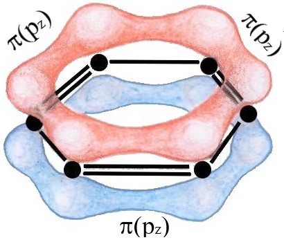
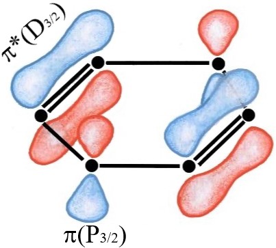
Figure 1: Graphene cell models with three dimers per hexagonal cell so that the electron density of the dimers overlaps (a) and with two conjugated double bonds and one ‘‘broken’’ $\pi$-bond (b) that $\pi$- and $\pi^{*}$-electrons are on terms $P_{3/2}$ and $D_{3/2}$ with a total angular momentum $J=3/2$. The equality of $P_{3/2}$- and $D_{3/2}$-terms energies in the case of relativistic hydrogen-like atom provides stability of configurations with two dimers.

The high-energy $\vec{k}\cdot\vec{p}$ Hamiltonian of a quasiparticle in the sublattice, for example, $A$ reads our-symmetry2020

$$\left[\vec{\sigma}\cdot\vec{p}+\vec{\sigma}\cdot\hbar\left(\vec{K}_{B}-\vec{K}_{A}\right)\right]\left|\psi^{*}_{BA}\right>-{i^{2}\over c}\Sigma_{AB}\Sigma_{BA}\widehat{\psi}^{\dagger}_{-\sigma_{A}}\left|0,-\sigma\right>=E_{qu}\widehat{\psi}^{\dagger}_{-\sigma_{A}}\left|0,-\sigma\right>,$$ (2)

$$\left|\psi^{*}_{BA}\right>=\Sigma_{BA}\widehat{\psi}^{\dagger}_{-\sigma_{A}}\left|0,-\sigma\right>\ \ \$$ (3)

where $\widehat{\psi}^{\dagger}_{-\sigma_{A}}\left|0,-\sigma\right>$ is a spinor wave function (vector in the Hilbert space), $\vec{\sigma}=\{\sigma_{x},\sigma_{y}\}$ is the 2D vector of the Pauli matrixes, $\vec{p}=\{p_{x},p_{y}\}$ is the 2D momentum operator, $\Sigma_{AB}$, $\Sigma_{BA}$ are relativistic exchange operators for sublattices $A,B$ respectively; $i^{2}\Sigma_{AB}\Sigma_{BA}$ is an unconventional Majorana-like mass term for a quasiparticle in the sublattice $A$, $\left|\psi^{*}_{BA}\right>$ is a spinor wave function of quasiparticle in the sublattice $B$, $\vec{K}_{A}(\vec{K}_{B})$ denote the graphene Dirac point (valley) $\vec{K}$($\vec{K}^{\prime}$) in the Brillouin zone, $\hbar=h/(2\pi)$, $h$ is the Planck constant. A small term $\hbar\vec{\sigma}\cdot\left(\vec{K}_{B}-\vec{K}_{A}\right)\sim{\frac{h}{a}}$ in Eq. (2) is a spin–valley-current coupling. One can see that the term with the conventional Dirac mass in (2) is absent. Since the exchange operators transform a wave function from sublattice $A$ into $B$ and visa versa in accord with Eq.(3) the following expression holds

$$\begin{split}\left|\tilde{\psi}^{*}_{BA}\right\rangle=\Sigma_{BA}\Sigma_{AB}\Sigma_{BA}\left|\psi_{A}\right\rangle=\Sigma_{BA}^{2}\Sigma_{AB}\psi_{A}+\Sigma_{BA}[\Sigma_{AB},\Sigma_{BA}]\left|\psi_{A}\right\rangle\\ =\Sigma_{BA}^{2}\{\Sigma_{AB}+\Sigma_{BA}^{-1}[\Sigma_{AB},\Sigma_{BA}]\}\left|\psi_{A}\right\rangle.\end{split}$$

Since the latter can be written in a form $\left|\tilde{\psi}^{*}_{BA}\right\rangle=\Sigma_{BA}^{2}\left|\tilde{\psi}_{A}\right\rangle$ one gets the following property of the exchange operator matrix:

$$\left|\tilde{\psi}^{*}_{BA}\right\rangle\equiv\alpha^{-1}\Sigma_{BA}\left|\tilde{\psi}_{A}\right\rangle=\Sigma_{BA}^{2}\left|\tilde{\psi}_{A}\right\rangle,$$ (4)

with some parameter $\alpha$. Due to the property (4), $\Sigma_{BA}\left(\Sigma_{BA}\hat{\psi}^{\dagger}_{-\sigma_{A}}\right)={\frac{1}{\alpha}}\Sigma_{BA}\hat{\psi}^{\dagger}_{-\sigma_{A}}$ and by the following notations

$$\vec{\sigma}_{AB}=\Sigma_{BA}\vec{\sigma}\Sigma^{-1}_{BA},\ \vec{p}_{BA}=\Sigma_{BA}\,\vec{p}\,\Sigma^{-1}_{BA},\ \vec{K}^{BA}_{B}-\vec{K}^{BA}_{A}=\Sigma_{BA}(\vec{K}_{B}-\vec{K}_{A})\Sigma^{-1}_{BA},$$ (5)

$$M_{BA}=i^{2}\alpha\Sigma_{BA}\Sigma_{AB},\ M_{AB}=i^{2}\alpha\Sigma_{AB}\Sigma_{BA}.$$ (6)

Eq. (3) can be rewritten as

$$\left[\vec{\sigma}_{AB}\cdot\left(\vec{p}_{BA}+\hbar(\vec{K}^{BA}_{B}-\vec{K}^{BA}_{A})\right)-{\frac{1}{c}}M_{BA}\right]\Sigma_{BA}\hat{\psi}^{\dagger}_{-\sigma_{A}}\left|0,-\sigma\right>=\hat{v}_{F}^{-1}E_{qu}\Sigma_{BA}\hat{\psi}^{\dagger}_{-\sigma_{A}}\left|0,-\sigma\right>.$$ (7)

The equation similar to (7), can be also written for the sublattice $B$. As a result, one gets the equations of motion for a Majorana bispinor $(\left|\psi_{AB}\right\rangle,\left|\psi^{*}_{BA}\right\rangle)^{T}$ Grush-KrylSymmetry2016 ; myNPCS18-2015 :

$$\left[\vec{\sigma}_{2D}^{BA}\cdot\vec{p}_{AB}-c^{-1}M_{AB}\right]\left|\psi_{AB}\right\rangle=i{\frac{\partial}{\partial t}}\left|\psi^{*}_{BA}\right\rangle,$$ (8)

$$\left[\vec{\sigma}_{2D}^{AB}\cdot\vec{p}\,^{*}_{BA}-c^{-1}\left(M_{BA}\right)^{*}\right]\left|\psi_{BA}\right\rangle=-i{\frac{\partial}{\partial t}}\left|\psi^{*}_{AB}\right\rangle.\quad$$ (9)

Then, the exchange interaction term $\Sigma_{rel}^{x}$ is determined as NPCS18-2015GrushevskayaKrylovGaisyonokSerow

$$\Sigma_{rel}^{x}\left(\begin{array}[]{c}\widehat{\chi}^{\dagger}_{{}_{-\sigma_{{}_{A}}}}(\vec{r})\\ \widehat{\chi}^{\dagger}_{\sigma_{{}_{B}}}(\vec{r})\end{array}\right)\left|0,-\sigma\right>\left|0,\sigma\right>=\left(\begin{array}[]{cc}0&\Sigma_{AB}\\ \Sigma_{BA}&0\end{array}\right)\left(\begin{array}[]{c}\widehat{\chi}^{\dagger}_{-\sigma_{{}_{A}}}(\vec{r})\\ \widehat{\chi}^{\dagger}_{\sigma_{{}_{B}}}(\vec{r})\end{array}\right)\left|0,-\sigma\right>\left|0,\sigma\right>,$$ (16)

$$\Sigma_{AB}\widehat{\chi}^{\dagger}_{\sigma_{{}_{B}}}(\vec{r})\left|0,\sigma\right>$$

$$=\sum_{i=1}^{N_{v}\,N_{c}}\int{d\vec{r}_{i}}\widehat{\chi}^{\dagger}_{\sigma_{i}{{}^{B}}}(\vec{r})\left|0,\sigma\right>\Delta_{AB}\langle 0,-\sigma_{i}|{\widehat{\chi}}^{\dagger}_{-\sigma_{i}^{A}}(\vec{r}_{i})V(\vec{r}_{i}-\vec{r}){\widehat{\chi}}_{-\sigma_{B}}(\vec{r}_{i})|0,-\sigma_{i^{\prime}}\rangle,\ \$$ (17)

$$\Sigma_{BA}\widehat{\chi}^{\dagger}_{{}_{-\sigma_{{}_{A}}}}(\vec{r})\left|0,-\sigma\right>$$

$$=\sum_{i^{\prime}=1}^{N_{v}\,N_{c}}\int{d\vec{r}_{i^{\prime}}}\widehat{\chi}^{\dagger}_{{}_{-\sigma_{i^{\prime}}^{A}}}(\vec{r})\left|0,-\sigma\right>\Delta_{BA}\langle 0,\sigma_{i^{\prime}}|{\widehat{\chi}}^{\dagger}_{\sigma_{i^{\prime}}^{B}}(\vec{r}_{i^{\prime}})V(\vec{r}_{i^{\prime}}-\vec{r}){\widehat{\chi}}_{{}_{\sigma_{A}}}(\vec{r}_{i^{\prime}})|0,\sigma_{i}\rangle.\ \$$ (18)

Here $N_{v}$ and $N_{c}$ are a number of valent electrons in one primitive-lattice cell and a number of the cells; interaction ($2\times 2$)-matrices $\Delta_{AB}$ and $\Delta_{BA}$ are gauge fields (or components of a gauge field). In the case of the basic set (1), vector-potentials for these gauge fields are determined by the phases $\alpha_{0}$ and $\alpha_{\pm,k}$, $k=1,\ 2,\ 3$ of wave functions $\psi_{\mbox{\small p}_{z}}(\vec{r})$ and $\psi_{\mbox{\small p}_{z},\pm\vec{\delta}_{k}}(\vec{r})$, $k=1,\ 2,\ 3$ respectively that the exchange interaction $\Sigma_{rel}^{x}$ (16) in accounting of the nearest lattice neighbours for a tight-binding approximation reads Taylor2016 ; myNPCS18-2015 ; NPCS18-2015GrushevskayaKrylovGaisyonokSerow

$$\Sigma_{AB}={\frac{1}{\sqrt{2}(2\pi)^{3}}}e^{-\imath(\theta_{k_{A}}-\theta_{K_{B}})}\sum_{i=1}^{3}\exp\{\imath[\vec{K}^{i}_{A}-\vec{q}_{i}]\cdot\vec{\delta}_{i}\}\int V(\vec{r})d{\vec{r}}$$

$$\times\left(\begin{array}[]{cc}\sqrt{2}\psi_{\mbox{\small p}_{z}}(\vec{r})\psi^{*}_{\mbox{\small p}_{z},-\vec{\delta}_{i}}(\vec{r})&\psi_{\mbox{\small p}_{z}}(\vec{r})[\psi^{*}_{\mbox{\small p}_{z}}(\vec{r})+\psi^{*}_{\mbox{\small p}_{z},-\vec{\delta}_{i}}(\vec{r})]\\ \psi^{*}_{\mbox{\small p}_{z},-\vec{\delta}_{i}}(\vec{r})[\psi_{\mbox{\small p}_{z},\vec{\delta}_{i}}(\vec{r})+\psi_{\mbox{\small p}_{z}}(\vec{r})]&{[\psi_{\mbox{\small p}_{z},\vec{\delta}_{i}}(\vec{r})+\psi_{\mbox{\small p}_{z}}(\vec{r})][\psi^{*}_{\mbox{\small p}_{z}}(\vec{r})+\psi^{*}_{\mbox{\small p}_{z},-\vec{\delta}_{i}}(\vec{r})]\over\sqrt{2}}\end{array}\right),$$ (21)

$$\Sigma_{BA}={1\over\sqrt{2}(2\pi)^{3}}e^{-\imath(\theta_{K_{A}}-\theta_{K_{B}})}\sum_{i=1}^{3}\exp\{\imath[\vec{K}^{i}_{A}-\vec{q}_{i}]\cdot\vec{\delta}_{i}\}\int V(\vec{r})d{\vec{r}}$$

$$\times\left(\begin{array}[]{cc}{[\psi_{\mbox{\small p}_{z},\vec{\delta}_{i}}(\vec{r})+\psi_{\mbox{\small p}_{z}}(\vec{r})][\psi^{*}_{\mbox{\small p}_{z}}(\vec{r})+\psi^{*}_{\mbox{\small p}_{z},-\vec{\delta}_{i}}(\vec{r})]\over\sqrt{2}}&-\psi^{*}_{\mbox{\small p}_{z},-\vec{\delta}_{i}}(\vec{r})[\psi_{\mbox{\small p}_{z},\vec{\delta}_{i}}(\vec{r})+\psi_{\mbox{\small p}_{z}}(\vec{r})]\\ -\psi_{\mbox{\small p}_{z}}(\vec{r})[\psi^{*}_{\mbox{\small p}_{z}}(\vec{r})+\psi^{*}_{\mbox{\small p}_{z},-\vec{\delta}_{i}}(\vec{r})]&\sqrt{2}\psi_{\mbox{\small p}_{z}}(\vec{r})\psi^{*}_{\mbox{\small p}_{z},-\vec{\delta}_{i}}(\vec{r})\end{array}\right)$$ (24)

where the origin of the reference frame is located at a given site on the sublattice $A$($B$), $V(\vec{r})$ is the 3D Coulomb potential, designations $\psi_{\mbox{\small p}_{z},\ \pm\vec{\delta}_{i}}(\vec{r})$, $\psi_{\mbox{\small p}_{z},\ \pm\vec{\delta}_{i}}(\vec{r}_{2D})\equiv\psi_{\mbox{\small p}_{z}}(\vec{r}\pm\vec{\delta}_{i})$, $i=1,2,3$ refer to atomic orbitals of p_z-electrons with 3D radius-vectors $\vec{r}\pm\vec{\delta}_{i}$ in the neighbor lattice sites $\vec{\delta}_{i}$, nearest to the reference site ; $\vec{r}\pm\vec{\delta}_{i}$ is the p_z-electron 3D-radius-vector. Elements of the matrices $\Sigma_{AB}$ and $\Sigma_{BA}$ include bilinear combinations of the wave functions so that their phases $\alpha_{0}$ and $\alpha_{\pm,k}$, $k=1,\ 2,\ 3$ enter into $\Delta_{AB}$ and $\Delta_{BA}$ from (17 and 18) in the form

$$\left|\psi_{\mbox{\small p}_{z}}\right|\left|\psi_{\mbox{\small p}_{z},\ \pm\vec{\delta}_{k}}\right|\exp\left\{\imath\left(\alpha_{0}-\alpha_{\pm,k}\right)\right\}\equiv\left|\psi_{\mbox{\small p}_{z}}\right|\left|\psi_{\mbox{\small p}_{z},\ \pm\vec{\delta}_{k}}\right|\Delta_{\pm,k}.$$ (25)

Due to the fact that phases are included into (15) only with their differences, an effective number $N_{F}$ of flavors in our gauge field theory is equal to 3, separately for holes and electrons (signs plus and minus in (15) refer to hole and electrons, respectively). Then owing to translational symmetry we determine the gauge fields $\Delta_{\pm,i}$ in Eq. (25) in the following form:

$$\Delta_{\pm,i}(q)=\exp\left(\pm\imath c_{\pm}(q)({\vec{q}}\cdot{\vec{\delta}_{i}})\right).$$ (26)

Substituting the relative phases (26) of particles and holes into (21) one gets the exchange interaction operator $\Sigma_{AB}$

$$\Sigma_{AB}={1\over\sqrt{2}(2\pi)^{3}}e^{-\imath(\theta_{k_{A}}-\theta_{K_{B}})}\left(\begin{array}[]{cc}\Sigma_{11}&\Sigma_{12}\\ \Sigma_{21}&\Sigma_{22}\end{array}\right)$$ (29)

with the following matrix elements:

$$\Sigma_{11}=\sqrt{2}\left\{\sum_{j}I_{11}^{j}\Delta_{-,j}(q)\exp\{\imath[\vec{K}^{j}_{A}-\vec{q}]\cdot\vec{\delta}_{j}\}\right\},$$

$$\Sigma_{12}=\left\{\sum_{j}\left(I_{12}^{j}+I_{11}^{j}\Delta_{-,j}(q)\right)\exp\{\imath[\vec{K}^{j}_{A}-\vec{q}]\cdot\vec{\delta}_{j}\}\right\},$$

$$\Sigma_{21}=\left\{\sum_{j}\left(I_{21}^{j}\Delta_{+,j}(q)\Delta_{-,j}(q)+I_{11}^{j}\Delta_{-,j}(q)\right)\exp\{\imath[\vec{K}^{j}_{A}-\vec{q}]\cdot\vec{\delta}_{j}\}\right\},$$

$$\Sigma_{22}={1\over\sqrt{2}}\left\{\sum_{j}\left(I_{22}^{j}\Delta_{+,j}(q)+I_{12}^{j}+I_{21}^{j}\Delta_{+,j}(q)\Delta_{-,j}(q)+I_{11}^{j}\Delta_{-,j}(q)\right)\exp\{\imath[\vec{K}^{j}_{A}-\vec{q}]\cdot\vec{\delta}_{j}\}\right\}$$

where $I_{n_{i}m_{k}}^{j}=\int V(\vec{r})\psi_{\mbox{\small p}_{z}+n_{i}\vec{\delta}_{j}}{\psi^{*}}_{\mbox{\small p}_{z}-m_{k}\vec{\delta}_{j}}\ d\vec{r}$, $i,k=1,2$; $(n_{1},m_{1})=(0,1)$, $(n_{1},m_{2})=(0,0)$, $(n_{2},m_{1})=(n_{2},m_{2})=(1,1)$. There are similar formulas for $\Sigma_{BA}$.

Accordingly to (26) eigenvalues $E_{i},\ i=1,\ldots,4$ of the $4\times 4$ Hamiltonian (8, 9) are functionals of $c_{\pm}$. To eliminate arbitrariness in the choice of the phase factors $c_{\pm}$ one needs a gauge condition for the gauge fields. The eigenvalues $E_{i},\ i=1,\ldots,4$ are real because the system of equations (8, 9) can be transformed to Klein–Gordon–Fock equation Grush-KrylSymmetry2016 . Therefore we impose the gauge condition as a requirement on the absence of imaginary parts in the eigenvalues $E_{i},\ i=1,\ldots,4$ of the Hamiltonian (8, 9):

$$\Im m(E_{i})=0,\ i=1,\ldots,4.$$ (30)

To satisfy the condition (30) in the momentum space we minimize the function $f(c_{+},c_{-})=\sum_{i=1}^{4}\left|\Im m\ E_{i}\right|$ absolute minimum of which coincides with the solution of the system (30). The bandstructures determined by the sublattice Hamiltonians without the pseudo-Majorana mass term are the same. Therefore when neglecting the pseudo-Majorana mass term, one can choose the cost function $f={2}\sum_{i=1}^{2}\left|\Im m\ E_{i}\right|$. For the non-zero mass case, we assume the same form of the function $f$ due to the smallness of the mass correction.

II.2 Non-Abelian-Zak-phase analysis of emerging polarization

Topological defect pushes out a charge carrier from its location. The operator of this non-zero displacement presents a projected position operator ${\cal P}{\vec{r}}{\cal P}$ with the projection operator ${\cal P}=\sum_{n=1}^{N_{B}}\left|\psi_{n,\vec{k}}\right\rangle\left\langle\psi_{n,\vec{k}}\right|$ for the occupied subspace of states $\psi_{n,\vec{k}}(\vec{r})$. Here $N_{B}$ is a number of occupied bands, $\vec{k}$ is a momentum. Eigenvalues of ${\cal P}{\vec{r}}{\cal P}$ are called Zak phase Zak89 . The Zak phase coincides with a phase

$$\gamma_{mn}=i\int\limits_{C(\vec{k})}\left<\psi_{m,\vec{k}}\left|\nabla_{\vec{k}}\right|\psi_{n,\vec{k}}\right>\cdot d\vec{k},\quad n,m=1,\ldots,N_{B}$$ (31)

of a Wilson loop ${\cal W}^{mn}=\mbox{T }\exp(i\gamma_{mn})$ being a path-ordered (T) exponential with the integral over a closed contour $C(\vec{k})$ PhysRevX6-2016Muechler . We discretize the Wilson loop by Wilson lines ${\cal W}^{mn}_{k_{i+1},k_{i}}$ our-symmetry2020 :

$${\cal W}^{mn}=\prod_{i=0}^{N_{\cal W}\to\infty}{\cal W}^{mn}_{\vec{k}_{i+1},\vec{k}_{i}}=\prod_{i=0}^{N_{\cal W}\to\infty}\left\langle\psi^{*}_{m,\vec{k}_{i+1}}\left|\right.\psi_{n,\vec{k}_{i}}\right\rangle.$$ (32)

Here momenta $\vec{k}_{i}$, $i=0,1,\ldots,N_{\cal W}$ form a sequence of the points on a curve (ordered path), connecting initial and final points in the Brillouin zone: $\vec{k}_{i}=\vec{k}_{0}+\sum_{j=1}^{i}\Delta\vec{k}_{j,j-1}$, $\Delta\vec{k}_{j,j-1}=\vec{k}_{j}-\vec{k}_{j-1}\to 0$ and $\vec{k}_{N_{\cal W}}=\vec{k}_{0}$; $\psi_{n,{\vec{k}_{i}}}$, $n=1,\ldots,N_{B}$ are eigenstates of a model Hamiltonian.

We consider the parallel transport of filled Bloch waves around momentum loops $\vec{l}$ because the basis of Wannier functions generated only by the occupied Bloch eigenstates. Global characterization of all Dirac touching is possible with a non-Abelian Zak invariant defined over a non-contractible momentum loop Zak89 . Therefore, instead of the closed contour, we take a curve $C(\vec{k})$ being one side $\vec{l}(k_{y})$ of the equilateral triangle of variable size (defined by the value of $k_{y}$ component of the wavevector $\vec{k}$) with the coordinate-system origin in the Dirac $K(K^{\prime})$-point. The $N_{B}$ phases are defined then as arguments of the eigenvalues of the Wilson loop. One chooses $N_{\cal W}$ ($N_{\cal W}=500$) that a ‘‘noise’’ in output data is sufficiently small to observe the discrete values of Zak phases. In our calculation of (32) for the Hamiltonian without the pseudo-Majorana mass term, a number $N_{B}$ of bands is equal to four ($N_{B}=4$): two electron and hole valent bands and two electron and hole conduction bands (see simulation results in Section 2.1).

II.3 Non-Abelian currents in quasi-relativistic graphene model

Conductivity can be considered as a coefficient linking the current density with an applied electric field in a linear regime of response. To reach the goal, several steps should be performed. First, one has to subject the system to an electromagnetic field, this can be implemented by standard change to canonical momentum $\vec{p}\to\vec{p}-{e\over c}\vec{A}$ in the Hamiltonian where $\vec{A}$ is a vector-potential of the field, $e$ is the electron charge. Then, one can find a quasi-relativistic current Davydov of charge carriers in graphene as:

$$j_{i}^{SM}=c^{-1}j_{i}\equiv j_{i}^{O}+j_{i}^{Zb}+j_{i}^{so},$$

$$j_{i}=e\chi^{\dagger}_{+\sigma_{{}_{B}}}(x^{+})v^{i}_{x^{+}x^{-}}\chi_{+\sigma_{{}_{B}}}(x^{-})-{e^{2}A_{i}\over c\,M_{AB}}\chi_{+\sigma_{{}_{B}}}^{\dagger}(x^{+})\chi_{+\sigma_{{}_{B}}}(x^{-})$$

$$+{e\hbar\over 2M_{AB}}\left[\vec{\nabla}\times\chi_{+\sigma_{{}_{B}}}^{\dagger}(x^{+})\vec{\sigma}\chi_{+\sigma_{{}_{B}}}(x^{-})\right]_{i},\ i=1,2.$$ (33)

Here

$$x^{\pm}=x\pm\epsilon,\ x=\{\vec{r},\ t_{0}\},\ \vec{r}=\{x,y\},\ t_{0}=0,\ \epsilon\to 0;$$ (34)

$v^{i}_{x^{+}x^{-}}$ is the velocity operator determined by a derivative of the Hamiltonian (8,9), $\chi_{+\sigma_{{}_{B}}}(x^{+})$ is the secondary quantized fermion field, the terms $j_{i}^{O},\ j_{i}^{Zb},\ j_{i}^{so}$, $i=x,y$ describe an ohmic contribution which satisfies the Ohm law and contributions of the polarization and magneto-electric effects respectively. A potential-energy operator $V$ for interaction between the secondary quantized fermionic field $\chi_{+\sigma_{{}_{B}}}(x)$ with an electromagnetic field reads

$$V=\chi^{\dagger}_{+\sigma_{{}_{B}}}\left[-c\vec{\sigma}_{BA}\cdot{e\over c}\vec{A}-M_{BA}(0)-\sum_{i}\left.{dM_{BA}\over dp_{i}^{\prime}}\right|_{p_{i}^{\prime}=0}\right.$$

$$\times\left(p_{i}^{AB}-{e\over c}A_{i}\right)-{1\over 2}\sum_{i,j}\left.{d^{2}M_{BA}\over dp_{i}^{\prime}dp_{j}^{\prime}}\right|_{p_{i}^{\prime},\ p_{j}^{\prime}=0}\left.\left(p_{i}^{AB}-{e\over c}A_{i}\right)\,\left(p_{j}^{AB}-{e\over c}A_{j}\right)+\ldots\right]\chi_{+\sigma_{{}_{B}}}.$$ (35)

To perform quantum-statistical averaging for the case of non-zero temperature, we use a quantum field method developed in Varlamov ; myConductivity . After tedious but simple algebra one can find the conductivity in our model:

$$\sigma_{ii}^{O}(\omega,\ k)={\imath e^{2}\bar{\beta}^{2}\over(2\pi c)^{2}}\mbox{Tr}\ \int\left(1-M_{BA}(\vec{p}){\partial^{2}M_{BA}\over\partial p_{i}^{2}}\right)\left(M\vec{v}^{i}(p)\,,\,N\vec{v}^{i}(p)\right)\,d\vec{p},$$ (36)

$$\sigma_{ll}^{Zb}(\omega,k)={\imath e^{2}\bar{\beta}^{2}\over(2\pi c)^{2}}\mbox{Tr }\ \int{M_{BA}(\vec{p})\over 2}\sum_{i=1}^{2}{\partial^{2}M_{BA}\over\partial p_{i}^{2}}\left(M\vec{v}^{i}(p)\,,\,N\vec{v}^{i}(p)\right)\,d\vec{p},$$ (37)

$$\sigma_{12(21)}^{so}(\omega,k)={(-1)^{1(2)}\imath\over 2}{\imath e^{2}\bar{\beta}^{2}\over(2\pi c)^{2}}\mbox{Tr }\ \int{M_{BA}(\vec{p})}{\partial^{2}M_{BA}\over\partial p_{1}\partial p_{2}}\left(M\vec{v}\,^{1(2)}(p)\,,\,N\vec{v}\,^{1(2)}(p)\right)\sigma_{z}d\vec{p}$$ (38)

for the currents $j_{i}^{O},\ j_{i}^{Zb},\ j_{i}^{so}$ respectively. Here the matrices $M,\ N$ are given by the following expressions:

$$M={f[\bar{\beta}((H(p^{+})-\mu)/\hbar)]-f[\bar{\beta}(H^{\dagger}(-p^{-})-\mu/\hbar)]\over\bar{\beta}z-\bar{\beta}(H(p^{+})/\hbar)+\bar{\beta}(H^{\dagger}(-p^{-})/\hbar)},\ N={\delta\left(\hbar\omega+\mu\right)\over(\hbar z+H(p^{+})-H^{\dagger}(-p^{-}))\bar{\beta}}.$$

Here $f$ is the Fermi–Dirac distribution, $z=\omega+i\epsilon$, $\vec{p}^{\pm}=\vec{p}\pm\vec{k}$, $\omega$ is a frequency, $\mu$ is a chemical potential, $\bar{\beta}$ is an inverse temperature divided by $c$.

III Results and discussion

III.1 Band structure simulations

The band structure of graphene within the quasi-relativistic $N_{F}=3$-flavors model has been calculated with the Majorana-like mass term and is presented in Fig. 2a. The graphene bands are conical near the Dirac point at $q(q^{\prime})\to 0$, $q=\left|\vec{p}-\vec{K}\right|$ ($q^{\prime}=\left|\vec{p}\;\!^{\prime}-\vec{K}^{\prime}\right|$) where $\vec{p}(\vec{p}\;\!^{\prime})$ is a momentum of electron (hole). But, they flatten at large $q(q^{\prime})$.

(a)

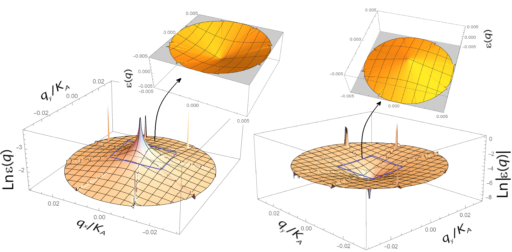
(b)

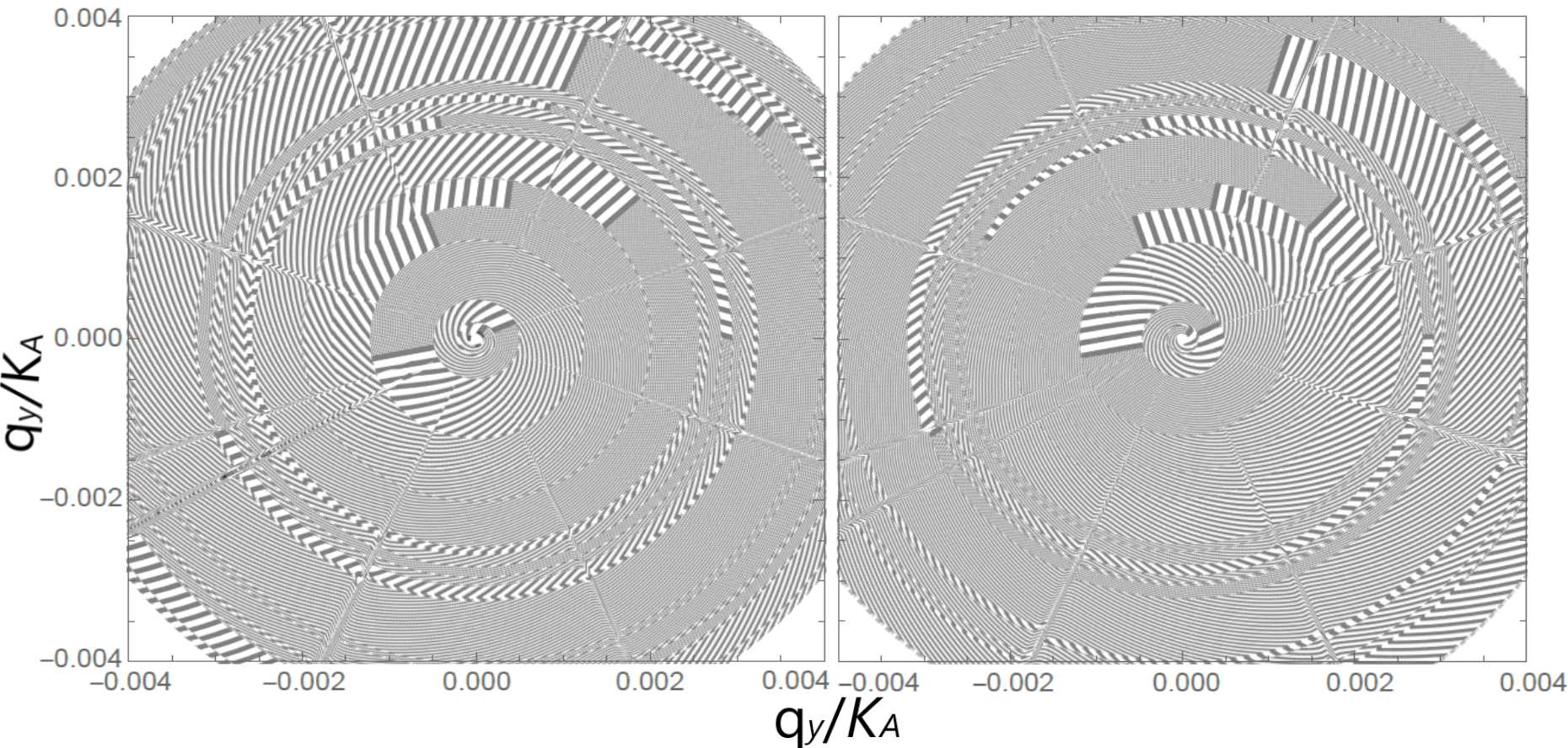
Figure 2: (a) Electron (left) and hole bands (right) of a quasi-relativistic $N_{F}=3$-flavors model graphene with a pseudo-Majorana mass term. (b) The vortex texture in contour plots of the graphene electron (left) and hole (right) bands.

The band structure of graphene within the quasirelativistic model with pseudo Majorana charge carriers hosts vortex and antivortex whose cores are in the graphene valleys $\vec{K}$ and $\vec{K}^{\prime}$ of the Brillouin zone, respectively (see Fig. 2b). Touching in the Dirac point $K(K^{\prime})$ the cone-shaped valence and conduction bands of graphene flatten at large momenta $p$ of the graphene charge carriers our-symmetry2020 . It signifies that the Fermi velocity $v_{F}$ diminishes drastically to very small values at large $p$. Since eight sub-replicas of the graphene band near the Dirac point degenerate into the eight-fold conic band (see Fig. 2) the pseudo Majorana fermions forming the eightfold degenerate vortex are confined by the hexagonal symmetry. In the state of confinement, the pseudo Majorana fermions are linked with the formation of electron–hole pairs under the action of the hexagonal symmetry.

The non-Abelian Zak phases of the pseudo Majorana graphene charge carriers are nonzero our-symmetry2020 as it is shown in Fig. 3. The charge carriers, whose non-Abelian Zak phases are multiples of $\pi/6$ and constitute the cyclic groups $\mathbb{Z}_{12}$, are confined near the Dirac point. The $\pi/6$ rotation is equivalent to a $\pi/2$ rotation due to the hexagonal symmetry of graphene and, correspondingly, the electron and hole configurations in the momentum space are orthogonal to each other. It testifies the metallicity of zigzag edges and/or zigzag configurations and semi-conductivity of armchair edges and/or armchair configurations transversal to the zigzag configuration in the graphene plane. All $\pi(\mbox{p}_{z})$-electrons are precessed (move from one valley to another one) in a same way near the Dirac point because the hexagonal symmetry levels the transitions between the levels with different projections $j=\pm 3/2,\pm 1/2$ of the $\pi(\mbox{p}_{z})$-electron orbital momentum $J_{\mbox{p}_{z}}$ due to smallness of a spin-orbital coupling at momenta $q(q^{\prime})\to 0$, $\vec{q}=\vec{p}-\vec{K}$ ($\vec{q}\;\!^{\prime}=\vec{p}\;\!^{\prime}-\vec{K}^{\prime}$).

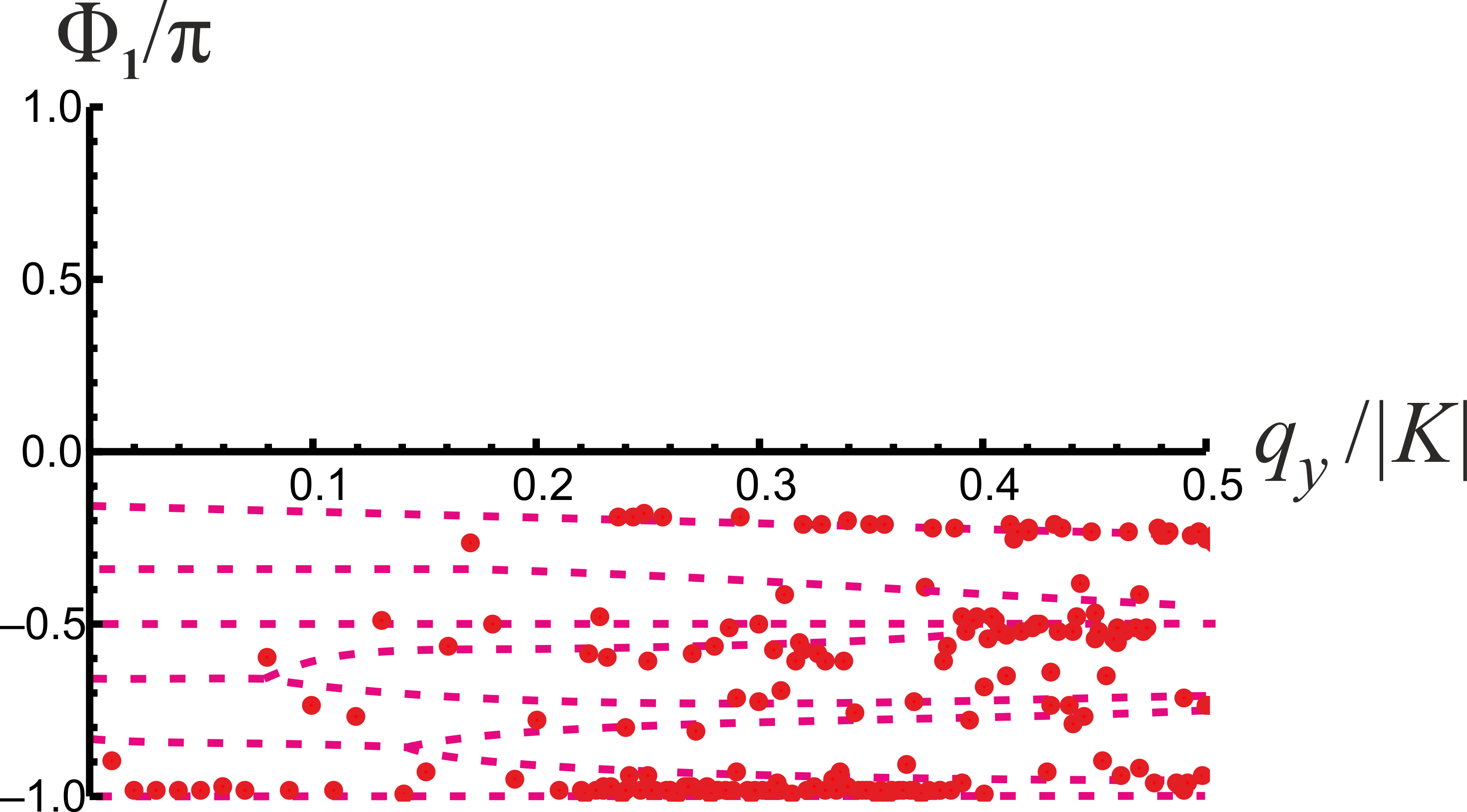
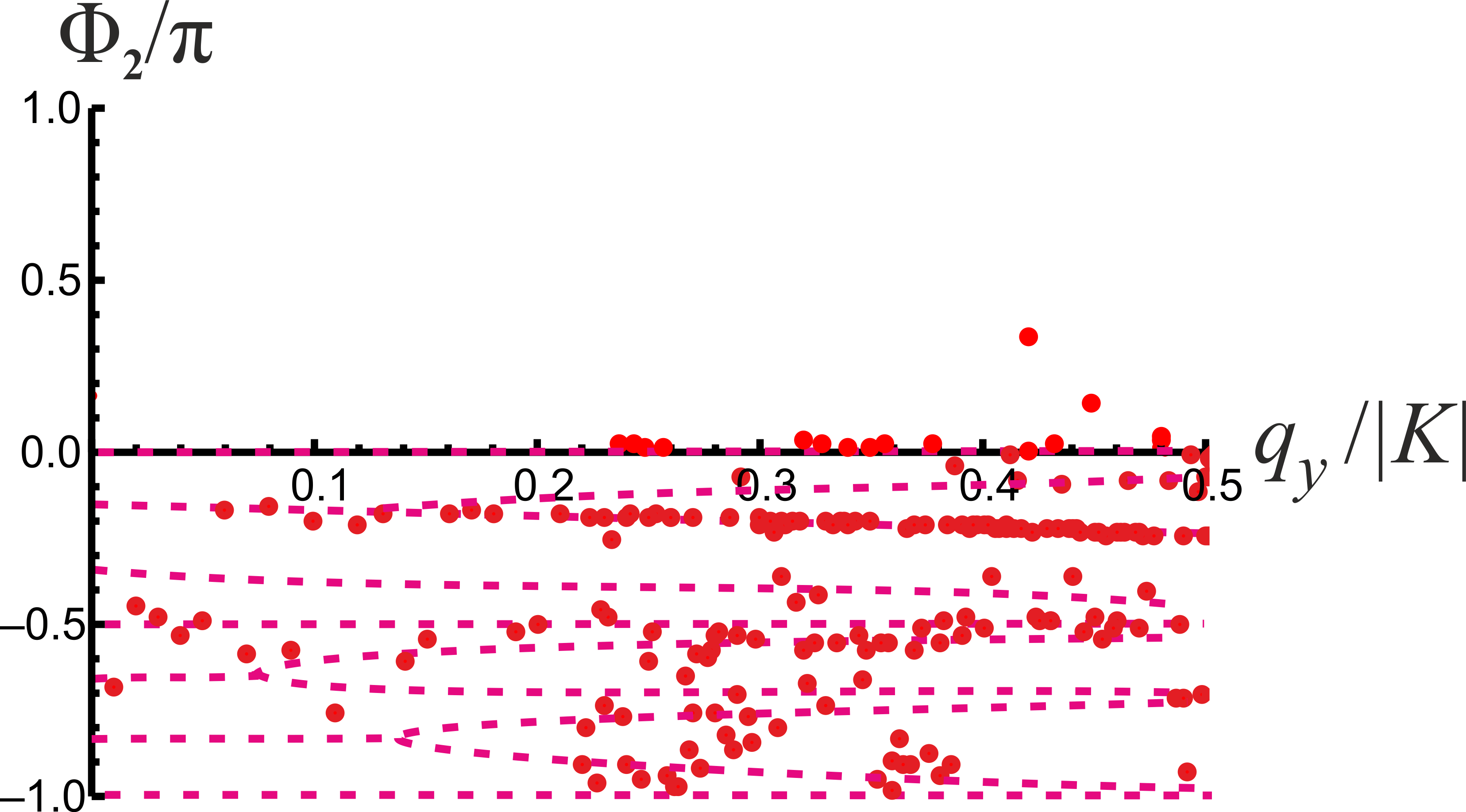
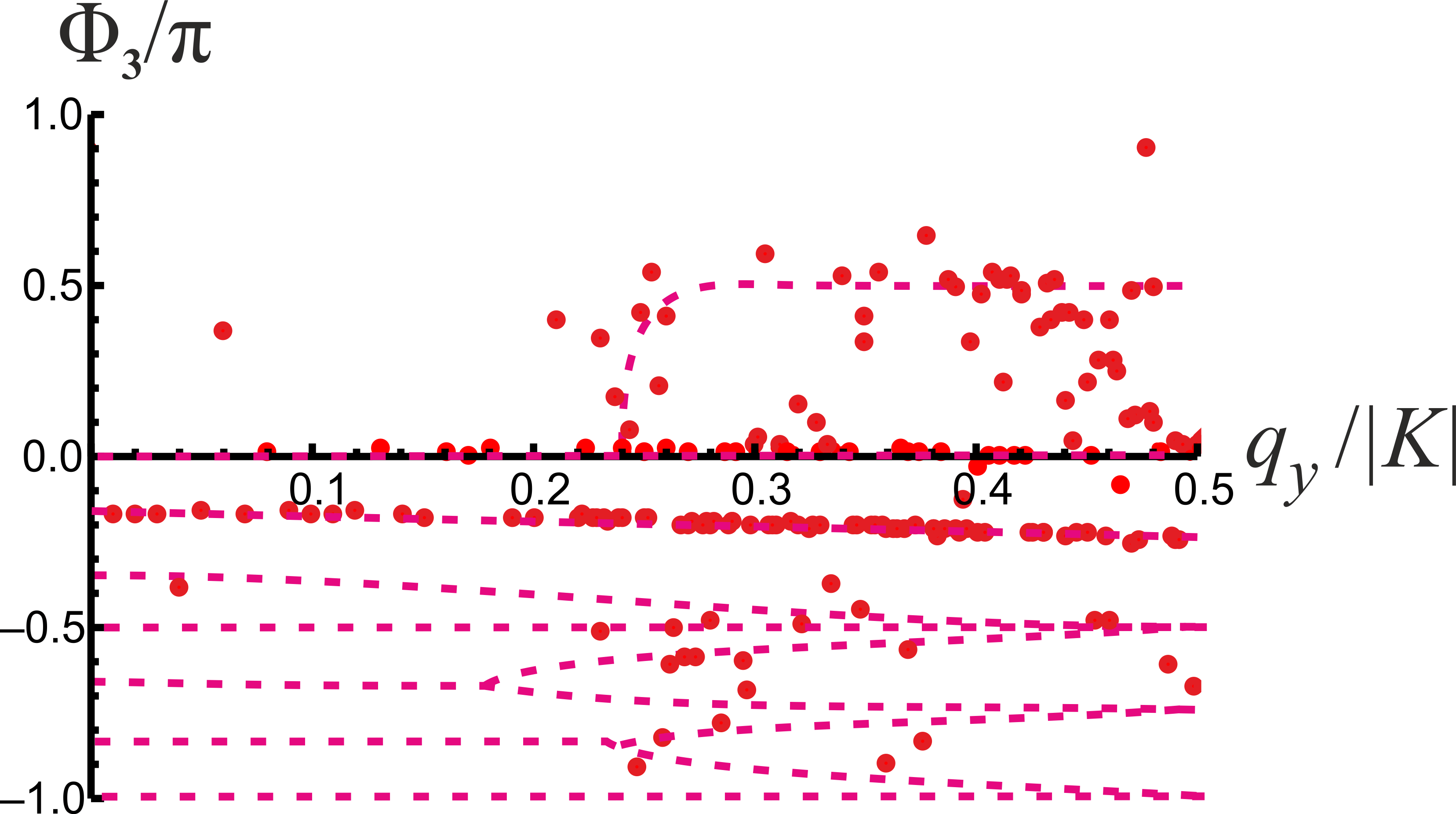
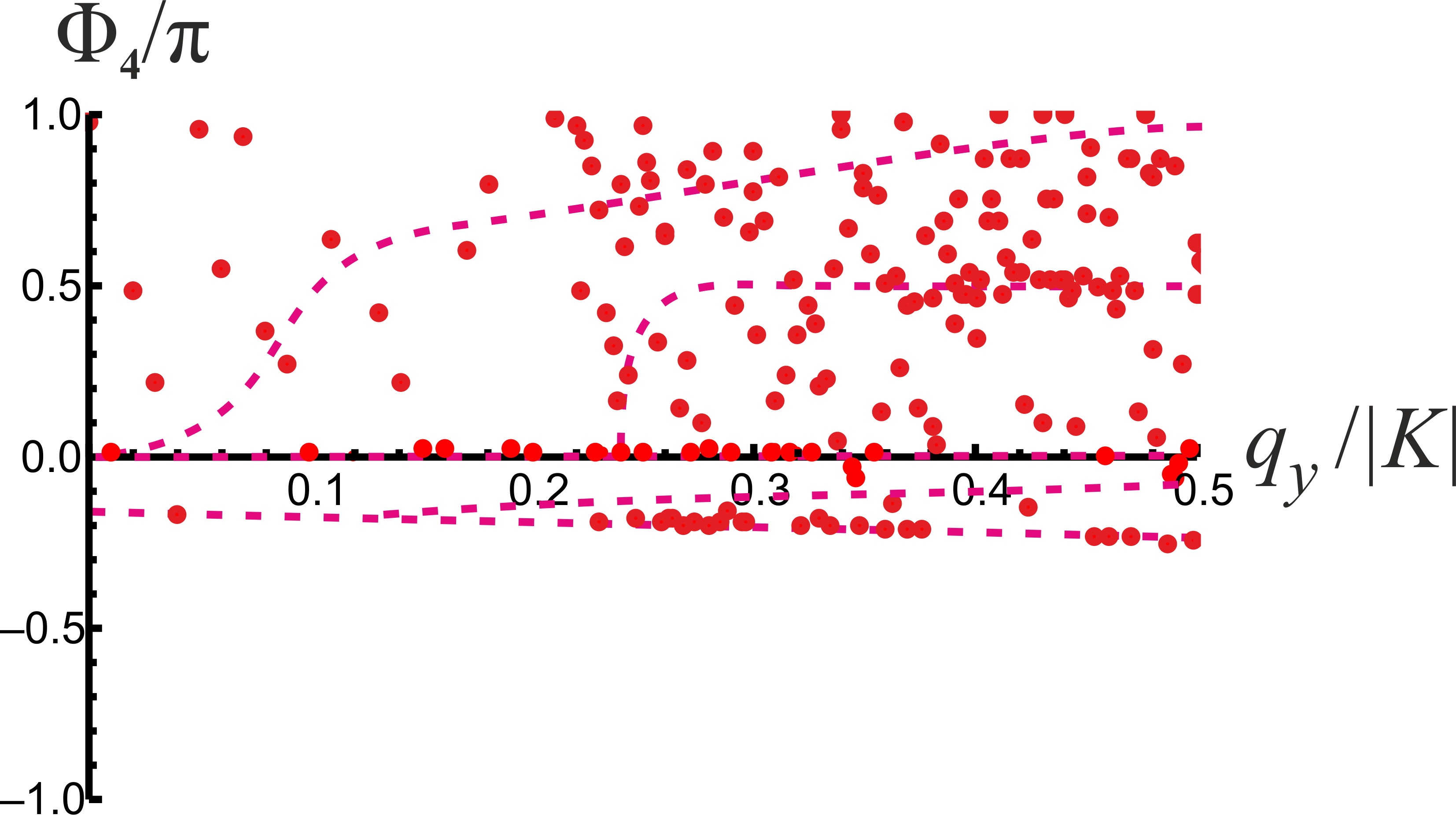
Figure 3: Non-Abelian phases $\Phi_{1},\ldots,\Phi_{4}$ of the Wilson-loop eigenvalues in the units of $\pi$ at non-zero gauge fields.

The strong spin-orbital coupling at large momenta $q(q^{\prime})$ violates the hexagonal symmetry lifting the degeneration over the projections $j$. The precessing of the $\pi(\mbox{p}_{z})$-electron proliferates vortices (antivortices) in the T-shaped configuration of four topological vortex defects (four antivortices) our-symmetry2020 . An atomic chain with two topological defects at the ends implements a pseudo Majorana particle Physics-Uspekhi44-2001Kitaev ; JPhysB40-2007Semenoff . Such T-shaped configuration of four topological vortex defects (four antivortices) is three pseudo Majorana quasiparticles differing in the combinations of vortex subreplicas that form them. The number of the pseudo Majorana modes coincides with the number of the gauge degrees of freedom ($N_{F}=3$) and, accordingly, all three Majorana modes differ in the flavor. It signifies that the pair of vortical and antivortical subreplicas holds one of three flavors.

A feature of the pseudo-Majorana mass term is its vanishing in the valleys $K(K)$. Outside the valleys one of two eigenvalues of the pseudo-Majorana mass term entering the Hamiltonian of the pseudo Majorana fermion turns out to be practically zero Grush-Kr2017. Therefore, one of the flavored Majorana particles is formed by two chiral vortex defects, the second one – by two nonchiral vortices, and only one of the two vortices is chiral for the third Majorana mode. Since the flavor is associated with a degree of chirality, let us call the pseudo Majorana flavor modes as the chiral, semichiral, and non-chiral pseudo Majorana quasiparticles $V_{ch},V_{sc},V_{nc}$.

The system of Eqs. (8, 9) for the stationary case can be approximated by a Dirac-like equation with the ‘‘Majorana-force‘‘ correction in the following way. The operator $\Sigma_{AB}^{-1}$ in (8) plays a role of Fermi velocity also: $\hat{v}^{\prime}_{F}=\Sigma_{AB}$. Then one can assume that there is the following expansion up to a normalization constant $\left<0\right|\hat{v}_{F}\left|0\right>=\left<0\right|\hat{v}^{\prime}_{F}\left|0\right>$:

$$\left|\psi_{AB}\right\rangle=\frac{\Sigma_{AB}\left|\psi^{*}_{BA}\right\rangle}{\left<0\right|\hat{v}^{\prime}_{F}\left|0\right>}=\frac{\Sigma_{AB}\Sigma_{BA}}{\left<0\right|\hat{v}^{\prime}_{F}\left|0\right>}\left|\psi_{AB}\right\rangle=\frac{\left\{\Sigma_{BA}+\left[\Sigma_{AB},\Sigma_{BA}\right]\right\}\left|\psi_{AB}\right\rangle}{\left<0\right|\hat{v}_{F}\left|0\right>}$$

$$\approx\left\{1+{\left(\Delta\Sigma+\left[\Sigma_{AB},\Sigma_{BA}\right]\right)\over\left<0\right|\hat{v}_{F}\left|0\right>}\right\}\left|\psi_{AB}\right\rangle$$ (39)

where $\left[\cdot,\cdot\right]$ denotes the commutator, $\Delta\Sigma=\Sigma_{BA}-\Sigma_{AB}$. Substituting (3, 39) into the right-hand side of the equation (9), one gets the Dirac-like equation with a ‘‘Majorana-force’’ correction of an order of quantum-exchanges difference for two graphene sublattices:

$$\left[\vec{\sigma}_{2D}^{AB}\cdot\vec{p}_{BA}-c^{-1}M_{BA}\right]\left|\psi^{*}_{BA}\right\rangle=\tilde{E}\left\{1+{\left(\Delta\Sigma+\left[\Sigma_{AB},\Sigma_{BA}\right]\right)\over\left<0\right|\hat{v}_{F}\left|0\right>}\right\}\left|\psi^{*}_{BA}\right\rangle$$ (40)

where $\tilde{E}=E/\left<0\right|\hat{v}_{F}\left|0\right>$. Now, neglecting the mass term, we can find the solution of the equation (40) by the successive approximation technique as:

$$\vec{\sigma}_{2D}^{BA}(\Delta_{\pm,i})\cdot\vec{p}_{AB}(\Delta_{\pm,i})\left|\psi_{AB}\right\rangle+{E^{(0)}\left(\Delta\Sigma(\Delta_{\pm,i})+\left[\Sigma_{AB}(\Delta_{\pm,i}),\Sigma_{BA}(\Delta_{\pm,i})\right]\right)\over\left<0|\hat{v}_{F}|0\right>^{2}}\left|\psi_{AB}\right\rangle$$

$$={E^{(1)}\over\hat{v}_{F}}\left|\psi_{AB}\right\rangle.$$ (41)

It follows from Eq. (41), that the quadratic correction describes a deconfinement of the pseudo Majorana fermions by SOC because the ‘‘Majorana-force‘‘ is significant in the flat regions of the graphene bands where the Fermi velocity trends to zero.

Thus, the pseudo Majorana fermion graphene model is a topological semimetal. Resulting in 8 subreplicas of the graphene band, the spin-orbital coupling is capable to compete with the hexagonal symmetry at high energies in the flat bands only. The pseudocubic symmetry signifies that the electron-hole symmetry of each graphene band is separately broken and, correspondingly, the associated vortex and antivortex Majorana fermions forming electrons and holes are released by strong SOC. These free Majorana particles exist in a very narrow energy range because they reside in the flat regions of the graphene bands. Since the Fermi velocity $v_{F}$ of the free Majorana configurations trends to zero, the pseudo Majorana fermions are very heavy ones.

III.2 Low-frequency dielectric permittivity of graphene

Let us investigate longitudinal conductivity for low frequencies $\omega\to 0$ and non-vanishing wave vectors $\vec{k}=\vec{p}/\hbar-\vec{K}_{A(B)}$. The longitudinal conductivity $\sigma_{L}(\omega,{\vec{k}})$ is determined through the conductivity tensor splitting into longitudinal and transversal terms as Kraft-Ropke

$$\sigma_{ij}(\omega,{\vec{k}})=\left(\delta_{ij}-\frac{k_{i}k_{j}}{{\vec{k}}^{2}}\right)\sigma_{T}(\omega,{\vec{k}})+\frac{k_{i}k_{j}}{{\vec{k}}^{2}}\sigma_{L}(\omega,{\vec{k}});i,j=x,y.$$ (42)

When choosing $\vec{k}=(k_{x},0)$ or $\vec{k}=(0,k_{y})$, $k_{x}=k_{y}=k$ one always has

$$\sigma_{xx}(\omega,{\vec{k}})=\sigma_{L}(\omega,k),\ \mbox{or}\ \sigma_{yy}(\omega,{\vec{k}})=\sigma_{L}(\omega,k).$$

Now let us calculate the low-frequency dielectric permittivity $\epsilon(\omega,\vec{r})$. To do it one has to perform the inverse Fourier transformation

$$\sigma(\omega,\vec{r})={1\over(2\pi)^{2}}\int{\sigma^{O}_{L}}(\omega,k)e^{i\vec{k}\cdot\vec{r}}d^{2}k$$ (43)

and then to substitute the transformation into the following expression:

$$\epsilon(\omega,\vec{r})=\Re e\left[1-4\pi\imath{\sigma(\omega,\vec{r})\over\omega}\right]=1+{4\pi\over\omega}\Im m\ \sigma(\omega,\vec{r}).$$ (44)

Here $\omega$ is a cyclic frequency. We consider the effects of spatial dispersion on the imaginary part $\Im m\ \sigma^{O}_{L}(\omega,k)$ of the longitudinal complex conductivity at the low frequencies: $\omega=10^{-10}$, $0.004$, 13.3 K (kelvin) for the massless pseudo Dirac graphene fermion model with the number of flavors $N_{F}=2$ (pseudospin and spirality) and our graphene model with the $N_{F}=3$ flavors. Conductivity for frequencies in Hertz range, for example, 2.08 Hz ($\omega=10^{-10}$ K) can be considered as a conductance for direct current. The numerical results are presented in Fig. 4 and Table 1.

(a)                                                                       (b)

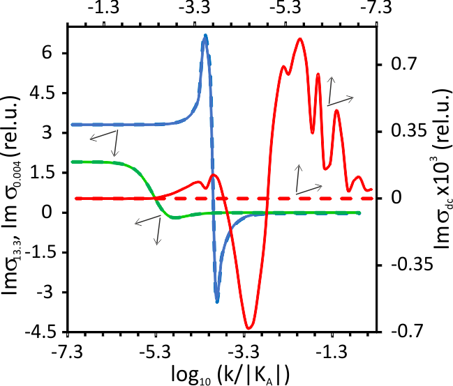
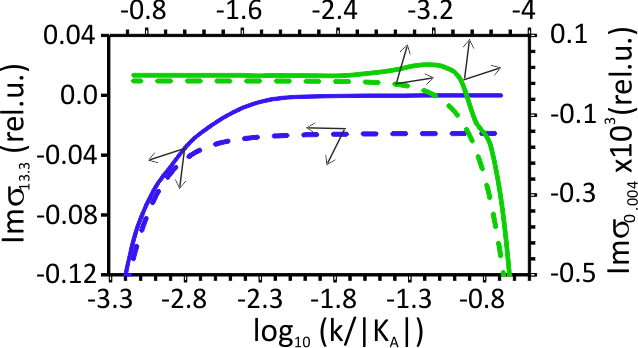
(c)                                                                       (d)

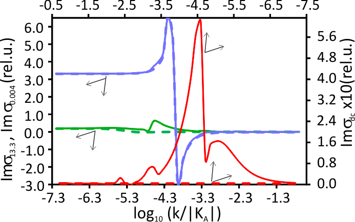
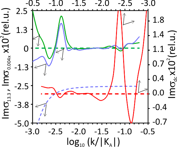
Figure 4: Imaginary part $\sigma_{L}^{O}(\omega,k)$ of longitudinal ohmic contribution to conductivity vs wave number $k$, $\vec{k}=\vec{p}-\vec{K}_{A(B)}$ for our pseudo Majorana fermion $N_{F}=3$-model (8),(9) without (a,b) and with (c,d) the pseudo-Majorana mass term (solid curves) and for the massless Dirac fermion model Varlamov (dashed curves), at the temperature 100 K and the frequencies $\omega$: $13.3$ K ($0.27$ THz, blue color), $0.004$ K ($83$ MHz, green color), $10^{-10}$ K ($2.08$ Hz, red color); the chemical potential equals to 1 K. The inset (b) to the figure (a) demonstrates the $\Im m\ \sigma_{L}^{O}$ in a neighborhood of large $k$ at the frequencies 13.3 and $0.004$ K; the inset (d) to the figure (c) demonstrates the $\Im m\ \sigma_{L}^{O}$ in the region of large $k$ at the all frequencies for the case taking into account of the pseudo-Majorana mass term. $\sigma_{L}^{O}(\omega,k)$ is measured in the relative unit $e^{2}/h$ and labeled as $\Im m\ \sigma_{13.3},\Im m\ \sigma_{0.004}$ and $\Im m\ \sigma_{dc}$ for the frequencies 13.3, $0.004$, and $10^{-10}$ K, respectively.

Table 1: Asymptotic behavior of the longitudinal-conductivity imaginary part $\Im m\ \sigma_{L}^{O}(\omega,k)$ in the massless pseudo Dirac fermion monolayer-graphene $N_{F}=2$-model and in the pseudo Majorana fermion monolayer-graphene $N_{F}=3$-model for the case taking into account of the pseudo-Majorana mass term (mass case) and without the mass term (massless) at different frequencies $\omega$ and the large and small wave numbers $k_{\infty}$ and $k_{0}$, namely, at $0.2|K_{A}|$ and $6.5\cdot 10^{-8}|K_{A}|$, respectively; at the temperature 100 K and the chemical potential 1 K; $\sigma_{L}^{O}(\omega,k)$ is measured in the relative unit $e^{2}/h$.

$\omega$, K	$\Im m$ $\sigma_{L}^{O}(\omega,k_{\infty})$			$\Im m$ $\sigma_{L}^{O}(\omega,k_{0})$
	NF=2	NF=3		NF=2	NF=3
		massless	mass case		massless	mass case
13.3	-0.025	$3\cdot 10^{-5}$	$7.5\cdot 10^{-3}$	3.312	3.308	3.32
$0.004$	-$1.4\cdot 10^{-5}$	$5.4\cdot 10^{-8}$	$3.6\cdot 10^{-3}$	0.191	0.191	0.194
$10^{-10}$	0	$6.3\cdot 10^{-8}$	$1.8\cdot 10^{-3}$	-$1.4\cdot 10^{-8}$	$4.8\cdot 10^{-5}$	$2.5\cdot 10^{-3}$

The function $\Im m\ \sigma^{O}_{L}(\omega,k)$ for the massless pseudo Dirac fermion graphene model is a constant function $\left.\Im m\ \sigma^{O}_{L}(k)\right|_{k\to\infty}\equiv\Im m\ \sigma_{k_{\infty}}$ at large wave numbers. The $\Im m\ \sigma_{k_{\infty}}$ is negative constant ($\Im m\ \sigma_{k_{\infty}}<0$) for the frequencies $\omega=0.004$, 13.3 K and a zero-values function ($\Im m\ \sigma_{k_{\infty}}=0$) at $\omega=10^{-10}$ K (see Table 1 and Fig. 4). But, the imaginary part of the longitudinal complex conductivity in the $N_{F}=2$-model becomes a positive constant $\left.\Im m\ \sigma^{O}_{L}(k)\right|_{k\to 0}\equiv\Im m\ \sigma_{k_{0}}>0$ at small values of $k$, $k\ll 1$ for the frequencies $\omega=0.004$, 13.3 K. As the Table 1 and Fig. 4 show the function $\Im m\ \sigma^{O}_{L}(\omega,k)$ in the $N_{F}=2$-model changes its sign in a very narrow range of $k/K_{A}$. Since $\Im m\ \sigma^{O}_{L}(\omega,k)$ is constant almost everywhere for the $N_{F}=2$-model of graphene, does not oscillate, and $e^{i\vec{k}\cdot\vec{r}}$ enters the integrand of the expression (43) the $\Im m\sigma(\omega,\vec{r})$ is equal to zero and, correspondingly, the $\epsilon(\omega,\vec{r})$ is equal to 1 in this graphene model. It signifies that the graphene with the massless pseudo Dirac charge carriers is not polarized and plasmon oscillations in the $N_{F}=2$ model are not observed. But this prediction for the dc case contradicts the experimental facts that value of the graphene dielectric constant $\epsilon_{G}$ is in the range 2–5.

The function $\Im m\ \sigma^{O}_{L}(\omega,k)$ for the pseudo Majorana graphene $N_{F}=3$-models both with and without the Majorana mass term trends to non-negative values at $k\to\infty$. It signifies that the polarization states can emerge in the graphene $N_{F}=3$-models. The function $\Im m\ \sigma^{O}_{L}(\omega,k)$ for the pseudo Majorana fermion graphene $N_{F}=3$-model without the pseudo-Majorana mass term is constant at large wave numbers for $\omega=$13.3 K only (see Figs. 4a,b). The $\Im m\ \sigma^{O}_{L}(\omega,k)$ is weakly or strongly oscillating for $\omega=0.004$ and $10^{-10}$ K, respectively. Since $\Im m\ \sigma^{O}_{L}(\omega,k)$ for $\omega=0.004$ and 13.3 K is practically constant except for a very narrow interval, then as well as for the $N_{F}=2$ model, the $\epsilon(\omega,\vec{r})$ is equal to 1 and, correspondingly, the graphene with the chiral pseudo Majorana charge carriers is not dielectrically polarized at these frequencies.

Let us examine the $N_{F}=3$ model without the pseudo-Majorana mass term in the dc case of $\omega=10^{-10}$ K. In this case, since the $\Im m\ \sigma^{O}_{L}(\omega,k)$ has extrema and, oscillating, tends to small positive values, it behaves like a linear combination of functions $\Im m\ \sigma_{k_{max_{1}}}{\sin(k-k_{max_{1}})\over(k-k_{max_{1}})}$ and $\Im m\ \sigma_{k_{max_{2}}}{\sin(k-k_{max_{2}})\over(k-k_{max_{2}})}$. Such sort of functions can be considered as a finite approximation of the Dirac $\delta-$function, and the coefficients $\Im m\ \sigma_{k_{i}},\ i=1,2$ are called intensity or spectral power of the $\delta-$functions. Then, the dc dielectric permittivity $\epsilon^{dc}(\vec{r})\equiv\left.\epsilon(\omega,\vec{r})\right|_{\omega=10^{-10}}$ for the $N_{F}=3$ model with the chiral pseudo Majorana fermions can be approximated by the following expression:

$$\epsilon^{dc}(\vec{r})\approx 1+{4\pi\over\omega}{1\over 2\pi}\int\left[\Im m\ \sigma_{k_{max_{1}}}\delta(k-k_{max_{1}})-\Im m\ \sigma_{k_{max_{2}}}\delta(k-k_{max_{2}})\right]e^{i\vec{k}\cdot\vec{r}}dk.$$ (45)

Since, according to the simulation shown in Fig. 4a, $\Im m\ \sigma_{k_{max_{1}}},\Im m\ \sigma_{k_{max_{2}}}$ differ slightly from each other, the $\epsilon^{dc}(\vec{r})$ gains a value close to 1.

Now let us examine the $N_{F}=3$ model with the non-zero pseudo-Majorana mass term. In this case, the $\Im m\ \sigma^{O}_{L}(\omega,k)$ strongly oscillates for the all frequencies. In the dc limit ($\omega=10^{-10}$ K) the $\Im m\ \sigma^{O}_{L}(\omega,k)$ possesses one maximum at $k_{max}/K_{A}\approx 10^{-3.3}$ only and trends to approximately to the same value at $k\to 0,\infty$ (see Figs. 4c,d and Table 1). Correspondingly, the dc dielectric permittivity $\epsilon^{dc}({\vec{r}})$ for the $N_{F}=3$ model with the chiral anomaly may be approximated by the integral with only one Dirac $\delta$-function entering the integrand:

$$\epsilon^{dc}(\vec{r})\approx 1+{2\over\omega}\int\Im m\ \sigma_{k_{\infty}}\delta(k-k_{max})e^{i\vec{k}\cdot\vec{r}}dk.$$ (46)

Since $k_{max}\neq 0$ the dc dielectric permittivity $\epsilon^{dc}(\vec{r})$ is a periodic function with amplitude $\sim 1.7$ that exactly coincides with the graphene dielectric constant $\epsilon_{G}$ at the small charge density $n\to 0$. The $\Im m\ \sigma^{O}_{L}(\omega,k)$ at $\omega=0.004$ K behaves similarly to $\Im m\ \sigma^{O}_{L}(\omega,k)$ at $2.08$ Hz. Since the $\epsilon(\vec{r})$ is periodic, it can take on values close to zero that is a signature of a plasmon resonance in graphene.

The $\Im m\ \sigma^{O}_{L}(\omega,k)$ at $\omega=13.3$ K has two extrema and trends to the different values at $k\to 0,\infty$ (see Fig. 4c and Table 1). It means that the low-frequency dielectric permittivities $\left.\epsilon(\omega,\vec{r})\right|_{\omega=13.3}\equiv\epsilon_{13.3}(\vec{r})$ for the $N_{F}=3$ model with the chiral anomaly may be approximated by the integral with the sum of the difference between two different Dirac $\delta$-functions and a Heaviside $\Theta$-function entering the integrand as

$$\epsilon_{13.3}(\vec{r})\approx 1+{4\pi\over\omega}{1\over 2\pi}\int e^{i\vec{k}\cdot\vec{r}}$$

$$\times\left[{\Im m\ \sigma_{k_{max_{1}}}\over 2}(\delta(k-k_{max_{1}})+\Theta(k_{max_{1}}-k))-\Im m\ \sigma_{k_{max_{2}}}\delta(k-k_{max_{2}})\right]dk.$$ (47)

According to the simulation results, the $\epsilon_{13.3}(\vec{r}),\epsilon_{0.004}(\vec{r})$, and $\epsilon^{dc}(\vec{r})$ are the same in the $N_{F}=3$ model with the chiral anomaly. Thus, at the high frequencies (0.27 THz) the charge density of the the $N_{F}=3$ model with the non-zero pseudo-Majorana mass term is polarized both anomalously and by ordinary topologically-trivial way.

IV Conclusion

So, four vortex and four antivortex defects forming three pseudo Majorana fermions are confined by the hexagonal symmetry. Deconfinement of the Majorana modes stems from a competition between spin-orbital coupling and hexagonal symmetry. The non-Abelianity of the Zak phase for the Majorana fermions indicates the existence of polarized charge density in graphene. The dielectric permittivity of the model graphene without the pseudo-Majorana mass term tends to values near to unity in the low-frequency limit because all vortical and antivortical pseudo Majorana graphene modes are chiral ones. The phenomenon of a chiral anomaly is observed for the graphene charge carriers with the non-zero pseudo-Majorana mass term since one of the vortices in the pseudo Majorana vortex pair can acquire a nonzero mass. The breaking of the gauge symmetry leads to the appearance of nonzero polarization of a graphene region that reveals itself in periodic dependence of the dc dielectric permittivity. The periodicity of the $\epsilon(\vec{r})$ can clarify an emergence of plasmon oscillations in graphene. The dielectric polarization in the graphene $N_{F}=3$-model occurs due to the fact that electrons and holes, bending around topological defects, diverge. Correspondingly, topological defects prevent the electron-hole annihilation by creating an effective polarization vector. Our estimate of the low-frequency graphene permittivity gives $\epsilon_{G}\sim 1.7$ and, accordingly, is in excellent agreement with the electrophysical experimental data.

Conflicts of interest

The authors declare no conflict of interest.

References

- (1) D.C. Elias, R.V. Gorbachev, A.S. Mayorov, S.V. Morozov, A.A. Zhukov, P. Blake, L.A. Ponomarenko, I.V. Grigorieva, K.S. Novoselov, F. Guinea, A.K. Geim. Dirac cones reshaped by interaction effects in suspended graphene. Nature Physics. 8 172 (2012).
- (2) Yu. Zhao, J. Wyrick, F.D. Natterer, J.R. Nieva, C. Lewandowski, K. Watanabe, T. Taniguchi, L. Levitov, N.B. Zhitenev, J.A. Stroscio. Creating and Probing Electron Whispering Gallery Modes in Graphene. Science. 348, 672 (2015).
- (3) Y. Cao, V. Fatemi, Sh. Fang, K. Watanabe, T. Taniguchi, E. Kaxiras, P. Jarillo-Herrero. Unconventional superconductivity in magic-angle graphene superlattices. Nature. 556, 43 (2018).
- (4) Tao Yu, D.M. Kennes, A. Rubio, M.A. Sentef. Nematicity Arising from a Chiral Superconducting Ground State in Magic-Angle Twisted Bilayer Graphene under In-Plane Magnetic Fields. Phys. Rev. Lett. 127, 127001 (2021).
- (5) Y. Cao, D. Rodan-Legrain, J.M. Park, F.N. Yuan, K. Watanabe, T. Taniguchi, R.M. Fernandes, Liang Fu, P. Jarillo-Herrero. Nematicity and Competing Orders in Superconducting Magic-Angle Graphene. Science. 372, Issue 6539, pp. 264-271 (2021); DOI: 10.1126/science.abc2836.
- (6) Youngjoon Choi, Hyunjin Kim, C. Lewandowski, Yang Peng, A. Thomson, R. Polski, Yiran Zhang, K. Watanabe, T. Taniguchi, J. Alicea, S. Nadj-Perge. Interaction-driven Band Flattening and Correlated Phases in Twisted Bilayer Graphene. Nat. Phys. (2021). https://doi.org/10.1038/s41567-021-01359-0.
- (7) F. Guinea, N.R. Walet. Electrostatic effects, band distortions and superconductivity in twisted graphene bilayers. Proc. Nat. Acad. Sci. USA. 115, 13174-13179 (2018)
- (8) T. Cea, N.R. Walet, F. Guinea. Electronic band structure and pinning of Fermi energy to van Hove singularities in twisted bilayer graphene: a self-consistent approach. Phys. Rev. B 100, 205113 (2019)
- (9) Ming Xie, A.H. MacDonald. Weak-field Hall Resistivity and Spin/Valley Flavor Symmetry Breaking in MAtBG. Phys. Rev. Lett. 127, 196401 (2021).
- (10) C. Lewandowski, S. Nadj-Perge, D. Chowdhury. Does filling-dependent band renormalization aid pairing in twisted bilayer graphene? npj Quantum Materials. 6, 82 (2021).
- (11) Jing-Rong Wang, Guo-Zhu Liu. Eliashberg theory of excitonic insulating transition in graphene. J. Phys.: Condens. Matter. 23, 155602 (2011).
- (12) L.L. Li, M. Zarenia, W. Xu, H.M. Dong, F.M. Peeters. Exciton states in a circular graphene quantum dot: Magnetic field induced intravalley to intervalley transition. Phys. Rev. B 95, 045409 (2017).
- (13) H.V. Grushevskaya, G.G. Krylov, S.P. Kruchinin, B. Vlahovic, S. Bellucci. Electronic properties and quasi-zero-energy states of graphene quantum dots. Phys.Rev. B. 103, 235102 (2021).
- (14) M. Claassen, D.M. Kennes, M. Zingl, M.A. Sentef, A. Rubio. Universal Optical Control of Chiral Superconductors and Majorana Modes. Nat. Phys. 15, 766-770 (2019).
- (15) Tao Yu, M. Claassen, D.M. Kennes, M.A. Sentef. Optical Manipulation of Domains in Chiral Topological Superconductors. Phys. Rev. Research. 3, 013253 (2021)
- (16) G.W. Semenoff, Condensed-matter simulation of a three-dimensional anomaly. Phys. Rev. Lett. 53, 2449 (1984).
- (17) P.R. Wallace. The Band Theory of Graphite. Phys.Rev. 71, no. 9, 622-634 (1947).
- (18) A.H. Castro Neto, F. Guinea, N.M. Peres, K.S. Novoselov, A.K. Geim, The electronic properties of graphene. Rev. Mod. Phys. 81, 109 (2009).
- (19) C.L. Kane, E.J. Mele. Phys. Rev. Lett. 95, 226801(4) (2005).
- (20) R. Bistritzer, A.H. MacDonald. Moiré bands in twisted double-layer graphene. PNAS. 108, 12233 (2011).
- (21) G. V. Grushevskaya, L.I. Komarov, L.I. Gurskii. Exchange and correlation interactions and band structure of non-close-packed solids. Physics of the solid state. 40, 1802 (1998).
- (22) R.V. Gorbachev, J.C. W. Song, G.L. Yu, A.V. Kretinin, F. Withers, Y. Cao, A. Mishchenko, I.V. Grigorieva, K.S. Novoselov, L.S. Levitov, A.K. Geim. Detecting topological currents in graphene superlattices. Science. 346, no. 6208, 448-451 (2014).
- (23) P. San-Jose, J.L. Lado, R. Aguado, F. Guinea, J.Fernández-Rossier. Majorana Zero Modes in Graphene. Phys. Rev. X. 5, 041042 (2015).
- (24) H. Eschrig, M. Richter and I. Opahle. Relativistic Solid State Calculations, Theor. and Comput. Chem. 13 723–776 (2004).
- (25) H. Grushevskaya, G. Krylov. Vortex Dynamics of Charge Carriers in the Quasi-Relativistic Graphene Model: High-Energy Approximation. Symmetry. 12, 261 (2020).
- (26) H.V. Grushevskaya, G.G. Krylov. Massless Majorana-Like Charged Carriers in Two-Dimensional Semimetals. Symmetry. 8,60 (2016).
- (27) H.V. Grushevskaya, G. Krylov. Semimetals with Fermi Velocity Affected by Exchange Interactions: Two Dimensional Majorana Charge Carriers. J. Nonlin. Phenom. in Complex Sys. 18, no. 2, 266-283 (2015).
- (28) H.V. Grushevskaya, G. Krylov, V.A. Gaisyonok, D.V. Serow. Symmetry of Model N = 3 for Graphene with Charged Pseudo-Excitons. Int. J. Nonlin. Phenom. in Complex Sys. 18, no. 1, 81-98 (2015).
- (29) H.V. Grushevskaya, G.G. Krylov. Ch. 9. Electronic Structure and Transport in Graphene: QuasiRelativistic Dirac-Hartree-Fock Self-Consistent Field Approximation. In: Graphene Science Handbook: Electrical and Optical Properties. Vol. 3. Chapter 9. Eds. M. Aliofkhazraei et al.(Taylor and Francis Group, CRC Press, USA, UK, 2016). Pp.117-132.
- (30) W. Kutzelnigg, W. Liu. Quasirelativistic theory I. Theory in terms of a quasi-relativistic operator. Int. J. Interface between Chemistry and Physics. 104, no. 13-14, 2225 - 2240 (2006).
- (31) V.A. Fock. Foundations of quantum mechanics. (Science Publishing Company, Moscow, 1976) (in Russian).
- (32) J. Zak. Berry’s phase for energy bands in solids, Phys. Rev. Lett. 62 2747 (1989)
- (33) L. Muechler, A. Alexandradinata, T.Neupert, R. Car. Topological Nonsymmorphic Metals from Band Inversion. Phys. Rev.X. 6, 041069 (2016).
- (34) Davydov A.S. Quantum mechanics; Science, Moscow, 1973
- (35) L.A. Falkovsky, A.A. Varlamov. Eur. Phys. J. 56, 281 (2007).
- (36) H.V. Grushevskaya et al. J. Nonlin. Phenom. in Complex Sys. 21, no. 3, 153-169 (2018)
- (37) A.Y. Kitaev. Unpaired Majorana fermions in quantum wires. Physics Uspekhi. 44(Suppl.), 131-136 (2001).
- (38) G.W. Semenoff, P. Sodano. Stretched quantum states emerging from a Majorana medium. J.Phys.B. 40, 1479-1488 (2007).
- (39) V.D. Kraeft, D. Kremp, W. Ebeling, G. Röpke. Quantum statistics of charged particle systems. (Akademie-Verlag, Berlin, 1986).