Engineering Strong Beamsplitter Interaction between Bosonic Modes via Quantum Optimal Control Theory

Abstract

In continuous-variable quantum computing with qubits encoded in the infinite-dimensional Hilbert space of bosonic modes, it is a difficult task to realize strong and on-demand interactions between the qubits. One option is to engineer a beamsplitter interaction for photons in two superconducting cavities by driving an intermediate superconducting circuit with two continuous-wave drives, as demonstrated in a recent experiment [Gao et al., Phys. Rev. X 8, 021073 (2018)]. Here, we show how quantum optimal control theory (OCT) can be used in a systematic way to improve the beamsplitter interaction between the two cavities. We find that replacing the two-tone protocol by a three-tone protocol accelerates the effective beamsplitter rate between the two cavities. The third tone’s amplitude and frequency are determined by gradient-free optimization and make use of cavity-transmon sideband couplings. We show how to further improve the three-tone protocol via gradient-based optimization while keeping the optimized drives experimentally feasible. Our work exemplifies how to use OCT to systematically improve practical protocols in quantum information applications.

I Introduction

Quantum technologies Acín et al. (2018) such as quantum computing Nielsen and Chuang (2000), quantum simulation Georgescu et al. (2014) or quantum sensing Degen et al. (2017) promise to outperform their classical analogues by exploiting quantum properties like coherence and entanglement. A high degree of control over the underlying quantum systems is required for their practical realization, since operating a quantum device implies the capability to steer the system’s dynamics in the desired way. Electromagnetic fields, which interact with the quantum system and which can be shaped in time, are typical control knobs. Unfortunately, deriving suitable field shapes quickly becomes non-trivial for increasing complexity of either the quantum system or the control problem D’Alessandro (2007). Optimal control theory (OCT) has developed around this non-trivial task Glaser et al. (2015), providing tools to calculate the field shapes needed to obtain a desired dynamics, e.g. with smallest error or in shortest time. While OCT for quantum control was first applied in the context of NMR Mao et al. (1986); Murdoch et al. (1987) and molecular dynamics Tannor and Rice (1985); Peirce et al. (1988); Kosloff et al. (1989), OCT has more recently been attracting attention in the field of quantum technologies. This entailed significant method development, concerning both optimization targets Müller et al. (2011); Watts et al. (2015) and optimization algorithms Caneva et al. (2011); Goerz et al. (2015); Wittler et al. (2021) to ease implementation of constraints ensuring experimental feasibility. To this end, tailored optimization algorithms Skinner and Gershenzon (2010); Caneva et al. (2011); Sørensen et al. (2018); Machnes et al. (2018); Günther et al. (2021) have been developed, which only explore a restricted function space for solutions but yield smooth field shapes. Alternatively, gradient-based optimization techniques Khaneja et al. (2005); Goerz et al. (2019) can be used, which explore an unrestricted function space but might require additional constraints Palao et al. (2008, 2013) to keep the field shapes smooth and feasible. A hybrid optimization approach which combines gradient-free and gradient-based techniques is another option combining advantages from both methods Goerz et al. (2015). It pre-selects promising field shapes via gradient-free optimization — exploring only a small function space — and fine-tunes these fields afterwards via gradient-based methods. By now, OCT has become a versatile and reliable tool that delivers solutions for the various control problems across sub-disciplines of quantum physics Glaser et al. (2015); Koch (2016).

The utility of OCT in the field of quantum technologies is confirmed by successful application in various experiments, for instance to improve the performance of protocols for quantum computing Dolde et al. (2014); Waldherr et al. (2014); Heeres et al. (2017); Wu et al. (2020); Werninghaus et al. (2021), quantum simulation Omran et al. (2019) and quantum sensing Nöbauer et al. (2015); Poggiali et al. (2018); Larrouy et al. (2020); Titum et al. (2021). While these advances are impressive, use of optimized pulses in experiment typically involves significant seesaw of improving experimental calibration and theoretical fine-tuning of the pulses. Lack of intelligibility of brute-force optimized pulses, as obtained from e.g. gradient-based techniques, often further hampers this process. A viable route from OCT to laboratory application is therefore still missing. Here, we argue that hybrid optimization Goerz et al. (2015) provides a systematic way to design intelligible and experimentally feasible pulses, using a practical problem, relevant for continuous-variable quantum computing as example. In particular, pre-optimization with a reduced number of control parameters facilitates the derivation of intelligible control solutions. These can then be brought to maximal performance in the second stage of optimization.

Continuous-variable quantum computing Braunstein (1998); Braunstein and van Loock (2005) is a promising approach for building a quantum computer Nielsen and Chuang (2000), harnessing the infinite-dimensional Hilbert spaces of bosonic modes to encode and process quantum information Gottesman et al. (2001). This may provide an advantage over quantum information platforms with finite-dimensional Hilbert spaces when it comes to quantum error correction Joshi et al. (2021). While noise-protection is a challenging task for traditional qubit platforms such as superconducting circuits Gyenis et al. (2021), substantial progress has been made in recent years in protecting bosonic modes Terhal et al. (2020). This encompasses the proposal of new error-correction codes Mirrahimi et al. (2014); Michael et al. (2016); Albert et al. (2019) as well as recent experimental demonstrations Ofek et al. (2016); Grimm et al. (2020); Hu et al. (2019); Gertler et al. (2021) of such codes, making bosonic modes an attractive platform to achieve universal, error-corrected quantum computation.

The capability to entangle qubits on-demand is one important prerequisite — among others DiVincenzo (2000) — for any successful quantum computing platform. It requires a controlled interaction between the qubits. While the implementation of entangling gates is nowadays carried out rather routinely between e.g. superconducting circuits Poletto et al. (2012); Chow et al. (2012) or trapped ions Gaebler et al. (2016); Ballance et al. (2016), it is still a non-trivial task for qubits in continuous-variable settings Josse et al. (2004); Masada et al. (2015). In recent years, hybrid approaches to continuous-variable quantum computing which combine elements like superconducting cavities Reagor et al. (2013), to host the bosonic modes, with elements from circuit quantum electrodynamics, have been investigated Joshi et al. (2021); Ma et al. (2021). Interestingly, these hybrid approaches reverse the roles of cavities and circuits compared to the more traditional protocols employing superconducting circuits as qubits Gambetta et al. (2017); Kjaergaard et al. (2020). In contrast, in the hybrid approach, the cavities are controlled via superconducting circuits Ma et al. (2021), e.g. by using optimized pulses on the control circuits Heeres et al. (2017). This allows for new ways to let the cavities, i.e., the qubits, interact and thus realize entangling gates. For the latter, however, it matters how the qubits are encoded within each cavity. In other words, the entangling protocol depends on how the qubit’s two logical basis states are encoded within the infinite-dimensional Hilbert space of the bosonic modes. To take advantage of the excellent error-correction capabilities of bosonic modes, the two logical basis states are typically specifically selected to be less susceptible to decoherence Mirrahimi et al. (2014); Michael et al. (2016). For two superconducting cavities interacting via an intermediate transmon qubit, feasibility of entangling operations for specific encodings has been demonstrated recently Rosenblum et al. (2018); Chou et al. (2018). Using the same setup, a codeword-agnostic solution, i.e., an entangling gate that works for any encoding, has been demonstrated shortly after Gao et al. (2019). This codeword-agnostic gate depends on an engineered beamsplitter interaction between the two cavities that can be activated on-demand by driving the intermediate transmon qubit by two continuous-wave drives Gao et al. (2018).

Here, we use the setup and protocol of Ref. Gao et al. (2018) and show how to enhance the engineered beamsplitter interaction between two cavities using the hybrid optimization approach introduced in Ref. Goerz et al. (2015). We demonstrate that extending the protocol of Ref. Gao et al. (2018) — in the following called two-tone protocol — by a third continuous-wave drive — in the following called three-tone protocol — leads to an increase of the effective beamsplitter interaction strength. We explain how the choice of the third drive’s amplitude and frequency — determined by gradient-free optimization — can be understood. To this end, we show analytically that the enhancement of the beamsplitter interaction comes from the third drive’s frequency being chosen by the algorithm such as to create near-resonant sideband couplings between both cavities and the transmon. The two-tone and three-tone protocols can be further improved using gradient-based optimization — in the following called fine-tuned two- and three-tone protocol —, while keeping the optimized drives feasible. We furthermore discuss the impact of decoherence on all protocols and how the errors change as the coherence times improve. Our work exemplifies how to use OCT to obtain intelligible and feasible solutions to practical problems in quantum technologies.

The paper is organized as follows. In Sec. II.1 we introduce the physical model and the control strategy employed in Ref. Gao et al. (2018). In the subsequent Secs. II.2 and II.3 we introduce the control problem that we want to solve and give a brief overview of the technical aspects of OCT. Section III presents our main results. While in Secs. III.1 and III.2 we present our control solution and how it can be found using numerical methods, in Sec. III.3 we explain the physical mechanism behind the solution using analytical tools. Section IV compares the performance of our solution with that of Ref. Gao et al. (2018) in the presence of decoherence. Section V concludes.

II Model and Methods

II.1 Model

We consider a tripartite system, sketched in Fig. 1, consisting of two superconducting cavities Reagor et al. (2013), labeled A and B, which both couple to an intermediate transmon qubit Koch et al. (2007), labeled C. The cavity modes are modeled by harmonic oscillators while the transmon is given by an anharmonic oscillator. In the lab frame, the Hamiltonian reads Zhang et al. (2019)

$$\mathsf{H}(t) =\omega_{\mathrm{a}}\mathsf{a}^{\dagger}\mathsf{a}+\omega_{\mathrm{b}}\mathsf{b}^{\dagger}\mathsf{b}+\omega_{\mathrm{c}}\mathsf{c}^{\dagger}\mathsf{c}-\frac{\alpha_{\mathrm{c}}}{2}\mathsf{c}^{\dagger}\mathsf{c}^{\dagger}\mathsf{c}\mathsf{c}$$

$$\quad+g_{\mathrm{a}}\left(\mathsf{a}\mathsf{c}^{\dagger}+\mathsf{a}^{\dagger}\mathsf{c}\right)+g_{\mathrm{b}}\left(\mathsf{b}\mathsf{c}^{\dagger}+\mathsf{b}^{\dagger}\mathsf{c}\right)$$

$$\quad+\sum_{k}\left(\Omega_{k}(t)e^{-\textup{i}\omega_{k}t}\mathsf{c}^{\dagger}+\Omega_{k}^{*}(t)e^{\textup{i}\omega_{k}t}\mathsf{c}\right),\vphantom{\frac{1}{2}}$$ (1)

where $\mathsf{a},\mathsf{b}$ and $\mathsf{c}$ are the annihilation operators for the modes of cavities A and B and transmon C, respectively. $\omega_{\mathrm{a}}$ and $\omega_{\mathrm{b}}$ are the frequencies of the two cavity modes and $\omega_{\mathrm{c}}$ corresponds to the frequency difference between the ground and first excited state of the transmon C. $\alpha_{\mathrm{c}}\ll\omega_{\mathrm{c}}$ describes the transmon’s anharmonicity for higher level splittings. $g_{\mathrm{a}}$ and $g_{\mathrm{b}}$ are the static couplings between the cavity A/B and transmon C, respectively. Note that doubly exciting (de-exciting) terms like $\mathsf{a}^{\dagger}\mathsf{c}^{\dagger}$ ($\mathsf{a}\mathsf{c}$) and $\mathsf{b}^{\dagger}\mathsf{c}^{\dagger}$ ($\mathsf{b}\mathsf{c}$) have been neglected. The last row in Eq. (II.1) describes the interaction of a set of control fields with transmon C, with $\Omega_{k}(t)$ and $\omega_{k}$ the time-dependent amplitude and frequency of field $k$. In addition, we account for the interaction of the tripartite system with its environment and model the environment’s influence via a Gorini-Kossakowski-Sudarshan-Lindblad master equation Breuer and Petruccione (2002),

$$\frac{\mathrm{d}}{\mathrm{d}t}\mathsf{\rho}(t) =-\textup{i}\left[\mathsf{H}(t),\mathsf{\rho}(t)\right]$$

$$\quad+\sum_{p,\mathrm{x}}\Gamma_{p}^{\mathrm{x}}\Big{(}\mathsf{L}_{p}^{\mathrm{x}}\mathsf{\rho}(t)\mathsf{L}_{p}^{\mathrm{x}}\dagger-\frac{1}{2}\big{\{}\mathsf{L}_{p}^{\mathrm{x}}\dagger\mathsf{L}_{p}^{\mathrm{x}},\mathsf{\rho}(t)\big{\}}\Big{)}$$

$$=\mathcal{L}(t)\left[\mathsf{\rho}(t)\right].$$ (2)

The Lindblad operators $\mathsf{L}_{p}^{\mathrm{x}}$ and their corresponding decay rates $\Gamma_{p}^{\mathrm{x}}$ are chosen such as to describe relaxation and pure dephasing processes on each individual subsystem $\mathrm{x}=\mathrm{a},\mathrm{b},\mathrm{c}$, i.e.,

$$\mathsf{L}_{1}^{\mathrm{a}}=\mathsf{a}, \mathsf{L}_{2}^{\mathrm{a}}=\mathsf{a}^{\dagger}\mathsf{a}, \Gamma_{1}^{\mathrm{a}}=\frac{1}{T_{1}^{\mathrm{a}}}, \Gamma_{2}^{\mathrm{a}}=\frac{2}{T_{\phi}^{\mathrm{a}}},$$

$$\mathsf{L}_{1}^{\mathrm{b}}=\mathsf{b}, \mathsf{L}_{2}^{\mathrm{b}}=\mathsf{b}^{\dagger}\mathsf{b}, \Gamma_{1}^{\mathrm{b}}=\frac{1}{T_{1}^{\mathrm{b}}}, \Gamma_{2}^{\mathrm{b}}=\frac{2}{T_{\phi}^{\mathrm{b}}},$$

$$\mathsf{L}_{1}^{\mathrm{c}}=\mathsf{c}, \mathsf{L}_{2}^{\mathrm{c}}=\mathsf{c}^{\dagger}\mathsf{c}, \Gamma_{1}^{\mathrm{c}}=\frac{1}{T_{1}^{\mathrm{c}}}, \Gamma_{2}^{\mathrm{c}}=\frac{2}{T_{\phi}^{\mathrm{c}}},$$ (3)

where $T_{1}^{\mathrm{x}}$ and $T_{\phi}^{\mathrm{x}}$ are the individual $T_{1}$ relaxation and $T_{\phi}$ pure dephasing times. Note that for numerical efficiency, we work in a rotating frame, where Hamiltonian (II.1) becomes

$$\mathsf{H}^{\prime}(t) =-\frac{\alpha_{\mathrm{c}}}{2}\mathsf{c}^{\dagger}\mathsf{c}^{\dagger}\mathsf{c}\mathsf{c}$$

$$\quad+g_{\mathrm{a}}\left(e^{-\textup{i}\delta_{\mathrm{a}}t}\mathsf{a}\mathsf{c}^{\dagger}+e^{\textup{i}\delta_{\mathrm{a}}t}\mathsf{a}^{\dagger}\mathsf{c}\right)$$

$$\quad+g_{\mathrm{b}}\left(e^{-\textup{i}\delta_{\mathrm{b}}t}\mathsf{b}\mathsf{c}^{\dagger}+e^{\textup{i}\delta_{\mathrm{b}}t}\mathsf{b}^{\dagger}\mathsf{c}\right)$$

$$\quad+\sum_{k}\left(\Omega_{k}(t)e^{-\textup{i}\delta_{k}t}\mathsf{c}^{\dagger}+\Omega_{k}^{*}(t)e^{\textup{i}\delta_{k}t}\mathsf{c}\right),$$ (4)

with $\delta_{\mathrm{a}(\mathrm{b})}=\omega_{\mathrm{a}(\mathrm{b})}-\omega_{\mathrm{c}}$ and $\delta_{k}=\omega_{k}-\omega_{\mathrm{c}}$.

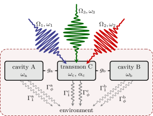
Figure 1: Tripartite system consisting of two superconducting cavities, labeled A and B, coupled via an intermediate (driven) transmon, labeled C. The system interacts with its environment, modeled by individual decay rates for each subsystem.

In the following, we want to engineer a beamsplitter interaction between the two cavities by driving the intermediate transmon appropriately Gao et al. (2018), i.e., we want to engineer a Hamiltonian of the form

$$\mathsf{H}_{\mathrm{BS}}^{\mathrm{AB}}(t)=g_{\mathrm{BS}}(t)\mathsf{a}\mathsf{b}^{\dagger}+g_{\mathrm{BS}}^{*}(t)\mathsf{a}^{\dagger}\mathsf{b}$$ (5)

on the reduced system of the two cavities. Here, $g_{\mathrm{BS}}(t)$ corresponds to the effective interaction strength, i.e., the beamsplitter rate between cavities A and B. One way to realize the interaction is to drive the transmon with two control fields, $\Omega_{1}(t)$ and $\Omega_{2}(t)$, with constant frequencies, $\omega_{1}$ and $\omega_{2}$ Gao et al. (2018). The latter need to fulfill the resonance condition

$$\tilde{\omega}_{\mathrm{b}}-\tilde{\omega}_{\mathrm{a}}=\omega_{2}-\omega_{1},$$ (6)

where $\tilde{\omega}_{\mathrm{a}}$ and $\tilde{\omega}_{\mathrm{b}}$ are the Stark-shifted versions of cavity frequencies $\omega_{\mathrm{a}}$ and $\omega_{\mathrm{b}}$, respectively. The individual Stark shifts are induced by driving the transmon together with its small but finite coupling to each cavity. Note that the Stark shifts are determined primarily by the amplitudes $\Omega_{1}(t)$ and $\Omega_{2}(t)$ of the two control fields and only weakly by their frequencies Zhang et al. (2019). To ensure Eq. (6), the amplitudes should be kept constant — except for a small ramping time $\tau$ at the beginning and end of the protocol, in order to switch the fields on and off smoothly. This can for instance be achieved by choosing

$$\Omega_{k}(t)=\Omega_{k}S(t)$$ (7)

with the shape function

$$S(t)=\begin{cases}\sin^{2}\left(\pi\frac{t}{2\tau}\right),&\qquad t\in[0,\tau),\\ 1,&\qquad t\in[\tau,T-\tau],\\ \sin^{2}\left(\pi\frac{T-t}{2\tau}\right),&\qquad t\in(T-\tau,T],\\ 0,&\qquad\mathrm{else},\end{cases}$$ (8)

where $T$ is the protocol’s total duration.

In the following, we examine whether it is possible to increase the beamsplitter rate, $|g_{\mathrm{BS}}(t)|$, by using an additional control field, respectively more frequencies $\{\omega_{k}\}$, and by exploiting fully time-dependent amplitudes $\{\Omega_{k}(t)\}$. To answer this question, i.e., to tackle this non-trivial control task, we use quantum optimal control theory (OCT) to optimize $\{\omega_{k}\}$ and $\{\Omega_{k}(t)\}$. Briefly, quantum control assumes that a system can be steered by a set of control fields to a desired target. Let $\{\mathcal{E}_{k}(t)\}$ be the set of fields for illustration purposes. OCT provides the tools to derive tailored, i.e., optimized, control fields $\{\mathcal{E}_{k}^{\mathrm{opt}}(t)\}$ realizing the corresponding dynamics, e.g. yielding the smallest error or shortest time Glaser et al. (2015). We will specify the physical aspects of the control problem in Sec. II.2 and the technical details on how to find optimized versions of $\{\omega_{k}\}$ and $\{\Omega_{k}(t)\}$ in Sec. II.3.

II.2 Target operations and encodings

To tackle the control task of realizing a beamsplitter interaction with the extended set of control fields, we must be able to quantify how well the dynamics of the reduced system of the two cavities matches the desired one generated by the “target” Hamiltonian (5). This is technically challenging, since our “figure of interest” is not some accessible and quantifiable feature of the dynamics but rather its generator. An ideal measure would allow for a direct comparison of the target Hamiltonian with the effective Hamiltonian for the reduced system of the two cavities, given the current choice of frequencies $\{\omega_{k}\}$ and amplitudes $\{\Omega_{k}(t)\}$. Unfortunately, it is not possible to derive such an expression for an effective Hamiltonian in case of an arbitrary (yet unknown) choice of $\{\omega_{k}\}$ and $\{\Omega_{k}(t)\}$. However, we can compare the dynamics, which the target and actual Hamiltonian give rise to, by means of comparing various time-evolved states and quantifying their distance with respect to some desired outcome. In detail, we compute the dynamical map $\mathcal{D}_{T,0}^{\mathrm{trgt}}$ that the desired Hamiltonian (5) gives rise to for any initial state $\mathsf{\rho}_{\mathrm{in}}$ and quantify the distance between the desired outcome $\mathsf{\rho}_{\mathrm{trgt}}(T)=\mathcal{D}_{T,0}^{\mathrm{trgt}}[\mathsf{\rho}_{\mathrm{in}}]$ and the actual time-evolved state $\mathsf{\rho}(T)=\mathcal{D}_{T,0}[\mathsf{\rho}_{\mathrm{in}}]$. The dynamical map $\mathcal{D}_{T,0}$ of the actual time-evolution depends on $\{\omega_{k}\}$ and $\{\Omega_{k}(t)\}$. In practice, it is not necessary to evaluate the distance for any $\mathsf{\rho}_{\mathrm{in}}$ but only for a set of basis states spanning the subspace within which we require accurate execution of the protocol. This subspace will be the logical two-qubit subspace in the following. To specify the latter — and thus the set of states for which to evaluate $\mathsf{\rho}(T)=\mathcal{D}_{T,0}[\mathsf{\rho}_{\mathrm{in}}]$ — we first introduce $\{\ket{\overline{n_{\mathrm{a}},n_{\mathrm{b}},n_{\mathrm{c}}}}\}$, the eigenstate basis of the field-free Hamiltonian (II.1). The nomenclature of the eigenstate $\ket{\overline{n_{\mathrm{a}},n_{\mathrm{b}},n_{\mathrm{c}}}}$ is chosen identical to that of the Fock state $\ket{n_{\mathrm{a}},n_{\mathrm{b}},n_{\mathrm{c}}}$ with which it has the largest overlap. Given the eigenstate basis, the target dynamical map $\mathcal{D}_{T,0}^{\mathrm{trgt}}$ yields the time-evolution

$$\mathcal{D}_{T,0}^{\mathrm{trgt}}\left[\ket{\overline{n_{\mathrm{a}},n_{\mathrm{b}},0}}\bra{\overline{n_{\mathrm{a}},n_{\mathrm{b}},0}}\right]=\ket{\overline{n_{\mathrm{b}},n_{\mathrm{a}},0}}\bra{\overline{n_{\mathrm{b}},n_{\mathrm{a}},0}}$$ (9)

for all $n_{\mathrm{a}},n_{\mathrm{b}}=0,1,2,\dots$. In other words, $\mathcal{D}_{T,0}^{\mathrm{trgt}}$ swaps (up to some phase) the states of the two cavities, leaving the transmon invariant.

We seek a $\mathcal{D}_{T,0}$ that yields the same outcome as in Eq. (9) if the frequencies $\{\omega_{k}\}$ and drive amplitudes $\{\Omega_{k}(t)\}$ are chosen appropriately. Let $\mathsf{\rho}_{n_{\mathrm{a}},n_{\mathrm{b}},n_{\mathrm{c}}}=\ket{\overline{n_{\mathrm{a}},n_{\mathrm{b}},n_{\mathrm{c}}}}\bra{\overline{n_{\mathrm{a}},n_{\mathrm{b}},n_{\mathrm{c}}}}$. A measure that becomes zero if and only if $\mathcal{D}_{T,0}$ reproduces the desired outcome of Eq. (9) and is strictly larger otherwise is given by

$$\varepsilon=1-\frac{1}{M^{2}}\sum_{n_{\mathrm{a}},n_{\mathrm{b}}=0}^{M-1}\left\llangle\mathsf{\rho}_{n_{\mathrm{b}},n_{\mathrm{a}},0}\Big{|}\mathcal{D}_{T,0}\left[\mathsf{\rho}_{n_{\mathrm{a}},n_{\mathrm{b}},0}\right]\right\rrangle$$ (10)

with $\left\llangle\mathsf{A}|\mathsf{B}\right\rrangle=\mathrm{tr}\{\mathsf{A}^{\dagger}\mathsf{B}\}$ and $M$ the maximal photon number in the cavities up to which the correct behavior of Eq. (9) is being checked. Note that the perfect beamsplitter interaction of Eq. (5) always gives rise to a perfect swap of the cavity states, i.e., $\varepsilon=0$ holds in case of $\mathcal{D}_{T,0}=\mathcal{D}_{T,0}^{\mathrm{trgt}}$ for arbitrarily large $M$, i.e., arbitrary large photon numbers in the cavities. Furthermore note that we assume the transmon to be initially in its ground state and — since a perfect beamsplitter operation would leave the transmon state unchanged — require $\mathcal{D}_{T,0}$ to return the transmon to its ground state at time $T$.

It is the fact that a perfect beamsplitter interaction always gives rise to a perfect swap of the cavity states that makes it so appealing for continuous variable quantum computing. Any protocol or gate would then work independent of the qubits’ encoding, i.e., independent of the states $\ket{0}_{\mathrm{L}}$ and $\ket{1}_{\mathrm{L}}$ chosen to represent the two logical qubit levels. Instead of evaluating Eq. (10) for large $M$, which requires the propagation of $M^{2}$ initial states, we consider two different encodings and check whether the desired dynamics can be observed in the corresponding logical two-qubit subspace. To this end, we consider an encoding of the logical qubit states in the cavity’s two lowest Fock states, i.e., $\ket{0/1}_{\mathrm{L}}=\ket{0/1}$. The logical two-qubit basis within the tripartite system of the two cavities and the transmon is then given by

$$\ket{0,0,0}_{\mathrm{L}} \equiv\ket{\overline{0,0,0}},$$

$$\ket{0,1,0}_{\mathrm{L}} \equiv\ket{\overline{0,1,0}},$$

$$\ket{1,0,0}_{\mathrm{L}} \equiv\ket{\overline{1,0,0}},$$

$$\ket{1,1,0}_{\mathrm{L}} \equiv\ket{\overline{1,1,0}}.$$ (11)

In contrast to this rather simple encoding, we also consider a binomial encoding Michael et al. (2016) in which case the logical qubit states are given by

$$\ket{0}_{\mathrm{L}}=\frac{\ket{0}+\ket{4}}{\sqrt{2}},\qquad\ket{1}_{\mathrm{L}}=\ket{2}$$ (12)

within each cavity. Thus, the logical two-qubit basis within the tripartite system is given by

$$\ket{0,0,0}_{\mathrm{L}} \equiv\frac{\ket{\overline{0,0,0}}+\ket{\overline{0,4,0}}+\ket{\overline{4,0,0}}+\ket{\overline{4,4,0}}}{2},$$

$$\ket{0,1,0}_{\mathrm{L}} \equiv\frac{\ket{\overline{0,2,0}}+\ket{\overline{4,2,0}}}{\sqrt{2}},$$

$$\ket{1,0,0}_{\mathrm{L}} \equiv\frac{\ket{\overline{2,0,0}}+\ket{\overline{2,4,0}}}{\sqrt{2}},$$

$$\ket{1,1,0}_{\mathrm{L}} \equiv\ket{\overline{2,2,0}}.\vphantom{\frac{1}{\sqrt{2}}}$$ (13)

To compute the error of the protocol, we evaluate

$$\varepsilon=1-\frac{1}{4}\sum_{n_{\mathrm{a}},n_{\mathrm{b}}=0}^{1}\left\llangle\mathsf{\rho}_{n_{\mathrm{b}},n_{\mathrm{a}},0}^{\mathrm{L}}\Big{|}\mathcal{D}_{T,0}\left[\mathsf{\rho}_{n_{\mathrm{a}},n_{\mathrm{b}},0}^{\mathrm{L}}\right]\right\rrangle,$$ (14)

with $\mathsf{\rho}_{n_{\mathrm{a}},n_{\mathrm{b}},n_{\mathrm{c}}}^{\mathrm{L}}=\ket{n_{\mathrm{a}},n_{\mathrm{b}},n_{\mathrm{c}}}_{\mathrm{L}}\bra{n_{\mathrm{a}},n_{\mathrm{b}},n_{\mathrm{c}}}_{\mathrm{L}}$ for the two encodings given in Eqs. (II.2) and (II.2).

II.3 Quantum Optimal Control Theory

We now turn towards OCT, where a control problem is typically converted into the minimization of a cost function. The latter is given by the optimization functional

$$J\left[\left\{\mathcal{E}_{k}\right\},\left\{\mathsf{\rho}_{l}\right\}\right] =\varepsilon\left[\left\{\mathsf{\rho}_{l}(T)\right\}\right]$$ (15)

$$\quad+\int_{0}^{T}\mathrm{d}t\,J_{t}\left[\left\{\mathcal{E}_{k}(t)\right\},\left\{\mathsf{\rho}_{l}(t)\right\},t\right],$$

consisting of the final-time functional $\varepsilon[\{\mathsf{\rho}_{l}(T)\}]$, which quantifies how well the dynamics reaches a desired target at final time $T$, and an intermediate-time functional $J_{t}[\{\mathcal{E}_{k}(t)\},\{\mathsf{\rho}_{l}(t)\},t]$, which captures additional time-dependent costs and constraints. $\left\{\mathsf{\rho}_{l}(t)\right\}$ is a set of time-evolved states where the index $l$ distinguishes different initial states. The choice of $J$ — with $\varepsilon$ its most important part — captures the goal of the control problem. Searching for the control fields that minimize $J$, i.e., solve the control problem, yields optimized fields $\{\mathcal{E}_{k}^{\mathrm{opt}}(t)\}$ that implement the desired dynamics best.

In the following, we use OCT in order to find optimized control fields, i.e., time-dependent drive amplitudes $\{\Omega_{k}^{\mathrm{opt}}(t)\}$, such that they minimize the error $\varepsilon$, Eq. (14). We achieve this in two steps. In a first step, we consider time-independent amplitudes (up to the ramps) as in the original protocol Gao et al. (2018) but we add a third control field with amplitude $\Omega_{3}$ and frequency $\omega_{3}$ to generate the desired dynamics, Eq. (9), in shorter time $T$. In this case, $\varepsilon$ becomes a function of $\Omega_{3}$ and $\omega_{3}$ as well as the final time $T$. We use the gradient-free Nelder-Mead optimization method Nelder and Mead (1965) to search for an optimized set of these three parameters that minimizes $\varepsilon$. In a second step, we then fix the frequencies $\omega_{1},\omega_{2},\omega_{3}$ of the three control fields as well as the final time $T$ and allow their amplitudes, $\Omega_{1}(t),\Omega_{2}(t)$ and $\Omega_{3}(t)$, to be fully time-dependent to minimize $\varepsilon$ even further. We use Krotov’s method for this purpose and briefly summarize its main equations in the following.

Krotov’s method Konnov and Krotov (1999) is an iterative, gradient-based optimization technique with guaranteed monotonic convergence Reich et al. (2012). In order to obtain an update equation for each field $\Omega_{k}(t)$ in Krotov’s method, it is necessary to define $J_{t}$ and formally minimize $J$, cf. Eq. (15). We take Palao and Kosloff (2003)

$$J_{t}\left[\left\{\Omega_{k}(t)\right\}\right]=\sum_{k}\frac{\lambda_{k}}{S(t)}\bigg{[}\Omega_{k}(t)-\Omega_{k}^{\mathrm{ref}}(t)\bigg{]}^{2},$$ (16)

where $\Omega_{k}^{\mathrm{ref}}(t)$ is a reference field for each $\Omega_{k}(t)$, $S(t)$ the shape function from Eq. (8) and $\lambda_{k}$ a numerical parameter that controls the magnitude of update in each iteration. By choosing $\Omega_{k}^{\mathrm{ref}}(t)$ to always be the respective field from the previous iteration, $J_{t}$ will vanish as the optimization converges Palao and Kosloff (2003). Hence, minimizing $J$ becomes identical to minimizing $\varepsilon$, which is the important figure of merit that we seek to minimize in the first place.

With $J_{t}$ from Eq. (16), Krotov’s method yields the update equation Goerz et al. (2014); Reich (2014) 

$$\Omega_{k}^{(i+1)}(t) =\Omega_{k}^{(i)}(t)+\frac{S(t)}{\lambda_{k}}\mathfrak{Re}\left\{\sum_{l}\left\llangle\mathsf{\chi}^{(i)}_{l}(t)\Bigg{|}\frac{\partial\mathcal{L}(t)}{\partial\Omega_{k}}\Big{|}_{\{\Omega^{(i+1)}_{k^{\prime}}(t)\}}\mathsf{\rho}^{(i+1)}_{l}(t)\right\rrangle\right\}.$$ (17)

$\{\mathsf{\rho}^{(i+1)}_{l}(t)\}$ are forward propagated initial states $\{\mathsf{\rho}_{l}(0)\}$, i.e., solutions to the Lindblad master equation

$$\frac{\mathrm{d}}{\mathrm{d}t}\mathsf{\rho}^{(i+1)}_{l}(t)=\mathcal{L}^{(i+1)}(t)\left[\mathsf{\rho}^{(i+1)}_{l}(t)\right]$$ (18)

under the new fields $\{\Omega_{k}^{(i+1)}(t)\}$. $\{\mathsf{\chi}^{(i)}_{l}(t)\}$ are so-called co-states, which are solutions to the adjoint equation of motion

$$\frac{\mathrm{d}}{\mathrm{d}t}\mathsf{\chi}^{(i)}_{l}(t)=\mathcal{L}^{(i)\dagger}(t)\left[\mathsf{\chi}^{(i)}_{l}(t)\right]$$ (19)

under the old fields $\{\Omega_{k}^{(i)}(t)\}$ with boundary condition

$$\mathsf{\chi}^{(i)}_{l}(T)=-\frac{\partial\varepsilon}{\partial\mathsf{\rho}_{l}(T)}\Big{|}_{\{\mathsf{\rho}^{(i)}_{l^{\prime}}(T)\}}.$$ (20)

The initial states $\{\mathsf{\rho}_{l}(0)\}$ are in our case given by the four logical basis states from Eq. (II.2) or Eq. (II.2) depending on which encoding we want to optimize for by minimizing Eq. (14).

We use the QDYN library qdy for solving all equations of motion and for Krotov’s method. The NLopt library Johnson is used for the gradient-free optimizations.

Table 1: Parameters for cavities A and B and transmon C, taken from Ref. Gao et al. (2018).

frequency cavity A	$\omega_{\mathrm{a}}/2\pi$	$5.554\text{\,}\mathrm{GHz}$
frequency cavity B	$\omega_{\mathrm{b}}/2\pi$	$6.543\text{\,}\mathrm{GHz}$
base frequency transmon C	$\omega_{\mathrm{c}}/2\pi$	$5.901\text{\,}\mathrm{GHz}$
anharmonicity transmon C	$\alpha_{\mathrm{c}}/2\pi$	$74\text{\,}\mathrm{MHz}$
coupling between A and C	$g_{\mathrm{a}}/2\pi$	$-19.921\text{\,}\mathrm{MHz}$
coupling between B and C	$g_{\mathrm{b}}/2\pi$	$28.417\text{\,}\mathrm{MHz}$
amplitude driving field 1	$\Omega_{1}/2\pi$	$94.200\text{\,}\mathrm{MHz}$
amplitude driving field 2	$\Omega_{2}/2\pi$	$229.725\text{\,}\mathrm{MHz}$
frequency driving field 1	$\omega_{1}/2\pi$	$6058.000\text{\,}\mathrm{MHz}$
frequency driving field 2	$\omega_{2}/2\pi$	$7049.624\text{\,}\mathrm{MHz}$
ramping time	$\tau$	$50\text{\,}\mathrm{ns}$
relaxation of cavity A	$T_{1}^{\mathrm{a}}$	$1000\text{\,}\mathrm{\SIUnitSymbolMicro s}$
relaxation of cavity B	$T_{1}^{\mathrm{b}}$	$1000\text{\,}\mathrm{\SIUnitSymbolMicro s}$
relaxation of transmon C	$T_{1}^{\mathrm{c}}$	$50\text{\,}\mathrm{\SIUnitSymbolMicro s}$
dephasing of cavity A	$T_{\phi}^{\mathrm{a}}$	$\infty$
dephasing of cavity B	$T_{\phi}^{\mathrm{b}}$	$\infty$
dephasing of transmon C	$T_{\phi}^{\mathrm{c}}$	$50\text{\,}\mathrm{\SIUnitSymbolMicro s}$

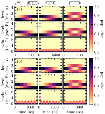
Figure 2: Population dynamics for the three initial states $\ket{\overline{0,1,0}},\ket{\overline{1,0,0}}$ and $\ket{\overline{1,1,0}}$ with $\ket{\overline{0,0,0}}$ omitted as it does not give rise to any cavity excitations. (a) Dynamics under the original two-tone protocol of Ref. Gao et al. (2018) using the parameters from Table 1. (b) Dynamics as in (a) but for a three-tone protocol with optimized but constant amplitude $\Omega_{3}$ and frequency $\omega_{3}$. Note the different time scales. See main text for details. The term ”levels” refers to the bare Fock states $\ket{n_{\mathrm{a}}}$ and $\ket{n_{\mathrm{b}}}$ in case of cavities A and B and to the anharmonic ladder states $\ket{n_{\mathrm{c}}}$ of the bare transmon in case of transmon C.

III Engineering Strong Beamsplitter Interaction via Sideband Transitions

In this section, we demonstrate how to use OCT in order to engineer a beamsplitter interaction between cavities A and B that is stronger than the one presented in Ref. Gao et al. (2018).

III.1 Two-tone vs. three-tone protocol

We take the physical parameters as reported in Ref. Gao et al. (2018), cf. Table 1, and start by analyzing the original two-tone protocol. The two tones’ amplitudes, $\Omega_{1}$ and $\Omega_{2}$, and frequencies, $\omega_{1}$ and $\omega_{2}$, are chosen to satisfy the resonance condition (6) and therefore give rise to the desired beamsplitter interaction, cf. Eq. (5). If we assume Fock encoding in Eq. (14), the subspace for which to test the protocol is defined by the four initial states $\ket{\overline{0,0,0}},\ket{\overline{0,1,0}},\ket{\overline{1,0,0}}$ and $\ket{\overline{1,1,0}}$. Figure 2(a) shows the population dynamics for these initial states under the original two-tone protocol Gao et al. (2018). As expected, the dynamics swaps the initial states of cavity A and B for $\ket{\overline{0,1,0}}$ and $\ket{\overline{1,0,0}}$ and leaves the states $\ket{\overline{0,0,0}}$ and $\ket{\overline{1,1,0}}$ invariant at final time $T=$6780\text{\,}\mathrm{ns}$$. This invariance does not hold at intermediate times, cf. the dynamics of $\ket{\overline{1,1,0}}$. Note that the transmon is only weakly excited (its time-averaged ground state population is 0.73, cf. Eq. (39)), which is in agreement with the theory of the two-tone protocol Zhang et al. (2019).The two tones are switched on and off smoothly by a ramp $S(t)$. This transfers the transmon smoothly from its ground state into an energetically low-lying Floquet state at intermediate times and back to the ground state at final time. This is the reason for the small but non-vanishing population in some lower bare transmon levels seen in Fig. 2(a).

We now add a third control field with amplitude $\Omega_{3}$ and frequency $\omega_{3}$ with the purpose to realize the desired swap, cf. Eq. (9), in a shorter total time $T$. As outlined in Sec. II.3, we use a gradient-free optimization to find optimized values for the three parameters, i.e., $\Omega_{3},\omega_{3},T$. We kept the parameters of the other two control fields, $\Omega_{1},\Omega_{2},\omega_{1},\omega_{2}$, fixed to limit the number of optimization parameters and thus ease the optimization procedure. We find the optimized parameters for the third drive to be

$$\Omega_{3}/2\pi=$271.093\text{\,}\mathrm{MHz}$,\qquad\omega_{3}/2\pi=$6.749\text{\,}\mathrm{GHz}$$$ (21)

and the protocol duration $T=$1492\text{\,}\mathrm{ns}$$, which is about five times shorter than $T=$6780\text{\,}\mathrm{ns}$$ in case of the two-tone protocol. Figure 2(b) shows the corresponding population dynamics for the three-tone protocol. In comparison with the dynamics of the original two-tone protocol, cf. Fig. 2(a), the dynamics of the three-tone protocol looks very similar but is approximately five times faster. We find the coherent errors to be $\varepsilon_{2}=0.5\%$ for the two-tone protocol and $\varepsilon_{3}=2.6\%$ for the three-tone protocol. When decoherence is taken into account, the errors increase to $\varepsilon_{2}=8.6\%$ and $\varepsilon_{3}=5.0\%$ for the two-tone and three-tone protocol, respectively. As expected, the increase in error is much smaller for the significantly faster three-tone protocol compared to the original two-tone protocol and compensates the previously larger coherent error of the three-tone protocol. We will analyze the impact of decoherence in more detail in Sec. IV.

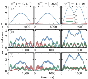
Figure 3: Mutual information $\mathcal{I}$ between all pairs of subsystems A, B and C. Panels (a) and (b) correspond to the two- and three-tone protocol and the population dynamics shown in Fig. 2(a) and (b), respectively. Panel (c) corresponds to the three-tone protocol that has been further fine-tuned by a gradient-based optimization technique (see main text for details).

In order to understand the similarities and differences of the two- and three-tone protocols, we inspect the correlations between any two of the three subsystems of cavities A and B and transmon C as a function of time. Figure 3(a) and (b) show the mutual information $\mathcal{I}$, as a measure for the correlations between two subsystems Henderson and Vedral (2001), for the two- and three-tone protocol, respectively. The mutual information between two subsystems, say cavities A and B, is defined as

$$\mathcal{I}_{\mathrm{ab}}=\mathcal{P}(\mathsf{\rho}_{\mathrm{a}})+\mathcal{P}(\mathsf{\rho}_{\mathrm{b}})-\mathcal{P}(\mathsf{\rho}_{\mathrm{ab}}),$$ (22)

with $\mathcal{P}(\mathsf{\rho}_{\mathrm{x}})=-\mathrm{tr}\{\mathsf{\rho}_{\mathrm{x}}\ln(\mathsf{\rho}_{\mathrm{x}})\}$ the von Neumann entropy of state $\mathsf{\rho}_{\mathrm{x}}$ and $\mathsf{\rho}_{\mathrm{ab}}=\mathrm{tr}_{\mathrm{c}}\{\mathsf{\rho}\}$, $\mathsf{\rho}_{\mathrm{a}}=\mathrm{tr}_{\mathrm{b}}\{\mathsf{\rho}_{\mathrm{ab}}\}$ and $\mathsf{\rho}_{\mathrm{b}}=\mathrm{tr}_{\mathrm{a}}\{\mathsf{\rho}_{\mathrm{ab}}\}$ the reduced states of subsystems AB, A and B, respectively, calculated from the state $\mathsf{\rho}=\mathsf{\rho}(t)$ of the full tripartite system. As can be seen for the two-tone protocol, cf. Fig. 3(a), only the two cavities build up correlations over time, whereas the transmon C stays uncorrelated with both at all times. At final time $T$, both cavities are again uncorrelated. This behavior changes for the three-tone protocol, cf. Fig. 3(b), as it gives rise to additional intermediate correlations between both cavities and the transmon as well as remaining, non-vanishing correlations at final time $T$. Closer inspection of the dynamics for the initial state $\ket{\overline{1,0,0}}$ ($\ket{\overline{0,1,0}}$) reveals that, in the first half of the protocol, cavity A (B) primarily correlates with the transmon while in the second half primarily cavity B (A) correlates with the transmon. In particular correlations that are built up in the second half do not vanish at final time $T$. This is a reason for the larger coherent error $\varepsilon_{3}$ of the three-tone protocol. We show in Appendix A that, despite the emerging correlations between cavities and transmon, the three-tone protocol still engineers the intended beamsplitter interaction (5).

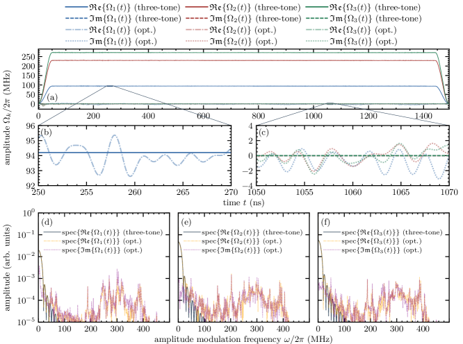
Figure 4: Panel (a) shows the time-dependent amplitudes $\Omega_{k}(t)$ of the three-tone protocol (solid and dashed lines) and their fine-tuned versions (dashed-dotted and dotted lines), while (b) and (c) show a close-up view. The coherent errors for the three-tone protocol and its fine-tuned version are $\varepsilon_{3}=2.6\%$ and $\varepsilon_{3,\mathrm{grad}}=0.2\%$, respectively. Panels (d)-(f) show the spectra (the absolute value of the Fourier transform) of $\mathfrak{Re}\{\Omega_{k}(t)\}$ and $\mathfrak{Im}\{\Omega_{k}(t)\}$ for the three-tone protocol (solid lines) and its fine-tuned version (dashed-dotted and dotted lines), respectively. Note that $\mathfrak{Im}\{\Omega_{k}(t)\}$ is zero for the three-tone protocol and hence its spectrum is omitted. The dashed-dotted and dotted lines are heavily overlapping and are thus hard to distinguish visually. The base-frequencies for the three tones are given in Table 1 and Eq. (21).

III.2 Fine-tuned three-tone protocol

A possibility to reduce the coherent error $\varepsilon_{3}$ of the three-tone protocol is to fine-tune it further with gradient-based optimization, as outlined in Sec. II.3, using the constant values of the three-tone protocol (up to ramping times) as guess fields. While each field $\Omega_{k}(t)$ has its base frequency $\omega_{k}$, cf. Eq. (II.1), allowing for fully time-dependent and complex $\Omega_{k}(t)$ introduces new frequencies, i.e., the protocol is strictly speaking no longer a three-tone protocol. In order to prevent the bandwidth of the amplitude modulations to become too large and experimentally unfeasible, we truncate the spectrum of $\mathfrak{Re}\{\Omega_{k}(t)\}$ and $\mathfrak{Im}\{\Omega_{k}(t)\}$ after each iteration of the optimization by multiplying the spectrum with the spectral shape function

$$S_{\mathrm{bw}}(\omega)=\begin{cases}1,&\qquad|\omega|\in[0,\omega_{\mathrm{co}}-\Delta\omega_{\mathrm{co}}]\\ \sin^{2}\left(\pi\frac{|\omega|-\omega_{\mathrm{co}}}{2\Delta\omega_{\mathrm{co}}}\right),&\qquad|\omega|\in(\omega_{\mathrm{co}}-\Delta\omega_{\mathrm{co}},\omega_{\mathrm{co}}],\\ 0,&\qquad\mathrm{else},\end{cases}$$ (23)

where $\omega_{\mathrm{co}}$ is a cutoff frequency. Here, $\Delta\omega_{\mathrm{co}}$ is necessary to truncate the spectra smoothly and guarantee a smooth shape of $\Omega_{k}(t)$ in time domain.

Figure 4(a)-(c) compares the real and imaginary parts of $\Omega_{k}(t)$ for the three-tone protocol with the further fine-tuned version. As can be seen, the gradient-based optimization adapts the amplitudes slightly by adding minor oscillations. Despite these apparently small differences, the coherent protocol error reduces from $\varepsilon_{3}=2.6\%$ to $\varepsilon_{3,\mathrm{grad}}=0.2\%$. The spectra of $\mathfrak{Re}\{\Omega_{k}(t)\}$ and $\mathfrak{Im}\{\Omega_{k}(t)\}$ of the three-tone protocol and its further fine-tuned version are shown in Fig. 4(d)-(f). The three-tone protocol has a single dominant peak at modulation frequency $\omega=0$ with only minor non-zero elements due to the ramping. After optimization, new amplitude modulation frequencies up to $\omega/2\pi\sim$400\text{\,}\mathrm{MHz}$$ appear, reflecting our choice of $\omega_{\mathrm{co}}/2\pi=$500\text{\,}\mathrm{MHz}$$ and $\Delta\omega_{\mathrm{co}}/2\pi=$100\text{\,}\mathrm{MHz}$$ for truncating the spectra. Compared to the spectral amplitude of the central peak at $\omega=0$, these new frequencies have spectral amplitudes that are at least two orders of magnitude smaller. This is consistent with the amplitudes $\Omega_{k}(t)$ remaining almost constant in time with only small oscillations on top, cf. Fig. 4(b) and (c). The effect of the modulations can be seen in Fig. 3(c), which shows the mutual information between the three subsystems. While the overall structure of the correlation dynamics is preserved compared to the three-tone protocol in Fig. 3(b), the fine-tuned amplitudes $\Omega_{k}(t)$ erase all correlations at final time $T$. This concerns especially those correlations between cavity A/B and the transmon C built up when starting in states $\ket{\overline{0,1,0}}$ or $\ket{\overline{1,0,0}}$ which do not vanish at final time $T$ under the non-fine-tuned three-tone protocol. Despite the difference in the correlation dynamics and final errors, the population dynamics for the fine-tuned protocol is visually almost identical to the three-tone protocol shown in Fig. 2(b) (data not shown).

Note that technically, it would also be possible to carry out the optimization with a single field instead of optimizing the three tones individually. Motivated by Eq. (II.1), one could for instance define the effective field $\mathcal{E}_{\mathrm{eff}}(t)=\sum_{k}\Omega_{k}(t)e^{-\textup{i}\delta_{k}t}$ and optimize its real and imaginary part. This carries the same information. However, an optimization with three individual tones allows for more flexibility when controlling each field’s update, e.g. by truncating the spectra (as used above) or by choosing which tones should be updated at all.

It is of course possible to apply the gradient-based optimization — including restricting the amplitude modulation frequencies by spectral truncation — also to the two-tone protocol directly. This lowers the coherent error from $\varepsilon_{2}=0.5\%$ to $\varepsilon_{2,\mathrm{grad}}<0.1\%$. The changes to the amplitudes $\Omega_{k}(t)$ are even smaller than the ones shown in Fig. 4 for the three-tone protocol. However, for both the two- and three-tone protocol, decoherence is the dominant source of error which increases to $\varepsilon_{2,\mathrm{grad}}=9.2\%$ and $\varepsilon_{3,\mathrm{grad}}=3.2\%$, respectively, once decoherence is taken into account.

A subtle but important fact can be noticed when comparing the change between the coherent protocol errors under the fine-tuned protocols, once decoherence is accounted for. In detail, the increase due to decoherence is slightly larger for the fine-tuned versions of the two- and three-tone protocols compared to their non-fine-tuned versions despite unchanged duration $T$. This is due to the fact that — for reasons to keep the numerical costs manageable — the optimization itself is carried out entirely in Hilbert space, i.e., without taking decoherence into account explicitly. Instead, we account for it implicitly by penalizing control solutions that involve excitation of higher transmon levels which suffer more from decoherence. Although the dynamics under the fine-tuned protocols does not utilize higher transmon excitations, it exploits coherences between energetically low-lying but populated levels — especially those between the transmon’s bare ground and first excited state. Hence, any deviation from the desired dynamics of the coherences due to decoherence causes the protocol error to increase. In case of the two-tone protocol, the increase for the fine-tuned version is larger than that of the original version, illustrating the fine-tuned protocol’s somewhat increased sensitivity to decoherence.

Table 2: Protocol errors for the original two-tone protocol, $\varepsilon_{2}$, the three-tone protocol, $\varepsilon_{3}$, and their respective fine-tuned versions, $\varepsilon_{2,\mathrm{grad}}$ and $\varepsilon_{3,\mathrm{grad}}$. The errors are given for both Fock and binomial encoding, cf. Eq. (14). Decoherence times are as in Table 1.

	coherent	error including	encoding
	error	decoherence
$\varepsilon_{2}$	$0.5\%$	$8.6\%$	Fock
$\varepsilon_{2,\mathrm{grad}}$	$<0.1\%$	$9.2\%$	Fock
$\varepsilon_{3}$	$2.6\%$	$5.0\%$	Fock
$\varepsilon_{3,\mathrm{grad}}$	$0.2\%$	$3.2\%$	Fock
$\varepsilon^{\mathrm{binom}}_{2}$	$43.9\%$	$53.9\%$	binomial
$\varepsilon^{\mathrm{binom}}_{2,\mathrm{grad}}$	$0.8\%$	$35.3\%$	binomial
$\varepsilon^{\mathrm{binom}}_{3}$	$58.7\%$	$60.6\%$	binomial
$\varepsilon^{\mathrm{binom}}_{3,\mathrm{grad}}$	$2.0\%$	$11.0\%$	binomial

So far we have discussed whether the engineered dynamics behaves as intended when the qubit is encoded in the two lowest Fock states of each cavity. However, as emphasized earlier, it would be advantageous to have a protocol that works in a codeword-agnostic way. Thus, as an alternative to the qubit being encoded in the two lowest Fock states, we also employ a binomial encoding Michael et al. (2016). In this case, the error — in the following called $\varepsilon^{\mathrm{binom}}$ — is still given by Eq. (14) but the latter is evaluated for the logical basis states of Eq. (II.2). We find coherent errors $\varepsilon^{\mathrm{binom}}_{2}=43.9\%$ and $\varepsilon^{\mathrm{binom}}_{3}=58.7\%$ for the two-tone protocol of Ref. Gao et al. (2018) and the three-tone protocol, respectively. Taking these protocols again as starting point for a gradient-based optimization — here without frequency truncation — we find coherent errors of $\varepsilon^{\mathrm{binom}}_{2,\mathrm{grad}}=0.8\%$ and $\varepsilon^{\mathrm{binom}}_{3,\mathrm{grad}}=2.0\%$, respectively . While the two- and three-tone protocol do not act as codeword-agnostic as desired, our results indicate that it is possible to adapt each protocol for a given encoding using OCT. Note that these errors are obtained without taking decoherence in account. With decoherence, they become $\varepsilon^{\mathrm{binom}}_{2}=53.9\%$ and $\varepsilon^{\mathrm{binom}}_{3}=60.6\%$ for the two- and three-tone protocol, respectively, and $\varepsilon^{\mathrm{binom}}_{2,\mathrm{grad}}=35.3\%$ and $\varepsilon^{\mathrm{binom}}_{3,\mathrm{grad}}=11.0\%$ for the fine-tuned versions. A summary of all errors, with and without decoherence, is provided in Table 2.

III.3 Analysis of the beamsplitter interaction in the three-tone protocol

We now seek to understand why a third tone gives rise to significantly faster swaps, respectively stronger beamsplitter interaction. To this end, we first notice that the gradient-free optimization chooses the third frequency $\omega_{3}$, cf. Eq. (21), such as to give rise to near-resonant sideband couplings between cavity A/B and transmon C. The sideband couplings are induced by the beating between the third drive and the first two drives. While satisfying Eq. (6) activates the beamsplitter interaction in the original two-tone protocol, we can define a similar resonance condition that needs to be fulfilled for activating the cavity-transmon sideband couplings. It reads

$$\tilde{\omega}_{\mathrm{a}}-\tilde{\omega}_{\mathrm{c}} =\omega_{3}-\omega_{2}+\Delta_{\mathrm{a}},$$

$$\tilde{\omega}_{\mathrm{b}}-\tilde{\omega}_{\mathrm{c}} =\omega_{3}-\omega_{1}+\Delta_{\mathrm{b}},$$ (24)

where $\tilde{\omega}_{\mathrm{c}}$ is the Stark-shifted version of $\omega_{\mathrm{c}}$ and $\Delta_{\mathrm{a}}$ and $\Delta_{\mathrm{b}}$ are detunings from the corresponding perfect sideband couplings between cavity A/B and transmon C, respectively. In order to fulfill the beamsplitter resonance condition (6), we need $\Delta_{\mathrm{a}}\approx\Delta_{\mathrm{b}}$. We thus set $\Delta_{\mathrm{a}}=\Delta_{\mathrm{b}}=\Delta$.

In the following, we use a similar approach as in Ref. Zhang et al. (2019), where the effective beamsplitter Hamiltonian (5) was derived analytically from the tripartite system, including the transmon. The derivation just assumed a two-tone protocol with both frequencies fulfilling the resonance condition (6). Here, we modify the approach of Ref. Zhang et al. (2019) to include the sideband couplings. We also seek to derive an effective Hamiltonian that describes the effective interaction of the two cavities. In contrast to the two-tone protocol, our derivation needs to capture both the cavity-cavity beamsplitter interaction, generated by fulfilling the resonance condition (6), as well as the cavity-transmon sideband coupling, generated by fulfilling Eq. (III.3) near-resonantly, i.e., with a small, but non-zero $\Delta$. Our derivation can thus be seen as an extension of the derivation done in Ref. Zhang et al. (2019). Ultimately, we will compare SWAP times predicted analytically by our derivation (carried out in the following) and semi-analytically using a method from Ref. Zhang et al. (2019) with numerically obtained ones.

First, we assume a weak transmon anharmonicity $\alpha_{\mathrm{c}}\ll|\omega_{\mathrm{a},\mathrm{b}}-\omega_{\mathrm{c}}|$ and diagonalize the quadratic and field-free part of Hamiltonian (II.1) to obtain the eigenmodes. The associated lowering operators for the eigenmodes are $\mathsf{A},\mathsf{B}$ and $\mathsf{C}$. For weak transmon-cavity couplings, one can identify $\mathsf{A}$ and $\mathsf{B}$ as the “cavity-like” eigenmodes that have the largest overlap with the bare cavity modes $\mathsf{a}$ and $\mathsf{b}$ and $\mathsf{C}$ is a “transmon-like” eigenmode. Next, we express the bare transmon operator $\mathsf{c}$ as a function of the eigenmodes of the quadratic, field-free Hamiltonian. In addition to the coupling-induced mode mixing of the bare transmon modes, we also want to capture the effect of the drives and express it in the eigenmode representation of $\mathsf{c}$. To this end, we exploit that for weakly anharmonic transmons the major effect of the drives is to induce a linear displacement of the transmon mode. Combining the coupling-induced mode mixing and the drive-induced displacement of the mode, we find

$$\mathsf{c}\rightarrow\xi_{\mathrm{a}}\mathsf{A}+\xi_{\mathrm{b}}\mathsf{B}+\xi_{\mathrm{c}}\mathsf{C}+\sum_{k=1}^{3}\xi_{k}e^{-\textup{i}\omega_{k}t},$$ (25)

where $\xi_{\mathrm{a}(\mathrm{b})}\approx g_{\mathrm{a}(\mathrm{b})}/\delta_{\mathrm{a}(\mathrm{b})}$, $\xi_{\mathrm{c}}\approx 1$, and $\xi_{k}=\Omega_{k}/\delta_{k}$ for $k=1,2,3$. By substituting Eq. (25) into Hamiltonian (II.1) and transforming into a rotating frame — similar to that from Hamiltonian (II.1) to Hamiltonian (II.1) — we arrive at

$$\mathsf{H}_{\mathrm{eff},1}(t) =g_{\mathrm{AB}}\mathsf{A}^{\dagger}\mathsf{B}+g_{\mathrm{AB}}^{*}\mathsf{A}\mathsf{B}^{\dagger}$$

$$\quad+g_{\mathrm{a}}^{\mathrm{sb}}e^{\textup{i}\Delta t}\mathsf{A}^{\dagger}\mathsf{\sigma}_{-}+g_{\mathrm{a}}^{\mathrm{sb}*}e^{-\textup{i}\Delta t}\mathsf{A}\mathsf{\sigma}_{+}$$

$$\quad+g_{\mathrm{b}}^{\mathrm{sb}}e^{\textup{i}\Delta t}\mathsf{B}^{\dagger}\mathsf{\sigma}_{-}+g_{\mathrm{b}}^{\mathrm{sb}*}e^{-\textup{i}\Delta t}\mathsf{B}\mathsf{\sigma}_{+},$$ (26)

where we have only kept resonant and near-resonant terms. We also truncate the transmon Hilbert space to two levels, replacing $\mathsf{C}$ and $\mathsf{C}^{\dagger}$ by $\mathsf{\sigma}_{-}$ and $\mathsf{\sigma}_{+}$. The cavity-cavity coupling $g_{\mathrm{AB}}$ and transmon-cavity sideband couplings $g_{\mathrm{a}}^{\mathrm{sb}}$ and $g_{\mathrm{b}}^{\mathrm{sb}}$ are given by

$$g_{\mathrm{AB}} =-2\alpha_{\mathrm{c}}\xi_{1}\xi_{2}^{*}\xi_{\mathrm{a}}^{*}\xi_{\mathrm{b}},$$

$$g_{\mathrm{a}}^{\mathrm{sb}} =-2\alpha_{\mathrm{c}}\xi_{2}^{*}\xi_{3}\xi_{\mathrm{a}}^{*}\xi_{\mathrm{c}},$$

$$g_{\mathrm{b}}^{\mathrm{sb}} =-2\alpha_{\mathrm{c}}\xi_{1}^{*}\xi_{3}\xi_{\mathrm{b}}^{*}\xi_{\mathrm{c}}.$$ (27)

In a further transformation, we move into a rotating frame with respect to $\Delta$ where Eq. (III.3) becomes time-independent,

$$\mathsf{H}_{\mathrm{eff},2} =\frac{\Delta}{2}\mathsf{\sigma}_{\mathrm{z}}+g_{\mathrm{AB}}\mathsf{A}^{\dagger}\mathsf{B}+g_{\mathrm{AB}}^{*}\mathsf{A}\mathsf{B}^{\dagger}$$

$$\quad+g_{\mathrm{a}}^{\mathrm{sb}}\mathsf{A}^{\dagger}\mathsf{\sigma}_{-}+g_{\mathrm{a}}^{\mathrm{sb}*}\mathsf{A}\mathsf{\sigma}_{+}$$

$$\quad+g_{\mathrm{b}}^{\mathrm{sb}}\mathsf{B}^{\dagger}\mathsf{\sigma}_{-}+g_{\mathrm{b}}^{\mathrm{sb}*}\mathsf{B}\mathsf{\sigma}_{+}.$$ (28)

This Hamiltonian describes the dynamics of two degenerate modes coupled to each other and to a detuned two-level system. In the limit when $|g_{\mathrm{a}}^{\mathrm{sb}}|,|g_{\mathrm{b}}^{\mathrm{sb}}|\ll|\Delta|$ holds, Eq. (III.3) can be diagonalized perturbatively in $|g_{\mathrm{a},\mathrm{b}}^{\mathrm{sb}}/\Delta|$. To second order, we obtain

$$\mathsf{H}_{\mathrm{eff},3}=\mathsf{g}_{\mathrm{BS}}\mathsf{A}^{\dagger}\mathsf{B}+\mathsf{g}_{\mathrm{BS}}^{*}\mathsf{A}\mathsf{B}^{\dagger}$$ (29a)

with

$$\mathsf{g}_{\mathrm{BS}}=g_{\mathrm{AB}}\mathsf{\mathbbm{1}}-\frac{g_{\mathrm{a}}^{\mathrm{sb}}g_{\mathrm{b}}^{\mathrm{sb}*}}{\Delta}\mathsf{\sigma}_{\mathrm{z}}.$$ (29b)

Note that we neglect terms $\sim\mathsf{A}^{\dagger}\mathsf{A}$ and $\sim\mathsf{B}^{\dagger}\mathsf{B}$ since they represent shifts of the cavity eigenmodes and can be simply compensated by adapting the drive frequencies. Equation (29a) resembles the desired beamsplitter interaction, cf. Eq. (5), but has a slightly more complex structure of the operator $\mathsf{g}_{\mathrm{BS}}$. It contains the “standard” beamsplitter interaction — here given by the term scaling with $g_{\mathrm{AB}}$ — that originates from having two drives which fulfill the resonance condition (6) and additionally the sideband-induced couplings between cavities and transmon. The latter originate from the third drive and effectively amplify the beamsplitter interaction. This gives rise to the faster SWAP operation as observed in Fig. 2.

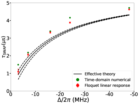
Figure 5: Comparison of the protocol times as obtained numerically (green dots) and from analytical calculations including one from Floquet theory in the spirit of Ref. Zhang et al. (2019) (red dots) and one using the effective theory from Eqs. (29a) and (29b) (black solid line). Note that approximated versions of $\Delta$ and other Stark-shifted parameters have been used here as the exact Stark shifts are not known analytically. This is reflected by the error bars for the Floquet theory and the black dashed lines for the effective theory. The lower (upper) error bars are obtained using a value of $\Delta/2\pi$ that is $-(+)$1\text{\,}\mathrm{MHz}$$ away from the value indicated on the horizontal axis.

Table 3: Further three-tone protocols, obtained via gradient-free optimization, with all other parameters as given in Table. 1 and $\Omega_{3}$ as in Eq. (21).

$\omega_{2}/2\pi$ (MHz)	$\omega_{3}/2\pi$ (MHz)	$T$ (ns)	$\varepsilon_{3}$
7049.654	6752.475	2180.4	$0.8\%$
7049.673	6761.585	3391.8	$0.7\%$
7049.699	6770.048	4158.8	$1.9\%$
7049.665	6793.903	4715.0	$0.7\%$

In order to analyze how well the effective theory of Eqs. (29a) and (29b) describes the three-tone protocol shown in Fig. 2(b), we calculate $\mathsf{g}_{\mathrm{BS}}$ for the parameters in Table 1 and the third drive in Eq. (21). We find $g_{\mathrm{AB}}/2\pi=-$0.045\text{\,}\mathrm{MHz}$$, $g_{\mathrm{a}}^{\mathrm{sb}}/2\pi=-$0.54\text{\,}\mathrm{MHz}$$, $g_{\mathrm{b}}^{\mathrm{sb}}/2\pi=-$1.26\text{\,}\mathrm{MHz}$$ and $\Delta/2\pi\approx-$3\text{\,}\mathrm{MHz}$$. This gives rise to an effective beamsplitter interaction of $g_{\mathrm{BS}}/2\pi=-$0.27\text{\,}\mathrm{MHz}$$  and thus to a SWAP time of $T\approx$924\text{\,}\mathrm{ns}$$. We conjecture that the discrepancy of the analytically predicted SWAP time with respect to the numerically observed one of $T=$1492\text{\,}\mathrm{ns}$$ is caused by $|g_{\mathrm{a}}^{\mathrm{sb}}|,|g_{\mathrm{b}}^{\mathrm{sb}}|\ll|\Delta|$ — which needs to hold for an accurate analytical predictions — not being fulfilled sufficiently well.

To verify this conjecture in more detail, we evaluate Eq. (29b) — and the SWAP time it gives rise to — for further three-tone protocols, where the respective choice of the third frequency $\omega_{3}$ gives rise to larger $|\Delta|$ such that $|g_{\mathrm{a}}^{\mathrm{sb}}|,|g_{\mathrm{b}}^{\mathrm{sb}}|\ll|\Delta|$ is better satisfied. This also allows to investigate the impact of $|\Delta|$ on emerging cavity-transmon correlations and the protocol error, which is not evident from the analytical treatment so far. Possible sets of parameters for three-tone protocols can easily be found using gradient-free optimization as described in Sec. II.3. In these optimizations, we only allow $\omega_{2}$ and $\omega_{3}$ to change in addition to $T$ and keep all three amplitudes as well as $\omega_{1}$ fixed by their values in Table 1 and Eq. (21). The reason behind this choice is that $\omega_{3}$ primarily defines $\Delta$ while adapting $\omega_{2}$ is required to correct for potential Stark shifts in Eq. (6). The latter was assumed to hold while deriving Eqs. (29a) and (29b). Table 3 presents a few optimization results. We now use Eq. (29b) to calculate $g_{\mathrm{BS}}$ and its corresponding SWAP time for each set of parameters. In Fig. 5 we compare the calculated SWAP times (black, solid line) with those obtained numerically (green dots), cf. Table 3, and with the predictions of the semi-analytical method (red dots) developed in Ref. Zhang et al. (2019). In the latter, the drives are treated non-perturbatively using Floquet theory and the cavity-transmon couplings are treated perturbatively using linear response theory. Appendix B summarizes the details of this method. We observe a qualitative agreement between the methods and attribute the small remaining discrepancies to the approximations made within each method. Figure 5 suggests that Eqs. (29a) and (29b) indeed provide the correct physical intuition for the speed-up of the three-tone protocol compared to the original two-tone protocol. In other words, the speed-up is due to exploiting sideband couplings between the cavities and the transmon.

This explanation is also in agreement with the correlations emerging between cavities and transmon under the three-tone protocol, cf. Fig. 3(b), as these correlations are not present under the original two-tone protocol, cf. Fig. 3(a). We observe a clear correspondence between the quantity $\Delta$, cf. Eq. (29b), and the emergence of cavity-transmon correlations. By comparing the correlation dynamics for all parameter sets of Table 3 (data not shown), we see a smooth transition from behavior as in Fig. 3(b) for the fastest three-tone protocol with smallest $|\Delta|$, to behavior as in Fig. 3(a) for the slowest three-tone protocol with largest $|\Delta|$. This is also evident when inspecting the coherent errors $\varepsilon_{3}$ of the three-tone protocols in Table 3. Almost all sets of parameters give rise to coherent protocol errors $\varepsilon_{3}<1\%$ and are thus smaller than the coherent error $\varepsilon_{3}=2.6\%$ for three-tone protocol presented in Fig. 3(b). We see this as evidence that the cavity-transmon correlations are mainly responsible for the coherent error $\varepsilon_{3}$ in the three-tone protocol and ultimately prevent to find even faster protocol.

We conclude that, on one hand, small $|\Delta|$ is in general advantageous for fast three-tone protocols, i.e., for $|g_{\mathrm{BS}}|$ to be large, cf. Eq. (29b). On the other hand, $|\Delta|$ should not be chosen too small such as to keep the coherent error due to non-vanishing correlations between cavities and transmon at final time $T$ at bay. From a coherent perspective, slower protocols are thus favorable. However, once decoherence is taken into account, protocols should typically be as fast as possible. The optimal protocol balances coherent error and the additional error from decoherence.

Finally, it should be mentioned that the calculations employing Floquet and linear response theory — used to determine the red dots in Fig. 5 and detailed in Appendix B — also provide an understanding of the emerging Kerr non-linearities caused by the third drive. These non-linearities seem to increase significantly (data not shown) compared to those induced by the original two-tone protocol Gao et al. (2018). Since the detrimental impact of such cavity non-linearities for the SWAP operations becomes larger for higher photonic states of the cavities, this might provide an explanation for the observed large coherent protocol errors in case of qubit encodings involving higher photon numbers. For a detailed study of drive-induced non-linearities of cavity modes see Ref. Zhang et al. (2021).

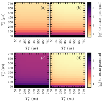
Figure 6: Influence of decoherence on the error $\varepsilon_{2}$ of the original two-tone protocol (a) as well as its fine-tuned version (b) and the error $\varepsilon_{3}$ of the three-tone protocol (c) as well as its fine-tuned version (d). Note that the relaxation times, $T_{1}^{\mathrm{a}}$ and $T_{1}^{\mathrm{b}}$, and pure dephasing times, $T_{\phi}^{\mathrm{a}}$ and $T_{\phi}^{\mathrm{b}}$, for both cavities are fixed in all panels to those values given in Table 1 and only the times for the transmon are varied.

IV Prospects for High-Fidelity Protocols in the Presence of Noise

We now study how the protocols will perform once the coherence times of transmons become better. So far we have assumed the transmon relaxation and pure dephasing times to be $T_{1}^{\mathrm{c}}=$50\text{\,}\mathrm{\SIUnitSymbolMicro s}$$ and $T_{\phi}^{\mathrm{c}}=$50\text{\,}\mathrm{\SIUnitSymbolMicro s}$$. However, better devices exist already with recently reported relaxation times up to $T_{1}^{\mathrm{c}}=$500\text{\,}\mathrm{\SIUnitSymbolMicro s}$$ Wang et al. (2022) and dephasing times up to $T_{\phi}^{\mathrm{c}}=$300\text{\,}\mathrm{\SIUnitSymbolMicro s}$$ Place et al. (2021). In order to investigate how the protocol errors change for better transmon devices, we gradually increase both $T_{1}^{\mathrm{c}}$ and $T_{\phi}^{\mathrm{c}}$ from $50\text{\,}\mathrm{\SIUnitSymbolMicro s}$ to $750\text{\,}\mathrm{\SIUnitSymbolMicro s}$. While the latter times might still be out of reach for current devices, we consider them here to give some perspective for possible future improvement. Figure 6(a) and (b) show how the errors $\varepsilon_{2}$ and $\varepsilon_{2,\mathrm{grad}}$ of the original two-tone protocol and its fine-tuned version improve when $T_{1}^{\mathrm{c}}$ and $T_{\phi}^{\mathrm{c}}$ increase. As can be seen, both errors show a weak dependence on $T_{1}^{\mathrm{c}}$ (on the order of $\sim 0.1\%$) while they rapidly decrease when increasing $T_{\phi}^{\mathrm{c}}$. For the recently reported values of $T_{1}^{\mathrm{c}}=$500\text{\,}\mathrm{\SIUnitSymbolMicro s}$$ and $T_{\phi}^{\mathrm{c}}=$300\text{\,}\mathrm{\SIUnitSymbolMicro s}$$, we find $\varepsilon_{2}=2.5\%$ and $\varepsilon_{2,\mathrm{grad}}=2.2\%$, which is further lowered to $\varepsilon_{2}=1.8\%$ and $\varepsilon_{2,\mathrm{grad}}=1.3\%$ for $T_{1}^{\mathrm{c}}=$750\text{\,}\mathrm{\SIUnitSymbolMicro s}$$ and $T_{\phi}^{\mathrm{c}}=$750\text{\,}\mathrm{\SIUnitSymbolMicro s}$$.

In Fig. 6(c) and (d), we investigate how the errors $\varepsilon_{3}$ and $\varepsilon_{3,\mathrm{grad}}$ of the three-tone protocol and its fine-tuned version scale. Similarly to the two-tone protocol, a weak dependence on $T_{1}^{\mathrm{c}}$ is observed, while a larger $T_{\phi}^{\mathrm{c}}$ readily improves both $\varepsilon_{3}$ and $\varepsilon_{3,\mathrm{grad}}$. For $T_{1}^{\mathrm{c}}=$500\text{\,}\mathrm{\SIUnitSymbolMicro s}$$ and $T_{\phi}^{\mathrm{c}}=$300\text{\,}\mathrm{\SIUnitSymbolMicro s}$$, we find $\varepsilon_{3}=3.1\%$ and $\varepsilon_{3,\mathrm{grad}}=0.8\%$, which is further lowered to $\varepsilon_{3}=2.8\%$ and $\varepsilon_{3,\mathrm{grad}}=0.5\%$ for $T_{1}^{\mathrm{c}}=$750\text{\,}\mathrm{\SIUnitSymbolMicro s}$$ and $T_{\phi}^{\mathrm{c}}=$750\text{\,}\mathrm{\SIUnitSymbolMicro s}$$. These results are to be understood as follows. The error of the constant three-tone protocol is essentially given by the remaining, relatively large coherent error of $\varepsilon_{3}=2.6\%$. It can not be lowered below this value by solely improving coherence times. In contrast, for the fine-tuned three-tone protocol an error of $<1\%$ is achievable even for present day $T_{1}^{\mathrm{c}}$ and $T_{\phi}^{\mathrm{c}}$ times of the transmon. To conclude, Fig. 6 indicates that improving $T_{\phi}^{\mathrm{c}}$ yields the largest improvements in fidelity, in particular for the fine-tuned protocols, while improving $T_{1}^{\mathrm{c}}$ has a rather small effect. This may be explained by the transmon remaining in an energetically low-lying Floquet state throughout the dynamics. This state is already very close to the transmon’s bare ground state and can thus not decay much further. Moreover, it resembles a coherent state, which is naturally more resistant to energy relaxation.

Our observation of the role of the Floquet state suggests a further possibility to reduce the protocol’s sensitivity to decoherence. It is motivated by recognizing that the bare transmon ground state is not affected by any relaxation or dephasing. Thus, it should be possible to engineer two- or three-tone protocols that are less susceptible to transmon decoherence by staying even closer to its bare ground state. In Appendix C we show that the ideal two-tone protocol that minimizes excitation of the transmon — which in fact minimizes the protocol error — is achieved if $\xi_{1}\approx\xi_{2}$ with $\xi_{k}=\Omega_{k}/\delta_{k}$ the normalized amplitude and $\delta_{k}=\omega_{k}-\omega_{\mathrm{c}}$. Any deviation from $\xi_{1}\approx\xi_{2}$ leads to more excitation of the transmon and thus larger protocol errors. This insight on the normalized amplitude can serve as a guiding principle for the design of further high fidelity two- and three-tone protocols.

V Conclusions and Outlook

For the practical problem of engineering a beamsplitter interaction between two bosonic modes by appropriately driving an intermediate coupling element, we have shown how to use quantum optimal control theory (OCT) to systematically improve performance and gain, at the same time, insight into the control mechanism. Key was to combine a two-step optimization with comprehensive analysis of the underlying dynamics, exploiting several available numerical and analytical tools. In more detail, starting from an analytical two-tone protocol Gao et al. (2018) that utilizes two drives with constant amplitudes and frequencies, we have shown how, in a first step, a simple gradient-free optimization technique can be used to enhance the beamsplitter strength by roughly a factor of five. The increased strength originates from adding a third tone with fixed amplitude and frequency. Our analysis revealed that the third tone — with its parameters determined by gradient-free optimization — induces and exploits near to resonant cavity-transmon sideband couplings to strengthen the beamsplitter rate. The ability of our approach to identify this rather non-intuitive solution to the considered control problem already exemplifies the utility of OCT.

In a second step, we have then used a gradient-based optimization technique to further improve the three-tone protocol identified by the gradient-free optimization. This allows to further lower the protocol error. Remarkably, the solutions identified this way are much simpler than solutions obtained with gradient-based methods only. This is in accordance with Ref. Goerz et al. (2015) and emphasizes the advantage of a hybrid optimization approach — combining both gradient-free and gradient-based methods — compared to any of the two alone.

The improved beamsplitter strength of the three-tone protocol, obtained by the gradient-free optimization, comes at the expense of introducing correlations between cavities and transmon. These correlations do not vanish at times where e.g. a SWAP gate should be implemented. The second step in the hybrid optimization approach primarily acts to suppress the correlations at final time. Other than that, it does not significantly change the three-tone protocol identified in the first step of the hybrid optimization approach. The control fields obtained this way are experimentally feasible at all stages of the hybrid approach as the latter increases the complexity of the control problem only stepwise and thus allows one to find overall simpler solutions.

The error for a SWAP gate significantly decreases due to the significant increase in beamsplitter strength which leads to a reduction in protocol duration and, as another consequence, diminished influence from decoherence. The reduction in protocol time and error comes at the expense of making the three-tone protocol more codeword-dependent than the original two-tone protocol, i.e., dependent on the respective encoding of the qubits in the cavity Hilbert space. Our findings nevertheless suggest that it is always possible to identify optimized drives for a given encoding, as we have shown for the example of binomial encoding Michael et al. (2016). Whether a faster, codeword-agnostic protocol exists, remains an open question.

Finally, the important interplay of OCT and the analytical tools, used to identify and understand the obtained solutions, needs to be stressed. Together with the analysis of the impact of decoherence onto the two- and three-tone protocols it forms an ideal starting point for further improvements of the protocols. For example, the insight that a symmetric choice of the normalized amplitudes makes the protocol less susceptible to decoherence can be fed back into the optimization to obtain even better protocols.

To summarize, we have shown how a specific protocol — relevant in the context of continuous-variable quantum computing — can be accelerated and its error minimized by means of OCT. This study therefore serves as a demonstration of how OCT can be used systematically in order to solve or improve a given control problem. In a first optimization step, a gradient-free optimization allows to identify intelligible control strategies. They can be fine-tuned afterwards by a gradient-based method in a second step to yield highly performant solutions, while keeping the field shapes feasible. Since all OCT tools are readily available Johnson ; Goerz et al. (2019), application of this procedure to other problems of interest should be straightforward. Our analysis of the optimization results and finding of a clear physical explanation for the speed-up opens new avenues for further improvements of the beamsplitter protocol.

Appendix A Constructing an effective Hamiltonian for the two cavities

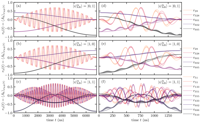
Figure 7: Bloch trajectories for the reduced state of cavities A and B. Only those components $r_{k}(t)=\Braket{\mathsf{A}_{k}}_{\mathsf{\rho}_{\mathrm{AB}}(t)}$ in the generalized Bloch vectors are depicted that show significant changes in time. The opaque, solid lines correspond to the Bloch vector trajectories of $\mathsf{\rho}_{\mathrm{AB}}(t)$ obtained by tracing out transmon C for the dynamics under the two-tone protocol (left column) and the three-tone protocol (right column) as shown in Fig. 2. The dotted lines correspond to the Bloch vector trajectories obtained for a dynamics with the effective Hamiltonian (31), which is only defined on the reduced system of the two cavities.

In this appendix we reconstruct — based on the numerical data shown in Fig. 2 — an effective Hamiltonian that correctly describes the dynamics of the reduced subsystem of the two cavities. As we will show, this Hamiltonian works for both the two- and three-tone protocol confirming once more that adding the third drive indeed gives rise to a stronger beamsplitter interaction. This is particularly remarkable given the differences in the correlation dynamics between Fig. 3(a) and (b). The two-tone protocol gives rise to almost unitary dynamics in the reduced subsystem of the two cavities since the transmon stays uncorrelated at all times. In contrast, the three-tone protocol gives rise to correlations between cavities and transmon, cf. Fig. 3, and thus indicates non-unitary dynamics of the reduced subsystem of the cavities.

In the following, we inspect the reduced dynamics of the two cavities. To this end, we introduce the generalized Bloch vector $\boldsymbol{r}(t)=(r_{1}(t),\dots,r_{M^{2}-1}(t))^{\top}$ of the reduced state $\mathsf{\rho}_{\mathrm{AB}}(t)=\mathrm{tr}_{\mathrm{c}}\{\mathsf{\rho}(t)\}$ of cavities A and B,

$$\mathsf{\rho}_{\mathrm{AB}}(t)=\frac{1}{M}\mathsf{\mathbbm{1}}_{M}+\boldsymbol{r}(t)\cdot\boldsymbol{\mathsf{\hat{A}}},$$ (30)

where $M=\dim\{\mathcal{H}_{\mathrm{a}}\otimes\mathcal{H}_{\mathrm{b}}\}$ and $\boldsymbol{\mathsf{\hat{A}}}=(\mathsf{A}_{1},\dots,\mathsf{A}_{M^{2}-1})^{\top}$. Here $\{\mathsf{A}_{1},\dots,\mathsf{A}_{M^{2}-1}\}$ is a basis of traceless, Hermitian $M\times M$ matrices satisfying $\braket{\mathsf{A}_{i},\mathsf{A}_{j}}=\delta_{i,j}$. We choose the generalized Gell-Mann matrices for this basis and order them according to their presentation in Ref. Bertlmann and Krammer (2008). For the numerical simulations presented in Fig. 2, we have $M=25$, hence the generalized Bloch vector $\boldsymbol{r}(t)$ has $25^{2}-1=624$ components. For the effective beamsplitter interaction of the two-tone protocol, cf. Fig. 2(a), many of these components are constant or almost constant and only a small fraction shows a significant time-dependence. The opaque, solid lines in Fig. 7(a)-(c) show the dynamics of those “relevant” components for the initial states $\ket{\psi_{\mathrm{AB}}^{\mathrm{in}}}\in\{\ket{0,1,0},\ket{1,0,0},\ket{1,1,0}\}$ in the bare basis. Figure 7(d)-(e) show the same components for the three-tone protocol, cf. Fig. 2(b). As can be seen, the slowly changing components in Fig. 7(d)-(e) follow a slightly more complex version than their counterparts in panels (a)-(c) but are identical in shape. In contrast, the rapidly oscillating components follow the same envelope in both cases but their oscillations differ. Note the different time scales of the dynamics. The rapid oscillations have actually the same frequency for both the two- and three-tone protocol.

Since there is no immediate procedure to derive an effective Hamiltonian for the subsystem of cavities A and B, we numerically find an effective Hamiltonian that fits the dynamics observed in Fig. 7. The effective Hamiltonian reads

$$\mathsf{H}_{\mathrm{eff}}^{\mathrm{AB}}(t)=-g_{\mathrm{BS}}\left(e^{-\textup{i}\omega_{\mathrm{z}}t}\mathsf{a}\mathsf{b}^{\dagger}+e^{\textup{i}\omega_{\mathrm{z}}t}\mathsf{a}^{\dagger}\mathsf{b}\right)-\frac{\omega_{\mathrm{z}}}{2}\left(\mathsf{a}^{\dagger}\mathsf{a}-\mathsf{b}^{\dagger}\mathsf{b}\right).$$ (31)

For the original two-tone protocol, the two parameters of the effective Hamiltonian (31) are $g_{\mathrm{BS}}/2\pi=$36.9\text{\,}\mathrm{kHz}$$ and $\omega_{\mathrm{z}}/2\pi=$2.625\text{\,}\mathrm{MHz}$$. For the three-tone protocol, the two parameters are $g_{\mathrm{BS}}/2\pi=$165\text{\,}\mathrm{kHz}$$ and $\omega_{\mathrm{z}}/2\pi=$2.625\text{\,}\mathrm{MHz}$$. In both cases, the parameters are obtained by fitting the effective, analytical curves generated by Hamiltonian (31) to the numerical curves of Fig. 7. As expected, the effective beamsplitter interaction $g_{\mathrm{BS}}$ is larger for the three-tone protocol. It increases by a factor $4.47$ which roughly matches the decrease in protocol duration (factor $4.54$). Interestingly, the rapidly oscillating components in Fig. 7 can be reproduced by the same frequency $\omega_{\mathrm{z}}/2\pi=$2.625\text{\,}\mathrm{MHz}$$ for both protocols. It exactly matches the relative Stark shift for $\omega_{a}$ and $\omega_{b}$ in the original two-tone protocol, which can be calculated from the parameters in Table 1 and Eq. (6) via

$$(\omega_{2}-\omega_{1})-(\omega_{\mathrm{b}}-\omega_{\mathrm{a}})=$2.625\text{\,}\mathrm{MHz}$.$$ (32)

This readily explains the difference between Eq. (5) and Eq. (31), as the latter describes the dynamics in the frame set by Hamiltonian (II.1), i.e., in a rotating frame where both cavities A and B have vanishing level splittings $\omega_{\mathrm{a}}$ and $\omega_{\mathrm{b}}$. However, this frame does not capture the Stark shifts $\omega_{\mathrm{a}}\rightarrow\tilde{\omega}_{\mathrm{a}}$ and $\omega_{\mathrm{b}}\rightarrow\tilde{\omega}_{\mathrm{b}}$ induced by the drives on the transmon. In consequence, both cavities have still non-vanishing level splittings in the rotating frame and hence the non-vanishing $\omega_{\mathrm{z}}$ in Eq. (31).

The fact that $\omega_{\mathrm{z}}$ is identical for the two- and three-tone protocol is surprising, since the third drive could, in principle, give rise to different individual Stark shifts of $\omega_{\mathrm{a}}$ and $\omega_{\mathrm{b}}$. However, the relative Stark shift is identical for both protocols. This might be viewed as another numerical confirmation of the effective theory presented in Eqs. (29a) and (29b), namely that the first two tones are exclusively responsible for activating the beamsplitter interaction via Eq. (6) while the third tone exclusively adds the cavity-transmon sideband transitions.

Appendix B Floquet calculation of the beamsplitter rate

The Floquet results shown in Fig. 5 of the main text were obtained by using the method developed in Ref. Zhang et al. (2019), which we briefly describe here. Note that the following Floquet treatment is an approximate method to estimate the beamsplitter rate.

As a first step, we start from the Hamiltonian in Eq. (II.1) and switch to the rotating frame at the frequency $\omega_{1}$ of driving field 1. This leads to the Hamiltonian

$$\mathsf{H}(t) =\mathsf{H}_{\mathrm{c}}(t)+(\omega_{\mathrm{a}}-\omega_{1})\mathsf{a}^{\dagger}\mathsf{a}+(\omega_{\mathrm{b}}-\omega_{1})\mathsf{b}^{\dagger}\mathsf{b}$$

$$\quad+g_{\mathrm{a}}\left(\mathsf{a}\mathsf{c}^{\dagger}+\mathsf{a}^{\dagger}\mathsf{c}\right)+g_{\mathrm{b}}\left(\mathsf{b}\mathsf{c}^{\dagger}+\mathsf{b}^{\dagger}\mathsf{c}\right),$$ (33)

$$\mathsf{H}_{\mathrm{c}}(t) =(\omega_{\mathrm{c}}-\omega_{1})\mathsf{c}^{\dagger}\mathsf{c}-\frac{\alpha_{\mathrm{c}}}{2}\mathsf{c}^{\dagger}\mathsf{c}^{\dagger}\mathsf{c}\mathsf{c}$$

$$\quad+\left(\Omega_{1}+\Omega_{2}e^{-\textup{i}\omega_{21}t}+\Omega_{3}e^{-\textup{i}\omega_{31}t}\right)\mathsf{c}^{\dagger}$$

$$\quad+\left(\Omega_{1}^{*}+\Omega_{2}^{*}e^{\textup{i}\omega_{21}t}+\Omega_{3}^{*}e^{\textup{i}\omega_{31}t}\right)\mathsf{c}.$$ (34)

Here we consider time-independent drive amplitudes $\Omega_{1,2,3}$, and we define $\omega_{21}$ and $\omega_{31}$ to be $\omega_{21}=\omega_{2}-\omega_{1}$, $\omega_{31}=\omega_{3}-\omega_{1}$.

The key idea of the method is to treat the cavity-transmon couplings in Eq. (B) above perturbatively, but treat the drives non-perturbatively using Floquet theory. To apply Floquet theory, we require $\omega_{21}$ to be commensurate with $\omega_{31}$. In practice, this is done by keeping finite number of digits for the numerical values of the drive frequencies. In the results shown in Fig. 5, we round the drive frequencies in unit of MHz to the closest integer. For instance, $\omega_{2}/2\pi$ is rounded to $7050\text{\,}\mathrm{MHz}$. After this, we find the smallest positive integers $p$ and $q$ such that the ratio of $\omega_{21}$ and $\omega_{31}$ is given by $p/q$. Then the transmon Hamiltonian $\mathsf{H}_{\mathrm{c}}$ in Eq. (34) is time-periodic, namely,

$$\mathsf{H}_{\mathrm{c}}(t+2\pi/\omega_{\mathrm{H}})=\mathsf{H}_{\mathrm{c}}(t),\quad\omega_{\mathrm{H}}=\omega_{21}/p=\omega_{31}/q.$$ (35)

Because $\mathsf{H}_{\mathrm{c}}(t)$ is periodic in time, by Floquet theorem, there is a set of Floquet eigenstates associated with $\mathsf{H}_{\mathrm{c}}(t)$ — analog to stationary eigenstates for static Hamiltonians. These Floquet states can be written in the form

$$\psi_{m}(t) =e^{-\textup{i}\epsilon_{m}t}u_{m}(t),$$ (36)

where $\epsilon_{m}$ is the quasienergy and $u_{m}$ is called the Floquet mode which has the same periodicity as the Hamiltonian, i.e., $u_{m}(t+2\pi/\omega_{\mathrm{H}})=u_{m}(t)$.

As derived in Ref. Zhang et al. (2019), to leading order in the coupling strengths $g_{\mathrm{a}},g_{\mathrm{b}}$, the cavity-cavity beamsplitter rate when the transmon is in the $m$th Floquet state is given by the following formula

$$g_{\mathrm{BS},m} =g_{\mathrm{a}}^{*}g_{\mathrm{b}}\sum_{n}\sum_{K}\left[\frac{\mathsf{c}_{mn,K+1}(\mathsf{c}^{\dagger})_{nm,-K}}{\omega_{\mathrm{b}}-\omega_{1}+K\omega_{\mathrm{H}}+\epsilon_{mn}}\right.$$

$$\quad+\left.\frac{(\mathsf{c}^{\dagger})_{mn,-K}\mathsf{c}_{nm,K+1}}{-\omega_{\mathrm{b}}+\omega_{1}-K\omega_{\mathrm{H}}+\epsilon_{mn}}\right],$$ (37)

where $\epsilon_{mn}=\epsilon_{m}-\epsilon_{n}$ and where $\mathsf{c}_{mn,K}$ is the $K$th Fourier component of the matrix element of the transmon operator $\mathsf{c}$ between its Floquet modes $u_{m}$ and $u_{n}$,

$$\mathsf{c}_{mn,K}=\frac{\omega_{\mathrm{H}}}{2\pi}\int_{0}^{2\pi/\omega_{\mathrm{H}}}\langle u_{m}(t)|\mathsf{c}|u_{n}(t)\rangle e^{-\textup{i}K\omega_{\mathrm{H}}t}\mathrm{d}t.$$ (38)

To obtain the Floquet results in Fig. 5, we set $m=0$ in Eq. (B), which corresponds to the Floquet state that adiabatically connects to the transmon ground state without the drive. Near the sideband resonance, we find that using the dressed frequency of cavity B — approximately given by $\omega_{\mathrm{b}}+g_{\mathrm{b}}^{2}/(\omega_{\mathrm{b}}-\omega_{\mathrm{c}})$ — in place of bare frequency $\omega_{\mathrm{b}}$ in Eq. (B) produces a better agreement with the time-domain numerical results. To obtain the error bars in Fig. 5, we simply shift $\omega_{\mathrm{b}}/2\pi$ by $\pm$1\text{\,}\mathrm{MHz}$$. This allows us to explore the sensitivity of the beamsplitter rate on the distance to the sideband resonance.

Appendix C Constructing two- and three-tone protocols with minimal transmon excitation

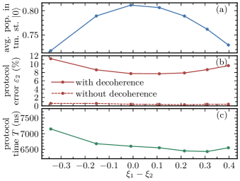
Figure 8: Error analysis for various two-tone protocols based on the difference $\xi_{1}-\xi_{2}$ of the normalized amplitudes $\xi_{1}$ and $\xi_{2}$ but conditioned by $\xi_{1}\xi_{2}=0.126$. Panel (a) shows the average bare ground state population of the transmon (without decoherence) for the respective protocol, cf. Eq. (39). Panel (b) shows the protocol error $\varepsilon_{2}$ with and without decoherence, while (c) shows the corresponding protocol duration $T$.

In this appendix, we examine how to engineer two- and three-tone protocols with minimal excitation of the transmon. While one might suppose that this only helps in improving robustness with respect to $T_{1}^{\mathrm{c}}$, recall that with fewer excitations in higher transmon levels, also fewer coherences with respect to these levels occur. To identify such protocols, we need to find drive parameters for which the Floquet state — to which the transmon is dynamically transferred by switching the drive on and off — is closest to the bare ground state. To this end, we compare various two-tone protocols under the constraint of identical $|\xi_{1}\xi_{2}|$, where $\xi_{k}=\Omega_{k}/\delta_{k}$ is the normalized amplitude and $\delta_{k}=\omega_{k}-\omega_{\mathrm{c}}$ a detuning. Note that despite $|\xi_{1}\xi_{2}|$ being the main quantity that defines the beamsplitter rate $g_{\mathrm{BS}}$, cf. Eq. (5), and thus the protocol duration $T$, the individual physical amplitudes $\Omega_{1}$ and $\Omega_{2}$ and thus individual normalized amplitudes $\xi_{1}$ and $\xi_{2}$ can still be chosen differently.

Figure 8(a) shows the average bare ground state population of the transmon, defined via

$$\frac{1}{TM^{2}}\sum_{n_{\mathrm{a}},n_{\mathrm{b}}=0}^{M-1}\int_{0}^{T}\mathrm{d}t\left\llangle\ket{0}\bra{0}\bigg{|}\mathrm{tr}_{\mathrm{ab}}\left\{\mathcal{D}_{t,0}\left[\mathsf{\rho}_{n_{\mathrm{a}},n_{\mathrm{b}},0}\right]\right\}\right\rrangle,$$ (39)

as a function of the difference $\xi_{1}-\xi_{2}$ for the two-tone protocol. As can be seen, the average transmon ground state population is maximal if $\xi_{1}-\xi_{2}\approx 0$, i.e., both drives have roughly the same normalized amplitude. All these two-tone protocols have coherent errors $<0.6\%$, see dashed line in Fig. 8(b). Once decoherence is taken into account, the protocols with larger average transmon ground state population have smaller protocol errors $\varepsilon_{2}$ (solid line). The minimal error roughly occurs for $\xi_{1}-\xi_{2}=0$. Due to the constraint of identical $|\xi_{1}\xi_{2}|$, the protocol durations $T$ are very similar (albeit not identical), cf. Fig. 8(c).

While Fig. 8 shows results for one particular choice of $|\xi_{1}\xi_{2}|$, one might conjecture that weaker values — and thus longer protocol durations — lead to larger average transmon ground state population and hence more robustness with respect to transmon decoherence. However, our observations indicate that being faster is always advantageous. Thus, in order to find the protocol with best resistance against decoherence, the primary goal should be to be fast and the secondary goal should be to stay on average as close as possible to the bare transmon ground state. This statement should hold for any three-tone protocol as well, since the average bare ground state population decreases only slightly once the third drive is turned on, decreasing for instance from $0.73$ to $0.70$ for the protocols discussed in Fig. 2. Figure 8 thus represents a good starting point to find suitable two-tone protocols that can subsequently be turned into high fidelity three-tone protocols.

References

- Acín et al. (2018) A. Acín, I. Bloch, H. Buhrman, T. Calarco, C. Eichler, J. Eisert, D. Esteve, N. Gisin, S. J. Glaser, F. Jelezko, S. Kuhr, M. Lewenstein, M. F. Riedel, P. O. Schmidt, R. Thew, A. Wallraff, I. Walmsley, and F. K. Wilhelm, New J. Phys. 20, 080201 (2018).
- Nielsen and Chuang (2000) M. A. Nielsen and I. L. Chuang, Quantum computation and quantum information (Cambridge University Press, Cambridge, 2000).
- Georgescu et al. (2014) I. M. Georgescu, S. Ashhab, and F. Nori, Rev. Mod. Phys. 86, 153 (2014).
- Degen et al. (2017) C. L. Degen, F. Reinhard, and P. Cappellaro, Rev. Mod. Phys. 89, 035002 (2017).
- D’Alessandro (2007) D. D’Alessandro, Introduction to Quantum Control and Dynamics, 1st ed. (Chapman and Hall/CRC, 2007).
- Glaser et al. (2015) S. J. Glaser, U. Boscain, T. Calarco, C. P. Koch, W. Köckenberger, R. Kosloff, I. Kuprov, B. Luy, S. Schirmer, T. Schulte-Herbrüggen, D. Sugny, and F. K. Wilhelm, Eur. Phys. J. D 69, 279 (2015).
- Mao et al. (1986) J. Mao, T. Mareci, K. Scott, and E. Andrew, J. Magn. Reson. 70, 310 (1986).
- Murdoch et al. (1987) J. B. Murdoch, A. H. Lent, and M. R. Kritzer, J. Magn. Reson. 74, 226 (1987).
- Tannor and Rice (1985) D. J. Tannor and S. A. Rice, J. Chem. Phys. 83, 5013 (1985).
- Peirce et al. (1988) A. P. Peirce, M. A. Dahleh, and H. Rabitz, Phys. Rev. A 37, 4950 (1988).
- Kosloff et al. (1989) R. Kosloff, S. Rice, P. Gaspard, S. Tersigni, and D. Tannor, Chem. Phys. 139, 201 (1989).
- Müller et al. (2011) M. M. Müller, D. M. Reich, M. Murphy, H. Yuan, J. Vala, K. B. Whaley, T. Calarco, and C. P. Koch, Phys. Rev. A 84, 042315 (2011).
- Watts et al. (2015) P. Watts, J. Vala, M. M. Müller, T. Calarco, K. B. Whaley, D. M. Reich, M. H. Goerz, and C. P. Koch, Phys. Rev. A 91, 062306 (2015).
- Caneva et al. (2011) T. Caneva, T. Calarco, and S. Montangero, Phys. Rev. A 84, 022326 (2011).
- Goerz et al. (2015) M. H. Goerz, K. B. Whaley, and C. P. Koch, EPJ Quantum Technol. 2, 21 (2015).
- Wittler et al. (2021) N. Wittler, F. Roy, K. Pack, M. Werninghaus, A. S. Roy, D. J. Egger, S. Filipp, F. K. Wilhelm, and S. Machnes, Phys. Rev. Applied 15, 034080 (2021).
- Skinner and Gershenzon (2010) T. E. Skinner and N. I. Gershenzon, J. Magn. Reson. 204, 248 (2010).
- Sørensen et al. (2018) J. J. W. H. Sørensen, M. O. Aranburu, T. Heinzel, and J. F. Sherson, Phys. Rev. A 98, 022119 (2018).
- Machnes et al. (2018) S. Machnes, E. Assémat, D. Tannor, and F. K. Wilhelm, Phys. Rev. Lett. 120, 150401 (2018).
- Günther et al. (2021) S. Günther, N. A. Petersson, and J. L. DuBois, AVS Quantum Sci. 3, 043801 (2021).
- Khaneja et al. (2005) N. Khaneja, T. Reiss, C. Kehlet, T. Schulte-Herbrüggen, and S. J. Glaser, J. Magn. Reson. 172, 296 (2005).
- Goerz et al. (2019) M. H. Goerz, D. Basilewitsch, F. Gago-Encinas, M. G. Krauss, K. P. Horn, D. M. Reich, and C. P. Koch, SciPost Phys. 7, 80 (2019).
- Palao et al. (2008) J. P. Palao, R. Kosloff, and C. P. Koch, Phys. Rev. A 77, 063412 (2008).
- Palao et al. (2013) J. P. Palao, D. M. Reich, and C. P. Koch, Phys. Rev. A 88, 053409 (2013).
- Koch (2016) C. P. Koch, J. Phys.: Condens. Matter 28, 213001 (2016).
- Dolde et al. (2014) F. Dolde, V. Bergholm, Y. Wang, I. Jakobi, B. Naydenov, S. Pezzagna, J. Meijer, F. Jelezko, P. Neumann, T. Schulte-Herbrüggen, J. Biamonte, and J. Wrachtrup, Nat. Commun. 5, 3371 (2014).
- Waldherr et al. (2014) G. Waldherr, Y. Wang, S. Zaiser, M. Jamali, T. Schulte-Herbrüggen, H. Abe, T. Ohshima, J. Isoya, J. F. Du, P. Neumann, and J. Wrachtrup, Nature 506, 204 (2014).
- Heeres et al. (2017) R. W. Heeres, P. Reinhold, N. Ofek, L. Frunzio, L. Jiang, M. H. Devoret, and R. J. Schoelkopf, Nat. Commun. 8, 94 (2017).
- Wu et al. (2020) X. Wu, S. L. Tomarken, N. A. Petersson, L. A. Martinez, Y. J. Rosen, and J. L. DuBois, Phys. Rev. Lett. 125, 170502 (2020).
- Werninghaus et al. (2021) M. Werninghaus, D. J. Egger, F. Roy, S. Machnes, F. K. Wilhelm, and S. Filipp, npj Quantum Inf. 7, 14 (2021).
- Omran et al. (2019) A. Omran, H. Levine, A. Keesling, G. Semeghini, T. T. Wang, S. Ebadi, H. Bernien, A. S. Zibrov, H. Pichler, S. Choi, J. Cui, M. Rossignolo, P. Rembold, S. Montangero, T. Calarco, M. Endres, M. Greiner, V. Vuletić, and M. D. Lukin, Science 365, 570 (2019).
- Nöbauer et al. (2015) T. Nöbauer, A. Angerer, B. Bartels, M. Trupke, S. Rotter, J. Schmiedmayer, F. Mintert, and J. Majer, Phys. Rev. Lett. 115, 190801 (2015).
- Poggiali et al. (2018) F. Poggiali, P. Cappellaro, and N. Fabbri, Phys. Rev. X 8, 021059 (2018).
- Larrouy et al. (2020) A. Larrouy, S. Patsch, R. Richaud, J.-M. Raimond, M. Brune, C. P. Koch, and S. Gleyzes, Phys. Rev. X 10, 021058 (2020).
- Titum et al. (2021) P. Titum, K. Schultz, A. Seif, G. Quiroz, and B. D. Clader, npj Quantum Inf. 7, 53 (2021).
- Braunstein (1998) S. L. Braunstein, Phys. Rev. Lett. 80, 4084 (1998).
- Braunstein and van Loock (2005) S. L. Braunstein and P. van Loock, Rev. Mod. Phys. 77, 513 (2005).
- Gottesman et al. (2001) D. Gottesman, A. Kitaev, and J. Preskill, Phys. Rev. A 64, 012310 (2001).
- Joshi et al. (2021) A. Joshi, K. Noh, and Y. Y. Gao, Quantum Sci. Technol. 6, 033001 (2021).
- Gyenis et al. (2021) A. Gyenis, A. Di Paolo, J. Koch, A. Blais, A. A. Houck, and D. I. Schuster, arXiv:2106.10296 (2021).
- Terhal et al. (2020) B. M. Terhal, J. Conrad, and C. Vuillot, Quantum Sci. Technol. 5, 043001 (2020).
- Mirrahimi et al. (2014) M. Mirrahimi, Z. Leghtas, V. V. Albert, S. Touzard, R. J. Schoelkopf, L. Jiang, and M. H. Devoret, New J. Phys. 16, 045014 (2014).
- Michael et al. (2016) M. H. Michael, M. Silveri, R. T. Brierley, V. V. Albert, J. Salmilehto, L. Jiang, and S. M. Girvin, Phys. Rev. X 6, 031006 (2016).
- Albert et al. (2019) V. V. Albert, S. O. Mundhada, A. Grimm, S. Touzard, M. H. Devoret, and L. Jiang, Quantum Sci. Technol. 4, 035007 (2019).
- Ofek et al. (2016) N. Ofek, A. Petrenko, R. Heeres, P. Reinhold, Z. Leghtas, B. Vlastakis, Y. Liu, L. Frunzio, S. M. Girvin, L. Jiang, M. Mirrahimi, M. H. Devoret, and R. J. Schoelkopf, Nature 536, 441 (2016).
- Grimm et al. (2020) A. Grimm, N. E. Frattini, S. Puri, S. O. Mundhada, S. Touzard, M. Mirrahimi, S. M. Girvin, S. Shankar, and M. H. Devoret, Nature 584, 205 (2020).
- Hu et al. (2019) L. Hu, Y. Ma, W. Cai, X. Mu, Y. Xu, W. Wang, Y. Wu, H. Wang, Y. P. Song, C.-L. Zou, S. M. Girvin, L.-M. Duan, and L. Sun, Nature Physics 15, 503 (2019).
- Gertler et al. (2021) J. M. Gertler, B. Baker, J. Li, S. Shirol, J. Koch, and C. Wang, Nature 590, 243 (2021).
- DiVincenzo (2000) D. P. DiVincenzo, Fortschr. Phys. 48, 771 (2000).
- Poletto et al. (2012) S. Poletto, J. M. Gambetta, S. T. Merkel, J. A. Smolin, J. M. Chow, A. D. Córcoles, G. A. Keefe, M. B. Rothwell, J. R. Rozen, D. W. Abraham, C. Rigetti, and M. Steffen, Phys. Rev. Lett. 109, 240505 (2012).
- Chow et al. (2012) J. M. Chow, J. M. Gambetta, A. D. Córcoles, S. T. Merkel, J. A. Smolin, C. Rigetti, S. Poletto, G. A. Keefe, M. B. Rothwell, J. R. Rozen, M. B. Ketchen, and M. Steffen, Phys. Rev. Lett. 109, 060501 (2012).
- Gaebler et al. (2016) J. P. Gaebler, T. R. Tan, Y. Lin, Y. Wan, R. Bowler, A. C. Keith, S. Glancy, K. Coakley, E. Knill, D. Leibfried, and D. J. Wineland, Phys. Rev. Lett. 117, 060505 (2016).
- Ballance et al. (2016) C. J. Ballance, T. P. Harty, N. M. Linke, M. A. Sepiol, and D. M. Lucas, Phys. Rev. Lett. 117, 060504 (2016).
- Josse et al. (2004) V. Josse, A. Dantan, A. Bramati, M. Pinard, and E. Giacobino, Phys. Rev. Lett. 92, 123601 (2004).
- Masada et al. (2015) G. Masada, K. Miyata, A. Politi, T. Hashimoto, J. L. O'Brien, and A. Furusawa, Nat. Photonics 9, 316 (2015).
- Reagor et al. (2013) M. Reagor, H. Paik, G. Catelani, L. Sun, C. Axline, E. Holland, I. M. Pop, N. A. Masluk, T. Brecht, L. Frunzio, M. H. Devoret, L. Glazman, and R. J. Schoelkopf, Appl. Phys. Lett. 102, 192604 (2013).
- Ma et al. (2021) W.-L. Ma, S. Puri, R. J. Schoelkopf, M. H. Devoret, S. Girvin, and L. Jiang, Sci. Bull. 66, 1789 (2021).
- Gambetta et al. (2017) J. M. Gambetta, J. M. Chow, and M. Steffen, npj Quantum Inf. 3, 2 (2017).
- Kjaergaard et al. (2020) M. Kjaergaard, M. E. Schwartz, J. Braumüller, P. Krantz, J. I.-J. Wang, S. Gustavsson, and W. D. Oliver, Annu. Rev. Condens. Matter Phys. 11, 369 (2020).
- Rosenblum et al. (2018) S. Rosenblum, Y. Y. Gao, P. Reinhold, C. Wang, C. J. Axline, L. Frunzio, S. M. Girvin, L. Jiang, M. Mirrahimi, M. H. Devoret, and R. J. Schoelkopf, Nat. Commun. 9, 652 (2018).
- Chou et al. (2018) K. S. Chou, J. Z. Blumoff, C. S. Wang, P. C. Reinhold, C. J. Axline, Y. Y. Gao, L. Frunzio, M. H. Devoret, L. Jiang, and R. J. Schoelkopf, Nature 561, 368 (2018).
- Gao et al. (2019) Y. Y. Gao, B. J. Lester, K. S. Chou, L. Frunzio, M. H. Devoret, L. Jiang, S. M. Girvin, and R. J. Schoelkopf, Nature 566, 509 (2019).
- Gao et al. (2018) Y. Y. Gao, B. J. Lester, Y. Zhang, C. Wang, S. Rosenblum, L. Frunzio, L. Jiang, S. M. Girvin, and R. J. Schoelkopf, Phys. Rev. X 8, 021073 (2018).
- Koch et al. (2007) J. Koch, T. M. Yu, J. Gambetta, A. A. Houck, D. I. Schuster, J. Majer, A. Blais, M. H. Devoret, S. M. Girvin, and R. J. Schoelkopf, Phys. Rev. A 76, 042319 (2007).
- Zhang et al. (2019) Y. Zhang, B. J. Lester, Y. Y. Gao, L. Jiang, R. J. Schoelkopf, and S. M. Girvin, Phys. Rev. A 99, 012314 (2019).
- Breuer and Petruccione (2002) H.-P. Breuer and F. Petruccione, The theory of open quantum systems, 1st ed. (Oxford University Press, 2002).
- Nelder and Mead (1965) J. A. Nelder and R. Mead, Comput. J. 7, 308 (1965).
- Konnov and Krotov (1999) A. I. Konnov and V. F. Krotov, Autom. Rem. Contr. 60, 1427 (1999).
- Reich et al. (2012) D. M. Reich, M. Ndong, and C. P. Koch, J. Chem. Phys. 136, 104103 (2012).
- Palao and Kosloff (2003) J. P. Palao and R. Kosloff, Phys. Rev. A 68, 062308 (2003).
- Goerz et al. (2014) M. H. Goerz, D. M. Reich, and C. P. Koch, New J. Phys. 16, 055012 (2014).
- Reich (2014) D. Reich, Efficient Characterisation and Optimal Control of Open Quantum Systems - Mathematical Foundations and Physical Applications, Ph.D. thesis, University of Kassel (2014).
- Note (1) Note the self-consistent nature of Eq. (17\@@italiccorr) where the update of the field at time on the left-hand side depends on the very same field and time on the right-hand side. In practice, this is solved by discretizing the time grid sufficiently fine such that for the update at time step on the left-hand side the corresponding values for fields (and states) at time step on the right-hand side are a good approximation. See Ref. Palao and Kosloff (2003) for further details.
- (74) QDYN library, www.qdyn-library.net.
- (75) S. G. Johnson, The NLopt nonlinear-optimization package, www.github.com/stevengj/nlopt.
- Henderson and Vedral (2001) L. Henderson and V. Vedral, J. Phys. A 34, 6899 (2001).
- Note (2) The optimizations have been carried out without frequency truncation in order to keep the number of iterations sufficiently small.
- Note (3) We assume the transmon to be in the ground state, thus replacing by in Eq. (29b\@@italiccorr).
- Zhang et al. (2021) Y. Zhang, J. C. Curtis, C. S. Wang, R. J. Schoelkopf, and S. M. Girvin, arXiv:2106.09112 (2021).
- Wang et al. (2022) C. Wang, X. Li, H. Xu, Z. Li, J. Wang, Z. Yang, Z. Mi, X. Liang, T. Su, C. Yang, G. Wang, W. Wang, Y. Li, M. Chen, C. Li, K. Linghu, J. Han, Y. Zhang, Y. Feng, Y. Song, T. Ma, J. Zhang, R. Wang, P. Zhao, W. Liu, G. Xue, Y. Jin, and H. Yu, npj Quantum Inf. 8, 3 (2022).
- Place et al. (2021) A. P. M. Place, L. V. H. Rodgers, P. Mundada, B. M. Smitham, M. Fitzpatrick, Z. Leng, A. Premkumar, J. Bryon, A. Vrajitoarea, S. Sussman, G. Cheng, T. Madhavan, H. K. Babla, X. H. Le, Y. Gang, B. Jäck, A. Gyenis, N. Yao, R. J. Cava, N. P. de Leon, and A. A. Houck, Nat. Commun. 12, 1779 (2021).
- Bertlmann and Krammer (2008) R. A. Bertlmann and P. Krammer, J. Phys. A: Math. Theor. 41, 235303 (2008).