Inverse design of gradient-index volume multimode converters

Abstract

Graded-index optical elements are capable of shaping light precisely and in very specific ways. While classical freeform optics uses only a two-dimensional domain such as the surface of a lens, recent technological advances in laser manufacturing offer promising prospects for the realization of arbitrary three-dimensional graded-index volumes, i.e. transparent dielectric substrates with voxel-wise modified refractive index distributions. Such elements would be able to perform complex light transformations on compact scales.

Here we present an algorithmic approach for computing 3D graded-index devices, which utilizes numerical beam propagation and error reduction based on gradient descent. We present solutions for millimeter-sized elements addressing important tasks in photonics: a mode sorter, a photonic lantern and a multimode intensity beam shaper. We further discuss suitable cost functions for all designs to be used in the algorithm. The 3D graded-index designs are spatially smooth and require a relatively small refractive index range in the order of $10^{-2}$, which is within the reach of direct laser writing manufacturing processes such as two-photon polymerization.

1 Introduction

Light has become one of the most powerful and versatile tools. It is an important medium for transporting information, either between communicating partners or from an object under investigation to a detector in imaging applications. Light also plays a key role in laser-based manufacturing processes, such as welding, cutting and direct laser lithography.

However, as recently highlighted [1, 2, 3], exploiting the full physical potential of light requires solutions for its highly specific and custom shaping. For example, increasing the telecommunication bandwidth demands directing photonic signals from many single mode fibers into a single multi-core or multimode fiber with high efficiency [4]. Likewise, efficiently exploiting the high optical power of industrial lasers requires to reshape their often unsuitable native mode profiles [5, 6].

In any case, the restructuring of light should ideally take up only little space. To this end, the processing of dielectric materials such as glasses or polymers with ultra-fast lasers has opened promising routes towards the creation of three-dimensional, miniaturized light shapers [7]. A variety of devices such as photonic lanterns, beam combiners and mode multiplexers made from glass-embedded waveguide arrangements have been successfully demonstrated and are making their way towards commercialization. Such waveguides are formed by translating a femtosecond laser focus through a glass volume along the desired guiding paths, along which the refractive index of the glass is permanently modified. Whilst undoubtedly powerful, devices using waveguides as “building blocks” are nevertheless limited in the sense that they don’t fully exploit all degrees of freedom of a volume. Ideally, one would like to have the power of arbitrarily changing the entire three-dimensional refractive index distribution at the microscale. Progress towards the fabrication of such 3D gradient index materials for optical wavelengths has been recently reported using two-photon polymerization [8, 9] and 3D printed glass optics [10]. Likewise, the computational design of 3D gradient index optics in order to shape arbitrary transverse beam profiles is continuously advancing. In Ref. [11], the authors use an irradiance mapping scheme relying on geometric optics, which is found by employing algorithms used in optimal mass transport problems, on top of which they run a multiplane Gerchberg-Saxton-like algorithm in order to account for diffraction. The proposed algorithm, however, has some constraints with regards to the smoothness and continuity of input/output functions. Furthermore, it has so far only been demonstrated for single-mode shaping, that is sculpting a specific coherent output field from a single coherent input beam.

Here we propose a new algorithmic approach for the design of 3D gradient index devices. Unlike previous methods for designing gradient index or freeform optics, we refrain from using tools used in ray-optical designs. Instead, we employ an approach related to machine learning, i.e., numerical beam propagation in conjunction with suitable cost functions that are optimized using error back-propagation and gradient descent. We demonstrate the effectiveness and versatility of our approach by computing a variety of highly miniaturized 3D gradient index designs that perform key tasks in integrated photonics. After a detailed explanation of our computational method and suitable cost functions in section 2, we present solutions for three application cases in section 3.

Firstly, we find a solution for a mode sorter of only 2.5 mm length, which is capable of specifically mapping 45 Gaussian input beams onto the Hermite-Gaussian modes of a multimode fiber with an average conversion efficiency of 98.6%. Secondly, we design an equally small photonic lantern, which couples light from 45 Gaussian inputs unspecifically into a multimode fiber with 99.2% efficiency. Finally, we present a highly miniaturized beam shaper of only 0.5 mm length, which turns the irradiance profile of a monochromatic $50\,\textrm{\textmu m}$-diameter multimode fiber source into a speckle-free square of $60\,\textrm{\textmu m}$ side length.

All presented designs exhibit smooth 3D refractive index modulations within a dynamic range of about $10^{-2}$ and are therefore feasible for experimental realization using 2-photon polymerization [8].

2 Inverse design algorithm

In the following, we present an algorithm that allows to design gradient-index structures for the conversion of a set $\{u_{n}\}_{1\leq n\leq N}$ of $N$ mutually incoherent transverse input modes to another set of output modes $\{v_{n}\}_{1\leq n\leq N}$, according to various cost functions depending on the application.

We follow a typical inverse design approach by first defining a forward model propagating the input modes from their definition plane $z_{in}$ to the destination plane $z_{out}$, through a structure of refractive index contrast $\Delta\textrm{RI}(x,y,z)$ that is initially unknown and will be updated iteratively. We then define different cost functions for several classes of multimode beam shaping problems and present a generic error backpropagation algorithm to compute $\Delta\textrm{RI}$ gradients. Finally, we combine these different stages into a simple gradient descent iteration scheme to solve $\Delta\textrm{RI}$ and eventually apply some constraints to it.

2.1 Forward model

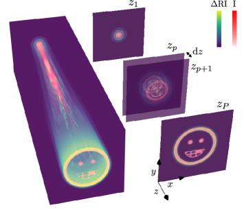
Figure 1: Illustration of a Gaussian to smiley gradient index mode conversion along with its discrete formulation, consisting of $P$ planes separated by a small distance $\mathrm{d}z$.

We consider a refractive index distribution $\Delta\textrm{RI}(x,y,z)$ of finite extent in a rectangular coordinate system ($O,x,y,z$), $z$ being the direction of propagation of the incoming laser modes $\{u_{n}\}_{1\leq n\leq N}$. The wavelength of the input and output modes in vacuum is denoted $\lambda_{0}$. The RI volume is discretized into $P$ transverse planes located at axial positions $\{z_{p}\}_{1\leq p\leq P}$ separated by a small distance $\mathrm{d}z$, as illustrated in Figure 1. The transverse resolution is denoted $(\mathrm{d}x,\mathrm{dy})$. The refractive index $n_{b}$ of the medium between these different planes is assumed to be the same as for the bulk material, while each plane holds a phase mask proportional to the local $\Delta\textrm{RI}$ distribution and to $\mathrm{d}z$:

$$\Delta\varphi_{p}(x,y)=\frac{2\pi}{\lambda_{0}}\Delta\textrm{RI}(x,y,z_{p})\mathrm{d}z,$$ (1)

for $p\in\{1,\dots,P\}$. Then, the numerical propagation of the input modes $\{u_{n}\}$ through the $\Delta\textrm{RI}$ distribution is achieved with the standard split-step beam propagation method (BPM), alternating propagation in a uniform medium of refractive index $n_{b}$ and multiplication by a phase mask defined according to Eq. (1). A symmetric split-step scheme is enforced simply by defining the input plane position $z_{in}$ at a distance $\mathrm{d}z/2$ before $z_{1}$ and the output plane position $z_{out}$ at $\mathrm{d}z/2$ after $z_{P}$.

For propagating between planes we use the well-known angular spectrum (AS) method:

$$u_{\perp(z+\textrm{d}z)} =\textsc{IFFT}\left(\textsc{FFT}{\left(u_{\perp z}\right)}\times\exp{\left(i2\pi\mathrm{d}z\sqrt{\frac{n_{b}^{2}}{\lambda_{0}^{2}}-f_{x}^{2}-f_{y}^{2}}\right)}\right)$$ (2)

where FFT and IFFT refer to the two-dimensional fast Fourier transform and its inverse. A detailed pseudocode description of the forward model, propagating a N-vector of input modes $U_{in}$ defined in the input plane $z_{in}$ to a N-vector of output modes $U_{out}$ in the destination plane $z_{out}$, is given in Algorithm 1 of Appendix A.

2.2 Cost functions and errors for different classes of problems

Depending on the beam shaping application, different cost functions can be defined, which quantify the quality of the light transform by a single scalar value $C$. Here, we consider two types of cost functions, either distances that we want to minimize to zero, or functions of merit representing a physical quantity that we want to maximize.

In order to keep the notations simple, we still name $\{u_{n}\}_{1\leq n\leq N}$ the elements of the N-vector $U_{out}$ representing the input modes propagated to the plane $z_{out}$. We note $\bar{U}=(\partial C/\partial u_{n})_{1\leq n\leq N}$ the error vector whose elements $\{\bar{u}_{n}\}$ represent the variation of the cost function with respect to each propagated mode $u_{n}$. The $\{u_{n}\}$ being complex-valued, it is important to define some consistent algebraic rules for achieving such differentiation. We use the complex representation defined in [12] along with the corresponding differentiation rules. It is worth noting that other representations and derivation rules based on Wirtinger calculus can be used [13], but they should lead to the same result in the end when error computations with respect to real-valued parameters (e.g. phases) are performed. Using such rules, we see that the errors $\{\bar{u}_{n}\}$ have the same dimension as the input and output modes $\{u_{n}\}$ and $\{v_{n}\}$, so we call them error modes in the following. Table 1 lists a few interesting cost functions and associated error modes for different beam shaping problems, which we describe in the following.

beam shaping class	cost function C	error $\mathbf{\bar{U}}$
multimode matching	$\min\sum\limits_{n=1}^{N}\iint|u_{n}-v_{n}|^{2}$	$\bar{u}_{n}=2(u_{n}-v_{n})$
multimode 1–1 power coupling	$\max\sum\limits_{n=1}^{N}{\left|\iint{v_{n}^{*}u_{n}}\right|^{2}}$	$\bar{u}_{n}=2\left(\iint{v_{n}^{*}u_{n}}\right)v_{n}$
multimode N–N power coupling	$\max\sum\limits_{n=1}^{N}\sum\limits_{l=1}^{N}{\left|\iint{v_{l}^{*}u_{n}}\right|^{2}}$	$\bar{u}_{n}=2\sum\limits_{l=1}^{N}{\left(\iint{v_{l}^{*}u_{n}}\right)}v_{l}$
multimode intensity shaping	$\min\iint\left(I_{S}-I_{T}\right)^{2}$	$\bar{u}_{n}=4(I_{S}-I_{T})u_{n}$

Table 1: Examples of cost functions and associated errors for different classes of beam shaping problems.

The first cost function we refer to as "multimode matching" is a squared $l_{2}$ distance between the modes $\{u_{n}\}$ and $\{v_{n}\}$ with a one-to-one correspondence. We call it that way because, in the case of lossless designs, its application matches rigorously the wavefront matching method introduced in a previous article [14] in the context of mode multiplexing with planar lightwave circuits (PLC). Indeed, a lossless design implies the conservation of $\|u_{n}\|_{2}^{2}$ during $u_{n}$ propagation, which leads to a simpler expression for the error vector components:

$$\bar{u}_{n}=-2v_{n}.$$ (3)

We see that, up to a constant factor, the error modes correspond to the target modes $\{v_{n}\}$. In this case, the application of the backpropagation of errors we develop in the next subsection leads exactly to the wavefront matching method presented in [14], even if the authors obtain this result with an alternative reasoning.

If the phase offset between each mode pair $u_{n}$ and $v_{n}$ is not relevant for the multiplexing problem, a different cost function can be introduced that we name "multimode 1–1 power coupling". This time, the cost function represents the sum of overlap integrals between input and target modes and must therefore be maximized. We note that the error vector components differ from the simplified expression of multimode matching given in Eq. (3) only by a complex constant factor corresponding to the overlap integrals and by a sign which just results from the difference between minimization and maximization problems. This slight modification pre-aligns the relative constant phases between each $u_{n}$ and $v_{n}$, which can sometimes help to reduce the inverse design complexity.

We introduce a third cost function named "multimode N–N power coupling", which aims at maximizing the total power coupling between the input set of modes $\{u_{n}\}$ and the target modes $\{v_{n}\}$ without requiring a one-to-one mapping. This metric can be useful for applications such as incoherent combining of a set of modes into a multimode fiber, or for space division multiplexing (SDM) in telecommunications [4], as we will illustrate in the numerical results section. Compared to the multimode 1–1 power coupling metric, this one gives much more flexibility to the optimization algorithm since it allows for mapping each input mode onto an arbitrary linear combination of target modes $\{v_{n}\}$. Usually, this additional degree of freedom results in smoother and more symmetrical designs.

Finally, we introduce a cost function named "multimode intensity shaping", which allows to shape the total intensity distribution $I_{S}$ of mutually incoherent input modes $\{u_{n}\}$ into a desired target intensity shape $I_{T}$. For this particular beam shaping application, it is not necessary to define a set of target modes $\{v_{n}\}$, as only $I_{T}$ is relevant. Moreover, the $\{u_{n}\}$ being mutually incoherent, their time-averaged total intensity profile is simply given by:

$$I_{S}=\sum\limits_{n=1}^{N}{|u_{n}|^{2}}.$$ (4)

In the following, we describe the backpropagation algorithm that allows to compute the gradients $\partial C/\partial\Delta\textrm{RI}$ for any cost function $C$ in a unified fashion, starting from its associated and case specific error vector $\bar{U}$.

2.3 Backpropagation of errors

Algorithm 2 of Appendix A describes the backpropagation of the error modes vector $\bar{U}$ in order to compute the refractive index gradients associated to each plane $\nabla_{\textrm{RI}}[p]=\partial C/\partial\Delta\textrm{RI}[p]$ in a reverse fashion. Here, the term "backpropagation" refers to the traditional definition found in machine learning, where the chain rule is applied in order to compute the partial derivatives of the cost function with respect to some parameters of interest backwards. Following the complex representation of errors defined in [12], it appears that this procedure also corresponds exactly to the physical backpropagation of the error modes through the optical system.

2.4 Optimization algorithm

The optimization algorithm relies on gradient descent and can be summarized in the following steps:

1. Initialize $\Delta\textrm{RI}$.

2. Compute the propagated modes $U_{out}$ by calling the function propagate_forward (Algorithm 1) on the input modes $U_{in}$.

3. Eval $C$ and $\bar{U}$, associated to a particular beam shaping problem, using the propagated modes $U_{out}$.

4. Compute the refractive index gradients $\nabla_{\textrm{RI}}$ by calling backpropagate_gradient (Algorithm 2) on the error modes $\bar{U}$.

5. Update $\Delta\textrm{RI}$ with a gradient step along $\nabla_{\textrm{RI}}$.

6. Enforce constraints on $\Delta\text{RI}$.

7. If $C$ satisfies a stopping criterion then return $\Delta\textrm{RI}$, otherwise go to step 2.

Concerning step 1, we often initialize $\Delta\textrm{RI}$ to zero even if it is worth mentioning that some better initialization schemes could be used [11]. A clever initialization can help to achieve a faster convergence in case the propagated modes through a constant refractive index medium have a very low spatial overlap with the target modes.

Concerning step 5, one needs to introduce a constant step size, small enough to avoid divergence, or use an adaptive learning rate method. Of course the direction of the gradient step has to be chosen consistently, depending on whether the cost function has to be minimized or maximized.

Concerning step 6, it is worth mentioning that enforcing constraints right after performing gradient steps finds a mathematical justification in the proximal algorithms framework[15]. A typical constraint that we wish to apply is the restriction of $\Delta\textrm{RI}$ to a fixed interval, in order to satisfy manufacturing constraints for instance.

3 Numerical results

In this section, we present some numerical results that illustrate the versatility of the optimization algorithm in addressing different beam shaping problems involving fiber optics. We aim at designing fully integrated devices of only millimeter length, which do not require any collimation or focusing of the input and output beams. The refractive index contrast required to realize some of the proposed devices may be difficult to achieve with current glass or polymer gradient manufacturing processes, but the main aim of this work is to propose a proof of concept and give an idea of the objectives to be reached so that these types of devices can be industrially manufactured.

3.1 Hermite-Gaussian mode sorter

The first system we design is a Hermite-Gaussian (HG) mode sorter, inspired by recent work [16], where the authors perform a conversion of 210 modes from a set of Gaussian input beams arranged in a triangle to a set of co-propagating HG modes. Mode sorters are a proposed solution for increasing the telecommunication bandwidth by exploiting the concept of selective mode-division multiplexing, i.e., coupling many signals into a few-mode or multimode fiber [7] with control of the particular excitation of a given output mode.

In [16], the HG conversion is performed by only 7 phase masks separated by free space propagation and is implemented experimentally by a multi-pass cavity formed by a spatial light modulator (SLM) and a flat mirror. The algorithm used in article [16] is equivalent to a coordinate descent formulation of the wavefront matching method presented in [14]. It is important to underline that this complex transformation is only made possible by a clever one-to-one mapping between the cartesian coordinates of a Gaussian mode in the triangle arrangement and the order $(m,n)$ of the corresponding HG output mode. With so few phase patterns, any other arrangement would lead to poor convergence of the mode transformation.

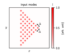
Figure 2: Triangle arrangement for the 45 Gaussian input modes.

In order to limit the computational resources to something reasonable, we restrict the mode conversion to 45 modes, which still includes interesting applications for telecommunications [17]. We set the working wavelength $\lambda_{0}=1.55\,\textrm{\textmu m}$ and use Gaussian modes of waist $\omega_{in}=5.2\,\textrm{\textmu m}$ as inputs, typical of single mode fibers (SMF-28). Figure 2 shows the triangle arrangement of the 45 input modes, with a separation parameter $\Delta=4\,\omega_{in}$. For the outputs, we use the HG representation of standard graded-index multimode fibers’ eigenmodes, with a maximum refractive index contrast $dn_{\textrm{max}}=15\times 10^{-3}$ between the core and the cladding as in [17]. With a mode solver [18], we compute the eigenmodes for such a fiber profile and estimate the value $\omega_{out}=7.7\,\textrm{\textmu m}$ for the HG output modes’ waist. To each of the 45 input modes, we assign one of the output fiber HG eigenmodes according to the mapping described in  [16]. In short, if the Cartesian position of an input mode in the triangle arrangement (in a $45^{\circ}$ rotated frame compared to Figure 2) is expressed as $(m\Delta,n\Delta)$, then the associated output mode is $\textrm{HG}_{m,n}$.

In simulation, the device is represented by a $512\times 512\times 250$ array, the first two dimensions corresponding to the transverse planes and the third one to the plane index. The bulk refractive index used for the propagation between planes is set to $n_{b}=1.444$ corresponding to fused silica. The transverse resolution is set to $\mathrm{d}x=\mathrm{d}y=0.65\,\textrm{\textmu m}$ and the separation between planes is $\mathrm{d}z=10\,\textrm{\textmu m}$, leading to a total device length of 2.5 mm. At first glance, the axial resolution may appear a bit low for BPM accuracy, but we verify afterwards that it is feasible, by linearly interpolating the final simulated RI profile with a better resolution $\mathrm{d}z=0.5\,\textrm{\textmu m}$ and by propagating the input modes through it. Limiting the number of planes in the simulation is crucial because we need to store all the input modes at each plane during the forward pass (Algorithm 1) in order to be able to compute a gradient afterwards (Algorithm 2). Even with single-precision complex numbers, this already requires 23.6 GB of memory allocation.

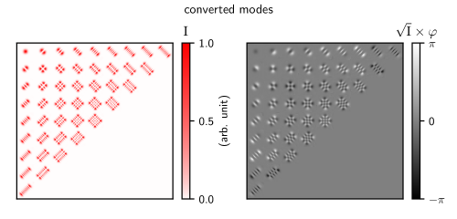
Figure 3: Intensity and phase patterns of the 45 created HG modes. The average conversion efficiency is 98.6%.

In order to achieve this 45-mode conversion, we run 1500 iterations of the optimization algorithm using the multimode 1-1 power coupling cost function defined in table 1. After each iteration, we force the values of $\Delta\textrm{RI}$ to stay within a range of $12\times 10^{-3}$, which is slightly smaller than the RI contrast $dn_{\textrm{max}}$ required to guide the output HG modes. We observed that enforcing stricter constraints on $\Delta\textrm{RI}$ causes losses in the mode conversion due to the device’s inability to strongly guide the small modes involved. In the end of the iterations, the cost function reaches the value $C\simeq 44.37$, corresponding to an average conversion efficiency of 98.6% per mode. As in [16], we introduce the $N\times N$ transfer matrix $T$ of the device, whose elements $t_{ij}=\int{v_{i}^{*}u_{j}}$ are the overlaps between the output and the propagated input modes. For this particular device, we find that the auto-correlation matrix $X=|T^{\dagger}T|$ has a largest off-diagonal term $X_{\textrm{max}}=-46.16$ dB, corresponding to an extremely small crosstalk between modes. The intensity and phase of each converted mode are shown in Figure 3, where we recognize almost perfectly shaped HG modes.

Figure 4: Evolution of the simulated transverse RI profile sections through the center of the mode sorter device along the propagation direction, for the multimode HG conversion.

Figure 4 illustrates horizontal and vertical sections through the center of the mode converter, indicating a very smooth evolution of the refractive index along the propagation direction. The input facet $z=z_{in}$ defines multiple waveguides for each of the 45 Gaussian input modes while the end facet $z=z_{out}$ defines a single larger waveguide holding the co-propagating HG modes. In between, the waveguides are merged by the algorithm in order to achieve the desired mode to mode mapping.

3.2 Photonic lanterns

Photonic lanterns are optical components allowing for a low-loss conversion between a set of fundamental modes belonging to independent single-mode waveguides and a set of high-order modes belonging to a common multimode waveguide [19].

The functional difference between a photonic lantern and a mode sorter as discussed previously is that the lantern is an non-selective device that does not aim for a pre-defined mode-to-mode mapping. The only goal is to couple as much power into the set of modes supported by the output fiber, while preserving mode orthogonality. Such objects are usually fabricated by tapering single-mode waveguides together or by femtosecond laser writing and they find applications in astrophotonics [20] and SDM [21] for telecommunications.

The empirical adiabatic merging of different fiber cores gives rise to super-modes by evanescent coupling, but it is challenging to ensure that this process is lossless and that the final modal content exactly matches a unitary superposition of modes belonging to a given few-mode or multimode fiber. Assuming that we can control the RI distribution as we wish, we will show that the multimode N-N power coupling metric proposed in Table 1 is perfectly adapted to overcome this difficulty. If the target waveguide was a graded-index multimode fiber whose eigenmodes are Hermite-Gaussian, then the HG mode sorter presented previously would already be an appropriate solution. However, it is not necessarily possible to find a Cartesian representation for the eigenmodes of an arbitrary fiber profile, one example are the linearly polarized (LP) modes of a step-index fiber.

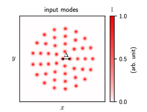
Figure 5: Concentric ring arrangement for the 45 input modes of the photonic lantern.

Here, we still define the working wavelength $\lambda_{0}=1.55\,\textrm{\textmu m}$ and the bulk refractive index $n_{b}=1.444$. The device is represented by a $350\times 350\times 250$ array, with the same transverse and axial resolution as before, leading again to a total device length of 2.5 mm. Concerning the input modes, we still use the fundamental Gaussians of single-mode fibers with $\omega_{in}=\textrm{5.2 \textmu m}$, but this time with a concentric ring arrangement which has been shown to lead to the best coupling efficiency for a photonic lantern design with tapered waveguides [22]. Figure 5 represents the concentric ring arrangement for 45 input modes, with a separation parameter $\Delta=4\,\omega_{in}$ as before.

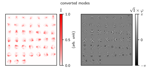
Figure 6: Intensity and phase profiles of the converted modes.

Concerning the output modes, we use the first 45 Laguerre-Gaussian (LG) modes with $\omega_{out}=\textrm{7.7 \textmu m}$, using their real-valued representation with circular and radial nodal lines. For the multimode N-N power coupling optimization, the exact base representation is not relevant since it allows for a linear rearrangement of the modes, but we find it nicer for visualizing the intensity profiles later on.

After only 300 iterations of the optimization algorithm, we reach a total power coupling efficiency of 99.2%. As in [16], we define insertion losses (IL) and mode dependent losses (MDL) of the device using the singular values $\{\sigma_{i}\}_{1\leq i\leq N}$ resulting from the singular value decomposition (SVD) of the transfer matrix $T=U\Sigma V^{\dagger}$:

$$\textrm{IL}= \frac{1}{N}\sum\limits_{i=1}^{N}|\sigma_{i}|^{2}$$ (5)

$$\textrm{MDL}= \frac{\max{\{|\sigma_{i}|^{2}\}}}{\min{\{|\sigma_{i}|^{2}\}}}.$$ (6)

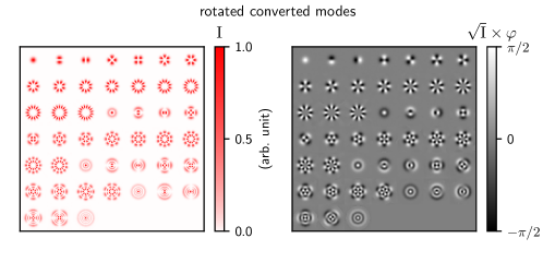
Figure 7: Intensity and phase profiles of the converted modes rotated by the unitary matrix $UV^{\dagger}$ resulting from the SVD.

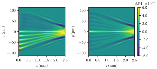
Figure 8: Transverse RI profiles through the center of the photonic lantern design. The total power coupling efficiency is 99.2%.

For this particular device, we obtain $\textrm{IL}=0.035$ dB, $\textrm{MDL}=0.097$ dB and a maximum crosstalk $X_{\textrm{max}}=-46.5$ dB, corresponding to an auto-correlation matrix $X=|T^{\dagger}T|$ almost equal to the identity matrix. Figure 6 shows that the converted modes look very different from the LG modes defining the output basis, but Figure 7 shows that, since $\Sigma\simeq\mathbb{I}$, the original LG modes can be recovered by rotating the converted modes with the unitary matrix $UV^{\dagger}$ resulting from the SVD decomposition of the transfer matrix $T$.

Finally, Figure 8 shows that the computed design is very smooth and symmetrical, resembling a tapering of several single-mode waveguides, thus truly deserving the name photonic lantern. Our results prove that our method is able to engineer integrated photonic lantern devices in a very precise fashion, with perfectly controlled input and output modes. To our knowledge, this inverse design approach is new in this context.

3.3 Multimode intensity shaping

Finally, we would like to treat the application of shaping the intensity profile of a light source emitting many mutually incoherent modes. This class of beam shaping has importance in various fields, such as digital holography or laser material processing, where the native intensity profile of the light source is often not ideal for the task at hand. The associated cost function is called “multimode intensity shaping” in Table 1. In a recent article, we have used the same optimization metric to find two cascaded phase patterns for shaping the intensity profile of a light emitting diode (LED) [23]. Here, we aim at realizing the same kind of intensity shaping with a volumetric gradient index design, starting from the eigenmodes of a step-index fiber with a diameter of $50\,\textrm{\textmu m}$ and $\textrm{NA}=0.1$.

In simulation, we use $\lambda_{0}=0.640\,\textrm{\textmu m}$ as the working wavelength and $n_{b}=1.457$ as the refractive index of fused silica at this wavelength. With such parameters, a mode solver finds 158 eigenmodes for this particular step-index fiber. We further assume that each input mode contributes with the same optical power. The device is represented by a $256\times 256\times 50$ array with a transverse resolution $\mathrm{d}x=\mathrm{d}y=0.5\,\textrm{\textmu m}$ and a separation between planes $\mathrm{d}z=10\,\textrm{\textmu m}$. This corresponds to a total device length of only 0.5 mm. As previously, we validate our sampling choice by linearly interpolating the final RI profile along the z-direction at a finer sampling interval of $\mathrm{d}z=0.5\,\textrm{\textmu m}$, followed by a simulated readout of the gradient index design.

As desired output, we define a square target intensity profile $I_{T}$ with a side length of $60\,\textrm{\textmu m}$. The square is modeled as the Cartesian product of two 1D supergaussian profiles of order 20 to provide smooth edges.

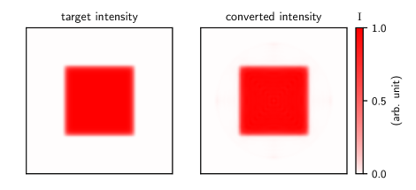
Figure 9: Theoretical target intensity profile and converted multimode intensity profile obtained by simulation.

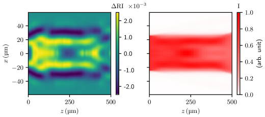
Figure 10: RI profile and total intensity profile in the central x-z-plane of the beam shaper.

For this simulation, we restrict the $\Delta\textrm{RI}$ range to $5\times 10^{-3}$ and we also enforce a smooth design by Fourier filtering the 3D RI profile with a sharp low-pass filter at each iteration. This Fourier filtering corresponds to a projection of the RI distribution on a set of band-limited functions, which makes it a theoretically valid proximal operator [15]. Here, we enforce the smallest details in the RI profile to be around $4\,\textrm{\textmu m}$. After 1500 iterations, even under these constraints, we reach an almost perfect intensity conversion as illustrated in Figure 9.

Figure 10 shows the RI profile and the total intensity evolution of the beam along the propagation direction. We observe that the obtained RI profile is very smooth, and its limited $\Delta\textrm{RI}$ range makes it already manufacturable with commercial 3D printers with polymers [24], even if it may require some slice stitching in order to reach the full 0.5 mm length. We also see that the beam is guided in the computed RI structure while its intensity is continuously shaped into the desired profile. The fact that the total length is 5 times shorter for this multimode shaping device than for the previous mode sorter or photonic lantern shows that multimode intensity shaping requires in general much less degrees of freedom than individual or collective mode matching. The same conclusion holds for discrete designs such as presented in Refs. [23] and [16].

4 Conclusion

We have demonstrated a powerful and versatile computational method to design millimeter-range integrated devices performing several important multimode light transformations. Different cost functions were introduced for solving particular mode multiplexing or intensity shaping problems, but the optimization approach is stated in such a general way that any other user-defined cost function would fall within the scope presented here. The presented designs can already be manufactured with the available two-photon polymerization technologies and we can envision that their realization in a glass material will also be accessible in the coming years. Our work could be extended further to include broad-spectrum or multicolor sources, or to account for light polarization, which would cover many more applications in optics with fully integrated designs.

Appendix A Algorithms

Both forward and backward propagation rely on the angular spectrum method which is implemented by the $\textsc{as\_prop}(u,\lambda_{0},n_{b},\mathrm{d}z)$ function, $u$ being the transverse mode to propagate, $\lambda_{0}$ the wavelength in vacuum, $n_{b}$ the bulk refractive index and $\mathrm{d}z$ the propagation distance.

A.1 Forward model

Algorithm 1 Forward model

$\mathbf{Constants:}$ $\lambda_{0}$, $n_{b}$, $\mathrm{d}z$

$\mathbf{Inputs:}$ $U_{in}$ a $N$-vector of input modes at plane $z_{in}$

$\mathbf{Inputs:}$ $\Delta\mathrm{RI}$ a $P$-vector of 2D refractive index distributions

$\mathbf{Outputs:}$ $U_{out}$ a $N$-vector of modes propagated to plane $z_{out}$

$\mathbf{Outputs:}$ $S$ a $P$-vector of $N$-vectors of modes stored at each plane

procedure propagate_forward($U_{in}$, $\Delta\mathrm{RI}$)

     $S\leftarrow\textsc{Vector}(\mathrm{typeof}(U_{in}),P)$ $\triangleright$ allocating a P-vector of N-vectors of modes

     $U_{out}\leftarrow\textsc{copy}(U_{in})$ $\triangleright$ copy allocation

     $U_{out}\leftarrow\textsc{as\_prop.}(U_{out},\lambda_{0},n_{b},\mathrm{d}z/2)$ $\triangleright$ propagating modes to plane $z_{1}$

     $U_{out}\leftarrow U_{out}\cdot\exp{(i\frac{2\pi}{\lambda_{0}}\Delta\mathrm{RI}[1])}$ $\triangleright$ crossing the $1$^st refractive index mask forward

     $S[1]\leftarrow U_{out}$ $\triangleright$ storing modes at plane $z_{1}$

     for $p=2\,\mathbf{to}\,P$ do

         $U_{out}\leftarrow\textsc{as\_prop.}(U_{out},\lambda_{0},n_{b},\mathrm{d}z)$ $\triangleright$ propagating modes to the next plane

         $U_{out}\leftarrow U_{out}\cdot\exp{(i\frac{2\pi}{\lambda_{0}}\Delta\mathrm{RI}[p])}$ $\triangleright$ crossing $p$^th refractive index mask forward

         $S[p]\leftarrow U_{out}$ $\triangleright$ storing modes at plane $z_{p}$

     end for

     $U_{out}\leftarrow\textsc{as\_prop.}(U_{out},\lambda_{0},n_{b},\mathrm{d}z/2)$ $\triangleright$ propagating modes to plane $z_{out}$

     return $(U_{out},S)$

end procedure

Algorithm 1 describes the forward model in a more formal way. The set of input modes is represented by an N-vector $U_{in}$, each of its elements being a two-dimensional array storing a particular mode distribution $\{u_{n}\}_{1\leq n\leq N}$ in plane $z_{in}$. The 3D refractive index distribution is represented by a P-vector $\Delta\textrm{RI}$ whose elements are two dimensional arrays representing the refractive index profiles at each plane $z_{p}$. The function propagate_forward propagates the vector of modes $U_{in}$ through the 3D refractive index distribution $\Delta\textrm{RI}$, plane by plane, and returns a new vector $U_{out}$ of propagated modes to the final plane $z_{out}$. It also returns $S$, a stored copy of each input mode at each plane, which will be crucial for computing the refractive index gradients later on. In order to avoid verbose loops over the mode index, we introduced a broadcasting notation by appending a dot (.) after as_prop function name, meaning that we apply this function to each element of the vector passed as first argument, and that the return type is also a vector of same length. Similarly, the pointwise multiplication of each vector component by a common phase mask has been represented by a dot $(\cdot)$ operator. Finally, it is worth mentioning that these vector representations for modes and RI distributions are useful for a concise and functional pseudo-code description, but that in practice they should rather be represented by contiguous multidimensional arrays for better efficiency.

A.2 Error backpropagation

Algorithm 2 RI gradient computation

$\mathbf{Constants:}$ $\lambda_{0}$, $n_{b}$, $\mathrm{d}z$

$\mathbf{Inputs:}$ $\bar{U}$ a N-vector of error modes associated to a cost function at plane $z_{out}$

$\mathbf{Inputs:}$ $S$ a $P$-vector of $N$-vectors of modes stored at each plane

$\mathbf{Inputs:}$ $\Delta\mathrm{RI}$ a $P$-vector of 2D refractive index distributions

$\mathbf{Outputs:}$ $\nabla_{\mathrm{RI}}$ a P-vector of RI gradients

procedure backpropagate_gradient($\bar{U}$, $S$, $\Delta\mathrm{RI}$)

     $\nabla_{\mathrm{RI}}\leftarrow\textsc{similar}(\Delta\mathrm{RI})$ $\triangleright$ allocating an uninitialized RI gradient vector

     $\bar{U}\leftarrow\textsc{as\_prop.*}(\bar{U},\lambda_{0},n_{b},\mathrm{d}z/2)$ $\triangleright$ backpropagating errors to plane $z_{P}$

     for $p=P\,\mathbf{to}\,2$ do

         $\nabla_{\mathrm{RI}}[p]\leftarrow\frac{2\pi}{\lambda_{0}}\Im{\left(\sum\limits_{k=1}^{N}(S^{*}[p]\cdot\bar{U})[k]\right)}$ $\triangleright$ Computing the $p$^th RI gradient

         $\bar{U}\leftarrow\bar{U}\cdot\exp{(-i\frac{2\pi}{\lambda_{0}}\Delta\mathrm{RI}[p])}$ $\triangleright$ crossing the $p$^th refractive index mask backward

         $\bar{U}\leftarrow\textsc{as\_prop.*}(\bar{U},\lambda_{0},n_{b},\mathrm{d}z)$ $\triangleright$ backpropagating errors to the previous plane

     end for

     $\nabla_{\mathrm{RI}}[1]\leftarrow\frac{2\pi}{\lambda_{0}}\Im{\left(\sum\limits_{k=1}^{N}(S^{*}[1]\cdot\bar{U})[k]\right)}$ $\triangleright$ Computing the $1$^st RI gradient

     return $\nabla_{\mathrm{RI}}$

end procedure

The function backpropagate_gradient can be seen as a mirrored version of the function propagate_forward defined in algorithm 1, where each operator has been replaced by its adjoint (hermitian conjugate). The star (^∗) appended after the as_prop function name denotes this adjoint operation. Additionally, we see that the gradient computations $\nabla_{\textrm{RI}}[p]$ are performed using the information $S[p]$ stored in each plane during the forward pass. These gradient expressions can be derived from the set of rules presented in [12].

In case of a tight grid extension, which is always desirable in order to save memory consumption, some Fourier artifacts can easily appear due to a portion of unguided light reaching the edges. This problem can be overcome simply by adding some absorbing boundary conditions on a thin region before the grid edges. In the forward model, this can for instance be implemented by applying an absorption mask on the propagating modes in conjunction with the phase mask multiplication. It is worth mentioning that in the backward pass, it must then also be treated as an absorption mask for the backpropagating modes, as the adjoint operator needs to be considered (and not the inverse).

Funding.

The work is funded by the FWF (I3984-N36).

References

- [1] Halina Rubinsztein-Dunlop, Andrew Forbes, Michael V Berry, Mark R Dennis, David L Andrews, Masud Mansuripur, Cornelia Denz, Christina Alpmann, Peter Banzer, Thomas Bauer, et al. Roadmap on structured light. Journal of Optics, 19(1):013001, 2016.
- [2] Andrew Forbes, Michael de Oliveira, and Mark R Dennis. Structured light. Nature Photonics, 15(4):253–262, 2021.
- [3] Marco Piccardo, Vincent Ginis, Andrew Forbes, Simon Mahler, Asher A Friesem, Nir Davidson, Haoran Ren, Ahmed H Dorrah, Federico Capasso, Firehun T Dullo, et al. Roadmap on multimode light shaping. arXiv preprint arXiv:2104.03550, 2021.
- [4] Benjamin J Puttnam, Georg Rademacher, and Ruben S Luís. Space-division multiplexing for optical fiber communications. Optica, 8(9):1186–1203, 2021.
- [5] Sensen Li, Yulei Wang, Zhiwei Lu, Lei Ding, Pengyuan Du, Yi Chen, Zhenxing Zheng, Dexin Ba, Yongkang Dong, Hang Yuan, et al. High-quality near-field beam achieved in a high-power laser based on SLM adaptive beam-shaping system. Optics Express, 23(2):681–689, 2015.
- [6] Lisa Ackermann, Clemens Roider, and Michael Schmidt. Uniform and efficient beam shaping for high-energy lasers. Optics Express, 29(12):17997–18009, 2021.
- [7] S Gross and MJ Withford. Ultrafast-laser-inscribed 3d integrated photonics: challenges and emerging applications. Nanophotonics, 4(3):332–352, 2015.
- [8] Albertas Žukauskas, Ieva Matulaitienė, Domas Paipulas, Gediminas Niaura, Mangirdas Malinauskas, and Roaldas Gadonas. Tuning the refractive index in 3d direct laser writing lithography: towards grin microoptics. Laser & Photonics Reviews, 9(6):706–712, 2015.
- [9] Christian R Ocier, Corey A Richards, Daniel A Bacon-Brown, Qing Ding, Raman Kumar, Tanner J Garcia, Jorik Van De Groep, Jung-Hwan Song, Austin J Cyphersmith, Andrew Rhode, et al. Direct laser writing of volumetric gradient index lenses and waveguides. Light: Science & Applications, 9(1):1–14, 2020.
- [10] Rebecca Dylla-Spears, Timothy D Yee, Koroush Sasan, Du T Nguyen, Nikola A Dudukovic, Jason M Ortega, Michael A Johnson, Oscar D Herrera, Frederick J Ryerson, and Lana L Wong. 3d printed gradient index glass optics. Science Advances, 6(47):eabc7429, 2020.
- [11] W Minster Kunkel and James R Leger. Numerical design of three-dimensional gradient refractive index structures for beam shaping. Optics Express, 28(21):32061–32076, 2020.
- [12] Alden S. Jurling and James R. Fienup. Applications of algorithmic differentiation to phase retrieval algorithms. Journal of the Optical Society of America A, 31(7):1348–1359, Jul 2014.
- [13] Praneeth Chakravarthula, Yifan Peng, Joel Kollin, Henry Fuchs, and Felix Heide. Wirtinger holography for near-eye displays. ACM Transactions on Graphics (TOG), 38(6):1–13, 2019.
- [14] Yohei Sakamaki, Takashi Saida, Toshikazu Hashimoto, and Hiroshi Takahashi. New optical waveguide design based on wavefront matching method. Journal of Lightwave Technology, 25(11):3511–3518, 2007.
- [15] Neal Parikh and Stephen Boyd. Proximal algorithms. Foundations and Trends in Optimization, 1(3):127–239, 2014.
- [16] Nicolas K Fontaine, Roland Ryf, Haoshuo Chen, David T Neilson, Kwangwoong Kim, and Joel Carpenter. Laguerre-gaussian mode sorter. Nature Communications, 10(1):1–7, 2019.
- [17] Nicolas K Fontaine, Roland Ryf, Haoshuo Chen, Steffen Wittek, Jiaxiong Li, JC Alvarado, JE Antonio Lopez, Mark Cappuzzo, Rose Kopf, AI Tate, et al. Packaged 45-mode multiplexers for a graded index fiber. In 2018 European Conference on Optical Communication (ECOC), pages 1–3. IEEE, 2018.
- [18] Arman B Fallahkhair, Kai S Li, and Thomas E Murphy. Vector finite difference modesolver for anisotropic dielectric waveguides. Journal of Lightwave Technology, 26(11):1423–1431, 2008.
- [19] Timothy A Birks, I Gris-Sánchez, Stephanos Yerolatsitis, SG Leon-Saval, and Robert R Thomson. The photonic lantern. Advances in Optics and Photonics, 7(2):107–167, 2015.
- [20] Barnaby Norris and Joss Bland-Hawthorn. Astrophotonics: The rise of integrated photonics in astronomy. Optics and Photonics News, 30(5):26–33, 2019.
- [21] Sergio G Leon-Saval, Nicolas K Fontaine, Joel R Salazar-Gil, Burcu Ercan, Roland Ryf, and Joss Bland-Hawthorn. Mode-selective photonic lanterns for space-division multiplexing. Optics Express, 22(1):1036–1044, 2014.
- [22] Nicolas K Fontaine, Roland Ryf, Joss Bland-Hawthorn, and Sergio G Leon-Saval. Geometric requirements for photonic lanterns in space division multiplexing. Optics Express, 20(24):27123–27132, 2012.
- [23] Nicolas Barré and Alexander Jesacher. Holographic beam shaping of partially coherent light. arXiv preprint arXiv:2110.05083, 2021.
- [24] Xavier Porte, Niyazi Ulas Dinc, Johnny Moughames, Giulia Panusa, Caroline Juliano, Muamer Kadic, Christophe Moser, Daniel Brunner, and Demetri Psaltis. Direct (31)d laser writing of graded-index optical elements. Optica, 8(10):1281–1287, Oct 2021.