Abstract

We will study in details the scalar potential of the Supersymmetric $SU(3)_{C}\otimes SU(3)_{L}\otimes U(1)_{N}$ Model where we introduce the anti-sextet, and without the anti-sextet, in our analyses of all masses of the usual scalar sector.

The Scalar Potential of Supersymmetric $SU(3)_{C}\otimes SU(3)_{L}\otimes U(1)_{N}$ Model

PACS number(s): 12.60. Jv

Keywords: Supersymmetric models

1 Introduction

Models with the following gauge symmetry

$$SU(3)_{C}\otimes SU(3)_{L}\otimes U(1)_{N}$$ (1)

are known as $3-3-1$ for short. They are interesting possibilities for the physics at the TeV scale [1, 2, 3, 4].

The charge operator in the $SU(3)_{L}$ generators,

$$\frac{Q}{e} = \frac{1}{2}(\lambda_{3}-\vartheta\lambda_{8})+N\,\ I_{3\times 3},$$ (2)

where the $\vartheta$ and $N$ are parameters defining differents representation contents and $\lambda_{3}$, $\lambda_{8}$ are the diagonal generators of $SU(3)$ given by

$$\lambda_{3}=\left(\begin{array}[]{ccc}+1&0&0\\ 0&-1&0\\ 0&0&0\end{array}\right),\,\ \lambda_{8}=\frac{1}{\sqrt{3}}\left(\begin{array}[]{ccc}+1&0&0\\ 0&+1&0\\ 0&0&-2\end{array}\right).$$ (9)

The model presented in Ref. [2], with $\vartheta=\sqrt{3}$, the Eq.(2) become

$$\frac{Q}{e} = \left(\begin{array}[]{ccc}N&0&0\\ 0&N-1&0\\ 0&0&N+1\end{array}\right),$$ (13)

and its supersymmetric version has already been considered in Refs. [5, 6, 7, 8]. While the 3-3-1 model of Refs. [3] which corresponds the the case when $\vartheta=(1/\sqrt{3})$, the Eq.(2) become

$$\frac{Q}{e} = \left(\begin{array}[]{ccc}N+\frac{1}{3}&0&0\\ 0&N-\frac{2}{3}&0\\ 0&0&N+\frac{1}{3}\end{array}\right),$$ (17)

his supersymmetric version was built in [9, 10].

In fact, this may be the last symmetry involving the lightest elementary particles: leptons. The lepton sector is exactly the same as in the Standard Model (SM) [11] but now there is a symmetry, at large energies among, say $e^{-}$, $\nu_{e}$ and $e^{+}$ [2] or between $e^{-}$, $\nu_{e}$ and $\nu^{c}_{e}$ [3], therefore there are many model we can construct [4]. Once this symmetry is imposed on the lightest generation and extended to the other leptonic generations it follows that the quark sector must be enlarged by considering heavy exotic charged quarks. It means that some gauge bosons carry lepton and baryon quantum number.

There are two main versions of the 3-3-1 models depending on the embedding of the charge operator in the $SU(3)_{L}$ generators is defined at Eq.(2). In the minimal version, with $\vartheta=\sqrt{3}$, the charge conjugation of the right-handed charged lepton for each generation is combined with the usual $SU(2)_{L}$ doublet left-handed leptons components to form an $SU(3)$ triplet $(\nu_{l_{i}},l_{i},l^{c}_{i})_{L}$. No extra leptons are needed in the mentioned model, and we shall call such model as minimal 3-3-1 model. There are also another possibility where the triplet $(\nu_{l_{i}},l_{i},L^{c}_{i})_{L}$ where $L$ is an extra charged leptons wchich do not mix with the known leptons [12]. We want to remind that there is no right-handed (RH) neutrino in both model. There exists another interesting possibility, where ($\vartheta=1/\sqrt{3}$) a left-handed anti-neutrino to each usual $SU(2)_{L}$ doublet is added to form an $SU(3)$ triplet $(\nu_{l_{i}},l_{i},\nu^{c}_{i})_{L}$, and this model is called the 3-3-1 model with RH neutrinos. The 3-3-1 models have been studied extensively over the last decade.

Although this model coincides at low energies with the SM it explains some fundamental questions that are accommodated, but not explained, in the SM. These questions are:

1. The family number must be a multiple of three in order to cancel anomalies [2, 3];

2. Why $\sin^{2}\theta_{W}<\frac{1}{4}$ is observed;

3. The models have a scalar sector similar to the two Higgs doublets Model, we will review it at App.(A);

4. It is the simplest model that includes bileptons of both types: scalars and vectors ones;

5. It solves the strong $CP$-problem;

6. The model has several sources of CP violation [13, 14].

The supersymmetric version of the 3-3-1 minimal model [2] was done Refs. [5, 6, 7, 8, 15] (MSUSY331). The scalar sector of the minimal 331 model [2] was studied on [16, 17]. When we have presented the MSUSY we have shown the lighest higgs has mass around 124.5 GeV [7].

The scalar sector of 331 model with heavy leptons [12] was studied on [13, 17] and we have studied the Higgs potential with only triplets in supersymmetric case in [15]. The scalar potential in several 331 models was considered in [18, 19, 20, 21].

Recently it was reported a light Higgs boson at the LHC and its value is given by[22]

$$M_{H}=125.09\pm 0.21\,\mathrm{(stat.)}\pm 0.11\,\mathrm{(syst.)}~{}\mathrm{GeV}.$$ (18)

Our goal is to shown that our results presented at [7, 15] is in agreement with the acutal experimental data on scalar sector.

This paper is organized as follows. In Sec. 2 we review the minimal Supersymmetric 3-3-1 Model with $R$-Parity Conservation. Our resutls for the scalar potential with the anti-Sextet is presented in Sec. 3. We done similar analyses with only triplets scalars in Sec. 4. Finally, the last section is devoted to our conclusions. In App.(A) we review the mass spectrum of 3-3-1 Model without Supersymmetry, while in App.(B) we show how to get an analytical expression to our scalar potential in order to compare its expresion with the ones used at 3-3-1 Model.

2 Minimal Supersymmetric 3-3-1 model
(MSUSY331).

This supersymmetric version of the 3-3-1 model given at [2] was presented at [5, 6, 7, 8]. In the minimal 331 model, denoted as m331, the charged leptons gain mass from a triplet and a anti-sextet [2].

In the m331 the scalar sector is composed of three scalar triplets:

$$\eta = \left(\begin{array}[]{c}\eta^{0}\\ \eta^{-}_{1}\\ \eta^{+}_{2}\end{array}\right)\sim({\bf 1},{\bf 3},0),\quad\rho=\left(\begin{array}[]{c}\rho^{+}\\ \rho^{0}\\ \rho^{++}\end{array}\right)\sim({\bf 1},{\bf 3},+1),$$ (25)

$$\chi = \left(\begin{array}[]{c}\chi^{-}\\ \chi^{--}\\ \chi^{0}\end{array}\right)\sim({\bf 1},{\bf 3},-1).$$ (29)

In parenthesis it appears the transformations properties under the respective factors $(SU(3)_{C},SU(3)_{L},U(1)_{N})$. Those scalars, defined at Eq.(29), give masses for all the quarks and the charged leptons are massless. In order to give masses for the charged leptons, at tree level, we have to introduce the following anti-sextet

$$S=\left(\begin{array}[]{ccc}\sigma^{0}_{1}&\frac{h^{+}_{2}}{\sqrt{2}}&\frac{h^{-}_{1}}{\sqrt{2}}\\ \frac{h^{+}_{2}}{\sqrt{2}}&H^{++}_{1}&\frac{\sigma^{0}_{2}}{\sqrt{2}}\\ \frac{h^{-}_{1}}{\sqrt{2}}&\frac{\sigma^{0}_{2}}{\sqrt{2}}&H^{--}_{2}\end{array}\right)\sim({\bf 1},{\bf 6}^{*},0)\,\ .$$ (30)

The scalars get the following vacuum expectation values (VEVs) [7, 8]: When we break the 331 symmetry to the $SU(3)_{C}\otimes U(1)_{EM}$, the scalars get the following vacuum expectation values (VEVs):

$$<\eta>=\left(\begin{array}[]{c}v\\ 0\\ 0\end{array}\right),\quad<\rho>=\left(\begin{array}[]{c}0\\ u\\ 0\end{array}\right),\quad<\chi>=\left(\begin{array}[]{c}0\\ 0\\ w\end{array}\right),$$ (31)

and

$$<S>=\left(\begin{array}[]{ccc}0&0&0\\ 0&0&\frac{z}{\sqrt{2}}\\ 0&\frac{z}{\sqrt{2}}&0\end{array}\right),$$ (32)

where $v=v_{\eta}/\sqrt{2}$, $u=v_{\rho}/\sqrt{2}$, $w=v_{\chi}/\sqrt{2}$ and $z=v_{\sigma_{2}}/\sqrt{2}$.

$$v = \frac{v_{\eta}}{\sqrt{2}}\left(1+\frac{H_{\eta}+\imath F_{\eta}}{|v_{\eta}|}\right),\quad u=\frac{v_{\rho}}{\sqrt{2}}\left(1+\frac{H_{\rho}+\imath F_{\rho}}{|v_{\rho}|}\right),$$

$$w = \frac{v_{\chi}}{\sqrt{2}}\left(1+\frac{H_{\chi}+\imath F_{\chi}}{|v_{\chi}|}\right),\quad z=\frac{v_{\sigma^{0}_{2}}}{\sqrt{2}}\left(1+\frac{H_{\sigma^{0}_{2}}+\imath F_{\sigma^{0}_{2}}}{|v_{\sigma^{0}_{2}}|}\right).$$ (33)

Besides, in order to to cancel chiral anomalies generated by the superpartners of the scalars, we have to add the following higgsinos in the respective anti-multiplets,

$$\tilde{\eta}^{\prime} = \left(\begin{array}[]{c}\tilde{\eta}^{\prime 0}\\ \tilde{\eta}^{\prime+}_{1}\\ \tilde{\eta}^{\prime-}_{2}\end{array}\right)\sim({\bf 1},{\bf 3}^{*},0),\quad\tilde{\rho}^{\prime}=\left(\begin{array}[]{c}\tilde{\rho}^{\prime-}\\ \tilde{\rho}^{\prime 0}\\ \tilde{\rho}^{\prime--}\end{array}\right)\sim({\bf 1},{\bf 3}^{*},-1),$$ (40)

$$\tilde{\chi}^{\prime} = \left(\begin{array}[]{c}\tilde{\chi}^{\prime+}\\ \tilde{\chi}^{\prime++}\\ \tilde{\chi}^{\prime 0}\end{array}\right)\sim({\bf 1},{\bf 3}^{*},+1),$$ (44)

$$\tilde{S}^{\prime}=\left(\begin{array}[]{ccc}\tilde{\sigma}^{\prime 0}_{1}&\frac{\tilde{h}^{\prime-}_{2}}{\sqrt{2}}&\frac{\tilde{h}^{\prime+}_{1}}{\sqrt{2}}\\ \frac{\tilde{h}^{\prime-}_{2}}{\sqrt{2}}&\tilde{H}^{\prime--}_{1}&\frac{\tilde{\sigma}^{\prime 0}_{2}}{\sqrt{2}}\\ \frac{\tilde{h}^{\prime+}_{1}}{\sqrt{2}}&\frac{\tilde{\sigma}^{\prime 0}_{2}}{\sqrt{2}}&\tilde{H}^{\prime++}_{2}\end{array}\right)_{L}\sim({\bf 1},{\bf 6},0).$$ (45)

There are also the scalar partners of the Higgsinos defined in Eqs. (44,45) and we will denote them $\eta^{\prime},\rho^{\prime},\chi^{\prime},S^{\prime}$ [7, 8]. This model was presented at [5, 6, 7, 8].

The usual scalars get the vacuum expectation values (VEVs) defined at Eqs.(32,46). In similar way for the new scalars we can write [7, 8]:

$$v^{\prime} = \frac{v_{\eta^{\prime}}}{\sqrt{2}}\left(1+\frac{H_{\eta^{\prime}}+\imath F_{\eta^{\prime 0}}}{|v_{\eta^{\prime}}|}\right),\quad u^{\prime}=\frac{v_{\rho^{\prime}}}{\sqrt{2}}\left(1+\frac{H_{\rho^{\prime}}+\imath F_{\rho^{\prime}}}{|v_{\rho^{\prime}}|}\right),$$

$$w^{\prime} = \frac{v_{\chi^{\prime}}}{\sqrt{2}}\left(1+\frac{H_{\chi^{\prime}}+\imath F_{\chi^{\prime}}}{|v_{\chi^{\prime}}|}\right),\quad z^{\prime}=\frac{v_{\sigma^{\prime 0}_{2}}}{\sqrt{2}}\left(1+\frac{H_{\sigma^{\prime 0}_{2}}+\imath F_{\sigma^{\prime 0}_{2}}}{|v_{\sigma^{\prime 0}_{2}}|}\right).$$ (46)

It is the complete set of fields in the minimal supersymmetric 3-3-1 model (MSUSY331).

2.1 Genral Superpotential at MSUSY331

The superpotential of our model is given by

$$W=\frac{W_{2}+\bar{W}_{2}}{2}+\frac{W_{3}+\bar{W}_{3}}{3},$$ (47)

with $W_{2}$ having only two chiral superfields while $W_{3}$ has three chiral superfields. The terms allowed by our symmetry are

$$W_{2} = \sum_{i=1}^{3}\mu_{0i}(\hat{L}_{i}\hat{\eta}^{\prime})+\mu_{\eta}(\hat{\eta}\hat{\eta}^{\prime})+\mu_{\rho}(\hat{\rho}\hat{\rho}^{\prime})+\mu_{\chi}(\hat{\chi}\hat{\chi}^{\prime})+\mu_{S}Tr[(\hat{S}\hat{S}^{\prime})],$$ (48)

all the coefficients in the equation above have mass dimension [23] and we also have

$$W_{3} = \sum_{i=1}^{3}\left[\sum_{j=1}^{3}\left(\sum_{k=1}^{3}\lambda_{1ijk}(\epsilon\hat{L}_{i}\hat{L}_{j}\hat{L}_{k})+\lambda_{2ij}(\epsilon\hat{L}_{i}\hat{L}_{j}\hat{\eta})+\lambda_{3ij}(\hat{L}_{i}\hat{S}\hat{L}_{j})\right)+\lambda_{4i}(\epsilon\hat{L}_{i}\hat{\chi}\hat{\rho})\right]$$ (49)

$$+ f_{1}(\epsilon\hat{\rho}\hat{\chi}\hat{\eta})+f_{2}(\hat{\chi}\hat{S}\hat{\rho})+f_{3}(\hat{\eta}\hat{S}\hat{\eta})+f_{4}\epsilon_{ijk}\epsilon_{lmn}\hat{S}_{il}\hat{S}_{jm}\hat{S}_{kn}+f^{\prime}_{1}(\epsilon\hat{\rho}^{\prime}\hat{\chi}^{\prime}\hat{\eta}^{\prime})+f^{\prime}_{2}(\hat{\chi}^{\prime}\hat{S}^{\prime}\hat{\rho}^{\prime})$$

$$+ f^{\prime}_{3}(\hat{\eta}^{\prime}\hat{S}^{\prime}\hat{\eta}^{\prime})+f^{\prime}_{4}\epsilon_{ijk}\epsilon_{lmn}\hat{S}^{\prime}_{il}\hat{S}^{\prime}_{jm}\hat{S}^{\prime}_{kn}+\sum_{i=1}^{3}\left[\kappa_{1i}(\hat{Q}_{3}\hat{\eta}^{\prime})\hat{u}^{c}_{i}+\kappa_{2i}(\hat{Q}_{3}\hat{\rho}^{\prime})\hat{d}^{c}_{i}\right]+\kappa_{3}(\hat{Q}_{3}\hat{\chi}^{\prime})\hat{J}^{c}$$

$$+ \sum_{\alpha=1}^{2}\left[\sum_{i=1}^{3}\left(\kappa_{4\alpha i}(\hat{Q}_{\alpha}\hat{\eta})\hat{d}^{c}_{i}+\kappa_{5\alpha i}(\hat{Q}_{\alpha}\hat{\rho})\hat{u}^{c}_{i}\right)+\sum_{\beta=1}^{2}\kappa_{6\alpha\beta}(\hat{Q}_{\alpha}\hat{\chi})\hat{j}^{c}_{\beta}+\sum_{i=1}^{3}\sum_{j=1}^{3}\kappa_{7\alpha ij}(\hat{Q}_{\alpha}\hat{L}_{i})\hat{d}^{c}_{j}\right]$$

$$+ \sum_{i=1}^{3}\left\{\sum_{j=1}^{3}\left[\sum_{k=1}^{3}\xi_{1ijk}\hat{d}^{c}_{i}\hat{d}^{c}_{j}\hat{u}^{c}_{k}+\sum_{\beta=1}^{2}\left(\xi_{2ij\beta}\hat{u}^{c}_{i}\hat{u}^{c}_{j}\hat{j}^{c}_{\beta}\right]+\xi_{3i\beta}\hat{d}^{c}_{i}\hat{J}^{c}\hat{j}^{c}_{\beta}\right)\right\}.$$

all the coefficients in $W_{3}$ are dimensionless [23]. The terms proportional for $f_{4}$ and $f^{\prime}_{4}$ were not introduced in our previous works done at [7, 8].

2.2 $R$-Parity charges at MSUSY331

Some terms in the superpotential $W$ given in Eq. (47) violate the conservation of the new quantum number defined as

$${\cal F}=B+L$$ (50)

quantum number, where $B$ is the baryon number while $L$ is the lepton number [12]. For instance, if we allow the $\xi_{1}$ term it implies in proton decay [6].

However, if we assume the global $U(1)_{\cal F}$ symmetry, it allows us to introduce the $R$-conserving symmetry, defined as

$$R=(-1)^{3{\cal F}+2S}.$$ (51)

The ${\cal F}$ number attribution is

$$\begin{array}[]{c}{\cal F}(U^{--})={\cal F}(V^{-})=-{\cal F}(J)={\cal F}(j_{1,2})={\cal F}(\rho^{--})\\ ={\cal F}(\chi^{--})={\cal F}(\chi^{-})={\cal F}(\eta^{-}_{2})={\cal F}(\sigma_{1}^{0})=2,\end{array}$$ (52)

As in the Minimal Supersymmetric Standard Model this definition implies that all known standard model’s particles have even $R$-parity while their supersymmetric partners have odd $R$-parity. We can choose the following $R$- charges Choosing the following R-charges [23, 28]

$$n_{\eta} = n_{\rho^{\prime}}=n_{S}=-1,\,\ n_{\rho}=n_{\eta^{\prime}}=n_{S^{\prime}}=1,\,\ n_{\chi}=n_{\chi^{\prime}}=0,$$

$$n_{L} = n_{Q_{i}}=n_{d_{i}}=1/2,\,\ n_{J_{i}}=-1/2,\,\ n_{u}=-3/2,$$ (53)

The terms which are proportional to the following constants: $\mu_{0}$; $\lambda_{1},\lambda_{4},f_{3,4},f^{\prime}_{3,4},\kappa_{7},\xi_{1,2,3}$ violate the $R$-parity defined at Eq.(53).

The terms which satisfy the defined above symmetry (53) the term allowed by this $R$-charges in our superpotential, given at Eq.(49), are given by

$$W = W_{2RC}+W_{3RC},$$ (54)

where

$$W_{2RC} = \mu_{\eta}(\hat{\eta}\hat{\eta}^{\prime})+\mu_{\rho}(\hat{\rho}\hat{\rho}^{\prime})+\mu_{\chi}(\hat{\chi}\hat{\chi}^{\prime})+\mu_{S}Tr[(\hat{S}\hat{S}^{\prime})],$$

$$W_{3RC} = \lambda_{2ij}(\epsilon\hat{L}_{i}\hat{L}_{j}\hat{\eta})+\lambda_{3ij}(\hat{L}_{i}\hat{S}\hat{L}_{j})+\lambda_{4i}(\epsilon\hat{L}_{i}\hat{\chi}\hat{\rho})+f_{1}(\epsilon\hat{\rho}\hat{\chi}\hat{\eta})+f_{2}(\hat{\chi}\hat{S}\hat{\rho})$$ (55)

$$+ f^{\prime}_{1}(\epsilon\hat{\rho}^{\prime}\hat{\chi}^{\prime}\hat{\eta}^{\prime})+f^{\prime}_{2}(\hat{\chi}^{\prime}\hat{S}^{\prime}\hat{\rho}^{\prime})+\kappa_{1i}(\hat{Q}_{3}\hat{\eta}^{\prime})\hat{u}^{c}_{i}+\kappa_{2i}(\hat{Q}_{3}\hat{\rho}^{\prime})\hat{d}^{c}_{i}+\kappa_{3}(\hat{Q}_{3}\hat{\chi}^{\prime})\hat{J}^{c}$$

$$+ \kappa_{4\alpha i}(\hat{Q}_{\alpha}\hat{\eta})\hat{d}^{c}_{i}+\kappa_{5\alpha i}(\hat{Q}_{\alpha}\hat{\rho})\hat{u}^{c}_{i}+\kappa_{6\alpha\beta}(\hat{Q}_{\alpha}\hat{\chi})\hat{j}^{c}_{\beta}.$$

The soft terms to break SUSY and conserve our $R$-Parity is written as

$${\cal L}^{soft}_{scalar} = -m^{2}_{\eta}(\eta^{\dagger}\eta)-m^{2}_{\rho}(\rho^{\dagger}\rho)-m^{2}_{\chi}(\chi^{\dagger}\chi)-m^{2}_{S}Tr[(S^{\dagger}S)]-m^{2}_{\eta^{\prime}}(\eta^{\prime\dagger}\eta^{\prime})-m^{2}_{\rho^{\prime}}(\rho^{\prime\dagger}\rho^{\prime})$$ (56)

$$- m^{2}_{\chi^{\prime}}(\chi^{\prime\dagger}\chi^{\prime})-m^{2}_{S^{\prime}}Tr[(S^{\prime\dagger}S^{\prime})]+[k_{1}(\epsilon\rho\chi\eta)+k_{2}(\chi S\rho)+k^{\prime}_{1}(\epsilon\rho^{\prime}\chi^{\prime}\eta^{\prime})$$

$$+ k^{\prime}_{2}(\chi^{\prime}S^{\prime}\rho^{\prime})+hc],$$

$k_{1,2},k^{\prime}_{1}$ and $k^{\prime}_{2}$ has mass dimension.

The pattern of the symmetry breaking of the model is given by the following scheme

MSUSY331 $$\stackrel{{\scriptstyle{\cal L}_{soft}}}{{\longmapsto}}\mbox{SU(3)}_{C}\ \otimes\ \mbox{SU(3)}_{L}\otimes\mbox{U(1)}_{N}\stackrel{{\scriptstyle\langle\chi\rangle\langle\chi^{\prime}\rangle}}{{\longmapsto}}\mbox{SU(3)}_{C}\ \otimes\ \mbox{SU(2)}_{L}\otimes\mbox{U(1)}_{Y}$$ (57)

$$\stackrel{{\scriptstyle\langle\rho,\eta,S\rho^{\prime},\eta^{\prime},S^{\prime}\rangle}}{{\longmapsto}} \mbox{SU(3)}_{C}\ \otimes\ \mbox{U(1)}_{Q}.$$

3 The scalar potential at MSUSY331

The scalar potential is written as

$$V_{331}=V_{D}+V_{F}+V_{\mbox{soft}}$$ (58)

where

$$V_{D} = -{\cal L}_{D},$$

$$V_{F} = -{\cal L}_{F}=\sum_{m}F^{\dagger}_{m}F_{m},$$

$$V_{soft} = -{\cal L}^{\mbox{scalar}}_{soft}.$$ (59)

How to get an expression to compare our scalar potential with the scalar potential in m331 model see App.(B).

3.1 Numerical Analyses at MSUSY331

We will use below the following set of parameters in the scalar potential:

$$f_{1}=1,\quad f_{3}=1.07,\quad f^{\prime}_{1}=f^{\prime}_{3}=10^{-6},\quad{\rm(dimensionless)}$$ (60)

and

$$-k_{1}=k^{\prime}_{1}=10,\;k_{3}=k^{\prime}_{3}=-100,\;-\mu_{\eta}=\mu_{\rho}=-\mu_{s}=\mu_{\chi}=1000,\quad\mbox{(in GeV)},$$ (61)

we also use the constraint

$$V^{2}_{\eta}+V^{2}_{\rho}+2V^{2}_{2}=(246\;{\rm GeV})^{2}$$ (62)

coming from $M_{W}$, where, we have defined $V^{2}_{\eta}=v^{2}_{\eta}+v^{\prime 2}_{\eta}$ and $V^{2}_{\rho}=v^{2}_{\rho}+v^{\prime 2}_{\rho}$ and $V^{2}_{2}=v^{2}_{\sigma_{2}}+v^{2}_{\sigma^{\prime}_{2}}$. Assuming that $v_{\eta}=20$, $v_{\chi}=1500$, $v_{\sigma_{2}}=10$, $v^{\prime}_{\eta}=v^{\prime}_{\rho}=v^{\prime}_{\sigma_{2}}=v^{\prime}_{\chi}=1$ in GeV, the value of $v_{\rho}$ is fixed by the constraint above.

With this set of values for the parameters the real mass eigenstates $H_{i}$ are (in GeV) $M_{H^{0}_{i}}=125.5,358.3,506.3,1207.4,1496.5,1818.1,4811.5,5531.4$, $i=1,\cdots,8$ and $M_{H_{j}}>M_{H_{i}}$ with $j>i$.

In the pseudoscalar sector we have verified analytically that the mass matrix, has two Goldstone bosons as it should. The other six physical pseudoscalars have the following masses, with the same parameters as before, in GeV, $M_{A_{i}}=277.7,505.5,964.6,1221.1,3928.5,4516.43$.

In the Single charged Scalars we have two Goldstone bosons and nine massive states, in GeV. We get two unrelated bases. The first base is defined as

$$\left(\eta^{-}_{1},\rho^{-},\eta^{\prime-}_{1},\rho^{\prime-},h^{-}_{1},h^{\prime-}_{1}\right)^{T},$$ (63)

we get the following masses $M_{H^{\pm}_{i}}=284.6,963.1,1222.3,3928.7,4516.1,4516.1$. The second base is defined as

$$\left(\eta^{-}_{2},\chi^{-},\eta^{\prime-}_{2},\chi^{\prime-},h^{-}_{2},h^{\prime-}_{2}\right)^{T},$$ (64)

we get the following masses $M_{H^{\pm}_{i}}=372.9,601.4,925.7,3935.3,4504.5$

In the Double charged Scalars we have one Goldstone bosons and seven massive states, in GeV, $M_{H^{\pm\pm}_{i}}=226.5,596.8,927.4,993.5,1205.1,184.9,3922.0,3935.1$.

We present next some plots to light scalar, first we fix some values for $v_{\chi^{\prime}}$ and present its mass in term of $v_{\chi}$, see Fig.(1) and the same for pseudo-scalar see Fig.(3), single charged higgses at first base, see Eq.(63), Fig.(5), second base, see Eq.(64), at Fig.(7) and double charged Higgs Fig.(9) Next we fixed some values for $v_{\chi}$ and it is shown at Fig.(2) and for pseudo-scalar at Fig.(4), single charged higgses at first base, see Eq.(63), Fig.(6), second base, see Eq.(64), at Fig.(8) and double charged Higgs Fig.(10).

Figure 1: The masses of light scalars in terms of $v_{\chi}$ using the parameters defined at Eqs.(60,61).

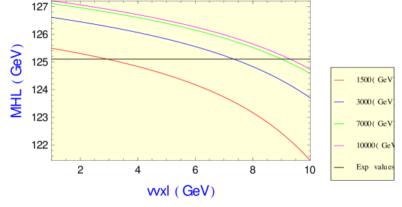
Figure 2: The masses of light scalars in terms of $v_{\chi^{\prime}}$ using the parameters defined at Eqs.(60,61).

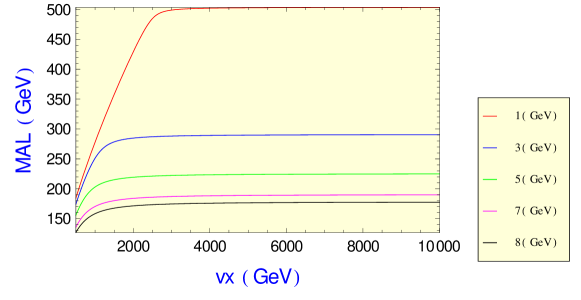
Figure 3: The masses of light pseudo-scalars in terms of $v_{\chi}$ using the parameters defined at Eqs.(60,61).

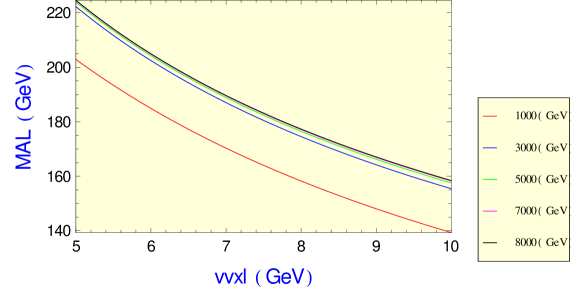
Figure 4: The masses of light pseudo-scalars in terms of $v_{\chi^{\prime}}$ using the parameters defined at Eqs.(60,61).

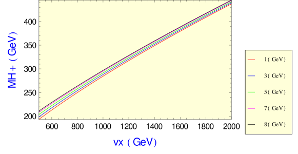
Figure 5: The masses of single scalars at first base, see Eq.(63), in terms of $v_{\chi}$ using the parameters defined at Eqs.(60,61).

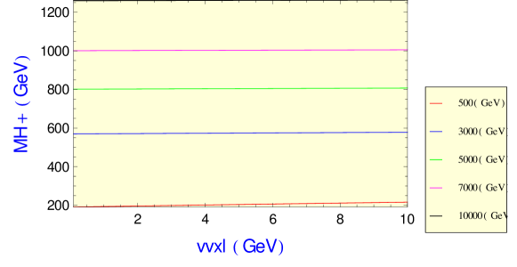
Figure 6: he masses of single scalars at second base, see Eq.(64), in terms of $v_{\chi^{\prime}}$ using the parameters defined at Eqs.(60,61).

Figure 7: The masses of single scalars at second base, see Eq.(64), in terms of $v_{\chi}$ using the parameters defined at Eqs.(60,61).

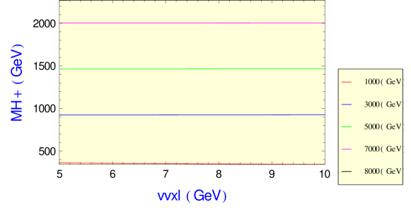
Figure 8: he masses of single scalars at base 2 in terms of $v_{\chi^{\prime}}$ using the parameters defined at Eqs.(60,61).

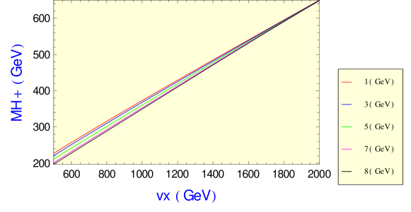
Figure 9: The masses of double scalars in terms of $v_{\chi}$ using the parameters defined at Eqs.(60,61).

Figure 10: he masses of double scalars in terms of $v_{\chi^{\prime}}$ using the parameters defined at Eqs.(60,61).

4 $R$-Parity charges at SUSY331RV

In the 3-3-1 model with heavy charged lepton [12] only the triplets are needed for generate masses for all the charged fermions.

However, if we want to allow neutrinos to get their masses and at the same time avoid the fast nucleon decay we can choose the following $R$-charges

$$n_{L} = n_{\eta}=n_{\eta^{\prime}}=n_{\rho}=n_{\rho^{\prime}}=-n_{\chi}=n_{\chi^{\prime}}=0,$$

$$n_{Q_{i}} = 1,\,\ n_{u}=n_{d_{i}}=n_{J_{i}}=-1.$$ (65)

In this case, the terms allow in our superpotential are

$$W = \mu_{0i}(\hat{L}_{aL}\hat{\eta}^{\prime})+\mu_{\eta}(\hat{\eta}\hat{\eta}^{\prime})+\mu_{\rho}(\hat{\rho}\hat{\rho}^{\prime})+\mu_{\chi}(\hat{\chi}\hat{\chi}^{\prime})+\lambda_{1abc}(\epsilon\hat{L}_{iL}\hat{L}_{jL}\hat{L}_{kL})+\lambda_{2ij}(\epsilon\hat{L}_{i}\hat{L}_{j}\hat{\eta})$$ (66)

$$+ \lambda_{3ij}(\hat{L}_{i}\hat{S}\hat{L}_{j})+\lambda_{4i}(\epsilon\hat{L}_{i}\hat{\chi}\hat{\rho})+f_{1}(\epsilon\hat{\rho}\hat{\chi}\hat{\eta})+f^{\prime}_{1}(\epsilon\hat{\rho}^{\prime}\hat{\chi}^{\prime}\hat{\eta}^{\prime})+\kappa_{1i}(\hat{Q}_{3}\hat{\eta}^{\prime})\hat{u}^{c}_{i}+\kappa_{2i}(\hat{Q}_{3}\hat{\rho}^{\prime})\hat{d}^{c}_{i}$$

$$+ \kappa_{3}(\hat{Q}_{3}\hat{\chi}^{\prime})\hat{J}^{c}+\kappa_{4\alpha i}(\hat{Q}_{\alpha}\hat{\eta})\hat{d}^{c}_{i}+\kappa_{5\alpha i}(\hat{Q}_{\alpha}\hat{\rho})\hat{u}^{c}_{i}+\kappa_{6\alpha\beta}(\hat{Q}_{\alpha}\hat{\chi})\hat{j}^{c}_{\beta}+\kappa_{7\alpha ij}(\hat{Q}_{\alpha}\hat{L}_{i})\hat{d}^{c}_{j}.$$

In our superpotential, we can generate mass to neutrinos without introduce the anti-sextet [24].

In the case non supersymmetric we have model with three triplets only if we introduce heavy charged lepton as done at [12].

4.1 The scalar potential at SUSY331RV

In the SUSY331RV there are $R$-violating interactions give the correct to neutrinos [24].

4.2 Numerical Analyses at SUSY331RV

We will use below the following set of parameters in the scalar potential:

$$f_{1}=1.43,\quad f^{\prime}_{1}=10^{-6},\quad{\rm(dimensionless)}$$ (67)

and

$$-k_{1}=k^{\prime}_{1}=10,\;-\mu_{\eta}=\mu_{\rho}=\mu_{\chi}=1000,\quad\mbox{(in GeV)},$$ (68)

we also use the constraint

$$V^{2}_{\eta}+V^{2}_{\rho}+2V^{2}_{2}=(246\;{\rm GeV})^{2}$$ (69)

coming from $M_{W}$, where, we have defined $V^{2}_{\eta}=v^{2}_{\eta}+v^{\prime 2}_{\eta}$ and $V^{2}_{\rho}=v^{2}_{\rho}+v^{\prime 2}_{\rho}$. Assuming that $v_{\eta}=20$, $v_{\chi}=1500$, $v^{\prime}_{\eta}=v^{\prime}_{\rho}=v^{\prime}_{\chi}=1$ in GeV, the value of $v_{\rho}$ is fixed by the constraint above.

With this set of values for the parameters the real mass eigenstates $H_{i}$ are (in GeV) $M_{H^{0}_{i}}=125.5,304.7,765.6,1818.2,2251.4,6620.3$, $i=1,\cdots,6$ and $M_{H_{j}}>M_{H_{i}}$ with $j>i$.

In the pseudoscalar sector we have verified analytically that the mass matrix, has two Goldstone bosons as it should. The other six physical pseudoscalars have the following masses, with the same parameters as before, in GeV, $M_{A_{i}}=304.4,765.6,2251.4,6620.3$.

In the Single charged Scalars we have two Goldstone bosons and nine massive states, in GeV. We get two unrelated bases. The first base is defined as $\eta^{-}_{1},\rho^{-},\eta^{\prime-}_{1},\rho^{\prime-}$ and we get the following masses $M_{H^{\pm}_{i}}=306.9,2252.1,6620.0$ The second base is defined as $\eta^{-}_{2},\chi^{-},\eta^{\prime-}_{2},\chi^{\prime-}$ and we get the following masses $M_{H^{\pm}_{i}}=298.8,908.5,6602.0$

In the Double charged Scalars we have one Goldstone bosons and seven massive states, in GeV, $M_{H^{\pm\pm}_{i}}=114.6,906.2,2195.2$.

We present next some plots to light scalar, first we fix some values for $v_{\chi^{\prime}}$ and present its mass in term of $v_{\chi}$, see Fig.(11). Next we fixed some values for $v_{\chi}$ and it is shown at Fig.(12).

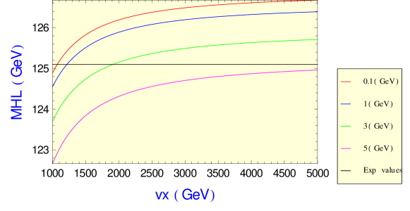
Figure 11: The masses of light scalars in terms of $v_{\chi}$ using the parameters defined at Eqs.(67,68).

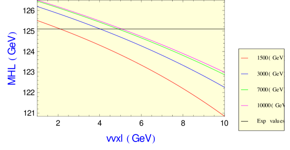
Figure 12: The masses of light scalars in terms of $v_{\chi^{\prime}}$ using the parameters defined at Eqs.(67,68).

5 Conclusions

We have studied the scalar potential of supersymmetric 3-3-1 model with the anti-sextet and without it and we show that our results are in agreement with the experimental contraints.

Acknowledgments

We would like thanks V. Pleitez, J. C. Montero and B. L. Schánchez-Vega for useful discussions above 3-3-1 models. We also to thanks IFT for the nice hospitality during my several visit to perform my studies about the severals 3-3-1 Models and also for done this article.

Appendix A Review Scalar Potential at m331

In the m331 the scalar sector is composed for the scalars defined at Eqs.(29 ,30). We can write the $SU(3)$ multiplets above in terms of the $SU(2)_{L}$ in the following way

$$\frac{Q^{SM}}{e} = \frac{1}{2}(\sigma_{3}+Y\,\ I_{2\times 2})=\frac{1}{2}\left(\begin{array}[]{ccc}1+Y&0\\ 0&Y-1\end{array}\right),$$ (72)

in the Standard Model the Higgs field has hypercharge (Y=+1), together with Eq.(72), it is given by

$$\Phi=\left(\begin{array}[]{c}h^{+}\\ h^{0}\end{array}\right)\sim({\bf 1},{\bf 2},+1).$$ (75)

Now we can decompose our Scalars fields in $SU(2)\otimes U(1)$ representations and the from group theory we can write [25]:

• ${\bf 3}_{0}\rightarrow{\bf 2}_{-1}\oplus{\bf 1}_{+2}$

  $$\eta = \left(\begin{array}[]{c}\Phi_{\eta}\\ \eta^{+}_{2}\end{array}\right)\sim({\bf 1},{\bf 3},0),$$ (78)

  $$\Phi_{\eta} = \left(\begin{array}[]{c}\eta^{0}\\ \eta^{-}_{1}\end{array}\right)\sim({\bf 1},{\bf 2},-1),\quad\eta^{+}_{2}\sim({\bf 1},{\bf 1},+2),$$ (81)

  where the singlet $\eta^{+}_{2}$ was introduced some years ago by Zee at [26]

• ${\bf 3}_{1}\rightarrow{\bf 2}_{1}\oplus{\bf 1}_{4}$

  $$\rho = \left(\begin{array}[]{c}\Phi_{\rho}\\ \rho^{++}\end{array}\right)\sim({\bf 1},{\bf 3},+1),$$ (84)

  $$\Phi_{\rho} = \left(\begin{array}[]{c}\rho^{+}\\ \rho^{0}\end{array}\right)\sim({\bf 1},{\bf 2},+1),\quad\rho^{++}\sim({\bf 1},{\bf 1},+4)$$ (87)

• ${\bf 3}_{-1}\rightarrow{\bf 2}_{-3}\oplus{\bf 1}_{0}$

  $$\chi = \left(\begin{array}[]{c}\Phi_{\chi}\\ \chi^{0}\end{array}\right)\sim({\bf 1},{\bf 3},-1),$$ (90)

  $$\Phi_{\chi} = \left(\begin{array}[]{c}\chi^{-}\\ \chi^{--}\end{array}\right)\sim({\bf 1},{\bf 2},-3),\quad\chi^{0}\sim({\bf 1},{\bf 1},0)$$ (93)

• ${\bf 6}_{0}\rightarrow{\bf 3}_{2}\oplus{\bf 2}_{-1}\oplus{\bf 1}_{-4}$

  $$S = \left(\begin{array}[]{cc}T&\frac{\Phi_{S}}{\sqrt{2}}\\ \frac{\Phi^{T}_{S}}{\sqrt{2}}&H^{--}_{2}\end{array}\right)\sim({\bf 1},{\bf 6}^{*},0),$$ (96)

  $$\Phi_{S} = \left(\begin{array}[]{c}h^{+}_{2}\\ \sigma^{0}_{2}\end{array}\right)\sim({\bf 1},{\bf 2},-1),\quad H^{--}_{2}\sim({\bf 1},{\bf 1},-4),$$ (99)

$\Phi_{S}$ is the Higgs doublet of the Standard Model, see Eq.(75), and the triplet

$$T = \left(\begin{array}[]{cc}\sigma^{0}_{1}&\frac{h^{+}_{1}}{\sqrt{2}}\\ \frac{h^{+}_{1}}{\sqrt{2}}&H^{--}_{1}\\ \end{array}\right)\sim({\bf 1},{\bf 3},+2),$$ (102)

was considered at [27].

Because of the anti-sextet, the scalar potential in the m331 become more complicated. The most general scalar potential involving triplets and the sextet is [25]

$$V(\eta,\rho,\chi,S) = V^{(2)}+V^{(3)}+V^{(4a)}+V^{(4b)}+V^{(4c)}+V^{(4d)}+V^{(4e)},$$ (103)

where

$$V^{(2)} = \mu_{1}^{2}(\eta^{\dagger}\eta)+\mu_{2}^{2}(\rho^{\dagger}\rho)+\mu_{3}^{2}(\chi^{\dagger}\chi)+\mu_{4}^{2}Tr[(S^{\dagger}S)],$$

$$V^{(3)} = \frac{f_{1}}{3!}\varepsilon_{ijk}\eta_{i}\rho_{j}\chi_{k}+f_{2}\rho_{i}\chi_{j}S^{\dagger ij}+f_{3}\eta_{i}\eta_{j}S^{\dagger ij}+\frac{f_{4}}{3!}\epsilon_{ijk}\epsilon_{lmn}S_{il}S_{jm}S_{kn}+H.c.,$$

$$V^{(4a)} = a_{1}(\eta^{\dagger}\eta)^{2}+a_{2}(\rho^{\dagger}\rho)^{2}+a_{3}(\chi^{\dagger}\chi)^{2}+(\chi^{\dagger}\chi)\left[a_{4}(\eta^{\dagger}\eta)+a_{5}(\rho^{\dagger}\rho)\right]+a_{6}(\eta^{\dagger}\eta)(\rho^{\dagger}\rho)$$

$$+ a_{7}(\chi^{\dagger}\eta)(\eta^{\dagger}\chi)+a_{8}(\chi^{\dagger}\rho)(\rho^{\dagger}\chi)+a_{9}(\eta^{\dagger}\rho)(\rho^{\dagger}\eta)+\left[a_{10}(\chi^{\dagger}\eta)(\rho^{\dagger}\eta)+H.c.\right],$$

$$V^{(4b)} = b_{1}(\chi^{\dagger}S)(\hat{\chi}\eta)+b_{2}(\rho^{\dagger}S)(\hat{\rho}\eta)+b_{3}(\eta^{\dagger}S)\left[(\hat{\chi}\rho)-(\hat{\rho}\chi)\right]+H.c.,$$

$$V^{(4c)} = c_{1}Tr[(\hat{\eta}S)(\hat{\eta}S)]+c_{2}Tr[(\hat{\rho}S)(\hat{\rho}S)]+H.c.,$$

$$V^{(4d)} = d_{1}(\chi^{\dagger}\chi)Tr[(S^{\dagger}S)]+d_{2}Tr[(\chi^{\dagger}S)(S^{\dagger}\chi)]+d_{3}(\eta^{\dagger}\eta)Tr[(S^{\dagger}S)]+d_{4}Tr[(\eta^{\dagger}S)(S^{\dagger}\eta)]$$

$$+ d_{5}(\rho^{\dagger}\rho)Tr[(S^{\dagger}S)]+d_{6}Tr[(\rho^{\dagger}S)(S^{\dagger}\rho)],$$

$$V^{(4e)} = e_{1}(Tr[(S^{\dagger}S)])^{2}+e_{2}Tr[(S^{\dagger}S)(S^{\dagger}S)],$$ (104)

and we have defined the $V^{(4b)}$ and $V^{(4c)}$ terms

$$\hat{x}_{ij}\equiv\epsilon_{ijk}x_{k},$$ (105)

with $x=\eta,\rho,\chi$. The constants $f_{i}$, $i=1,2,3$ and $4$ have dimension of mass.

	$\eta$	$\chi$	$\rho$	$S$
${\cal Z}_{7}$	$w^{3}$	$w^{6}$	$w^{5}$	$w^{4}$
${\cal Z}_{3}$	$w$	$1$	$w$	$w$

Table 1: Transformation properties of the scalar fields under ${\cal Z}_{7}\otimes{\cal Z}_{3}$, taken from [25].

In order to simplify the scalar potential, we impose the following discrete symmetry ${\cal Z}_{7}\otimes{\cal Z}_{3}$, defined at Tab.(1), which forbids the following coupling $a_{10},f_{3},f_{4},b_{1},b_{2},b_{3},c_{1}$ and $c_{2}$ in the scalar potential given at Eq.(104) as presented at [25].

The veves of our scalars are given at Eqs.(32). We will present in the following sub-sections the main results presented at [17].

We denote the $SU(3)_{L}$ gauge bosons by $V^{a}_{m}$ ($a=1,2,\ldots,8$) and since

$${\bf 8}_{0}\rightarrow{\bf 3}_{0}\oplus{\bf 2}_{3}\oplus{\bf 2}_{-3}\oplus{\bf 1}_{0},$$ (106)

we get a triplet, $V^{1}_{m},V^{2}_{m},V^{3}_{m}$, has hypercharge $0$, plus the doublet of bileptons, $\left(U^{++},V^{+}\right)$, its hypercharge is $Y=3$, and a singlet $V^{8}_{m}$ with $Y=0$.

A.1 CP-Even at MSUSY331

The square mass matrix coming from the base

$$\left(H_{\eta},H_{\rho},H_{\chi},H_{\sigma_{2}}\right)^{T}.$$ (107)

The mass spectrum and the eigenstates are get, see our Eq.(133), when we supose

$$|f_{1}|\sim w,\,\ |f_{2}|\sim w,$$ (108)

we obtain the following squares masases

$$m^{2}_{H^{0}_{1}} \approx -4\lambda(v^{2}+u^{2}+z^{2}),$$

$$m^{2}_{H^{0}_{2},H^{0}_{3}} \approx \frac{w^{2}}{4vuz}\left\{(su^{2}+rvz)w\pm\left[(su^{2}-rvz)^{2}w^{2}-\frac{4vu^{2}z}{w^{2}}\left[f_{1}f_{2}u^{2}-(f^{2}_{1}+f^{2}_{2})uz\right]\right]^{(1/2)}\right\},$$

$$m^{2}_{H^{0}_{4}} \approx -4\lambda_{3}w^{2},$$ (109)

where we are defining

$$r \equiv \frac{1}{w^{2}}(f_{1}v-wz)\approx-\frac{2}{uw}(\lambda_{5}v^{2}+\lambda_{6}u^{2}+2\lambda_{14}z^{2}),$$

$$s \equiv \frac{1}{w^{2}}(f_{1}z-vw).$$ (110)

This approximation implies

$$\lambda \equiv 4(2\lambda_{10}+\lambda_{11})\approx\lambda_{1}\approx\lambda_{2}\approx\lambda_{12}\approx\lambda_{13}\approx\frac{\lambda_{4}}{2}.$$ (111)

In this case the Standard Model Higgs Boson correspond to $H^{0}_{1}$, in the sense that its mass has no dependence in the $w$ parameter.

A.2 CP-Odd at MSUSY331

The square mass matrix coming from the base

$$\left(F_{\eta},F_{\rho},F_{\chi},F_{\sigma_{2}}\right)^{T},$$ (112)

the mass spectrum and the eigenstates are get, see our Eq.(133), to impose

$$f_{2}>0,$$ (113)

then the mass is given by:

$$m^{2}_{A^{0}_{1},A^{0}_{2}} \approx \frac{w^{2}}{4vuz}\left\{(su^{2}+rvz)w\pm\left[(su^{2}-rvz)^{2}w^{2}-\frac{4vu^{2}z}{w^{2}}\left[f_{1}f_{2}u^{2}-(f^{2}_{1}+-f^{2}_{2})uz\right]\right]^{(1/2)}\right\}.$$ (114)

A.3 Singly Charged at MSUSY331

The square mass matrix coming from the base

$$\left(\eta^{+}_{1},\rho^{+},\eta^{+}_{2},\chi^{+},h^{+}_{1},h^{+}_{2}\right)^{T}.$$ (115)

In this approximation two of the masses of the singly charged scalar are given

$$m^{2}_{H^{+}_{1},H^{+}_{2}} = m^{2}_{A^{0}_{1},A^{0}_{2}},$$

$$m^{2}_{H^{+}_{3},H^{+}_{4}} \approx f_{2}\frac{uw}{2z}.$$ (116)

A.4 Double Charged at MSUSY331

The square mass matrix coming from the base

$$\left(\rho^{++},\chi^{++},H^{+}_{1},H^{++}_{2}\right)^{T}.$$ (117)

The doubly charged scalar masses are

$$m^{2}_{H^{++}_{1},H^{++}_{2}} \approx \frac{w^{2}}{4z}\left\{u-2\lambda_{9}z\pm\left[(2\lambda_{9}z+u)^{2}+4z^{2}\right]^{(1/2)}\right\},$$

$$m^{2}_{H^{++}_{3},H^{++}_{4}} \approx f_{2}\frac{uw}{2z}.$$ (118)

Appendix B Construction Scalar Potential

To get the scalar potential of our model we have to eliminate the auxiliarly fields $F$ and $D$ that appear in our model. We are going to pick up the $F$ and $D$- terms we get

$${\cal L}^{Gauge}_{D} = \frac{1}{2}D^{a}D^{a}+\frac{1}{2}DD\,\ ,$$

$${\cal L}^{Scalar}_{F} = |F_{\eta}|^{2}+|F_{\rho}|^{2}+|F_{\chi}|^{2}+|F_{S}|^{2}+|F_{\eta^{\prime}}|^{2}+|F_{\rho^{\prime}}|^{2}+|F_{\chi^{\prime}}|^{2}+|F_{S^{\prime}}|^{2},$$

$${\cal L}^{Scalar}_{D} = \frac{g}{2}\left[\bar{\eta}\lambda^{a}\eta+\bar{\rho}\lambda^{a}\rho+\bar{\chi}\lambda^{a}\chi+\bar{S}\lambda^{a}S-\bar{\eta}^{\prime}\lambda^{*a}\eta^{\prime}-\bar{\rho}^{\prime}\lambda^{*a}\rho^{\prime}-\bar{\chi}^{\prime}\lambda^{*a}\chi^{\prime}-\bar{S}^{\prime}\lambda^{*a}S^{\prime}\right]D^{a}$$

$$+ \frac{g^{\prime}}{2}\left[\bar{\rho}\rho-\bar{\chi}\chi-\bar{\rho}^{\prime}\rho^{\prime}+\bar{\chi}^{\prime}\chi^{\prime}\right]D,$$

$${\cal L}^{W2}_{F} = \frac{1}{2}\left[\mu_{\eta}(\eta F_{\eta^{\prime}}+\eta^{\prime}F_{\eta}+\bar{\eta}\bar{F}_{\eta^{\prime}}+\bar{\eta^{\prime}}\bar{F}_{\eta})+\mu_{\rho}(\rho F_{\rho^{\prime}}+\rho^{\prime}F_{\rho}+\bar{\rho}\bar{F}_{\rho^{\prime}}+\bar{\rho^{\prime}}\bar{F}_{\rho})\right.$$

$$+ \left.\mu_{\chi}(\chi F_{\chi^{\prime}}+\chi^{\prime}F_{\chi}+\bar{\chi}\bar{F}_{\chi^{\prime}}+\bar{\chi^{\prime}}\bar{F}_{\chi})\right],$$

$${\cal L}^{W3}_{F} = |F_{\eta}|^{2}+|F_{\rho}|^{2}+|F_{\chi}|^{2}+|F_{S}|^{2}+|F_{\eta^{\prime}}|^{2}+|F_{\rho^{\prime}}|^{2}+|F_{\chi^{\prime}}|^{2}+|F_{S^{\prime}}|^{2}.$$

From the equation described above we can construct

$${\cal L}_{F} = {\cal L}^{Scalar}_{F}+{\cal L}^{W2}_{F}+{\cal L}^{W3}_{F}$$

$$= |F_{\eta}|^{2}+|F_{\rho}|^{2}+|F_{\chi}|^{2}+|F_{\eta^{\prime}}|^{2}+|F_{\rho^{\prime}}|^{2}+|F_{\chi^{\prime}}|^{2}$$

$$+ \frac{1}{2}\left[\mu_{\eta}(\eta F_{\eta^{\prime}}+\eta^{\prime}F_{\eta}+\bar{\eta}\bar{F}_{\eta^{\prime}}+\bar{\eta^{\prime}}\bar{F}_{\eta})+\mu_{\rho}(\rho F_{\rho^{\prime}}+\rho^{\prime}F_{\rho}+\bar{\rho}\bar{F}_{\rho^{\prime}}+\bar{\rho^{\prime}}\bar{F}_{\rho})\right.$$

$$+ \left.\mu_{\chi}(\chi F_{\chi^{\prime}}+\chi^{\prime}F_{\chi}+\bar{\chi}\bar{F}_{\chi^{\prime}}+\bar{\chi^{\prime}}\bar{F}_{\chi})\right]+\frac{1}{3}\left[f_{1}\epsilon(F_{\rho}\chi\eta+\rho F_{\chi}\eta+\rho\chi F_{\eta}\right.$$

$$+ \left.\bar{F}_{\rho}\bar{\chi}\bar{\eta}+\bar{\rho}\bar{F}_{\chi}\bar{\eta}+\bar{\rho}\bar{\chi}\bar{F}_{\eta})+f^{\prime}_{1}\epsilon(F_{\rho^{\prime}}\chi^{\prime}\eta^{\prime}+\rho^{\prime}F_{\chi^{\prime}}\eta^{\prime}+\rho^{\prime}\chi^{\prime}F_{\eta^{\prime}}\right.$$

$$+ \left.\bar{F}_{\rho^{\prime}}\bar{\chi^{\prime}}\bar{\eta^{\prime}}+\bar{\rho^{\prime}}\bar{F}_{\chi^{\prime}}\bar{\eta^{\prime}}+\bar{\rho^{\prime}}\bar{\chi^{\prime}}\bar{F}_{\eta^{\prime}})\right]\,\ ,$$

$${\cal L}_{D} = {\cal L}^{Gauge}_{D}+{\cal L}^{Scalar}_{D}$$ (120)

$$= \frac{1}{2}D^{a}D^{a}+\frac{1}{2}DD+\frac{g}{2}\left[\bar{\eta}\lambda^{a}\eta+\bar{\rho}\lambda^{a}\rho+\bar{\chi}\lambda^{a}\chi-\bar{\eta}^{\prime}\lambda^{*a}\eta^{\prime}-\bar{\rho}^{\prime}\lambda^{*a}\rho^{\prime}\right.$$

$$- \left.\bar{\chi}^{\prime}\lambda^{*a}\chi^{\prime}\right]D^{a}+\frac{g^{\prime}}{2}\left[\bar{\rho}\rho-\bar{\chi}\chi-\bar{\rho}^{\prime}\rho^{\prime}+\bar{\chi}^{\prime}\chi^{\prime}\right]D.$$

We will now show that these fields can be eliminated through the Euler-Lagrange equations

$$\frac{\partial{\cal L}}{\partial\phi}-\partial_{m}\frac{\partial{\cal L}}{\partial(\partial_{m}\phi)}=0\,\ ,$$ (121)

where $\phi=\eta,\rho,\chi,\eta^{\prime},\rho^{\prime},\chi^{\prime}$. Formally auxiliary fields are defined as fields having no kintetic terms. Thus, this definition immediately yields that the Euler-Lagrange equations for auxiliary fields simplify to $\frac{\partial{\cal L}}{\partial\phi}=0$.

$$V_{D} = -{\cal L}_{D}=\frac{1}{2}\left(D^{a}D^{a}+DD\right)$$ (122)

$$= \frac{g^{\prime 2}}{2}(\rho^{\dagger}\rho-\rho^{\prime\dagger}\rho^{\prime}-\chi^{\dagger}\chi+\chi^{\prime\dagger}\chi^{\prime})^{2}+\frac{g^{2}}{8}\sum_{i,j}\left(\eta^{\dagger}_{i}\lambda^{a}_{ij}\eta_{j}+\rho^{\dagger}_{i}\lambda^{a}_{ij}\rho_{j}+\chi^{\dagger}_{i}\lambda^{a}_{ij}\chi_{j}+S^{\dagger}_{ij}\lambda^{a}_{jk}S_{kl}\right.$$

$$- \left.\eta^{\prime\dagger}_{i}\lambda^{*a}_{ij}\eta^{\prime}_{j}-\rho^{\prime\dagger}_{i}\lambda^{*a}_{ij}\rho^{\prime}_{j}-\chi^{\prime\dagger}_{i}\lambda^{*a}_{ij}\chi^{\prime}_{j}-S^{\prime\dagger}_{ij}\lambda^{*a}_{jk}S^{\prime}_{kl}\right)^{2},$$

We can use the following relations

$$\lambda^{a}_{ij}\lambda^{a}_{kl}=\frac{(-2)}{3}\delta_{ij}\delta_{kl}+2\delta{il}\delta_{jk}.$$ (123)

Then

$$\eta^{\dagger}_{i}\eta_{j}\eta^{\dagger}_{k}\eta_{l}\lambda^{a}_{ij}\lambda^{a}_{kl}=-\frac{2}{3}\left(\eta^{\dagger}\eta\right)\left(\eta^{\dagger}\eta\right)+2\left(\eta^{\dagger}\eta\right)\left(\eta^{\dagger}\eta\right)=\frac{4}{3}\left(\eta^{\dagger}\eta\right)^{2},$$ (124)

in similar way

$$\rho^{\dagger}_{i}\rho_{j}\rho^{\dagger}_{k}\rho_{l}\lambda^{a}_{ij}\lambda^{a}_{kl} = \frac{4}{3}\left(\rho^{\dagger}\rho\right)^{2},$$

$$\chi^{\dagger}_{i}\chi_{j}\chi^{\dagger}_{k}\chi_{l}\lambda^{a}_{ij}\lambda^{a}_{kl} = \frac{4}{3}\left(\chi^{\dagger}\chi\right)^{2},$$

$$S^{\dagger}_{il}S_{mj}S^{\dagger}_{kn}S_{op}\lambda^{a}_{lm}\lambda^{a}_{no} = -\frac{2}{3}{\mbox{T}r}\left[\left(S^{\dagger}S\right)\left(S^{\dagger}S\right)\right]+2{\mbox{T}r}\left[(S^{\dagger}S)(S^{\dagger}S)\right].$$ (125)

By another hand

$$\eta^{\dagger}_{i}\eta_{j}\rho^{\dagger}_{k}\rho_{l}\lambda^{a}_{ij}\lambda^{a}_{kl} = -\frac{2}{3}\left(\eta^{\dagger}\eta\right)\left(\rho^{\dagger}\rho\right)+2\left(\rho^{\dagger}\eta\right)\left(\eta^{\dagger}\rho\right),$$

$$\eta^{\dagger}_{i}\eta_{j}\chi^{\dagger}_{k}\chi_{l}\lambda^{a}_{ij}\lambda^{a}_{kl} = -\frac{2}{3}\left(\eta^{\dagger}\eta\right)\left(\chi^{\dagger}\chi\right)+2\left(\chi^{\dagger}\eta\right)\left(\eta^{\dagger}\chi\right),$$

$$\rho^{\dagger}_{i}\rho_{j}\chi^{\dagger}_{k}\chi_{l}\lambda^{a}_{ij}\lambda^{a}_{kl} = -\frac{2}{3}\left(\rho^{\dagger}\rho\right)\left(\chi^{\dagger}\chi\right)+2\left(\chi^{\dagger}\rho\right)\left(\rho^{\dagger}\chi\right),$$ (126)

We can rewrite $V_{D}$ in the following way

$$V_{D} = \frac{g^{\prime 2}}{2}\left[(\rho^{\dagger}\rho)^{2}+(\chi^{\dagger}\chi)^{2}-2(\rho^{\dagger}\rho)(\chi^{\dagger}\chi)+\ldots\right]$$ (127)

$$+ \frac{g^{2}}{8}\left\{\frac{(-4)}{3}\left[(\eta^{\dagger}\eta)^{2}+(\rho^{\dagger}\rho)^{2}+(\chi^{\dagger}\chi)^{2}+(\eta^{\dagger}\eta)(\rho^{\dagger}\rho)+(\eta^{\dagger}\eta)(\chi^{\dagger}\chi)\right.\right.$$

$$+ \left.\left.(\eta^{\dagger}\eta)Tr[(S^{\dagger}S)]+(\rho^{\dagger}\rho)(\chi^{\dagger}\chi)+(\rho^{\dagger}\rho)Tr[(S^{\dagger}S)]+(\chi^{\dagger}\chi)Tr[(S^{\dagger}S)]\right]\right.$$

$$+ \left.4\left[(\eta^{\dagger}\rho)(\rho^{\dagger}\eta)+(\eta^{\dagger}\chi)(\chi^{\dagger}\eta)+Tr[(S^{\dagger}\eta)(\eta^{\dagger}S)]+(\rho^{\dagger}\chi)(\chi^{\dagger}\rho)\right.\right.$$

$$+ \left.\left.Tr[(S^{\dagger}\rho)(\rho^{\dagger}S)]+Tr[(S^{\dagger}\chi)(\chi^{\dagger}S)]\right]-\frac{2}{3}\left(Tr[(S^{\dagger}S)]\right)^{2}\right.$$

$$+ \left.2Tr[(S^{\dagger}S)(S^{\dagger}S)]+\ldots\right\}.$$

where $\ldots$ include the new fields due the SUSY algebra. As we want to compare our potential with the m331 we omitt those terms.

$$V_{F} = -{\cal L}_{F}=\sum_{m}F^{*}_{m}F_{m}$$

$$= \sum_{i,j,k}\left[\left|\frac{\mu_{\eta}}{2}\eta^{\prime}_{i}+\frac{f_{1}}{3}\epsilon_{ijk}\rho_{j}\chi_{k}+\frac{2f_{2}}{3}\eta_{i}S_{ij}\right|^{2}+\left|\frac{\mu_{\rho}}{2}\rho^{\prime}_{i}+\frac{f_{1}}{3}\epsilon_{ijk}\chi_{j}\eta_{k}+\frac{f_{3}}{3}\chi_{i}S_{ij}\right|^{2}\right.$$

$$+ \left.\left|\frac{\mu_{\chi}}{2}\chi^{\prime}_{i}+\frac{f_{1}}{3}\epsilon_{ijk}\rho_{j}\eta_{k}+\frac{f_{3}}{3}\rho_{i}S_{ij}\right|^{2}+\left|\frac{\mu_{s}}{2}S^{\prime}_{ij}+\frac{f_{2}}{3}\eta_{i}\eta_{j}+\frac{f_{3}}{3}\chi_{i}\rho_{j}\right|^{2}\right.$$

$$+ \left.\left|\frac{\mu_{\eta}}{2}\eta_{i}+\frac{f^{\prime}_{1}}{3}\epsilon_{ijk}\rho^{\prime}_{j}\chi^{\prime}_{k}+\frac{2f^{\prime}_{2}}{3}\eta^{\prime}_{i}S^{\prime}_{ij}\right|^{2}+\left|\frac{\mu_{\rho}}{2}\rho_{i}+\frac{f^{\prime}_{1}}{3}\epsilon_{ijk}\chi^{\prime}_{j}\eta^{\prime}_{k}+\frac{f^{\prime}_{3}}{3}\chi^{\prime}_{i}S^{\prime}_{ij}\right|^{2}\right.$$

$$+ \left.\left|\frac{\mu_{\chi}}{2}\chi_{i}+\frac{f^{\prime}_{1}}{3}\epsilon_{ijk}\rho^{\prime}_{j}\eta^{\prime}_{k}+\frac{f^{\prime}_{3}}{3}\rho^{\prime}_{i}S^{\prime}_{ij}\right|^{2}+\left|\frac{\mu_{s}}{2}S_{ij}+\frac{f^{\prime}_{2}}{3}\eta^{\prime}_{i}\eta^{\prime}_{j}+\frac{f^{\prime}_{3}}{3}\chi^{\prime}_{i}\rho^{\prime}_{j}\right|^{2}\right]$$

We can use the following relation

$$\epsilon_{ijk}\epsilon_{kmn}=\delta_{im}\delta_{jn}-\delta_{in}\delta_{jm}.$$ (129)

In both case $f_{3}=0=f^{\prime}_{3}$, then we get

$$\left|\frac{\mu_{\eta}}{2}\eta_{i}+\ldots\right|^{2} = \frac{\mu_{\eta}}{4}(\eta^{\dagger}\eta),\,\ \left|\frac{f_{1}}{3}\epsilon_{ijk}\rho_{j}\chi_{k}+\ldots\right|^{2}=\frac{f^{2}_{1}}{9}\left[(\rho^{\dagger}\rho)(\chi^{\dagger}\chi)-(\rho^{\dagger}\chi)(\chi^{\dagger}\rho)\right],$$

$$\left|\frac{\mu_{\rho}}{2}\rho_{i}+\ldots\right|^{2} = \frac{\mu^{2}_{\rho}}{4}(\rho^{\dagger}\rho),\,\ \left|\frac{\mu_{\chi}}{2}\chi_{i}+\ldots\right|^{2}=\frac{\mu^{2}_{\chi}}{4}(\chi^{\dagger}\chi),$$

$$\left|\frac{f_{1}}{3}\epsilon_{ijk}\chi_{j}\eta_{k}+\frac{f_{3}}{3}\chi_{i}S_{ij}+\ldots\right|^{2} = \frac{f^{2}_{1}}{9}\left[(\chi^{\dagger}\chi)(\eta^{\dagger}\eta)-(\chi^{\dagger}\eta)(\eta^{\dagger}\chi)\right]+\frac{f_{1}f_{2}}{9}\left[\epsilon(\chi^{\dagger}\eta^{\dagger})(\chi S)+H.c.\right]$$

$$+ \frac{f^{2}_{2}}{9}{\mbox{T}r}\left[(S^{\dagger}\chi)(\chi^{\dagger}S)\right],$$

$$\left|\frac{f_{1}}{3}\epsilon_{ijk}\rho_{j}\eta_{k}+\frac{f_{3}}{3}\rho_{i}S_{ij}+\ldots\right|^{2} = \frac{f^{2}_{1}}{9}\left[(\rho^{\dagger}\rho)(\eta^{\dagger}\eta)-(\rho^{\dagger}\eta)(\eta^{\dagger}\rho)\right]+\frac{f_{1}f_{2}}{9}\left[\epsilon(\rho^{\dagger}\eta^{\dagger})(\rho S)+H.c.\right]$$

$$+ \frac{f^{2}_{2}}{9}{\mbox{T}r}\left[(S^{\dagger}\rho)(\rho^{\dagger}S)\right],$$

$$\left|\frac{\mu_{s}}{2}S_{ij}+\ldots\right|^{2} = \frac{\mu^{2}_{s}}{4}(Tr[(S^{\dagger}S)])^{2},$$

$$\left|\frac{f_{1}}{3}\chi_{i}\rho_{j}+\ldots\right|^{2} = \frac{f^{2}_{1}}{9}\left[(\rho^{\dagger}\rho)(\chi^{\dagger}\chi)-(\rho^{\dagger}\chi)(\chi^{\dagger}\rho)\right].$$

Therefore

$$V_{F} = \frac{\mu^{2}_{\eta}}{4}(\eta^{\dagger}\eta)^{2}+\frac{\mu^{2}_{\rho}}{4}(\rho^{\dagger}\rho)^{2}+\frac{\mu^{2}_{\chi}}{4}(\chi^{\dagger}\chi)^{2}+\frac{\mu^{2}_{s}}{4}(Tr[(S^{\dagger}S)])^{2}$$ (131)

$$+ \frac{f^{2}_{1}}{9}\left[(\eta^{\dagger}\eta)(\rho^{\dagger}\rho)-(\rho^{\dagger}\eta)(\eta^{\dagger}\rho)+(\eta^{\dagger}\eta)(\chi^{\dagger}\chi)\right.$$

$$- \left.(\chi^{\dagger}\eta)(\eta^{\dagger}\chi)+(\rho^{\dagger}\rho)(\chi^{\dagger}\chi)-(\rho^{\dagger}\chi)(\chi^{\dagger}\rho)\right]+\frac{f^{2}_{2}}{9}\left\{Tr[(S^{\dagger}\rho)(\rho^{\dagger}S)]+Tr[(S^{\dagger}\chi)(\chi^{\dagger}S)]\right\}$$

$$+ \left\{\frac{f_{1}f_{2}}{9}\left[\epsilon(\rho^{\dagger}\eta^{\dagger})(\rho S)+\epsilon(\chi^{\dagger}\eta^{\dagger})(\chi S)\right]+H.c.\right\}+\ldots,$$

The scalar potential in this model is

$$V_{scalar} = m^{2}_{\eta}(\eta^{\dagger}\eta)+m^{2}_{\rho}(\rho^{\dagger}\rho)+m^{2}_{\chi}(\chi^{\dagger}\chi)+m^{2}_{S}Tr[(S^{\dagger}S)]-[k_{1}\epsilon\rho\chi\eta+k_{2}\chi\rho S^{\dagger}+H.c.]$$ (132)

$$+ \left(\frac{\mu^{2}_{\eta}}{4}-\frac{g^{2}}{6}\right)(\eta^{\dagger}\eta)^{2}+\left(\frac{\mu^{2}_{\rho}}{4}+\frac{g^{\prime 2}}{2}-\frac{g^{2}}{6}\right)(\rho^{\dagger}\rho)^{2}+\left(\frac{\mu^{2}_{\chi}}{4}+\frac{g^{\prime 2}}{2}-\frac{g^{2}}{6}\right)(\chi^{\dagger}\chi)^{2}$$

$$+ \left(\frac{f^{2}_{1}}{9}-\frac{g^{2}}{6}\right)(\eta^{\dagger}\eta)(\rho^{\dagger}\rho)+\left(\frac{f^{2}_{1}}{9}-\frac{g^{2}}{6}\right)(\eta^{\dagger}\eta)(\chi^{\dagger}\chi)+\left(\frac{f^{2}_{1}}{9}-g^{\prime 2}-\frac{g^{2}}{6}\right)(\rho^{\dagger}\rho)(\chi^{\dagger}\chi)$$

$$+ \left(\frac{g^{2}}{2}-\frac{f^{2}_{1}}{9}\right)(\eta^{\dagger}\rho)(\rho^{\dagger}\eta)+\left(\frac{g^{2}}{2}-\frac{f^{2}_{1}}{9}\right)(\eta^{\dagger}\chi)(\chi^{\dagger}\eta)+\left(\frac{g^{2}}{2}-\frac{f^{2}_{1}}{9}\right)(\rho^{\dagger}\chi)(\chi^{\dagger}\rho)$$

$$- \frac{g^{2}}{6}\left[(\eta^{\dagger}\eta)Tr[(S^{\dagger}S)]+(\rho^{\dagger}\rho)Tr[(S^{\dagger}S)]+(\chi^{\dagger}\chi)Tr[(S^{\dagger}S)]\right]$$

$$+ \frac{g^{2}}{2}Tr[(S^{\dagger}\eta)(\eta^{\dagger}S)]+\left(\frac{g^{2}}{2}+\frac{f^{2}_{2}}{9}\right)\left\{Tr[(S^{\dagger}\rho)(\rho^{\dagger}S)]+Tr[(S^{\dagger}\chi)(\chi^{\dagger}S)]\right\}$$

$$+ \left(\frac{\mu^{2}_{s}}{4}-\frac{g^{2}}{2}\right)\left(Tr[(S^{\dagger}S)]\right)^{2}+g^{2}Tr[(S^{\dagger}S)(S^{\dagger}S)]$$

$$+ \left\{\frac{f_{1}f_{2}}{9}\left[\epsilon(\rho^{\dagger}\eta^{\dagger})(\rho S)+\epsilon(\chi^{\dagger}\eta^{\dagger})(\chi S)\right]+H.c.\right\}+\ldots$$

and comparing it with Eq.(104) we can see

$$\mu^{2}_{1} = m^{2}_{\eta},\quad\mu^{2}_{2}=m^{2}_{\rho},\quad\mu^{2}_{3}=m^{2}_{\chi},\quad\mu^{2}_{4}=m^{2}_{S},$$

$$f_{1} = -3!k_{1},\quad f_{2}=-3!k_{2},$$

$$a_{1} = \frac{\mu^{2}_{\eta}}{4}-\frac{g^{2}}{6},\quad e_{1}=\frac{\mu^{2}_{s}}{4}-\frac{g^{2}}{2},\quad e_{2}=g^{2},$$

$$a_{2} = \frac{\mu^{2}_{\rho}}{4}+\frac{g^{\prime 2}}{2}-\frac{g^{2}}{6},a_{3}=\frac{\mu^{2}_{\chi}}{4}+\frac{g^{\prime 2}}{2}-\frac{g^{2}}{6},$$

$$a_{4} = -\frac{g^{2}}{6}+\frac{f^{2}_{1}}{9}=a_{6}=a_{7}=a_{8}=a_{9},$$

$$a_{5} = -g^{\prime 2}-\frac{g^{2}}{6}+\frac{f^{2}_{1}}{9},$$

$$d_{1} = -\frac{g^{2}}{6}=d_{3}=d_{4}=d_{5},$$

$$d_{2} = d_{4}=d_{6}=\frac{g^{2}}{2},$$

$$a_{10} = =0.$$ (133)

We get analytical two Goldstone bosons at CP-odd sector, two Goldstone bosons at Sngly charged sector and one Goldstone boson at Doubly charged sector. We will present our numerical rsults in Sec.(3.1).

References

- [1] M. Singer, J. W. F. Valle, and J. Schechter, Canonical neutral-current predictions from the weak-electromagnetic gauge group , Phys. Rev. D 22, 738, (1980).
- [2] F. Pisano and V. Pleitez, An model for electroweak interactions, Phys. Rev. D 46, 410, (1992); R. Foot, O. F. Hernandez, F. Pisano and V. Pleitez, Lepton masses in an gauge model, Phys. Rev. D 47, 4158, (1993).
- [3] R. Foot, H.N. Long and Tuan A. Tran, and gauge models with right-handed neutrinos, Phys. Rev. D 50, 34, (1994); J. C. Montero, F. Pisano and V. Pleitez, Phys. Rev. D 47, 2918, (1993); H.N. Long, model for right-handed neutrino neutral currents, Phys. Rev. D 54, 4691, (1996); H.N. Long, model with right-handed neutrinos, Phys. Rev. D 53, 437, (1996).
- [4] V. Pleitez, New fermions and a vector - like third generation in models, Phys. Rev.D53, 514, (1996).
- [5] T. V. Duong and E. Ma, Supersymmetric Gauge Model: Higgs Structure at the Electroweak Energy Scale, Phys. Lett.B316, 307 (1993).
- [6] H. N. Long and P. B. Pal, Nucleon instability in a supersymmetric model, Mod. Phys. Lett.A13, 2355, (1998).
- [7] J. C. Montero, V. Pleitez and M. C. Rodriguez, A Supersymmetric 3-3-1 model, Phys. Rev. D65, 035006, (2002).
- [8] M. Capdequi-Peyranère and M.C. Rodriguez, Charginos and neutralinos production at 3-3-1 supersymmetric model in e- e- scattering, Phys. Rev. D 65, 035001 (2002); M. C. Rodriguez, Double Chargino Production in scattering, Int. J. Mod. Phys. A 22, 6080, (2008).
- [9] J. C. Montero, V. Pleitez and M. C. Rodriguez, Supersymmetric 3-3-1 model with right-handed neutrinos, Phys. Rev. D 70, 075004, (2004).
- [10] D. T. Huong, M. C. Rodriguez and H. N. Long, Scalar sector of supersymmetric model with right-handed neutrinos, arXiv:hep-ph/0508045.
- [11] S. J. L. Rosner, Resource letter: The Standard model and beyond, Am. J. Phys. 71, 302, (2003); A. S. Kronfeld and C. Quigg, Resource Letter: Quantum Chromodynamics, Am. J. Phys.78, 1081, (2010).
- [12] V. Pleitez and M. D. Tonasse, Heavy charged leptons in an model, Phys. Rev. D 48, 2353, (1993).
- [13] J. C. Montero, V. Pleitez and O. Ravinez, Soft superweak CP violation in a model, Phys. Rev.D 60, 076003, (1999).
- [14] J. C. Montero, C. C. Nishi, V. Pleitez, O. Ravinez and M. C. Rodriguez, Soft CP violation in meson systems, Phys. Rev.D73, 016003, (2006).
- [15] M. C. Rodriguez, Scalar sector in the minimal supersymmetric 3-3-1 model, Int. J. Mod. Phys.A21, 4303, (2006).
- [16] V. Pleitez and M. D. Tonasse, Neutrinoless double beta decay in an SU(3)-L x U(1)-N model, Phys. Rev.D48, 5274, (1993), [arXiv:hep-ph/9302201 [hep-ph]].
- [17] M. D. Tonasse, The scalar sector of models, Phys. Lett.B381, 191, (1996).
- [18] R. A. Diaz, R. Martinez and F. Ochoa, The Scalar sector of the model, Phys. Rev.D69, 095009, (2004), [arXiv:hep-ph/0309280 [hep-ph]].
- [19] T. A. Nguyen, N. A. Ky and H. N. Long, The Higgs sector of the minimal 3 3 1 model revisited, Int. J. Mod. Phys.A15, 283, (2000), [arXiv:hep-ph/9810273 [hep-ph]].
- [20] Y. Giraldo and W. A. Ponce, Scalar Potential Without Cubic Term in 3-3-1 Models Without Exotic Electric Charges, Eur. Phys. J.C71, 1693 (2011), [arXiv:1107.3260 [hep-ph]].
- [21] A. E. Cárcamo Hernández, R. Martinez and J. Nisperuza, discrete group as a source of the quark mass and mixing pattern in models, Eur. Phys. J.C75, no.2, 72, (2015), [arXiv:1401.0937 [hep-ph]].
- [22] G. Aad et al. [ATLAS and CMS Collaborations], Combined Measurement of the Higgs Boson Mass in Collisions at and 8 TeV with the ATLAS and CMS Experiments, Phys. Rev. Lett.114, 191803, (2015), [arXiv:1503.07589 [hep-ex]].
- [23] M. C. Rodriguez, The Minimal Supersymmetric Standard Model (MSSM) and General Singlet Extensions of the MSSM (GSEMSSM), a short review, arXiv:1911.13043 [hep-ph].
- [24] J. C. Montero, V. Pleitez and M. C. Rodriguez, Lepton masses in a supersymmetric 3-3-1 model, Phys. Rev.D 65, 095008, (2002).
- [25] G. De Conto, A. C. B. Machado and V. Pleitez, Minimal 3-3-1 model with a spectator sextet, Phys. Rev. D92, 075031, (2015), [arXiv:1505.01343 [hep-ph]].
- [26] A. Zee, A Theory of Lepton Number Violation, Neutrino Majorana Mass, and Oscillation, Phys. Lett.B93, 389, (1980); [erratum: Phys. Lett.B95, 461, (1980)].
- [27] G. B. Gelmini and M. Roncadelli, Left-Handed Neutrino Mass Scale and Spontaneously Broken Lepton Number, Phys. Lett.B99, 411 (1981).
- [28] M. C. Rodriguez, Mass Spectrum in the Minimal Supersymmetric 3-3-1 model, J. Mod. Phys.2, 1193, (2011).