A Multiwavelength Study of ELAN Environments (AMUSE²). Mass budget, satellites spin alignment and gas infall in a massive $z\sim 3$ quasar host halo

Abstract

The systematic targeting of extended Ly$\alpha$ emission around high-redshift quasars resulted in the discovery of rare and bright Enormous Ly$\alpha$ Nebulae (ELANe) associated with multiple active galactic nuclei (AGN). We here initiate “a multiwavelength study of ELAN environments” (AMUSE²) focusing on the ELAN around the $z\sim 3$ quasar SDSS J1040+1020, a.k.a. the Fabulous ELAN. We report on VLT/HAWK-I, APEX/LABOCA, JCMT/SCUBA-2, SMA/850$\mu$m, ALMA/CO(5-4) and 2mm observations and compare them to previously published VLT/MUSE data. The continuum and line detections enable a first estimate of the star-formation rates, dust, stellar and molecular gas masses in four objects associated with the ELAN (three AGNs and one Ly$\alpha$ emitter), confirming that the quasar host is the most star-forming (SFR $\sim 500$ M_⊙ yr^-1) and massive galaxy ($M_{\rm star}\sim 10^{11}$ M_⊙) in the system, and thus can be assumed as central. All four embedded objects have similar molecular gas reservoirs ($M_{\rm H_{2}}\sim 10^{10}$ M_⊙), resulting in short depletion time scales. This fact together with the estimated total dark-matter halo mass, $M_{\rm DM}=(0.8-2)\times 10^{13}$ M_⊙, implies that this ELAN will evolve into a giant elliptical galaxy. Consistently, the constraint on the baryonic mass budget for the whole system indicates that the majority of baryons should reside in a massive warm-hot reservoir (up to $10^{12}$ M_⊙), needed to complete the baryons count. Additionally, we discuss signatures of gas infall on the compact objects as traced by Ly$\alpha$ radiative transfer effects and the evidence for the alignment between the satellites’ spins and their directions to the central.

1 Introduction

The discovery of bright and extended Ly$\alpha$ nebulae at high redshift, detected either around high-redshift radio galaxies (HzRGs; Miley & De Breuck 2008) or as so-called Lyman-Alpha blobs (LABs; e.g., Matsuda et al. 2004), pinpoints the rarest overdensity peaks in the early Universe (e.g., Steidel et al. 2000; Venemans et al. 2007; Yang et al. 2009, 2010; Bădescu et al. 2017). Indeed, HzRGs and LABs are extremely rare in the redshift range $2<z<5$, with number densities of a few times $10^{-8}$ Mpc^-3 (e.g., Willott et al. 2001; Venemans et al. 2007) and $\sim 10^{-6}-10^{-5}$ Mpc^-3 (e.g., Yang et al. 2009), respectively. At these locations, in the so-called protoclusters, the formation and evolution of the progenitors of present-day ellipticals can take place thanks to violent bursts of star formation and mergers of coeval galaxies (e.g., West 1994; Kauffmann 1996).

Recently, systematic surveys of radio-quiet quasars uncovered an additional population of rare Ly$\alpha$ nebulae with observed surface brightness SB${}_{\rm Ly\alpha}\gtrsim 10^{-17}$ erg s^-1 cm^-2 arcsec^-2 on $\gtrsim 100$ kpc, maximum extents of $>250$ kpc, and total Ly$\alpha$ luminosities of $L_{\rm Ly\alpha}>10^{44}$ erg s^-1 (Cantalupo et al. 2014; Hennawi et al. 2015; Cai et al. 2017; Arrigoni Battaia et al. 2018a, 2019). These enormous Ly$\alpha$ nebulae (ELANe; Cai et al. 2017) are therefore outliers with respect to known nebulosities associated with radio-quiet objects. The current statistics show that only $4^{+3}_{-2}\%$ of relatively bright quasars ($M_{i}<-24$ AB mag) are associated with ELANe. Converting the number density corresponding to the targeted quasars (e.g., Shen et al. 2020), this percentage translates to an ELAN number density of few times $10^{-6}$ Mpc^-3.

Interestingly, there are additional mounting lines of evidence suggesting that ELANe are located in overdense environments. Indeed, they are (i) all associated with multiple AGN, with up to four known quasars within the same structure (Hennawi et al. 2015), (ii) frequently associated with exceptional overdensities of Ly$\alpha$ emitters on small (Arrigoni Battaia et al. 2018a) and on large scales (Hennawi et al. 2015; Cai et al. 2017), and (iii) probably in fields characterized by high number counts of submillimeter sources (Arrigoni Battaia et al. 2018b). Despite these findings, a systematic study of the environment and nature of ELANe has not been conducted yet. For this reason, we initiated the project “a multiwavelength study of ELAN environments” (AMUSE²) collecting datasets from the rest-frame ultraviolet out to the submillimeter regime with the specific aim of studying their astrophysics, while firmly locating these large-scale structures in the wide framework of galaxy formation and evolution.

In this paper of the series, we focus on the $z=3.164$ ELAN discovered with the Multi Unit Spectroscopic Explorer (MUSE; Bacon et al. 2010) around the bright quasar SDSS J102009.99+104002.7 (hereafter QSO) by Arrigoni Battaia et al. (2018a), a.k.a. the Fabulous ELAN. The same work reported additional four objects embedded in the ELAN: a faint companion quasar (QSO2), a faint obscured (type-II) AGN (AGN1) and two Ly$\alpha$ emitters (LAE1 and LAE2). The ELAN shows a coherent velocity shear of $\sim 300$ km s^-1 across its whole extent ( $\sim 300$ projected kpc), which has been interpreted as the signature of inspiraling motions of accreting substructures within the bright quasar host halo (Arrigoni Battaia et al. 2018a).

Here we report on our extensive campaign targeting this ELAN with VLT/HAWK-I, APEX/LABOCA, JCMT/SCUBA-2, SMA, and ALMA. Specifically, our observations target the $H$-band, 870 $\mu$m (single-dish), 850 $\mu$m (single-dish), 450 $\mu$m (single-dish), 850 $\mu$m (interferometer), 2 mm and the CO(5-4) rotational transition of the carbon monoxide, respectively.

The paper is structured as follows. In section 2 we report on our observations and data reduction for each individual instrument/dataset. Section 3 presents the observational results, quantifying the significance of the detections. The observational results allowed us to examine several aspects of the nature and astrophysics of this ELAN. In section 4, we first estimate the star formation, dust, stellar and molecular gas masses, and infer the dark matter halo mass with two orthogonal methods. In this way, we obtain a first-order mass budget of the whole system (section 4.4), which we use to forecast its evolution (section 4.5). We discuss in section 5 the evidence of alignment of the satellite spins with respect to their positional vector to the central quasar in the framework of the tidal torque theory. Section 6 then presents a comparison of the rotational transition CO(5-4) detected at the location of compact objects with the resonant Ly$\alpha$ line in their vicinity, discussing possible signatures of infall. Next, sections 7 and 8 briefly discuss the powering of the ELAN and the constraints on extended molecular gas, respectively. Finally, we summarize our findings in section 9.

Throughout this paper, we adopt the cosmological parameters $H_{0}=70$ km s^-1 Mpc^-1, $\Omega_{\rm M}=0.3$, and $\Omega_{\Lambda}=0.7$. In this cosmology, $1\arcsec$ corresponds to about 7.6 physical kpc at $z=3.164$ (redshift of the ELAN and the bright quasar from Arrigoni Battaia et al. 2018a). All distances reported in this work are proper.

2 Observations and data reduction

2.1 APEX/LABOCA

We used the Large APEX BOlometer CAmera (LABOCA; Siringo et al. 2009) on the APEX telescope to map a field of $\sim 68$ arcmin² around the ELAN hosting QSO. The 295 bolometers of LABOCA operate at an effective frequency of 345 GHz (or a wavelength of 870 $\mu$m), and the instrument is characterized by a main beam of 19$\arcsec$. The observations were conducted in service mode in October 2016 (ID: 098.A-0828(B); PI: F. Arrigoni Battaia) with zenith opacities between 0.2 and 0.4 at 870 $\mu$m. The field has been covered with a raster of spiral scanning mode, which optimizes the sampling of the field-of-view with the LABOCA instrument. The total integration time on source resulted in 22 hours consisting of 176 scans of 7.5 minutes each. The observations have been acquired with regular standard calibrations for pointing, focus and flux calibration (see e.g. Siringo et al. 2009 for details).

The data reduction was performed with the Python-based BOlometer data Analysis Software package (BoA; Schuller 2012) following the steps indicated in Siringo et al. (2009) and Schuller et al. (2009). Specifically, BoA processes LABOCA data including flux calibration, opacity correction, noise removal, and despiking of the timestreams. We ran BoA using the default reduction script reduce-map-weaksource.boa which also filters out the low-frequency noise below 0.3 Hz. The scans are then co-added after being variance-weighted. The final outputs are a beam-smoothed flux density and a noise maps. The final map achieves a root-mean-square (rms) noise level of $2.6-3$ mJy beam^-1 in its central part. We show the map for the full area covered in Appendix A.

2.2 JCMT/SCUBA-2

The SCUBA-2 observations for this ELAN field were conducted at JCMT during flexible observing in 2018 February 12, and March 29 (program ID: M18AP054; PI: M. Fumagalli) under good weather conditions (band 1 and 2, $\tau_{225{\rm GHz}}\leq 0.07$). The SCUBA-2 instrument observes simultaneously the same field at 850 and 450 $\mu$m, with an effective beam FWHM of $14.6\arcsec$ and $9.8\arcsec$, respectively (Dempsey et al. 2013). The observations were performed with a Daisy pattern covering $\simeq 13.7\arcmin$ in diameter, and were centered at the location of QSO (and thus the ELAN). To facilitate the scheduling we divided the observations in 5 scans/cycles of about 30 minutes, for a total of 2.5 hours.

For the data reduction we closely followed the procedures in Chen et al. (2013a) and Arrigoni Battaia et al. (2018b). In brief, we reduced the data using the Dynamic Iterative Map Maker (DIMM) included in the Sub-Millimetre User Reduction Facility (SMURF) package from the STARLINK software (Jenness et al. 2011; Chapin et al. 2013). We adopted the standard configuration file dimmconfig_blank_field.lis for our science purposes. We thus reduced each scan and the MOSAIC_JCMT_IMAGES recipe in PICARD, the Pipeline for Combining and Analyzing Reduced Data (Jenness et al. 2008), was used to coadd the reduced scans into the final maps.

We applied to these final maps a standard matched filter to increase the point source detectability, using the PICARD recipe SCUBA2_MATCHED_FILTER. We adopted the standard flux conversion factors (FCFs; 491 Jy pW^-1 for 450 $\mu$m and 537 Jy pW^-1 for 850 $\mu$m) with 10% upward corrections for flux calibration. The relative calibration accuracy is shown to be stable and good to 10% at 450 $\mu$m and 5% at 850 $\mu$m (Dempsey et al. 2013).

The final noise level at the location of the ELAN for our data is 1.01 mJy beam^-1 and 10.97 mJy beam^-1 at 850 $\mu$m and 450 $\mu$m, respectively. Appendix A presents the SCUBA-2 maps for the whole field-of-view covered. In the reminder of this work we focus only on the ELAN location.

2.3 SMA

We performed the SMA (Ho et al., 2004) observations of this ELAN (Project code: 2017A-S015, PI: F. Arrigoni Battaia) on June 21 (UTC 3:00-8:30), June 27 (UTC 3:00-7:30), and July 10 (UTC 3:30-6:30) of 2017, in the compact array configuration. However, for the observations on June 27, we only utilized the data taken after UTC 6:30 because we noticed a large antenna pointing error before then. The atmospheric opacity at 225 GHz ($\tau_{\mbox{\tiny 225 GHz}}$) were 0.1-0.15, $\sim$0.1, and $\sim$0.05 during these three tracks of observations.

The observations were carried out in dual receiver mode by tuning the 345 GHz and 400 GHz receivers to the same observing frequencies. These two receivers took left and right circular polarization, respectively, and covered the observing frequency 329-337 GHz in the lower sideband and 345-353 GHz in the upper sideband. Correlations were performed by the SMA Wideband Astronomical ROACH2 Machine (SWARM) which sampled individual sidebands with 16384$\times$4 spectral channels. The integration time was 30 seconds. Prior to data calibration, we binned every 16 spectral channels to reduce filesizes. The observations on our target source cover the uv distance range of $\sim$8.5-88.5 $k\lambda$.

The target sources were observed in scans of 12 minute duration, which were bracketed by scans on the gain calibration quasar source 1058+015 with 3 minutes duration. We observed Titan in the first two tracks, and observed Callisto in the last track for absolute flux calibrations. We follow the standard data calibration strategy of SMA. The application of Tsys information and the absolute flux, passband, and gain calibrations were carried out using the MIR IDL software package (Qi, 2003). The absolute flux scalings were derived by comparing the visibility amplitudes of the gain calibrators with those of the absolute flux calibrators (i.e., Titan and Callisto). The derived and applied fluxes of 1058+015 were 2.5 Jy in the first two tracks, and 2.7 Jy in the last track. We nominally quote the $\sim$15% typical absolute flux calibration error of SMA.

After calibration, the zeroth-order fitting of continuum levels and the joint weighted imaging of all continuum data were performed using the Miriad software package (Sault et al., 1995). We performed zeroth-order multi-frequency imaging combining the upper- and lower-sideband data, to produce a sensitive continuum image at the central observing frequency (i.e., the local oscillator frequency). Due to the different performance of the 345 GHz and 400 GHz receivers at the same observing frequency, it would be incorrect to treat half of the difference of the parallel hand correlations (i.e., $(LL-RR)/2$) as the thermal noise map. Instead, we constructed the approximated noise map by first smoothing the upper-sideband image to the angular resolution of that of the lower-sideband image, and then take half of their difference. Using natural weighting, we obtained a $\theta_{\mbox{\tiny maj}}$ $\times$ $\theta_{\mbox{\tiny min}}$ $=$ 2$\farcs$4 $\times$ 2$\farcs$0 (P.A.=67^∘) synthesized beam, and a rms noise level of 1.4 mJy beam^-1.

2.4 ALMA

We performed four epochs of ALMA observations towards this ELAN (Project code: 2017.1.00560.S, PI: F. Arrigoni Battaia), on March 23, 24, 26, and 27 (UTC) of 2018 to constrain the CO(5-4) line emission ($\nu_{\rm rest}=576.267$ GHz) and its underlying $2$ mm continuum. The pointing and phase referencing center is R.A. (J2000) = 10${}^{\mbox{\tiny h}}$20${}^{\mbox{\tiny m}}$09${}^{\mbox{\tiny s}}$.42, and Decl. (J2000) = 10^∘40^′08^′′.71. Combining all existing data yields an overall uv distance range covered of 12-740 meters.

The spectral setup of all our observations is identical. There were two 2 GHz wide spectral windows (channel spacing 15.625 MHz) centered at the sky frequencies 149.514 GHz and 151.201 GHz, and two 1.875 GHz wide spectral windows (channel spacing 3.906 MHz) centered at the sky frequencies 137.784 GHz and 139.472 GHz. The latter two spectral windows with channel width of about 8.5 km s^-1 are expected to encompass the CO(5-4) emission.

For all four epochs of observations, the quasar J1058+0133 was chosen as the flux and passband calibrator. We assume that J1058+0133 has a 3.09 Jy absolute flux and -0.46 spectral index at the reference frequency 144.493 GHz, which was based on interpolating the calibrator grid survey measurements taken in Band 3 ($\sim$91 and 103 GHz) on March 25, 2018, and in Band 7 ($\sim$343 GHz) on February 09, 2018. Based on the results of the calibrator grid survey, we expect a nominal $\sim$10% absolute flux error, and $\sim$0.1 in-band spectral index error as the grid survey measurements are sparsely sampled in time. We observed the quasar J1025+1253 approximately every 11 minutes for complex gain calibration.

We calibrated the data using the CASA software package (McMullin et al., 2007) version 5.1. The derived fluxes of the gain calibrator J1025+1253 were in the range $0.42-0.48$ Jy. We fit the continuum baselines using the CASA task uvcontsub. We jointly imaged all continuum data using the CASA task clean, which produced the Stokes I image by averaging the parallel linear correlation data (i.e., I = $(XX+YY)/2$). Our target sources are presumably weakly or not polarized. Therefore, we regarded the $(XX-YY)/2$ image as an approximated thermal noise map. The Briggs Robust = 2 weighted image achieved a synthesized beam of $\theta_{\mbox{\tiny maj}}\times\theta_{\mbox{\tiny min}}$= 0$\farcs$95$\times$0$\farcs$94 (P.A.=-5.3^∘), and a rms noise of 4.7 $\mu$Jy beam^-1.

For the spectral windows including the CO(5-4) emission, we generate the continuum from the channels not affected by line emission as identified from the datacubes, and subtract it from the data. Continuum-subtracted datacubes were created with the CASA task tclean, using Briggs cleaning with robustness parameter of 2 (corresponding to natural visibility weights). This approach maximises the signal-to-noise ratio and it is frequently used in observations of high-z quasars (e.g., Decarli et al. 2018; Bischetti et al. 2021).

2.5 VLT/HAWK-I

We observed in $H$-band the ELAN around QSO with the wide-field near-infrared imager HAWK-I (Casali et al. 2006) on the Unit Telescope 4 (UT4, Yepun) of the Very Large Telescope (VLT) in service mode under the project 0102.C-0589(D) (PI: F. Vogt). In this work we only focus on the $H$-band observations acquired with clear weather, i.e. 15, 23 February; 9, 22, 23 March 2019. HAWK-I has a field of view of $7\arcmin.5\times 7\arcmin.5$ covered by an array of $2\times 2$ Hawaii-2RG detectors separated by $15\arcsec$ gaps. The observational strategy consisted in three fast 60s $H$-band exposures per observing block (OB) to which it is applied a dithering within a jitter box of 15$\arcsec$. The ELAN system was always acquired in the fourth quadrant, Q4, of the detector array. The total on-source time for our clear weather observations consists of 12 OBs, i.e. 36 minutes on source for the $H$-band.

We reduced the data with the standard ESO pipeline version 2.4.3 for HAWK-I. In brief, the data are corrected for dark current and are flat-fielded. The sky subtraction is performed using the algorithm pawsky$\_$mask, which iteratively estimates the background by stacking with rejection the science frames and by constructing a mask for the objects in the data. The sky estimation ends once the number of masked pixels converges. The photometry of the images is calibrated with 2MASS stars in the field of view of our observations, achieving a $1\sigma$ AB magnitude limit of 26.0 mag in 1 arcsec² aperture. The intrinsic uncertainty on the photometric calibration is 0.1 mag. The astrometry is calibrated against the 2MASS catalogue (about 20 stars), with an average error in the coordinates fit of $\sim 0.2\arcsec$. This astrometry calibration agrees well with the GAIA DR2 catalogue (Gaia Collaboration et al. 2018). The seeing in the final combined image is of $0.5\arcsec$.

3 Results

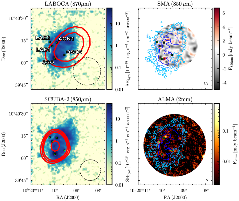
Figure 1: Top left: The detection obtained with LABOCA (red contours) is compared to the ELAN discovered in Ly$\alpha$ with MUSE (color map). The red contours indicate the isophotes at S/N=3, and 4. The dashed circle indicates the beam of LABOCA (FWHM=19$\arcsec$). Bottom left: Same as the top left panel, but for the central detection for the SCUBA-2 instrument at 850 $\mu$m. The red contours indicate the isophotes at S/N=3, 4, 5, and 10. The dashed circle indicates the beam of SCUBA-2 at 850 $\mu$m (FWHM=14$\arcsec$). Top right: Continuum map at $\sim 850$ $\mu$m obtained with SMA (HPBW$\sim 25\arcsec$). For comparison, the blue to turquoise contours indicate S/N = 2, 10, and 40 for the ELAN as detected with MUSE (Arrigoni Battaia et al. 2018a). Five sources are detected in this map (see Section 3.2 and Figure 2). Bottom right: Same as top right panel, but at $2$ mm using all the ALMA data (HPBW$=42.257\arcsec$). Eight sources are detected in this map (see Section 3.3 and Figure 3).

3.1 Single dish continuum detections

The first data we acquired on this system, the 870 $\mu$m APEX/LABOCA data, revealed a 4.8$\sigma$ detection of ${12.5\pm 2.6}$ mJy at the position of the ELAN (see top-left panel in Figure 1). This surprisingly strong detection in an ELAN was then confirmed by the deeper 850 $\mu$m JCMT/SCUBA-2 observations, with a flux density of ${12.7\pm 1.0}$ mJy (see bottom-left panel in Figure 1). We corrected this observed flux densities for flux boosting (see appendix B), obtaining f${}_{\rm Deboosted}=10.5\pm 2.2$, and $11.7\pm 0.9$ mJy, respectively for the LABOCA and SCUBA-2 detections (Table LABEL:tab:SingleDish).

Given the radio-quietness of all the sources embedded within the ELAN (Arrigoni Battaia et al. 2018a), the detected emission traces thermal dust emission from embedded starbusting galaxies. The strong detected fluxes would imply a star-formation rate of SFR$=1680\pm 338$ M_⊙ yr^-1, following Cowie et al. (2017). These unexpectedly bright single-dish detections have been a fundamental stepping stone for the follow-up observations with interferometers.

The SCUBA-2 450 $\mu$m data are not deep enough to detect emission from the ELAN. We report the 450 $\mu$m upper limit at the location of the 850 $\mu$m detection in Table LABEL:tab:SingleDish.

Table 1: The continuum detections from LABOCA and SCUBA2.

ID	f	SNR	fDeboosted
	(mJy)		(mJy)
LABOCA(870$\mu$m)	12.5	4.8	10.5$\pm 2.2$
SCUBA2(850$\mu$m)	12.7	12.6	11.7$\pm 0.9$
SCUBA2(450$\mu$m)	$<33^{a}$	-	-

3.2 SMA continuum at 850 $\mu$m

We extracted continuum sources from the SMA continuum map (top right panel in Figure 1) using the same algorithm described in e.g., Arrigoni Battaia et al. (2018b), but working with the SMA beam of the current dataset. Briefly, the algorithm iteratively searches for maxima in the S/N map (Figure 2) while subtracting (at their locations) mock sources normalized to those peaks. The iterations are stopped once S/N$=2$ is reached. The S/N peaks found by the algorithm are included in a source candidate catalog. In the current case, the algorithm found 7 sources. Subsequently, the same algorithm is applied to the negative dataset down to the same S/N threshold to estimate the number of spurious sources and clean the aforementioned catalog. We find no spurious sources within a radius of $R=7\arcsec$ from the center of the map, one such source in the annuli within $7\arcsec<R<10.5\arcsec$, and four for $R>10.5\arcsec$. Therefore, we consider reliable five of the seven sources detected in our map (yellow diamonds in Figure 2). The two potentially spurious sources are indicated with cyan diamonds in Figure 2, and are located respectively in the $7\arcsec<R<10.5\arcsec$ and $R>10.5\arcsec$ regions. This analysis is confirmed by the absence of emission at these two locations in the ALMA continuum map (see section 3.3), while all the other sources are very close to the positions of known sources associated with the ELAN or with ALMA detections (see section 3.3). The detected sources are QSO, QSO2, AGN1, LAE1, and a newly discovered source SMG1. The positions, S/N and fluxes for the five detections are listed in Table LABEL:tab:Interf, together with the deboosted fluxes estimated as explained in Appendix C. Summing up the deboosted fluxes of all detected sources, we find agreement within uncertainties with the detections in the single-dish datasets, $14.7\pm 2.8$ mJy. Therefore, all the continuum emission detected by LABOCA and SCUBA-2 is ascribed to compact sources.

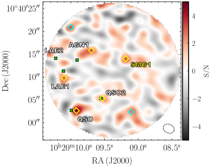
Figure 2: S/N map at $\sim 850$ $\mu$m obtained with SMA. We show the location of (i) the detections down to S/N=2 (yellow diamonds), (ii) the spurious sources (cyan diamonds), and (iii) the location of known sources associated with the ELAN (green crosses; Arrigoni Battaia et al. 2018a). A newly discovered source is named SMG1. The beam of the observations is indicated in the bottom-right corner.

Table 2: The continuum measurements from ALMA, SMA, HAWK-I and MUSE.

ID	fALMA	SNR	f${}_{\rm ALMA}^{\rm Deboosted}$	R.A.	Dec	fSMA	SNR	f${}_{\rm SMA}^{\rm Deboosted}$	$H$	$i$	$r$
	(mJy)		(mJy)	(J2000)	(J2000)	(mJy)		(mJy)	(AB)	(AB)	(AB)
QSO	0.24	34.6	0.23$\pm$0.01	10:20:10.00	+10:40:02.7	6.8b	4.9	5.7$\pm$1.8	17.1$\pm$0.1	17.98$\pm$0.01	17.67$\pm$0.01
QSO2	0.06	8.9	0.06$\pm$0.01	10:20:09.56	+10:40:05.3	3.3b	2.4	2.0$\pm$1.0	23.5$\pm$0.1	24.30$\pm$0.02	24.10$\pm$0.01
LAE1	0.17	23.9	0.17$\pm$0.01	10:20:10.15	+10:40:10.6	3.6b	2.6	2.4$\pm$1.1	24.6$\pm$0.6	25.43$\pm$0.05	25.32$\pm$0.05
LAE2	$<0.01^{\rm a}$	-	-	-	-	$<2.8^{\rm a}$	-	-	$>$26.8d	$>$28.6d	$>$28.6d
AGN1	0.19	18.2	0.13$\pm$0.01	10:20:09.83	+10:40:14.7	4.0b	2.8	2.8$\pm$1.2	24.7$\pm$0.7	26.20$\pm$0.20	26.30$\pm$0.20
SMG1	0.03	4.4	0.02$\pm$0.01	10:20:09.18	+10:40:13.4	3.1b	2.2	1.8$\pm$0.9	24.6$\pm$0.3	26.14$\pm$0.12	26.88$\pm$0.23
S1	0.04	6.6	0.04$\pm$0.01	10:20:09.41	+10:40:04.9	$<2.8^{\rm c}$	-	-	24.8$\pm$0.3	27.18$\pm$0.31	$>$28.6d
S2	0.03	4.1	0.03$\pm$0.01	10:20:10.16	+10:40:08.6	$<2.8^{\rm c}$	-	-	23.2$\pm$0.1	24.77$\pm$0.03	24.75$\pm$0.03
S3	0.03	4.1	0.03$\pm$0.01	10:20:08.78	+10:40:16.3	$<2.8^{\rm c}$	-	-	$>$26.8d	$>$28.6d	$>$28.6d

3.3 ALMA continuum at 2 mm

We extracted sources from the ALMA continuum map at 2 mm (bottom right panel in Figure 1) following the same method as for the SMA data, but using the ALMA beam. We considered as reliable only sources with S/N$>3.7$. Indeed, above this threshold we did not find any spurious source in the negative map. Using this threshold, we found eight detections, shown as black circles in Figure 3: (i) the known sources QSO, QSO2, LAE1, and AGN1, (ii) the source SMG1 discovered with SMA, and (iii) three additional sources which we dubbed S1, S2, and S3. The coordinates, fluxes and S/N of all the sources, as well as their deboosted fluxes estimated as explained in Appendix D are listed in Table LABEL:tab:Interf.

As evident from Figure 3, some of the ALMA detections have shifts of $\sim$ few arcseconds with respect to the Ly$\alpha$ locations and to the SMA locations. While the latter is likely due to the low SNR of the SMA detections, we discuss in detail the shifts with respect to the Ly$\alpha$ locations in section 6.

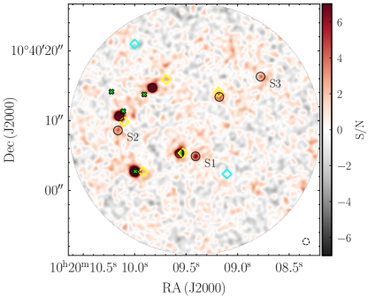
Figure 3: S/N map at $\sim 2$ mm obtained with ALMA. We show the location of (i) the detections for S/N$>3.7$ (see section 3.3 for details), (ii) the SMA detections (yellow diamonds), (iii) the spurious SMA sources (cyan diamonds), and (iv) the location of known sources associated with the ELAN (green crosses; Arrigoni Battaia et al. 2018a). Three newly discovered sources are named S1, S2, and S3. The beam of the observations is indicated in the bottom-right corner.

3.4 HAWK-I and VLT/MUSE counterparts

We inspected the $H$-band HAWK-I data presented in section 2.5 at the location of the sources so far discussed. As can be seen in Figure 4, we find clear detections for QSO, QSO2, S2, SMG1, and AGN1, while fainter emission at the location of LAE1 and S1. LAE2 and S3 are undetected at the current depth. We extract magnitudes with apertures of 2$\arcsec$ diameter ($4\times$ the seeing) for all the sources except QSO. Indeed, its flux is better captured by a 3$\arcsec$ diameter aperture. We list the derived magnitudes in Table LABEL:tab:Interf.

Further, we obtained the observed optical magnitude, $i$ and $r$, of all sources within the aforementioned apertures from the MUSE data presented in Arrigoni Battaia et al. (2018a). These magnitudes are listed in Table LABEL:tab:Interf. We note that the MUSE $i$-band magnitude for AGN1 is different from the magnitude listed in Arrigoni Battaia et al. (2018a) because in that study the authors rely on the compact Ly$\alpha$ emission for determining the source position. However, there is an important shift between Ly$\alpha$ and the near and far-infrared continua detected in this work (Figure 4; see discussion in section 6).

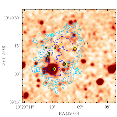
Figure 4: $H$-band HAWK-I data within the field of view of Fig. 1 smoothed with a 1$\arcsec$ Gaussian kernel. We highlight the location of (i) the ALMA detections (black circles), (ii) the SMA detections (yellow diamonds), (iii) the spurious SMA sources (cyan diamonds), and (iv) the location of known sources associated with the ELAN (green crosses; Arrigoni Battaia et al. 2018a). The ELAN isophotes are indicated as in Figure 1.

3.5 ALMA CO(5-4) line detections

We rely on the publicly available code LineSeeker (González-López et al. 2017) to robustly identify sources with CO(5-4) line emission in the ALMA observations. Indeed LineSeeker has been developed to systematically search for line emissions in ALMA data and quantify their significance (e.g., González-López et al. 2019). The code looks for signal in the ALMA datacubes on a channel by channel basis after convolving the data along the spectral axis with Gaussian kernels of different spectral widths. A list of line candidates is obtained by joining detected signal on different channels using the DBSCAN algorithm (Ester et al. 1996). LineSeeker finally provides a S/N for each emission line candidate. This S/N is defined as the maximum value obtained from the different convolutions. Further, it runs the search algorithm also on the negative datacube and on simulated cubes to estimate the significance of the line candidates S/N, providing probabilities of the line being false.

Here we focus on 100$\%$ fidelity sources, i.e., sources whose probability of being false is 0 and whose S/N is larger than any detection in the negative data. In this way, we obtained four line detections at $>10\sigma$ from four sources detected also in the continuum, QSO, QSO2, AGN1, and LAE1. All the other known sources do not show evidence of CO(5-4) emission consistent with the system redshift. We then extracted the spectrum for each detected source using the minimum aperture that maximized the flux densities. An aperture $2\times$ the synthetized beam fulfilled this criterion. Figure 5 shows the four spectra binned to channels of 23.4 MHz (or $\sim 51$ km s^-1), with the emission above $2\times$ the rms highlighted in each spectrum. The spectra are shown indicating the velocity shift with respect to the QSO systemic redshift estimated from C IV ($z=3.164$; Arrigoni Battaia et al. 2018a) after correcting for the expected velocity shift between C IV and systemic (Shen et al. 2016). In the reminder of the paper we will consider the redshift of the CO emission as systemic redshift for each detected object.

All line detected show velocity widths $>200$ km s^-1, when estimated using their second moment. Though their shape is relatively boxy and the widths of the highlighted velocity ranges in Figure 5 are as high as $\sim 1000$ km s^-1 (see Table LABEL:tab:CO54). The CO(5-4) line profile for QSO and AGN1 seems complex, with QSO presenting three tentative peaks, while AGN1 has a profile with higher flux densities at the edges of the line. The profile of AGN1 is suggestive of a molecular gas disk, similar to what is seen in other AGN host galaxies (e.g., in low-redshift radio galaxies; Ocaña Flaquer et al. 2010). We will further discuss the Ly$\alpha$ and CO(5-4) velocity shifts and line shapes in Section 6. Table LABEL:tab:CO54 lists the rms for these spectra and all the lines properties extracted using the highlighted velocities, i.e., redshift, line width, flux, line luminosities.

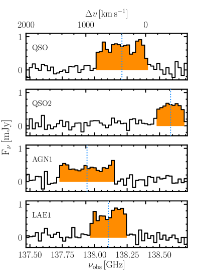
Figure 5: The four ALMA CO(5-4) line detections. The spectra at the CO(5-4) location for QSO, QSO2, AGN1, and LAE1 are shown from top to bottom, where the channels were binned to a width of 23.4 MHz ($\sim 51$ km s^-1). The rms noise for each spectra is listed in Table LABEL:tab:CO54. The line emissions above $2\times{\rm rms}$ used to compute quantities in Table LABEL:tab:CO54 are highlighted in orange. The velocity shift of the top x-axis are computed with respect to the QSO systemic redshift ($z=3.164$) obtained from C IV (Arrigoni Battaia et al. 2018a). We consider the first moment of the CO(5-4) detections as new systemic redshifts. In each panel, the vertical dotted blue line indicates such $z_{\rm CO(5-4)}$, which we use as reference redshift to derive the first moment maps (redshifts listed in Table LABEL:tab:CO54).

Table 3: CO(5-4) detections from ALMA, and their derived galaxy properties.

	QSO	QSO2	AGN1	LAE1
RMS noise per 23.4 MHz [${\rm\mu Jy}$]	118	117	133	103
SNRa	22.2	12.4	11.3	18.0
$z_{\rm CO(5-4)}^{\rm b}$	$3.1695\pm 0.0008$	$3.1582\pm 0.0006$	$3.1777\pm 0.0009$	$3.1727\pm 0.0007$
CO(5-4) line width [km s-1]c	$418\pm 101$	$211\pm 103$	$443\pm 202$	$246\pm 96$
$I_{\rm CO(5-4)}$ [Jy km s-1]	$0.43\pm 0.03$	$0.22\pm 0.02$	$0.28\pm 0.03$	$0.34\pm 0.02$
$L_{\rm CO(5-4)}$ [$10^{7}$ L⊙]	$4.5\pm 0.3$	$2.3\pm 0.2$	$2.9\pm 0.3$	$3.6\pm 0.2$
$L_{\rm CO(5-4)}^{\prime}$ [$10^{9}$ K km s-1 pc2]	$7.5\pm 0.4$	$3.9\pm 0.3$	$4.8\pm 0.5$	$6.0\pm 0.3$
$L_{\rm CO(1-0)}^{\prime}$ [$10^{9}$ K km s-1 pc2]d	$18.7\pm 1.1$	$9.6\pm 0.8$	$12.1\pm 1.3$	$14.9\pm 0.8$
2mm major axis [$\arcsec$]e	$1.07\pm 0.04$	$1.68\pm 0.21$	$1.12\pm 0.07$	$1.06\pm 0.05$
2mm minor axis [$\arcsec$]e	$0.98\pm 0.03$	$1.29\pm 0.14$	$1.04\pm 0.06$	$1.03\pm 0.05$
2mm dec. major axis [$\arcsec$]f	$0.52\pm 0.09$	$1.39\pm 0.27$	$0.64\pm 0.16$	$0.52\pm 0.17$
2mm dec. minor axis [$\arcsec$]f	$0.30\pm 0.15$	$0.89\pm 0.22$	$0.44\pm 0.19$	$0.43\pm 0.14$
R2mm [kpc]g	$2.0\pm 0.3$	$5.3\pm 1.0$	$2.4\pm 0.6$	$2.0\pm 0.6$
CO(5-4) major axis [$\arcsec$]e	$1.30\pm 0.11$	$1.67\pm 0.15$	$1.75\pm 0.18$	$1.39\pm 0.11$
CO(5-4) minor axis [$\arcsec$]e	$1.12\pm 0.09$	$1.36\pm 0.11$	$1.57\pm 0.15$	$1.29\pm 0.10$
CO(5-4) dec. major axis [$\arcsec$]f	$0.78\pm 0.20$	$1.33\pm 0.20$	$1.41\pm 0.23$	$0.95\pm 0.19$
CO(5-4) dec. minor axis [$\arcsec$]f	$0.49\pm 0.27$	$0.89\pm 0.18$	$1.21\pm 0.22$	$0.78\pm 0.17$
RCO(5-4) [kpc]g	$3.0\pm 0.8$	$5.1\pm 0.8$	$5.4\pm 0.9$	$3.6\pm 0.7$
$L_{\rm bol}$ [erg s-1]h	$(4.6\pm 0.2)\times 10^{47}$	$(8.8\pm 0.9)\times 10^{45}$	$(1.0\pm 0.5)\times 10^{46}$	$(1.3\pm 0.2)\times 10^{45}$
$L_{\rm IR}$ [$10^{12}$ L⊙]i	$4.7\pm 0.2$	$7.3\pm 1.9$	$3.0\pm 1.0$	$1.2\pm 0.2$
$L_{\rm IR}^{\rm total}$ [L⊙]l	$(1.7\pm 0.1)\times 10^{14}$	$(7.8\pm 2.3)\times 10^{12}$	$(1.0\pm 0.3)\times 10^{13}$	$(1.2\pm 0.2)\times 10^{12}$
SFR [M⊙ yr-1]m	$521\pm 74$	$183\pm 49$	$104\pm 21$	$50\pm 11$
SFRIR [M⊙ yr-1]n	$700\pm 30$	$1087\pm 283$	$447\pm 149$	$179\pm 30$
$M_{\rm dust}$ [M⊙]h	$(6.7\pm 1.3)\times 10^{8}$	$(1.5\pm 0.4)\times 10^{8}$	$(5.7\pm 1.3)\times 10^{8}$	$(1.6\pm 0.4)\times 10^{9}$
$M_{\rm dust}$ [M⊙]o	$(9\pm 3)\times 10^{8}$	$(3\pm 2)\times 10^{8}$	$(5\pm 2)\times 10^{8}$	$(4\pm 2)\times 10^{8}$
$M_{\rm H_{2},CO}$ [M⊙]p	$(1.5\pm 0.1)\times 10^{10}$	$(7.7\pm 0.7)\times 10^{9}$	$(1.0\pm 0.1)\times 10^{10}$	$(1.2\pm 0.1)\times 10^{10}$
$r_{\rm H_{2},dust}$ q	$22\pm 4$	$51\pm 14$	$18\pm 4$	$8\pm 2$
$M_{\rm star}$ [M⊙]r	$(1.2\pm 0.8)\times 10^{11}$	$(1.4\pm 0.4)\times 10^{10}$	$(1.1\pm 0.3)\times 10^{10}$	$(4.0\pm 0.5)\times 10^{9}$
$M_{\rm DM}$ [M⊙]s	$(6.9_{-5.6}^{+19.4})\times 10^{12}$	$(6.8\pm 1.0)\times 10^{11}$	$(6.0_{-1.6}^{+0.7})\times 10^{11}$	$(3.7_{-0.2}^{+0.3})\times 10^{11}$

Figure 6 shows cutouts of $7\arcsec\times 7\arcsec$ (or about 53 kpc $\times$ 53 kpc) of the moment zero, first and second moment maps, together with the continuum at each source position. As can be seen from this figure, the 2 mm continuum and the CO(5-4) emission are found at consistent sky locations within uncertainties. For this reason and to avoid confusion, in this work we only report the coordinates for the continuum (Table LABEL:tab:Interf).

The sizes of the 2mm continuum and CO(5-4) emitting regions are estimating by performing a 2D fit of the continuum and CO(5-4) moment zero maps. The fit is obtained using the task imfit within CASA, selecting a rectangular region of $4\arcsec\times 4\arcsec$ around each source. We fit a 2D Gaussian profile with the centroid, major and minor axis, position angle, and integrated flux as free parameters.

All the observed sizes from the fits are in the range $1.1\times-1.8\times$ of the synthesized beams, with all the observed CO(5-4) emitting regions on scales $\gtrsim 1.3$ the beam size. Given the high S/N of the detections, all the CO(5-4) emissions are therefore resolved (e.g., Decarli et al. 2018). The effective radius of each CO(5-4) emitting region, defined as the major semiaxis, is found to be $R_{\rm CO(5-4)}=3.0\pm 0.8,5.1\pm 0.8,5.4\pm 0.9,3.6\pm 0.7$ kpc, respectively for QSO, QSO2, AGN1, and LAE1. Hence QSO has likely the most compact host molecular reservoir down to the current depth of the observations. QSO2 has also the continuum resolved on comparable sizes to its CO(5-4) emission, $R_{\rm 2mm}=5.3\pm 1.0$ kpc. All these size measurements are reported in Table LABEL:tab:CO54, and in section 8 we discuss them in comparison with values from the current literature.

In addition, there are hints for resolved kinematics within each source. Indeed, there are symmetric blue and red shifts within the first moment maps of QSO2, AGN1, and LAE1 at the location of the highest S/N in the zero moment maps. Similar kinematic features have been reported in other high-$z$ quasars and have been interpreted as rotation (e.g., Bischetti et al. 2021). The line of nodes of these tentative rotation-like features was constrained by fitting a simple rotational curve to each object. Specifically, we perform chi-square minimization to estimate the position angle of the major axis, defined as the angle taken in the anticlockwise direction between the north direction in the sky and the major axis of the galaxy. The rotational curve were assumed to follow the simplest function, the arctan (Courteau 1997), which is flexible enough to reasonably describe $z\gtrsim 1$ rotating galaxies (e.g., Miller et al. 2011; Swinbank et al. 2012). We follow the procedures described in Chen et al. (2017) to project the one-dimensional arctan function to two-dimensional, and run MCMC with the EMCEE Python package (Foreman-Mackey et al. 2013) to fit the velocity maps and obtain posterior probability distributions. Because the asymptotic velocity and inclination angle are essentially degenerate for our data quality, we treat these two as a single parameter in the fit. As a result, the position angles of the major axis are $14^{+4}_{-5}$, $50^{+22}_{-22}$, and $120^{+9}_{-40}$ degrees for QSO2, AGN1, and LAE1, respectively. We highlight the obtained line of nodes (magenta) in Figure 6 and list in Table LABEL:tab:Angles the angles $\phi$ defining these directions in the reference frame East of North, together with their uncertainties. Table LABEL:tab:Angles also lists the angles $\theta$ between the spin directions of QSO2, AGN1, and LAE1 with respect to the direction to the QSO on the projected plane. For each companion source we found that its line of nodes (spin) is almost perpendicular (parallel) to its direction to the QSO, though with large uncertainties.

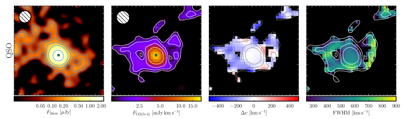
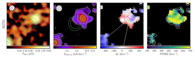
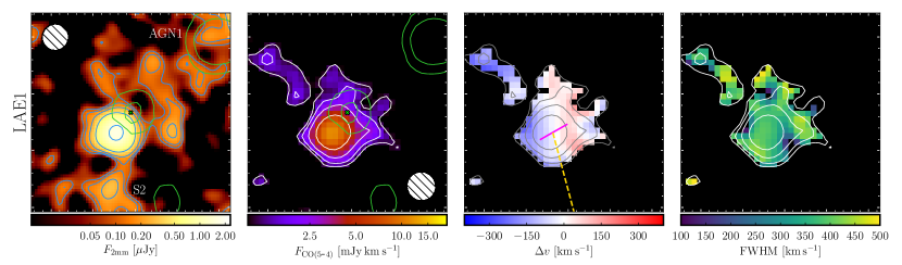
Figure 6: ALMA continuum and CO(5-4) moment maps for each line detected source, QSO, QSO2, AGN1, and LAE1. Each panel is a cutout of $7\arcsec\times 7\arcsec$ (or about 53 kpc $\times$ 53 kpc). The contours indicate the 2, 3, 5, 10, and 30$\sigma$ isophotes, and the 2, 3, 5, and 10$\sigma$ isophotes, respectively for the continuum and the line moment zero maps. The contours on the first and second moments show the isophotes from the moment zero cutout. The green cross shows the Ly$\alpha$ location of each source as determined with the available MUSE data (Arrigoni Battaia et al. 2018a). In addition, for AGN1 and LAE1, which are affected by large offset between Ly$\alpha$ and ALMA observations, we indicate the 20 and 30$\sigma$ contours for the Ly$\alpha$ (green). The size of the synthesized beam is shown on the continuum and on the line moment zero maps. As can be seen from the variation of the velocity shift and FWHM, there are hints for marginally resolved kinematics. On the first moment maps of QSO2, AGN1, and LAE1, we highlight the line of nodes (magenta). For these sources we also indicate the direction to the QSO (yellow). For AGN1 we also show the direction to LAE1 (gray).

Table 4: Angle measurements (in the reference frame East of North).

ID	$\phi^{\rm a}$	$\theta^{\rm b}$	$\phi^{\rm c}_{\rm off}$
	(deg)	(deg)	(deg)
QSO2	14${}^{+4}_{-5}$	8${}^{+4}_{-5}$	14$\pm$39
AGN1	50${}^{+22}_{-22}$	28${}^{+22}_{-22}$	50$\pm$76
LAE1	120${}^{+9}_{-40}$	15${}^{+9}_{-40}$	96$\pm$28

To further inspect these velocity shifts, we produced zero moment maps within several velocity ranges. Figure 7 shows an example of these maps, highlighting the location of the CO(5-4) emission at negative (blue contours), positive (red), and around zero (yellow) velocities with respect to the 2 mm continuum emission. This test further confirms our previous analysis. In particular, QSO does not show a spatial offset between the emission at positive and negative velocities. The three peaks in its integrated CO(5-4) spectrum seems therefore not associated with three distinct components at this spatial resolution. On the other hand, we find significant offsets between emission at negative and positive velocities of $0.4\pm 0.2$, $0.4\pm 0.2$, and $0.5\pm 0.1$ arcsec for QSO2, AGN1, and LAE1, respectively. As a sanity check, the directions of these shifts are consistent with the major axis computed by fitting the moment maps. However, they have larger uncertainties as they are not based on a fit to the full data information. Specifically, the angles between the negative and positive peak are found to be $14\pm 39$, $50\pm 76$, and $96\pm 28$ degrees for QSO2, AGN1, and LAE1, respectively. We also list these angles in Table LABEL:tab:Angles.

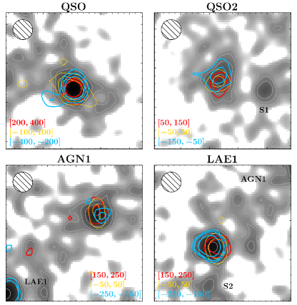
Figure 7: CO(5-4) contours from zero moment maps within different velocity ranges (see colored legend on each panel) overlayed on the ALMA continuum maps for the sources detected in CO(5-4): QSO, QSO2, AGN1, and LAE1. Each panel is $7\arcsec\times 7\arcsec$ (or about 53 kpc $\times$ 53 kpc) as in Fig 6. The contours are drawn at 3, 5, and 7$\sigma$, if possible.

Finally, Figure 6 compares the location of the centroid of the Ly$\alpha$ emission of each source with the millimeter observations. While the QSO and QSO2 locations are consistent at different wavelengths, AGN1 and LAE1 show measurable shifts between the 2 mm continua (or CO(5-4) emission) and the Ly$\alpha$ emission. We estimate these to be 1.5$\arcsec$ (or $\sim 11.4$ kpc) and 0.9$\arcsec$ (or $\sim 6.8$ kpc), respectively for AGN1 and LAE1. These shifts are significant for both the ALMA and MUSE observations. We stress that we have verified the astrometric calibration of the MUSE observations presented in Arrigoni Battaia et al. (2018a) against the two available sources (one is QSO) in the GAIA DR2 catalogue (Gaia Collaboration et al. 2018) within the observations field-of-view. We found agreement between the astrometric calibration done using the SDSS DR12 catalogue (Alam et al. 2015) and the few GAIA sources, confirming the precision of astrometry of about one pixel of the IFU data ($\sim 0.2\arcsec$). We further note that the offsets of AGN1 and LAE1 are in opposite directions with respect to each other, which would require a rather weird distortion pattern throughout the data to cancel it out. Therefore, we are confident that the aforementioned shifts between millimeter observations and Ly$\alpha$ are real. We discuss these shifts in Section 6.

4 Estimated mass budget of the ELAN system

In this section we attempt a first estimate of the mass budget of this ELAN system, specifically within the dark-matter (DM) halo expected to host the system in a $\Lambda$CDM universe. We start by estimating in first approximation the stellar masses, dust masses, star formation rates, and molecular gas masses for the sources with confirmed association with the ELAN, i.e., QSO, QSO2, AGN1 and LAE1 (sections 4.1 and 4.2). We then show that the derived masses for each source are consistent with the dynamical masses estimated from the CO(5-4) line emission under the assumption of a reasonable inclination angle (section 4.3). In section 4.4.1, the estimated stellar masses are used to infer the DM halo mass of the system using the halo mass $M_{\rm DM}$ - stellar mass $M_{\rm star}$ relations in Moster et al. (2018). The inferred DM halo mass is found in agreement with the estimate from an orthogonal method using the projected distances and redshift differences of the sources (Tempel et al. 2014). We then discuss in section 4.4.2 the mass budget in the baryonic components, under several assumptions and also taking into account different baryon fractions. We conclude the section by forecasting the system evolution (section 4.5). In each section we discuss the limitations and assumptions of each method, and also indicate some of the needed datasets to refine our estimates.

4.1 Dust and stellar masses, and star formation rates

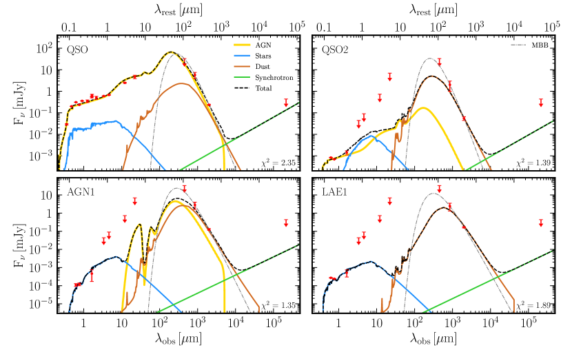
Figure 8: Observed spectral energy distribution (SED) for each CO(5-4) detected source, QSO, QSO2, AGN1, LAE1. We fit the data-points (red) with the SED fitting code CIGALE (Boquien et al. 2019; see section 4.1 for details). We show the best-fit model (black dashed line), and its individual components: stellar emission (blue), dust emission (brown), AGN emission (yellow), synchrotron radiation (green). We report the $\chi^{2}$ of the best-fit model in the bottom right corner. Table LABEL:tab:CO54 lists some of the properties obtained from these fits. For each source we also indicate a modified black-body with T=40 K for the FIR emission (dot-dashed gray line; see section 4.1).

The dust and stellar masses, as well as the star formation rates (SFRs) are estimated by fitting the spectral energy distribution (SED) of each source, as usually done in the literature (e.g., Calistro Rivera et al. 2016; Circosta et al. 2018). The SEDs are built using the data described in the previous sections, together with the information at $3.4,4.6,12,22$ $\mu$m from the AllWISE source Catalog, and at $1.4$ GHz from VLA FIRST (Becker et al. 1994). These additional data-points are listed in Appendix E (Table LABEL:tab:app_phot).

We rely on the SED fitting code CIGALE (v2018.0, Boquien et al. 2019), which covers the full range of the current datasets, from rest-frame ultraviolet (UV) to radio emission. CIGALE fits simultaneously all this wavelength range imposing energy balance between the UV and the infrared (IR) emission (reprocessed dust emission), while decomposing the SED into different physically motivated components. This energy balance is critical for getting meaningful stellar masses with few datapoints. For our specific case, we select (i) an AGN component (accretion disk plus hot dust emission; Fritz et al. 2006), (ii) dust emission from star-forming regions (Draine & Li 2007; Draine et al. 2014), (iii) radio synchrotron emission, and (iv) stellar emission from the host galaxy, which is modelled by an exponentially declining star formation history (SFH), the simple stellar population models of Bruzual & Charlot (2003), a Chabrier initial mass function (Chabrier 2003), and a modified starburst attenuation law (based on Calzetti et al. 2000 and Leitherer et al. 2002). Details on these specific models and a comparison with other models implemented in CIGALE are discussed in Boquien et al. (2019). The parameters available for each model using the code’s notation and the ranges explored by our fit are:

• AGN emission: this model has seven parameters, five of which are left free to explore all the values allowed by CIGALE. The remaining parameters are the AGN fraction ($fracAGN$; defined as the ratio of the AGN luminosity to the sum of the AGN and dust luminosities) and the angle between equatorial axis and line-of-sight ($psy$). We let $fracAGN$ vary between 0 and 1 in steps of 0.05. $psy$ is allowed to vary between 0.001 and 40.100 for type-2 AGN, and between 50.100 and 89.990 for type-1 AGN.

• dust emission: this model has four parameters (mass fraction of PAH, minimum radiation field, power-law slope, fraction of dust illuminated) which are left free to explore all the values allowed by CIGALE.

• synchrotron emission: this model has two parameters, the value of the FIR-to-radio coefficient (Helou et al. 1985) and the slope of the synchrotron power-law. Given the absence of tight constraints in the radio for any of the sources we fixed the slope to -1.0 (as observed in sources within other ELANe, e.g., Decarli et al. 2021) and the ratio to an arbitrary value satisfying the VLA FIRST upper limits. This portion of the SED has to be considered simply as illustrative.

• stellar emission: the SFH is modelled with two parameters, age and e-folding time $\tau$. The age is allowed to vary between 0.1 Gyr and 2 Gyr (about the age of the universe at $z=3.164$) in step of 0.1 Gyr, while $\tau$ can vary between 0.1 and 10 Gyr in step of 0.1 Gyr. The attenuation model is set up so that the final $E(B-V)$ is between 0 and 3. All the other eight parameters are kept to the default values.

In addition, for high-redshift sources, CIGALE applies a correction to rest-frame UV data for the attenuation from the foreground intergalactic medium following Meiksin (2006).

In the continuum fit we do not include the nebular emission component, for which CIGALE has built-in templates. Indeed, we find that the nebular $Ly\alpha$ line emission from some of these sources is displaced with respect to the continuum (e.g., section 3.5). The best-fit models obtained following this procedure using the pdf_analysis module in CIGALE are shown in Figure 8, together with their $\chi^{2}$ values and the observed data-points. The likelihood-weighted output dust and stellar masses, and the SFRs together with their likelihood-weighted uncertainties are listed in Table LABEL:tab:CO54. We stress that these uncertainties do not include systematic errors due to the models used, a priori assumptions on the nature of the sources, and the discrete coverage of the parameter space.

Specifically, we find dust masses in the range $M_{\rm dust}=1.5$-$16\times 10^{8}$ M_⊙, with LAE1 being the most dust rich object in the system. As an additional check, we computed the dust masses using a modified black body model, assuming (i) a dust temperature $T_{\rm dust}=40$ K , (ii) a dust opacity at 850 $\mu$m of $\kappa_{\rm d}=0.43$ cm² g^-1 (Li & Draine 2001), and (iii) a fixed dust emissivity power-law spectral index $\beta$ derived from the SMA and ALMA continuum. We find $\beta=2.4\pm 0.1,2.9\pm 0.2,2.3\pm 0.2,1.8\pm 0.2,$ for QSO, QSO2, AGN1, and LAE1, respectively. The values for QSO, QSO2, and AGN1 are on the high side of the values usually found for high-redshift quasars (e.g., $\beta=1.95\pm 0.3$, Priddey & McMahon 2001; $\beta=1.6\pm 0.1$, Beelen et al. 2006) or dusty star-forming galaxies (e.g., $\beta=2.0\pm 0.2$ , Magnelli et al. 2012), and are consistent with the value of $\beta=2.5$ used to fit SEDs of HzRGs (Falkendal et al. 2019). The dust masses derived with this method are $M_{\rm dust}=(9\pm 3)\times 10^{8}$ M_⊙, $(3\pm 2)\times 10^{8}$ M_⊙, $(5\pm 2)\times 10^{8}$ M_⊙, and $(4\pm 2)\times 10^{8}$ M_⊙, respectively for QSO, QSO2, AGN1, and LAE1. Hence, they agree with the CIGALE output (LAE1 within 2$\sigma$). The obtained dust masses are (i) in the range usually derived in high-redshift quasars hosts from $z\sim 2$ up to $z\sim 7$ (e.g., Weiß et al. 2003; Schumacher et al. 2012; Venemans et al. 2016), (ii) within the typical range for high-redshift dusty, star-forming galaxies (e.g., Casey et al. 2014; Dudzevičiūtė et al. 2020), and (iii) similar to what is reported for HzRGs (few times $10^{8}$ M_⊙ assuming $T\sim 50$ K; e.g., Archibald et al. 2001).

The stellar masses are found to be in the range ${M_{\rm star}=4.0\times 10^{9}}$ M_⊙ and $1.2\times 10^{11}$ M_⊙, with QSO being hosted by the most massive galaxy in this system, as expected (Arrigoni Battaia et al. 2018a). The other associated galaxies are about 10$\times$ less massive (Table LABEL:tab:CO54). Given that QSO greatly outshine its host galaxy the stellar mass derived with CIGALE has to be taken with caution. However, we show in section 4.3 that the dynamical mass derived from CO(5-4) is consistent with the presence of such a massive galaxy. The obtained stellar masses agree well with literature values for quasar hosts (e.g., $\sim 10^{11}$ M_⊙, Decarli et al. 2010) and the more massive and IR detected LAEs (e.g., $10^{9}-10^{10.5}$ M_⊙, Ono et al. 2010) found at similar redshifts. The QSO host has a stellar mass consistent with the median stellar mass for the Spitzer $1<z<5.2$ HzRGs ($\sim 10^{11}$ M_⊙; De Breuck et al. 2010).

With these estimates, the dust-to-stellar mass ratios are $M_{\rm dust}/M_{\rm star}=0.006\pm 0.004,0.010\pm 0.004,0.05\pm 0.02,0.4\pm 0.1$, for QSO, QSO2, AGN1, and LAE1, respectively. These values are in agreement within uncertainties with observations of main-sequence and starburst galaxies at these redshifts (in the range $0.001-0.1$, e.g., da Cunha et al. 2015; Donevski et al. 2020), except LAE1 which has a larger value. Given the similarity with the SED of AGN1, this tension could be solved by including an AGN component in the SED fit for LAE1. The current dataset does not show a clear evidence for AGN activity in LAE1, but it could be obscured. X-rays observations are therefore needed to verify the nature of this source.

Further, CIGALE determined the instantaneous SFR for each source, indicating ${\rm SFR}=521\pm 74,183\pm 49,104\pm 21,50\pm 11$ M_⊙ yr^-1 for QSO, QSO2, AGN1, LAE1, respectively. These SFRs are in line with values from the literature. In particular, the SFR in the QSO host agrees well with values usually found in $z\sim 2-3$ quasars (e.g., Harris et al. 2016). We also computed the SFR from the total infrared (IR) emission using the rest-frame wavelength range $8-1000$ $\mu$m for the obtained SED. For this purpose, we used the relation (SFR${}_{\rm IR}/[M_{\odot}~{}{\rm yr}^{-1}])=3.88\times 10^{-44}(L_{\rm IR}/[{\rm erg~{}s^{-1}}])$ in Murphy et al. (2011), usually employed for high-redshift quasars (e.g., Venemans et al. 2017). This relation has been computed using Starburst99 (Leitherer et al. 1999) with a fixed SFR and a Kroupa initial mass function (Kroupa 2001), and assumes that the entire Balmer continuum is absorbed and re-radiated by dust in the optically thin regime. Applying this relation only to the IR luminosity $L_{\rm IR}$ computed excluding the AGN contribution (see Table LABEL:tab:CO54), results in ${\rm SFR}_{\rm IR}=700\pm 30,1087\pm 283,447\pm 149,179\pm 30$ M_⊙ yr^-1 for QSO, QSO2, AGN1, LAE1, respectively. These values are higher than the instantaneous SFRs, reflecting the longer timescales probed by the IR tracers.

Further, in Figure 9 we show the location of QSO, QSO2, AGN1, and LAE1 in the $L_{\rm IR}$ versus $L^{\prime}_{\rm CO(5-4)}$ plot in comparison to submillimeter galaxies (SMGs) and high-redshift quasars. The CO(5-4) line is known to be linked to $L_{\rm IR}$ through a relation of the form log${L_{\rm IR}=\alpha{\rm log}L^{\prime}_{\rm CO(5-4)}+\beta}$ from low to high-redshift (e.g., Greve et al. 2014; Daddi et al. 2015, dotted and dashed lines). Our sources are consistent with the scatter of known high-redshift sources (e.g., Valentino et al. 2020, blue line with intrinsic scatter), ensuring that the AGN-corrected $L_{\rm IR}$ obtained from the SED fitting are reasonable.

Summarizing, we find values for dust and stellar masses, and SFRs within the scatter of observations reported in the literature. Follow-up observations in the NIR and mm regimes are needed to lower the uncertainties on our estimates.

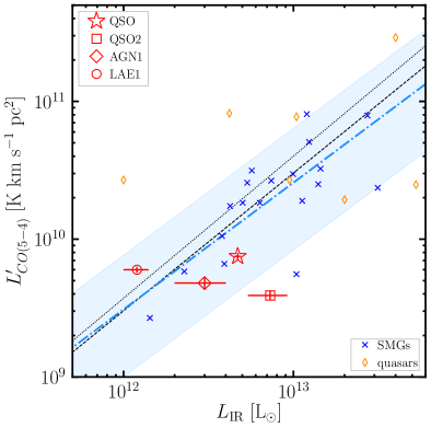
Figure 9: $L^{\prime}_{\rm CO(5-4)}$ versus $L_{\rm IR}$ plot. We compare the location of QSO, QSO2, AGN1, and LAE1 (red) with SMGs (compilation in Carilli & Walter 2013) and high-redshift quasars ($z\sim 2.5-6$; Barvainis et al. 1997; Guilloteau et al. 1999; Weiß et al. 2003; Carilli et al. 2007; Wang et al. 2007, 2010; Schumacher et al. 2012). We stress that $L_{\rm IR}$ for most of the high-redshift quasars is not corrected for a contribution from the AGN. We also indicate (i) the relation by Greve et al. (2014) obtained by fitting only low-redshift sources (no SMGs nor high-redshift quasars included; dotted line), (ii) the relation from Daddi et al. (2015) obtained by fitting from local spirals to SMGs (no high-redshift quasars considered; dashed line), and (iii) the relation from Valentino et al. (2020) (blue line with its intrinsic scatter), who updated the work by Daddi et al. (2015) using a larger galaxy sample (no high-redshift quasars considered).

4.2 Molecular gas masses derived from CO

It is common practice to obtain the molecular mass through the equation $M_{\rm gas}=\alpha L_{\rm CO(1-0)}^{\prime}$, with $\alpha$ being the CO luminosity-to-gas mass conversion factor and $L_{\rm CO(1-0)}^{\prime}$ the CO(1-0) luminosity in units of K km s^-1 pc² (e.g., Carilli & Walter 2013; Aravena et al. 2019). To use this equation, we assume $\alpha_{\rm CO}=0.8$ M_⊙ $({\rm K\,km\,s^{-1}\,pc^{2}})^{-1}$. This value has been derived for local ultra-luminous infrared galaxies (ULIRGs; e.g., Downes & Solomon 1998), and it is commonly used to calculate molecular gas masses in high-redshift quasars ($z\sim 2-7$; e.g., Riechers et al. 2006; Coppin et al. 2008; Carilli & Walter 2013; Venemans et al. 2017). As only the CO(5-4) line flux is available, we have to further assume a CO spectral line energy distribution (CO SLED) to derive how strong is the CO(1-0) transition. Current statistics show that the CO SLED of high-redshift quasars peaks at high-$J$ transition, CO(6-5) and CO(7-6), with a minimum flux ratio CO(5-4)/CO(1-0)$\sim 10$ (Weiss et al. 2007; Carilli & Walter 2013). Therefore, we derive the corresponding $L_{\rm CO(1-0)}^{\prime}$ assuming this ratio. The values obtained for the three AGN (QSO, QSO2, AGN1) are considered as possible upper limits (i.e. their CO SLED could be more excited; e.g., Weiß et al. 2007), while for LAE1 it is possibly a lower limit. For completeness we list the inferred CO(1-0) luminosities in Table LABEL:tab:CO54. We note that the adopted CO(5-4)/CO(1-0) corresponds to a $r_{51}=L_{\rm CO(5-4)}^{\prime}/L_{\rm CO(1-0)}^{\prime}=0.4$ (the range reported in Carilli & Walter (2013) is $r_{51}=0.69\pm 0.3$). This value is also consistent within 2$\sigma$ with the values reported for the spectrum obtained for $z>2$ gravitationally lensed dusty star-forming galaxies by Spilker et al. (2014) ($r_{51}=0.67\pm 0.20$), with the median value reported for 32 $z\sim 1.2-4.1$ luminous submillimeter galaxies ($r_{\rm 51}=0.32\pm 0.05$; Bothwell et al. 2013), the average value for 8 $z>2$ star forming galaxies ($r_{51}=0.44\pm 0.11$; Boogaard et al. 2020), and for the compilation of SMGs in Birkin et al. (2021) ($r_{51}=0.35\pm 0.08$).

Using the derived CO(1-0) luminosities and the assumed $\alpha_{\rm CO}$, the resulting gas masses $M_{\rm gas}$ are $(1.5\pm 0.1)\times 10^{10}$, $(7.7\pm 0.7)\times 10^{9}$, $(1.0\pm 0.1)\times 10^{10}$, and $(1.2\pm 0.1)\times 10^{10}$ M_⊙, respectively for QSO, QSO2, AGN1, and LAE1 (see also Table LABEL:tab:CO54). These values, though uncertain, are within the ranges reported in the literature for high-redshift quasars and dusty star-forming galaxies ($M_{\rm gas}={\rm few}\times 10^{10}(\alpha_{\rm CO}/0.8)$ M_⊙; e.g., Carilli & Walter 2013; Bothwell et al. 2013), and are also at the low-end of masses reported for HzRGs ($10^{10}-10^{11}$ M_⊙; e.g., Miley & De Breuck 2008).

When comparing the obtained molecular gas masses to the dust masses derived in Section 4.1, we find molecular-to-dust mass ratios $r_{\rm H_{2},dust}$ in the range 8 - 51 (see Table LABEL:tab:CO54), which are very low in comparison to the usually assumed gas-to-dust mass ratios for local galaxies ($\sim 100$; e.g., Draine et al. 2007; Galametz et al. 2011) and high-redshift massive star-forming galaxies ($\sim 100$; e.g., Riechers et al. 2013), even when correcting them for the fraction of gas in molecular form ($\sim 80$ %; e.g., Riechers et al. 2013). Interestingly, these values are more similar to what is seen in SMGs (e.g., $r_{\rm H_{2},dust}=28^{+7}_{-6}$; Kovács et al. 2006). Therefore, our measurement could be due to a real molecular gas deficiency or efficient dust absorption (i.e. larger dust opacities) in these sources, or could be related to the assumptions made to determine the molecular gas masses. Assuming a Milky-Way value of $\alpha_{\rm CO}\sim 4$ M_⊙ $({\rm K\,km\,s^{-1}\,pc^{2}})^{-1}$, the molecular-to-dust mass ratios increase, but still two sources (AGN1 and LAE1) have values reflecting a depletion of molecular gas. Less excited CO ladders would then be needed to increase our molecular mass estimates and thus alleviate the tension for these sources. It is clear that our measurements need to be refined with follow-up observations of additional CO transitions (especially at lower $J$; ALMA, NOEMA, J-VLA) or other molecular gas tracers (e.g., [CI]), to at least remove the uncertainties on the CO excitation ladder. For completeness, the $r_{\rm H_{2},dust}$ values are also listed in Table LABEL:tab:CO54.

4.3 Dynamical Masses from CO kinematics and sizes

In this section we outline rough estimates of the dynamical masses for QSO, QSO2, AGN1, and LAE1, using the kinematics and sizes of the CO(5-4) emitting region. In turn, these dynamical masses can be compared to the galaxies mass budget derived in the previous sections. As rotation-like signatures are present in most of the CO(5-4) maps (Section 3.5), the bulk of the molecular gas is assumed to be in a disk with an inclination $i$. This approach is common practice in the study of unresolved line tracers of molecular gas associated with high-redshift quasars (e.g., Decarli et al. 2018). In this framework, the dynamical mass can be obtained as $M_{\rm dyn}=G^{-1}R_{\rm CO(5-4)}({\rm FWHM}/{\rm sin}(i))^{2}$ (Willott et al. 2015), where $G$ is the gravitational constant, $R_{\rm CO(5-4)}$ is the size of the CO(5-4) emitting region and FWHM is its line width. As the quality of our data does not allow an estimate of the inclination angle (Section 3.5), we assume the mean inclination angle for randomly oriented disks $\langle{\rm sin}(i)\rangle=\pi/4$ (e.g., Law et al. 2009), obtaining $M_{\rm dyn}=(1.9\pm 0.8)\times 10^{11},(8.5\pm 6.7)\times 10^{10},(3.9\pm 2.9)\times 10^{11},(8.2\pm 5.2)\times 10^{10}$ M_⊙ for QSO, QSO2, AGN1, and LAE1, respectively. These dynamical masses are consistent within their large uncertainties to the sum of the galaxy different mass components (i.e., molecular, stellar, dust), also considering the contribution of a Navarro-Frenk-White (NFW; Navarro et al. 1997) dark-matter component within $R_{\rm CO(5-4)}$ assuming the concentration-halo mass relation in Dutton & Macciò (2014).

For QSO2, AGN1, and LAE1, the dynamical masses including some pressure support can be further assessed, using the observed asymptotic rotational velocities $v_{\rm rot}^{\rm obs}$ obtained from the 2D fit of their first moment maps described in section 3.5, and the velocity dispersion $\sigma$ within their effective radii in their second moment maps. In this framework, $M_{\rm dyn}=2R_{\rm CO(5-4)}(v_{\rm rot}^{2}+\sigma^{2})/G$ (e.g., Smit et al. 2018), where $v_{\rm rot}=v_{\rm rot}^{\rm obs}/{\rm sin}(i)$, assuming again $\langle{\rm sin}(i)\rangle=\pi/4$. Using the computed values of $v_{\rm rot}^{\rm obs}=170^{+30}_{-60},190^{+60}_{-60},190^{+50}_{-40}$ km s^-1 and $\sigma=119\pm 89,259\pm 153,156\pm 138$ km s^-1, we obtain $M_{\rm dyn}=1.4^{+0.6}_{-0.7}\times 10^{11},3.1^{+2.1}_{-2.1}\times 10^{11},1.4^{+0.8}_{-0.8}\times 10^{11}$ M_⊙ for QSO2, AGN1 and LAE1, respectively. These masses are consistent with the previously determined values.

Notwithstanding the aforementioned fair agreement between the estimated dynamical masses and the mass budget for each galaxy, we note that the obtained dynamical masses are usually providing larger mass estimates, especially for AGN1. This tentative mismatch can however be evidence of turbulence injection in the molecular reservoir due to different physical processes expected in galaxy evolution: infall of gas at velocities of hundreds of km s^-1, stellar and AGN feedback. In other words, turbulence due to these processes could explain the large velocity dispersions seen in the four CO(5-4) detected objects (Figure 6). Higher resolution observations, exploiting the ALMA longest baselines, are required to firmly assess the dynamical masses of these sources.

4.4 The system mass budget

In this section we present an estimation of the mass budget of the whole system and compare that to the cosmic baryon fraction. To compute the dark matter and baryonic (stars, molecular gas, dust, atomic gas) components, we rely on the previously obtained values and on several additional assumptions which are needed to overcome the limitations of the current observations.

We assume that the sources detected by ALMA, i.e., QSO, QSO2, AGN1, LAE1, are the most massive objects in this system, and neglect the contributions from additional sources. It will be clear that additional satellite masses are well accommodated within the final error estimates of our discussion.

4.4.1 The dark matter component

We used two methods to esimate the total dark matter (DM) halo mass for the system. First, we interpolate the halo mass $M_{\rm DM}$ - stellar mass $M_{\rm star}$ relations in Moster et al. (2018) for the redshift of interest here, to obtain the expected $M_{\rm DM}$ for each of the sources. The resulting halo masses are in the range $3.7\times 10^{11}$ M${}_{\odot}\leq M_{\rm DM}\leq 6.9\times 10^{12}$ M_⊙ (Table LABEL:tab:CO54). To get a total halo mass, we then simply sum the obtained masses, finding $M_{\rm DM}^{\rm total}=(8.6^{+19.4}_{-5.6})\times 10^{12}$ M_⊙, with 81 % of the DM mass due to the QSO halo. The large uncertainties here are due to the well-known challenges in assessing the stellar mass of the bright quasar hosts (e.g., Targett et al. 2012), and the larger scatter in halo mass for stellar masses close to the peak efficiency of star formation (Moster et al. 2018).

Secondly, we estimate the dynamical mass of the system as done for low-redshift groups and clusters using the formalism of Tempel et al. (2014). We apply this method to the studied ELAN using the ALMA data (systemic redshifts and positions) for each source. This method assumes that (i) the system is already virialized, (ii) dynamical symmetry, so that the true velocity dispersion $\sigma_{v}$ of the system is $\sqrt{(}3)\times$ the velocity dispersion along the line-of-sight, and (iii) a gravitational radius $R_{\rm g}$ obtained as in Binney & Tremaine (2008), while assuming a DM density profile (here a NFW) and the observed spatial dispersion in the plane of the sky (equation 4 in Tempel et al. 2014). The total dynamical mass is then given by ${M_{\rm dyn}^{\rm tot}=2.325\times 10^{12}(R_{\rm g}/{\rm Mpc})(\sigma_{v}/100\,{\rm km\,s^{-1}})^{2}}$ M_⊙. The observed projected distances and redshift differences result in $R_{\rm g}=354\pm 76$ kpc and $\sigma_{v}=515\pm 39$ km s^-1, and therefore in $M_{\rm dyn}^{\rm tot}=(2.2\pm 0.3)\times 10^{13}$ M_⊙. If we then assume a maximum baryon fraction equal to the cosmic baryon fraction, the total DM mass for the system is $M_{\rm DM}^{\rm total}=(1.8\pm 0.3)\times 10^{13}$ M_⊙ .

The two obtained values for the DM mass agree within uncertainties, with the dynamical mass on the high side of the first estimate possibly due to a lack of virialization in this system. Therefore, we can consider the stellar masses obtained in section 4.1 to be reasonable. In the remainder of the analysis we will consider both estimates of DM masses, which overall suggest that this ELAN is sitting in a DM halo of $\sim 10^{13}$ M_⊙. Interestingly, this halo mass is on the high side of the halo mass measurements presented in the literature for quasars (usually between $10^{12}$ and $10^{13}$ M_⊙ at $z\sim 3$; e.g., Shen et al. 2007; Kim & Croft 2008; Trainor & Steidel 2012; Eftekharzadeh et al. 2015), possibly further confirming that ELANe are associated with the most massive and therefore overdense quasar systems (Hennawi et al. 2015; Arrigoni Battaia et al. 2018a). In addition, this ELAN inhabits a DM halo as massive as those expected for HzRGs (e.g., Stevens et al. 2003), bright LABs (Yang et al. 2010), and SMGs (e.g., Wilkinson et al. 2017; Lim et al. 2020, but see Garcia-Vergara et al. 2020), revealing that it is among the most massive systems at its redshift.

4.4.2 The baryonic components

For the baryon budget, we proceed by simply adding up the masses of each component for QSO, QSO2, AGN1, and LAE1 and propagating their errors, finding ${M_{\rm star}^{\rm total}=(1.5\pm 0.8)\times 10^{11}}$ M_⊙, ${M_{\rm dust}^{\rm total}=(3.0\pm 0.4)\times 10^{9}}$ M_⊙, $M_{\rm H_{2}}^{\rm total}={(4.5_{-0.2}^{+17.9})\times 10^{10}}$ M_⊙, for the total stellar, dust, and molecular masses. In the error budget for the molecular mass we include the large uncertainty (a factor of 5) on $\alpha_{\rm CO}$. This large uncertainty should also include the possibility of molecular gas extending on scales larger than the body of galaxies as seen for example in HzRGs environments (e.g., Emonts et al. 2016; see Section 8 for discussion). From the mass budget we then miss the atomic gas components at different temperatures, i.e., cold ($\sim 100$ K), cool ($\sim 10^{4}$ K), and warm-hot ($>10^{5}$ K).

We can predict the amount of cold atomic gas by assuming that the interstellar-medium molecular gas fraction is $\sim 80$ % at high-redshift (e.g., Riechers et al. 2013), and in turn that the cold atomic gas fraction is therefore $f_{\rm cold}\sim 20$ %. This is also consistent with current estimates for such massive halos at $z\sim 3$ from semi-empirical models of galaxy evolution (e.g., Popping et al. 2015). We therefore include in the budget a total cold atomic mass of $M_{\rm HI}^{\rm cold}=(0.9_{-0.1}^{+3.6})\times 10^{10}$ M_⊙. This prediction could be tested by targeting the [CII] emission at 158 $\mu$m with e.g., ALMA (e.g., Fujimoto et al. 2020).

To derive a total cool gas mass, we can instead rely on the large-scale Ly$\alpha$ emission detected with VLT/MUSE in Arrigoni Battaia et al. (2018a). Given that the projected maximum distance of the Ly$\alpha$ emission is comparable with the obtained virial radii, we assume that all the Ly$\alpha$ nebula sits within the halo. This is also in agreement with the discussion in Arrigoni Battaia et al. (2018a), who argued that the Ly$\alpha$ emission traces the motions of substructures accreting within the bright quasar massive halo. We then assume that the visible Ly$\alpha$ emitting gas is the densest cool gas in the halo, and thus the one contributing to most of its mass. The cool gas mass can then be estimated as $M_{\rm cool}^{\rm total}=A\,m_{\rm p}/X\,f_{C}\,N_{\rm H}$ (Hennawi & Prochaska 2013), where $A$ is the projected area on the sky covered by the ELAN in cm² ($609.36$ arcsec² within the $2\sigma$ isophote in Arrigoni Battaia et al. 2018a), $m_{\rm p}$ is the proton mass, $X=0.76$ is the hydrogen mass fraction (e.g., Pagel 1997), $f_{\rm C}$ is the cool gas covering factor within the ELAN, and $N_{\rm H}$ is the total hydrogen column density of the emitting gas. We assume (i) $f_{\rm C}=1$ as it has been shown that the observed morphology of extended Ly$\alpha$ nebulae can be reproduced if $f_{\rm C}\gtrsim 0.5$ (Arrigoni Battaia et al. 2015b), and (ii) a constant ${\rm log}(N_{H}/{\rm cm^{-2}})=20.5\pm 1.0$, which is the median value found by Lau et al. (2016) for optically thick absorbers in $z\sim 2$ quasar halos (see their Figure 15). For this latter value we assume an error which encompasses the large uncertainties in some of those authors data-points. Inserting these values in the aforementioned relation gives $M_{\rm cool}^{\rm total}=1.2_{-1.0}^{+10.5}\times 10^{11}$ M_⊙. We stress that this calculation neglects additional cool gas within the halo not emitting Ly$\alpha$ above the sensitivity of the observations in Arrigoni Battaia et al. (2018a). However, the current area of the nebula covers 42% or 25% of the projected halo for the Moster et al. or the Tempel et al. calculation, respectively. Even if we assume the full halo to be covered by Ly$\alpha$ emission the total mass would increase by a factor of 2.4 or 4, respectively, thus falling within the errors of the previous measurement. Interestingly, the obtained $M_{\rm cool}^{\rm total}$ agrees well with cool gas masses reported for $z\sim 2-3$ quasars halos ($M_{\rm cool}^{\rm total}>10^{10}$ M_⊙; e.g., Prochaska et al. 2013; Lau et al. 2016), and reported for other ELANe ($1.0\times 10^{11}$ M${}_{\odot}<M_{\rm cool}^{\rm total}<6.5\times 10^{11}$ M_⊙; Hennawi et al. 2015).

Figure 10: The baryonic mass budget for the whole system within its virial radius, divided in its stellar, dust, molecular, atomic (cold, cool, and warm-hot) components. Each component has been calculated assuming a halo baryon fraction equal to the cosmic value of 15.6 % (Planck Collaboration et al. 2020). The fractions are computed for both $M_{\rm DM}$ values obtained in this work: using the relations in Moster et al. (2018) and following the formalism in Tempel et al. (2014). See Section 4.4 for details.

Figure 10 summarizes the discussed baryonic components as fractions of the total mass of the system, which has been derived by assuming a halo baryon fraction equal to the cosmic value (15.6 %). It is clear that the stars, dust, molecular, cold and cool atomic components add up to a small fraction of the cosmic value, with 21 % or 10 % of the baryons in these constituents depending on the DM mass considered, Moster et al. or Tempel et al., respectively. These values, though uncertain, are lower than the estimated value reported for $z\sim 2$ quasars ($56\%$; Lau et al. 2016). We can easily explain these differences with the larger halo masses derived in this work with respect to the assumed halo mass in Lau et al. (2016) ($M_{\rm DM}=10^{12.5}$ M_⊙). In other words, we find similar baryonic masses but in a halo which is $2.7\times$ or $5.9\times$ more massive. If all the quasars in Lau et al. (2016) inhabit DM halos as massive as the one of this ELAN, they would have a similar baryon budget.

As expected from galaxy formation theories (e.g., Dekel & Birnboim 2006), our analysis suggests that the rest of the baryonic mass is in a warm/hot phase which permeates the halo of this massive system. Assuming a halo baryon fraction equal to the cosmic value, this warm/hot phase would represent a reservoir as massive as $M_{\rm warm-hot}^{\rm total}=(1.3_{-0.2}^{+1.2})\times 10^{12}$ M_⊙ or $M_{\rm warm-hot}^{\rm total}=(3.1_{-0.1}^{+1.1})\times 10^{12}$ M_⊙, for Moster et al. and Tempel et al. DM calculations, respectively (Figure 10). The warm-hot phase together with the cool phase would then represent 87 % or 94 % of the baryon fraction.

We can further gain some intuition on the halo gas physical properties by assuming the cool and warm-hot phases to coexist in pressure equilibrium. This assumption is likely not valid in turbulent massive halos (e.g., Nelson et al. 2020), but it is useful as first order approximation. We can therefore derive the physical properties of the two phases, namely temperature ($T_{\rm cool}$, $T_{\rm warm-hot}$), volume density ($n_{\rm H}^{\rm cool}$, $n_{\rm H}^{\rm warm-hot}$) and volume filling factors ($f_{\rm V}^{\rm cool}$, $f_{\rm V}^{\rm warm-hot}$). To do so, the following three relations have to be considered simultaneously: (i) the Ly$\alpha$ surface brightness in an optically thin scenario ${\rm SB_{\rm Ly\alpha}}\propto\alpha_{\rm A}(T_{\rm cool})N_{\rm H}^{\rm cool}n_{\rm H}^{\rm cool}f_{\rm C}$ (Hennawi & Prochaska 2013), where $\alpha_{\rm A}(T_{\rm cool})$ is the temperature-dependent coefficient for case A recombinations (e.g., Hui & Gnedin 1997); (ii) the pressure balance $n_{\rm H}^{\rm cool}T_{\rm cool}=n_{\rm H}^{\rm warm-hot}T_{\rm warm-hot}$; (iii) the mass ratio of the two phases ${M_{\rm warm-hot}/M_{\rm cool}=(n_{\rm H}^{\rm cool}/n_{\rm H}^{\rm warm-hot})(f_{\rm V}^{\rm warm-hot}/f_{\rm V}^{\rm cool})}$. Using the observed average ${\rm SB}_{\rm Ly\alpha}=6.08\times 10^{-18}$ erg s^-1 cm^-2 arcsec^-2, $T_{\rm warm-hot}=T_{\rm virial}=GMm_{\rm p}/(3k_{\rm B}R_{\rm vir})$ (e.g., White & Rees 1978), and the mass ratio obtained by assuming a halo baryon fraction equal to the cosmic value, we find $T_{\rm cool}=10^{4.4}\ (10^{4.7})$ K, $n_{\rm H}^{\rm cool}=3.1\ (3.1)$ cm^-3, $n_{\rm H}^{\rm warm-hot}=10^{-2.3}\ (10^{-2})$ cm^-3, $f_{\rm V}^{\rm cool}=2.6\times 10^{-4}\ (1.2\times 10^{-4})$, where we quote in brackets the value for the DM calculation following the formalism in Tempel et al. (2014). A scale length for the structures in the cool gas responsible for the Ly$\alpha$ emission can then be computed as $l_{\rm cool}=N_{\rm H}^{\rm cool}/n_{\rm H}^{\rm cool}=56\ (33)$ pc. This simple calculation agrees with previously reported properties for cool dense gas in ELANe (Cantalupo et al. 2014; Hennawi et al. 2015; Arrigoni Battaia et al. 2015a; see also discussion in Pezzulli & Cantalupo 2019).

Several recent works have studied the survival of cool clouds against hydrodynamic instabilities while moving throughout the hot halo with velocities of the order of few hundreds km s^-1 (e.g., Gronke & Oh 2018; Kanjilal et al. 2020). Specifically, it has been shown that if the cool dense gas falls out of pressure balance (e.g., due to radiative processes), it could shatter in smaller structures (McCourt et al. 2018) and entrain in the warm-hot medium without being destroyed by Kelvin-Helmholtz instabilites if the original cloud sizes are larger than a critical scale (equation 2 in Gronke & Oh 2018). The gas properties we found (scale length, temperature, density), if translated to cloud properties, fulfil this survival criterion, and given the density contrast, might therefore lead to those clouds whose fragments are able to coagulate into larger cloudlets and therefore survive within the harsh environment of a quasar hot halo (Gronke & Oh 2020). Therefore, these small-scale processes could be the reason why there is enough dense gas resulting in the bright ELAN emission seen (see also Mandelker et al. 2020).

The aforementioned pressure balance calculation assumes that all Ly$\alpha$ emission is due to recombination, but as we will show in section 6 there is evidence for resonant scattering at least on scales of $\sim 15$ kpc (or 2 arcsec) around compact sources. For this reason, we re-compute the aforementioned quantities by assuming that only a fraction of the observed ${\rm SB}_{\rm Ly\alpha}$ is due to recombination. As expected, lowering the ${\rm SB}_{\rm Ly\alpha}$ signal due to recombination decreases $n_{\rm H}^{\rm cool}$ (and therefore increases $f_{\rm V}^{\rm cool}$), while increasing $T_{\rm cool}$. For example, assuming a recombination fraction of 50 %, we find $T_{\rm cool}=10^{4.6}\ (10^{4.9})$ K, $n_{\rm H}^{\rm cool}=1.9\ (1.9)$ cm^-3, $f_{\rm V}^{\rm cool}=4.1\times 10^{-4}\ (1.9\times 10^{-4})$, $l_{\rm cool}=89\ (53)$ pc, where the values in brackets correspond to the DM calculation following the formalism in Tempel et al. (2014). The warm-hot densities are not affected because they are linked to the two phases mass ratio. Also in this scenario the aforementioned cloud survival scenario holds.

We further conduct this calculation assuming the possibility that the halo baryon content is only a small fraction of the cosmic value. Indeed, current cosmological hydrodynamical simulations of structure formation implement strong feedback (supernova and AGN) recipes to match the observed properties of galaxies (e.g., Schaye et al. 2015; Springel et al. 2018). These feedbacks are able to eject large fractions of baryons from the halos of interest here, making the halo baryon fraction only $\sim 1/3$ of the cosmic value (e.g., Davé 2009; Wright et al. 2020). In this framework, the hot reservoir within the virial radius will decrease, resulting in $M_{\rm hot}/M_{\rm cool}=2.9$ or $7.6$ for the Moster et al. and Tempel et al. calculations, respectively. In other words, the hot phase is 74 % or 88 % of the halo baryons, which would be in agreement with recent results from cosmological simulations ($\sim 80\%$; e.g., Gabor & Davé 2015; Correa et al. 2018). Assuming 50 % Ly$\alpha$ emission from recombination, we then find $T_{\rm cool}=10^{4.2}\ (10^{4.5})$ K, $n_{\rm H}^{\rm cool}=0.7\ (1.2)$ cm^-3, $n_{\rm H}^{\rm warm-hot}=10^{-2.9}\ (10^{-2.6})$ cm^-3, $f_{\rm V}^{\rm cool}=6.5\times 10^{-4}\ (2.9\times 10^{-4})$, $l_{\rm cool}=141\ (83)$ pc, where again the values in brackets correspond to the DM calculation following the formalism in Tempel et al.. Also in this scenario the aforementioned cloud survival scenario holds. Direct observations of the warm-hot phase are therefore crucial for constraining the warm-hot fraction, and ultimately galaxy formation models.

4.5 The system evolution

Here we briefly discuss the fate of this ELAN system in light of the ensemble of our findings presented in previous sections. We first focus on the halo mass. Following the expected evolution of DM halos in cosmological simulations (e.g., van den Bosch et al. 2014), the obtained $M_{\rm DM}$ values at $z\sim 3$ would then result in halo masses $M_{\rm DM}>10^{14}$ M_⊙ at $z=0$. This result is a first evidence that this ELAN could be considered the nursery of a local elliptical galaxy. Using then the molecular depletion time scale $t_{\rm depl}=M_{\rm H2}/{\rm SFR}$ (e.g., Tacconi et al. 2020 and references therein), we can assess how long the current star formation can be sustained in the ELAN system without any additional fuel from gas recycling or infall. Assuming the SFRs obtained with CIGALE for the sources within the ELAN, we find ${t_{\rm depl}^{\rm QSO}=29-144}$ Myr, ${t_{\rm depl}^{\rm QSO2}=42-210}$ Myr, ${t_{\rm depl}^{\rm AGN1}=96-480}$ Myr, ${t_{\rm depl}^{\rm LAE1}=240-1200}$ Myr, where these conservative ranges take into account the uncertainty on $\alpha_{\rm CO}$ (i.e. a factor of 5). Without the help of recycling and infall, these objects are thus not able to sustain their current SFR for long periods, with the longest t_depl allowing to possibly reach $z\sim 2$ if the merger between QSO and LAE1 does not happen by then.

To fuel the system for longer periods, a net mass infall is therefore required. To compute a rough estimate for the mass inflow rate, we assume gas infall velocities constant with radius and given by the first order approximation ${v_{\rm in}=0.9v_{\rm vir}}$ (Goerdt & Ceverino 2015), and use the Ly$\alpha$ emission as a mass tracer. Assuming the total cool gas mass ${M_{\rm cool}^{\rm total}=1.2\times 10^{11}}$ M_⊙ (section 4.4.2) and that all the mass will end up onto the central object, we then find a mass inflow rate of ${\dot{M}_{\rm in}^{\rm cool}(z=3.164)=320}$ M_⊙ yr^-1 for both DM halos obtained in section 4.4.1. This fresh fuel for star formation is able to delay the depletion of the central object by a factor of $2.6$ at fixed SFR, but is not able to keep up with the star formation rate of the central object. As the gas accretion rate is expected to decrease at lower redshifts (e.g., McBride et al. 2009) a corresponding decrease in the SFR is expected with a certain delay, with the system activity almost shut down by $z\sim 1$.

We can indeed compute a $z=0$ stellar mass by assuming (i) the gas accretion rate as a function of $z$ in McBride et al. (2009) (i.e., ${\dot{M}_{\rm in}\propto(1+z)^{2.5}}$ for $z\geq 1$ and ${\dot{M}_{\rm in}\propto(1+z)^{1.5}}$ for $z<1$) normalized to ${\dot{M}_{\rm cool}(z=3.164)}$ , and (ii) that all cold and cool material, and satellites now in the QSO halo will end up in the central object by then. We find that the halo accretion down to $z=0$ contributes $7.2\times 10^{11}$ M_⊙, while the latter $2\times 10^{11}$ M_⊙, if outflows are not effective in removing mass from such a massive galaxy/halo (i.e., the wind material rains back onto the galaxy; e.g., Oppenheimer & Davé 2008). This is certainly true at low redshift, while at high-redshift winds could push material out of the halo virial radius. Nonetheless, this material may have fall back into the central or accreted satellites by $z=0$. We further assume that the accreted mass is translated to stellar mass with a star formation efficiency per free-fall time that scales as (1+z) (Scoville et al. 2017). By $z=0$ the stellar mass due to large-scale accretion is $1.5\times 10^{11}$ M_⊙. Taking into account all these assumptions and adding together (i) the stellar mass due to large-scale accretion, (ii) the mass from the satellites, and (iii) the $z=3.164$ stellar mass of QSO host, we obtain a $z=0$ stellar mass ${M_{\rm star}(z=0)=4.7\times 10^{11}}$ M_⊙, 94% of which has been built before $z\sim 1$. The obtained $M_{\rm star}(z=0)$ is similar to the masses of local giant elliptical galaxies, e.g., NGC 4365 and NGC 5044 ($M_{\rm star}^{\rm NGC~{}4365}=(4.3\pm 0.7)\times 10^{11}$ M_⊙ and $M_{\rm star}^{\rm NGC~{}5044}=(5.7\pm 0.7)\times 10^{11}$ M_⊙, e.g.,Spavone et al. 2017). Computing the expected halo mass using the relations in Moster et al. (2018), we find $M_{\rm DM}=10^{14.7}$ M_⊙, which could represent a local galaxy cluster. This calculation is in agreement with the evolutionary tracks in Chiang et al. (2013) (see e.g., their Figure 2).

This rough calculation once again points to the fact that this ELAN should be part of a large-scale proto-cluster, as found for other ELANe (e.g., Hennawi et al. 2015; Cai et al. 2017, see also discussion in Arrigoni Battaia et al. 2018a). Wide field coverage is therefore needed to confirm this hypothesis and further pin down the evolution of this system.

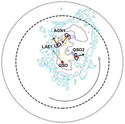
Figure 11: Representation of the spin vectors for the QSO DM halo (gray) and the inspiraling satellites (black with uncertainty range in orange) obtained from the first moment maps of the Ly$\alpha$ and CO(5-4) emissions, respectively. The observed satellite spin vectors are almost aligned with the projected direction to QSO (yellow dashed lines). The inferred spin vector of the DM halo is directed towards the reader with an angle $\eta\approx 40^{\circ}$ (see section 5 for details). For the sake of clarity we indicate with circular arrows indicate the rotation direction for each object. The blue dashed contours show the Ly$\alpha$ emission isophotes as in e.g., Fig 1. The dashed and dotted circle indicates $R_{\rm vir}=163$ kpc or $212$ kpc for the halo mass computed using Moster et al. relations, or Tempel et al. formalism, respectively.

5 Satellites’ spins alignment

Here we discuss, in the framework of the tidal torque theory, the evidence for the alignment between the satellites’ spins and their position vectors to QSO, as reported in section 3.5. The tidal torque theory (Hoyle 1951; Peebles 1969; Doroshkevich 1970; White 1984) is at the basis of the current understanding of galaxies spin acquisition (i.e. angular momentum). In this framework, a net angular momentum is generated in collapsing protogalaxies by tidal torques due to neighbouring perturbations, resulting in a correlation between the galaxy spin direction and the principal axes of the local tidal tensor. Correlations between galaxies spin and large-scale structures (knots, filaments, sheets, voids) are therefore expected in the absence of strong non linear processes. In particular, DM only simulations have shown that halo spins tend to be perpendicular to the closest large-scale filament if their mass is above a critical mass, while low-mass halos are preferentially aligned with the closest filament (e.g., Aragón-Calvo et al. 2007; Codis et al. 2012; Ganeshaiah Veena et al. 2020). This picture also holds for cosmological hydrodynamical simulations that include baryon physics, and feedback processes (e.g., Dubois et al. 2014; Wang et al. 2018), usually showing that galaxies whose stellar mass is $M_{\rm star}\gtrsim 10^{10.5}$ M_⊙ have their spin perpendicular to the closest filament, while lower mass galaxies show a parallel spin (e.g., Codis et al. 2018; Soussana et al. 2020; Kraljic et al. 2020). A consequence of these alignments is that outer satellites (i.e., at $R\gtrsim 0.5R_{\rm vir}$) should show a spin preferentially aligned with their position vector relative to the central object (Welker et al. 2018). In other words, outer low-mass infalling galaxies should have their angular momenta still aligned with the filament they are coming from and parallel to the direction to the central object.

The ELAN here studied, with bright satellites and Ly$\alpha$ emission that reaches the edge of the virial halo, is a perfect laboratory to investigate these theoretical expectations. We first focus on the extended Ly$\alpha$ emission which has been shown to trace the DM halo motions, though with a lag (Arrigoni Battaia et al. 2018a). If we then interpret the Ly$\alpha$ emission as a tracer of halo rotation and that gas and DM spins are almost aligned, the halo spin is likely North-West directed and pointing towards the observer, with an inclination angle $\eta\approx 46^{\circ}$ or $33^{\circ}$ that makes the observed gas circular velocities ($\sim 380$ km s^-1) smaller than the velocities expected for the obtained massive DM halo assuming a NFW profile ($V_{\rm c}^{\rm max}=490$ km s^-1 or $V_{\rm c}^{\rm max}=635$ km s^-1). The fact that we do not detect rotation in the host galaxy of QSO could further suggest that the galaxy spin and inner halo spin are slightly different than the whole halo spin (e.g., Bullock et al. 2001) with the host galaxy spin almost aligned with our line of sight. We note however that strong AGN feedback processes on  10 kpc scales could hinder a weak rotation signal. Secondly, we focus on the satellites (QSO2, AGN1, LAE1) spin alignment with respect to the direction to the central galaxy (QSO). As shown in section 3.5, the three satellites (which all have $M_{\star}<10^{10.5}$ M_⊙) have their major axis defined by the CO(5-4) line of nodes consistent with being perpendicular to the quasar direction. Their spins are therefore almost aligned with the projected position vector to QSO (Table LABEL:tab:Angles). AGN1 is the source with the largest misalignment, possibly due to tidal torques exerted by LAE1, which sits in projected close proximity. AGN1 spin vector is indeed in between the directions to LAE1 and QSO (see cutout in Figure 6). As a last remark, we also notice that AGN1’s spin is anti-aligned with the spins of both LAE1 and QSO2 which are sitting at closer projected distances to QSO.

Overall, all these findings, summarized in Figure 11, are a tentalizing evidence of the theoretical expectations for the angular momentum alignment. The infalling satellites are inspiraling within QSO DM halo with their spins still almost aligned to the large-scale filaments they are coming from, and likely perpendicular to the spin of the QSO DM halo. Follow up observations at a higher spatial resolution (to better resolve the host galaxies and their kinematics; e.g., HST, JWST, and ALMA observations), and at a deeper sensitivity (to detect additional satellites; e.g., MUSE and ALMA observations) are needed to confirm this framework.

6 Ly${\rm\alpha}$ emission versus CO(5-4): signatures of gas infall

In this section we compare the CO(5-4) emission to the Ly$\alpha$ emission in the vicinity of QSO, QSO2, AGN1, and LAE1 to ascertain whether strong radiative transfer effects and/or illumination effects are in place in the vicinity of these sources, ultimately unveiling gas motions for the $T\sim 10^{4}~{}K$ gas. Indeed, while CO(5-4) is a rotational transition which traces well the gas kinematics, the Ly$\alpha$ photons are known to undergo a walk in frequency and space due to resonant scattering in most astrophysical environments (e.g., Neufeld 1990; Laursen et al. 2009a; Dijkstra 2017). Only knowing the systemic redshift of a source allows one to understand the Ly$\alpha$ line shape in the light of emitting gas’ kinematics (e.g., Yang et al. 2011, 2014b, 2014a; Ao et al. 2020). We first discuss the spatial location of the CO(5-4) and Ly$\alpha$ emission, and then compare the line emission shapes.

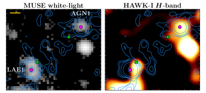
Figure 12: Zoom-in comparison of LAE1 and AGN1 positions in different observations. Left: $9\arcsec\times 7\arcsec$ (or $\sim$68 kpc $\times$ 53 kpc) portion of the MUSE white-light image with highlighted the position of the compact Ly$\alpha$ emission (green crosses) and the position of the CO(5-4) emission (magenta circles) and the ALMA continuum (blue contours; see also Figure 6). The yellow scale in the top-left corner indicates $1\arcsec$. Right: same as the left panel, but for the HAWK-I $H$-band data smoothed with a $1\arcsec$ Gaussian kernel.

As already mentioned in Section 3.5, while for the QSO and QSO2 the location of the 2 mm continuum, CO(5-4) and the Ly$\alpha$ emission coincide, the AGN1 and LAE1 show shifts between the millimeter and the Ly$\alpha$ emission (see Figure 6). Specifically, the centroids of each emission are at distances of 1.5$\arcsec$ (or $\sim 11.4$ kpc) and 0.9$\arcsec$ (or $\sim 6.8$ kpc), respectively for AGN1 and LAE1. For AGN1, a similar shift is found when comparing the location of the Ly$\alpha$ emission and the $H$-band emission from HAWK-I. While for LAE1 the $H$-band emission is in between the Ly$\alpha$ and millimeter emission. We zoom on these shifts in Figure 12. As reported in sections 2.5 and 3.5, our astrometry in the MUSE and HAWK-I data has been checked against GAIA and it is therefore assumed to be correct within small uncertainties. Also, the SMA map shows shifts on the location of its detections especially with respect to MUSE, but we do not consider their positions as well-defined given the low significance of the SMA detections.

The observed shifts between Ly$\alpha$ emission and the infrared continuum could be due to a combination of different effects: (i) presence of a path of least resistance for the Ly$\alpha$ and/or UV photons in these directions (e.g., small scale winds) or dust obscuration (e.g., Hodge et al. 2015), (ii) presence of gas displaced from the host galaxy of LAE1 and AGN1 due to e.g., gas infall, ram pressure or tides, (iii) interaction between two galaxies. A way to disentangle these scenarios is to resolve these systems with high resolution imaging in the UV and NIR wavelength ranges (e.g., HST, JWST) to get their morphologies and inclinations. Another possibility is to compare their CO(5-4) and Ly$\alpha$ line shapes, ultimately constraining the kinematics of the Ly$\alpha$ emitting gas.

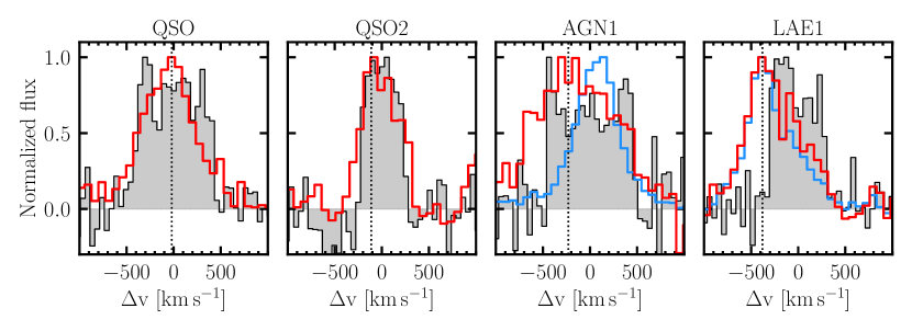
Figure 13: Comparison of the line shapes for CO(5-4) (black-gray) and Ly$\alpha$ emission (red) at the location of QSO, QSO2, AGN1, and LAE1. Zero velocity is the redshift from the CO(5-4) line emission. For AGN1 and LAE1 we also show the Ly$\alpha$ spectrum (blue) at the compact peak in Ly$\alpha$ emission in their vicinity (see section 6; green crosses in Figures 6 and 12). The vertical dotted lines indicate the Ly$\alpha$ velocity shift computed as the first moment of its flux distribution. The ALMA spectra are binned as in Figure 5, while the MUSE data are at the instrument resolution.

Figure 13 shows the comparison of the normalized CO(5-4) line profile (black-gray) together with the normalized Ly$\alpha$ line profile found in the same aperture after continuum subtraction (red) for QSO, QSO2, AGN1 and LAE1. In this figure we use $z_{\rm CO(5-4)}$ as reference velocity (Table LABEL:tab:CO54). The two line profiles clearly differ. The most striking features are (i) the Ly$\alpha$ peak is always blueshifted with respect to the reference velocity of the CO(5-4) line emission, making all Ly$\alpha$ profiles blue-skewed in contrast to most of current observations of high-redshift star-forming galaxies that show a redshifted Ly$\alpha$ with respect to systemic (e.g., Verhamme et al. 2018), (ii) the Ly$\alpha$ blueshift is larger for less massive objects or for smaller SFRs, $\Delta v_{\rm Ly\alpha\ peak}=-20.0\pm 10,-112\pm 7,-250\pm 12,-380\pm 10$ km s^-1, respectively for QSO, QSO2, AGN1, and LAE1, and (iii) an overall similar width for the two emission lines.

All the effects visible in Figure 13 could be easily explained by the radiative transfer of Ly$\alpha$ emission. Indeed, blue-skewed Ly$\alpha$ profiles are expected for infalling gas because photons redward of the line center, that would otherwise escape the medium, are seen in resonance in the reference frame of the infalling atoms, while blue photons easily escape (e.g., Zheng & Miralda-Escudé 2002; Dijkstra et al. 2006a; Verhamme et al. 2006; Laursen et al. 2009a). Specifically, models of Ly$\alpha$ emission from collapsing shells showed that the peak of the resultant Ly$\alpha$ profile depends on the velocity of infall, with the peak progressively displaced towards negative velocities for increasing infall velocities (see e.g., Figure 7 in Verhamme et al. 2006). However, for high enough infall velocities, the peak position is expected to move back closer to line center (i.e., systemic redshift). We argue that the spectra around LAE1, AGN1, QSO2, QSO show this trend, with LAE1 and QSO having respectively the smallest and the largest gas infall velocities in this sample. This can be verified by computing, in first order approximation, the expected infall velocities for these objects. We assume that the gas inflow velocities are constant within the halo, $\sim 0.9v_{\rm vir}$ (e.g., Goerdt & Ceverino 2015), till very close to galaxies (e.g., the aperture for our spectra), with gas then accreting in free-fall onto the galaxies. We also assume as galaxy sizes the observed effective radii of the CO(5-4) emitting regions (Table LABEL:tab:CO54). Integrating the infall velocity formula (e.g., Goerdt & Ceverino 2015) from 14.4 kpc down to the galaxy sizes, we find $v_{\rm inflow}=276,301,310,812$ km s^-1, for LAE1, AGN1, QSO2, and QSO, respectively. Considering also differences in opacities, a factor of $\sim 3$ larger infall velocity for QSO with respect to LAE1 could explain why the Ly$\alpha$ peak near QSO bounces back towards line center because of radiative transfer effects. This would be also in agreement with the expectation of higher accretion rates onto the galaxies with larger SFRs. If the SFR is in steady state with the accretion rate, the inflowing mass at the radius $R$ would be roughly $M_{\rm in}={\rm SFR}/(v_{\rm inflow}/R)$, resulting in about few times $10^{9}$ M_⊙ for each object. We note that such large inflow velocities for cool gas (up to $2\times v_{\rm vir}$) are seen in cosmological simulations of quasar host galaxies in the inner portions of the halo where baryons dominate (Costa et al. 2015).

Instead, the fact that the Ly$\alpha$ and CO(5-4) emissions have similar line widths could be ascribed to resonant scattering effects of Ly$\alpha$ in the presence of dust. Indeed, it has been shown that dust preferentially absorbs Ly$\alpha$ photons in the wings of the line profile because these photons are produced in the dustier regions within galaxies (e.g., Laursen et al. 2009b). Following these predictions, Ly$\alpha$ line profiles in dusty environments should have narrower profiles than in dust-free objects.

Lastly, we checked the Ly$\alpha$ profile also at the location of the bright compact Ly$\alpha$ emission displaced from LAE1 and AGN1, and thanks to which Arrigoni Battaia et al. (2018a) discovered these sources. We show also these spectra (blue) in Figure 13. We have two different configurations. LAE1 presents the same Ly$\alpha$ profile at both locations, i.e. at LAE1 and at $\sim 6.8$ kpc. This implies that we are probing the same infalling material through different sightlines (e.g., Ao et al. 2020). Conversely, AGN1 shows a completely different Ly$\alpha$ profile at $\sim 11.4$ kpc, with its shape slightly red-skewed. This configuration, together with the galaxy kinematics traced by CO(5-4) (section 5) and the fact that He II and C IV emission have been detected at this displaced location (Arrigoni Battaia et al. 2018a) favors a scenario in which we are seeing outflows or material displaced from AGN1 and ionized by its radiation along its minor axis, and inflows along its major axis.

Summarizing, we find signatures of gas infall as traced by Ly$\alpha$ resonant scattering in all of the four sources for which we have a CO(5-4) detection. Detailed resonant scattering calculations are needed to confirm this scenario and test it against contaminations from (i) the large-scale Ly$\alpha$ emission and (ii) the interplay between inflow and outflow signatures within the same observational aperture.

7 Powering of the ELAN

Ly$\alpha$ nebulae around quasars are usually explained by invoking photoionization from the embedded AGN (e.g., Heckman et al. 1991; Weidinger et al. 2005). However, there could be additional powering sources, like star formation in the quasar host galaxy and satellites (e.g., Ao et al. 2015), and/or resonant scattering to large scales of the Ly$\alpha$ photons generated within galaxies/AGN (e.g., Hayes et al. 2011; Geach et al. 2016; Kim et al. 2020), and/or Ly$\alpha$ cooling radiation powered by gravitational collapse (e.g., Haiman et al. 2000; Dijkstra et al. 2006b), and/or fast winds (e.g., Taniguchi & Shioya 2000). In this section we briefly discuss these processes in the framework of the ELAN studied here. The interplay between these mechanisms could be very different in specific systems especially due to geometry (e.g., misalignment between surrounding gas distribution and quasar ionizing cones or quasar obscuration) and the phase in which the system is seen (e.g., ongoing strong wind/outflow or presence of active companions).

Regarding this ELAN, it has been shown that QSO is able to power the entire Ly$\alpha$ emission (${L_{\rm Ly\alpha}^{\rm total}=3.2\times 10^{44}}$ erg s^-1). Specifically, if the whole nebula is within the halo virial radius, the photoionization scenario implies the emitting gas is optically thin to ionizing photons, requiring very high, interstellar-medium densities to explain the absence of He II$\lambda 1640$ down to current observational limits (Arrigoni Battaia et al. 2018a). Cosmological simulations are starting to approach these densities showing ubiquitous cool dense gas throughout the halo of simulated galaxies (e.g., Hummels et al. 2019). Nonetheless, the high densities predicted in a photoionization scenario could be lower if (i) a fraction of the Ly$\alpha$ is due to scattering of photons produced by compact sources, and (ii) star-formation and/or collisional excitation is powering a fraction of the Ly$\alpha$ emission.

We compute a rough estimate for the fraction of Ly$\alpha$ emission powered by star formation by assuming the SFR obtained with CIGALE. We first converted the SFRs to Ly$\alpha$ luminosities assuming (i) case-B recombination, $L_{\rm Ly\alpha}=8.7L_{\rm H\alpha}$ (e.g., Osterbrock & Ferland 2006), and (ii) ${\rm SFR}=7.9\times 10^{-42}L_{\rm H\alpha}$ M_⊙ yr^-1 (e.g., Kennicutt 1998), finding $L_{\rm Ly\alpha}^{\rm QSO}=5.7\times 10^{44}$ erg s^-1, $L_{\rm Ly\alpha}^{\rm QSO2}=2.0\times 10^{44}$ erg s^-1, $L_{\rm Ly\alpha}^{\rm AGN1}=1.1\times 10^{44}$ erg s^-1, $L_{\rm Ly\alpha}^{\rm LAE1}=5.5\times 10^{43}$ erg s^-1. The sum of these values clearly exceed the total observed Ly$\alpha$ emission for the ELAN. However, this calculation assumes that all ionizing photons impinge on the gas. This is likely not the case as it has been shown that the average escape fraction at similar redshifts is $\sim 5\%$ (e.g., Matthee et al. 2017). Assuming this escape fraction, the total SFR of the four objects could therefore power only $\sim 14\%$ of the observed Ly$\alpha$ emission. At a fixed cool gas mass, this contribution would lower the predicted $n_{\rm H}$ from recombination by a similar amount.

On top of this, a comparable fraction of Ly$\alpha$ photons produced in the body of galaxies due to SFR and/or AGN could escape and thus scatter in the surrounding gas distribution and eventually escape towards the observer (e.g., Duval et al. 2014). Because of the absence of compact Ly$\alpha$ emission at the location of the ALMA continuum for LAE1 and AGN1, we think that the escape of Ly$\alpha$ photons and/or UV photons from these objects is highly directional. Indeed we find that the displaced compact Ly$\alpha$ emission in close vicinity to the location of LAE1 and AGN1 (see section 6; Arrigoni Battaia et al. 2018a) corresponds to $8.7\%$ and $7.7\%$ of their Ly$\alpha$ emission expected from SFR, respectively. These values might represent an upper limit on the fraction of Ly$\alpha$ photons scattered outside each galaxy. Therefore, this calculation suggests that all the compact sources within the ELAN may contribute up to at least $\sim 30\%$ considering both photoionization from SFR and resonant scattering.

We can further compute a conservative estimate for the Ly$\alpha$ photons available for scattering and produced by the QSO. To this aim, the Ly$\alpha$ line is convolved with the line shape of the observed ELAN, and integrated to obtained $(L_{\rm Ly\alpha}^{\rm QSO})_{\rm obs}=6.4\times 10^{44}$ erg s^-1, which is $\sim 2\times$ the total ELAN luminosity. As also QSO photons outside of this range can in principle interact with the ELAN gas after some scattering, the available QSO Ly$\alpha$ photons abundantly pass the total Ly$\alpha$ luminosity of the ELAN. Nevertheless, because of the physics inherent to the propagation of resonant scattering photons (e.g., Dijkstra 2017) and because of the large distances within the halo, scattered QSO photons likely dominate the nebula powering preferentially in the inner halo (see discussion in Arrigoni Battaia et al. 2018a and references therein).

In addition, a fraction of the Ly$\alpha$ emission in this massive system could be due to collisional excitation (e.g., Furlanetto et al. 2005). This contribution is notoriously difficult to predict as it strongly depends on temperature (exponential dependence) and gas density squared (Osterbrock 1989). Analytical and numerical studies considering this powering mechanism did reproduce the observed Ly$\alpha$ luminosities of high-redshift nebulae, underlying the possible importance of this mechanism (Dijkstra & Loeb 2009; Rosdahl & Blaizot 2012). For example, cosmological simulations of structure formation for massive halos showed that the Ly$\alpha$ emission from the gas with $n_{\rm H}\gtrsim 0.3$ cm^-3 (the cool halo gas for those simulations) is dominated by collisional excitation and accounts for 40% of the total luminosity (Rosdahl & Blaizot 2012). These simulations did not include AGN photoionization and therefore their results need to be taken with caution when compared to the system studied here.

Lastly, given the active nature (both AGN and SFR) of the sources within the ELAN, fast winds or even outflows are expected to be present at some times during its evolution. Fast shocks generated in this scenario would produce a strong ultraviolet radiation field (e.g., Allen et al. 2008), which can contribute to the powering of the ELAN. Arrigoni Battaia et al. (2018a) discussed how the $300$ kpc velocity shear and small Ly$\alpha$ velocity dispersion across this ELAN run counter to the presence of an halo-scale wind. However, small scales ($\sim 10$ kpc) winds in proximity of the compact sources within the ELAN could not be excluded. Our observations seem to confirm this picture, showing possible evidence for winds around at least AGN1 (section 6). A certain portion of the ELAN could be therefore powered by such small-scales winds.

Overall, a complex interplay between AGN and SFR ionization, Ly$\alpha$ resonant scattering, fast winds, and collisional excitation is needed to fully comprehend the powering of ELANe. Their large and often asymmetric extents are likely due to the presence of active companions which help in illuminating the surrounding gas distribution. Similar conclusions have been reported when studying the widespread Ly$\alpha$ emission in a $z\sim 3$ protocluster field (Umehata et al. 2019).

8 Note on molecular gas extending outside the body of galaxies

Widespread large reservoirs ($\sim 10^{11}$ M_⊙) of cold molecular gas have been found across $\sim 40-70$ kpc in two $z\sim 2$ HzRGs fields. In one case the reservoir was found in proximity of the HzRG itself (Emonts et al. 2016, 2018), while in the second case around an H$\alpha$ emitter (Dannerbauer et al. 2017). Because of the similarities between the ELAN studied here and the halo expected to host an HzRG, and the high densities usually invoked to explain the Ly$\alpha$ emission, it is possible that ELANe are multiphasic, at least on tens of kpc close to embedded sources (see also Vidal-García et al. 2021). Interestingly, an extended molecular gas reservoir as massive as those found in HzRGs would increase the molecular gas budget for the targeted ELAN to values similar to the stars budget (see Fig. 10). We note that this occurrence is within our current conservative error estimate for the molecular phase.

The CO(5-4) ALMA observations presented in section 3.5 provide sizes for the CO(5-4) emitting region for QSO, QSO2, AGN1 and LAE1 in the range $R_{\rm CO(5-4)}\sim 3-5$ kpc. These values are in overall agreement with current molecular sizes reported for different high-redshift galaxy populations (e.g., SMGs, Ivison et al. 2011; Spilker et al. 2015; Chen et al. 2017; Calistro Rivera et al. 2018; quasars, Decarli et al. 2018; Stacey et al. 2020; HzRG disks, Man et al. 2019; star-forming galaxies, Kaasinen et al. 2020), but possibly on the high-side, especially for QSO2 and AGN1. However, there are no statistical observations of CO(5-4) sizes in high-redshift objects, nor many CO size estimates at $z\sim 3$, hampering any firm conclusion.

Nevertheless, the ALMA observations did not unveil any large-scale, widespread molecular reservoir in the system studied here. Assuming that the excitation in a hypothetical extended molecular reservoir is similar to within the compact sources ($r_{51}=0.4$, $\alpha_{\rm CO}=0.8$ M_⊙ (K km s^-1 pc^-2)^-1), and considering a line width of $\sim 300$ km s^-1, 3$\times$ the noise rms ($\approx 167$ $\mu$Jy) corresponds to a molecular gass limit $3.4\times 10^{8}$ M_⊙ beam^-1, which implies a beam-averaged surface molecular gas mass $\Sigma_{\rm H2}<19$ M_⊙ pc². This value is consistent with similar non detections in other two ELANe (Decarli et al. 2021), excluding molecular gas surface densities similar to starbursting environment in the whole extent of the ELAN. We further checked our data by applying a taper, up to considering only the range of uv-distances sensitive to scales $\sim 12-30$ arcsec. These tapered data have a noise ${\rm rms}\sim 594$ $\mu$Jy beam^-1 in $\sim 50$ km s^-1. Again, we did not find any detection (corresponding to a beam-averaged surface molecular gas mass $3\sigma$ limit of $\Sigma_{\rm H2}<69$ M_⊙ pc²), confirming that CO(5-4) traces excited molecular gas within the body of galaxies. Deeper observations of ELAN systems targeting low-J CO transitions or additional molecular gas tracers (e.g., [CI] and [CII] emission) are therefore needed to unveil the extended molecular gas reservoir, if any exists.

9 Summary

We initiated the project “a multiwavelength study of ELAN environments” (AMUSE²) to investigate several aspects of the astrophysics of high-redshift massive systems associated with quasars, which ELANe seem to trace. In this paper, we report on VLT/HAWK-I, APEX/LABOCA, JCMT/SCUBA-2, SMA/850$\mu$m, ALMA/CO(5-4) and 2mm observations targeting the ELAN around the $z\sim 3$ quasar SDSSJ 1040+1020 (a.k.a QSO) discovered by Arrigoni Battaia et al. (2018a). This ELAN was known to host three AGN and two LAEs (LAE1 and LAE2). Specifically, VLT/MUSE unveiled that the bright central quasar QSO has a companion quasar QSO2 and a companion type-II AGN, AGN1.

The single dish observations resulted in a surprisingly strong detection at 850 $\mu$m ($\sim 11$ mJy) at the ELAN location. However, the interferometric observations confirmed that this emission accounts for multiple sources associated with the ELAN. Our multiwavelength observations added several continuum data-points to the four brightest sources SED (QSO, QSO2, AGN1, LAE1), and unveiled their relatively boxy CO(5-4) emission with integrated flux in the range $0.22\lesssim I_{\rm CO(5-4)}\lesssim 0.43$ Jy km s^-1. This emission is spatially resolved and shows evidence of kinematics reminiscent of rotation-like patterns in three sources, QSO2, AGN1, and LAE1. Further, the Ly$\alpha$ emission in the vicinity of AGN1 and LAE1 is found to peak at a displaced position with respect to the continuua and the CO(5-4) emission, by $\sim 11.4$ kpc and $\sim 6.8$ kpc, respectively. A comparison of the Ly$\alpha$ emission extracted from the same aperture of the CO(5-4) emission revealed blue-skewed Ly$\alpha$ spectra for all four sources, and comparable line widths.

We use this dataset to attempt a first calculation of the total mass of the system and forecast its evolution. First, stellar and dust masses, and star formation rates are obtained through SED fitting for the sources with confirmed association, i.e., QSO, QSO2, AGN1, and LAE1. While their molecular gas masses are obtained from the CO(5-4) detections. The estimated stellar, dust, and molecular gas masses are consistent with the dynamical masses obtained from CO(5-4) under the assumption of a reasonable inclination angle. Further, two orthogonal methods are used to infer the total DM halo mass hosting this ELAN system: the halo mass - stellar mass relation, and the use of radial velocity dispersion and group extent. Both methods give a consistent answer, this ELAN likely inhabits a massive DM halo of M${}_{\rm DM}=(0.8-2)\times 10^{13}$ M_⊙. Following this methodology, our main findings are as follows.

1. The total current SFR in the system is at least SFR $\sim 860$ M_⊙ yr^-1, with the QSO host being the most star-forming galaxy SFR$\sim 500$ M_⊙ yr^-1 (section 4.1).

2. The molecular gas mass estimated through the CO(5-4) emission for QSO, QSO2, AGN1 and LAE1 is $M_{\rm H_{2}}\sim 10^{10}$ M_⊙ for each system. The dust content in these galaxies is found to be in the range $M_{\rm dust}=(0.3-4)\times 10^{9}$ M_⊙ (Table LABEL:tab:CO54; section 4).

3. The total baryonic mass budget for the whole system considering the stellar, dust, molecular, cool gas ($T\sim 10^{4}$ K), and cold gas ($T\sim 100$ K) masses, sums up to $10-21$% of the cosmic baryon fraction. Therefore a hot reservoir as massive as $M_{\rm warm-hot}\sim 10^{12}$ M_⊙ is needed to complete the cosmic baryon budget for such a halo. Assuming baryon fractions seen in current cosmological simulations (i.e., $\sim 1/3$ of the cosmic value), the hot phase would instead represent $74-88$% of the baryons in this system (section 4.4).

4. The fate of the system is predicted by estimating the molecular depletion time scale for each object and considering its halo mass and expected mass accretion rates. The targeted ELAN is likely the progenitor of an elliptical galaxy as massive as giant local ellipticals (e.g., NGC 4365, NGC 5044), and with its DM halo expected to achieve by $z=0$ a DM mass as high as $10^{14.7}$ M_⊙ (section 4.5).

The observations further probe several aspects of the interplay between the galaxies embedded in the ELAN and the large-scale gas distribution. The main points we discussed are as follows.

1. The first-moment maps of the CO(5-4) emission show rotation signatures in QSO2, AGN1, and LAE1. Their projected angular momentum vectors, though uncertain, are found to be almost parallel to the projected position vector to the central QSO. This finding hints to a scenario in which the infalling QSO satellites have their spins still almost aligned to the large-scale filaments they come from. Further, the spin of the QSO DM halo, inferred by assuming that the Ly$\alpha$ signal traces halo motions with a certain lag (Arrigoni Battaia et al. 2018a), is roughly perpendicular to those of the satellites. These results would be in line with the theoretical expectations from the tidal torque theory (section 5).

2. Tentalizing signatures of gas infall onto QSO, QSO2, AGN1, LAE1 are evident when comparing the Ly$\alpha$ emission shape with respect to the redshift obtained from the CO(5-4) emission. Indeed, the observed line shapes could be explained by Ly$\alpha$ radiative transfer effects in infalling gas in dusty environments. Further, the velocity shifts of the Ly$\alpha$ peaks decrease with increasing stellar mass or SFR, with QSO (LAE1) having the smallest (largest) negative shift in the sample of four sources. This effect could be due to higher infall velocities onto more massive systems, with the infall velocities onto the QSO host galaxy being the largest. This picture agrees with the SFRs in these systems, i.e. highest (lowest) SFR in QSO (LAE1) (section 6).

3. Additional likely signatures of Ly$\alpha$ resonant scattering are the large displacements ($\sim 10$ kpc) of the peak emission around LAE1 and AGN1 with respect to their ALMA and HAWK-I detections. Resonant scattering of Ly$\alpha$ photons seems therefore in place around each source on scales as large as 10-15 kpc (section 6).

4. SFR and Ly$\alpha$ resonant scattering from all the compact sources within the ELAN may contribute up to at least $\sim 30$% of the total luminosity of the ELAN, with the fraction of Ly$\alpha$ scattered photons from the quasar being a large incognita. Future radiative transfer calculations with high-resolution cosmological simulations of similar massive systems may shed light on the powering of ELANe (section 7).

5. No large-scale molecular reservoir is found as traced by CO(5-4) down to $\Sigma_{H2}<19$ M_⊙ pc², confirming that high $J$-transitions trace highly excited CO gas on kiloparsecs scales (section 8). Observations at lower $J$ transitions or additional tracers are needed to unveil extended molecular reservoirs in ELANe (if any).

Overall these observations confirm the richness of information encoded in ELAN systems. These rare objects can be used as laboratories to study several open questions regarding the high redshift universe, from the angular momentum accretion onto galaxies, to gas infall from large-scales to quasar scales, to the cool gas phase and its coexistence with a warm-hot phase. Current and future top-notch facilities (e.g., BlueMUSE, Richard et al. 2019; JWST, Gardner et al. 2006) will allow us to address in increasing details the astrophysics of these massive systems, and ultimately pin down the physics regulating their baryons flow and galaxy evolution.

Appendix A The APEX/LABOCA and JCMT/SCUBA-2 maps

In this appendix we show, for completeness, the APEX/LABOCA and JCMT/SCUBA-2 maps for the full area covered by the observations (Figures 14,15). In this work we focus only on the ELAN location (the black box in each map) and we defer to an other paper of this series (Nowotka et al. 2021) the characterization of the ELAN large-scale environment (e.g., Arrigoni Battaia et al. 2018b).

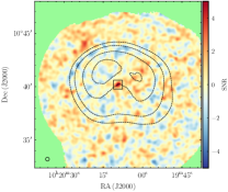
Figure 14: 870 $\mu$m LABOCA S/N map of the field around the ELAN. Dashed contours indicate the noise at 4.0, 3.5, 3.0, and 2.7 mJy beam^-1, from the outer to the inner portion of the map. The black box shows the location of the ELAN and has the size of the cutout shown in Figure 1. The region within a noise of 4 mJy beam^-1 represents a field of 68 arcmin² (or $\sim 14$ Mpc²). In the green region there are no data. The main beam of LABOCA is shown in the bottom left corner.

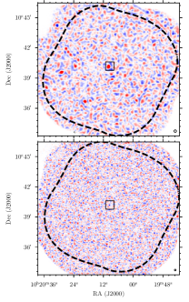
Figure 15: SCUBA-2 S/N maps at $850$ $\mu$m (top panel) and $450$ $\mu$m (bottom panel) for the field around the ELAN. The black square indicates the field of view of Figure 1. The maps are shown with a linear scale from -5 (blue) to 5 (red). For both fields, we indicate the noise contour (black dashed) for 3$\times$ the central noise and the effective beam of the observations in the bottom right corner.

Appendix B Flux deboosting for JCMT/SCUBA-2 and APEX/LABOCA observations

The flux densities of detections at low S/N in sub-millimeter observations are usually boosted due to the presence of noise fluctuations (e.g., Eales et al. 2000; Coppin et al. 2006; Simpson et al. 2015). We quantify the flux boosting affecting the SCUBA-2 and LABOCA data by comparing the fluxes of injected mock sources with their recovered fluxes. Specifically, we proceed as follows. First, we created jackknife maps by inverting half of the scans during the coadding, keeping all processing steps as for the normal data reduction. Being thus free of any astronomical signal, these jackknife maps serve as noise maps. For each instrument, we then created 1500 mock maps by injecting sources in the respective jackknife map, assuming a broken power-law for the counts with parameter values as in Arrigoni Battaia et al. (2018b). We then extracted the mock sources with a similar algorithm as in Section 3.2, but using the psf of the 850$\mu$m/SCUBA-2 (e.g., Chen et al. 2013b) and LABOCA (e.g., Weiß et al. 2009) instruments. Figure 16, and 17 show the results for SCUBA-2 and LABOCA, respectively. We note that we have a much larger number of detected sources in the SCUBA-2 850 $\mu$m maps because of their better sensitivity.

At the S/N of the detected emission at the ELAN position we found an average flux boosting of 1.09 and 1.19, respectively for SCUBA-2 and LABOCA. These values are in agreement within uncertainties with previous estimates of flux boosting for these instruments, 1.05 (Chen et al. 2013a) and 1.13 (Weiß et al. 2009), respectively for SCUBA-2 at 850 $\mu$m and LABOCA. We use the found average values to correct for this effect (Table LABEL:tab:SingleDish).

Figure 16: The ratio between the output and the input flux densities of mock sources as a function of the input S/N for the SCUBA-2 850 $\mu$m observations. The data-points obtained from 1500 realizations are shown in 2D hexagonal bins (high density of points in blue; low density in brown). We show the mean (red) and the median (yellow) values of the flux ratio. The blue dashed curves enclose the $1\sigma$ range relative to the mean curve. To help guiding the eye, the cyan line indicates the ratio $f_{\rm out}/f_{\rm in}=1$. In this work we correct the flux densitiy of the detected source at the ELAN position using the mean curve (see Table LABEL:tab:SingleDish).

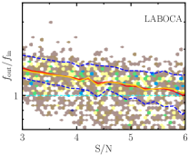
Figure 17: The ratio between the output and the input flux densities of mock sources as a function of the input S/N for the LABOCA observations. The data-points obtained from 1500 realizations are shown in 2D hexagonal bins (high density of points in blue; low density in brown). We show the mean (red) and the median (yellow) values of the flux ratio. The blue dashed curves enclose the $1\sigma$ range relative to the mean curve. To help guiding the eye, the cyan line indicates the ratio $f_{\rm out}/f_{\rm in}=1$. In this work we correct the flux densities of the detected source at the ELAN position using the mean curve (see Table LABEL:tab:SingleDish).

Appendix C Flux deboosting for SMA continuum sources

To quantify the level of flux boosting in the SMA data we proceeded as follows. First, we constructed a Jackknife map, i.e., a noise map, as described in Section 2.3. We then created 5000 SMA observations by injecting in each map 10 mock point sources with uniformly distributed random fluxes between 1 and 10 times the noise level. The sources are introduced at random locations within an area equal to the primary beam of the SMA observations. We then extracted sources from these 5000 realizations by using the same algorithm used for the detection of sources in Section 3.2. A source is considered to be recovered if it is detected with S/N$\geq 2$ and within one beam width from the position of injection. The recovered and input flux densities are then compared to constrain the flux boosting at different input S/N. Figure 18 shows the results of this comparison. Sources with input S/N$=2$ (5) are boosted on average (red curve) by 84% (20%), while the flux boosting is only about 10% for sources at S/N$>7$. We corrected the flux densities in our SMA catalogue based on the average curve shown in Figure 18.

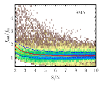
Figure 18: The ratio between the output and the input flux densities of mock sources as a function of the input S/N for the SMA observations. The data-points obtained from 5000 realizations are shown in 2D hexagonal bins (high density of points in blue; low density in brown). We show the mean (red) and the median (yellow) values of the flux ratio. The blue dashed curves enclose the $1\sigma$ range relative to the mean curve. To help guiding the eye, the cyan line indicates the ratio $f_{\rm out}/f_{\rm in}=1$. In this work we correct the flux densities of the detected sources using the mean curve (see Table LABEL:tab:Interf).

Appendix D Flux deboosting for ALMA continuum sources

We quantify the flux boosting for the ALMA data following exactly the same approach as for the SMA data, though using the algorithm for detection outlined in Section 3.3, and the noise map obtained in Section 2.4. Figure 19 shows the ratio between the recovered and input flux densities. We find that sources with input S/N$=4$ are boosted on average (red curve) by 17%, while the flux boosting becomes negligible for sources with S/N$>10$. We used the average curve shown in Figure 19 to correct the flux densities in our ALMA catalogue. We note that similar corrections are found in the literature in number counts studies conducted with ALMA, though at different wavelengths (e.g., Simpson et al. 2015; Oteo et al. 2016).

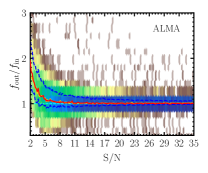
Figure 19: The ratio between the output and the input flux densities of mock sources as a function of the input S/N for the ALMA continuum observations. The data-points obtained from 5000 realizations are shown in 2D hexagonal bins (high density of points in blue; low density in brown). We show the mean (red) and the median (yellow) values of the flux ratio. The blue dashed curves enclose the $1\sigma$ range relative to the mean curve. To help guiding the eye, the cyan line indicates the ratio $f_{\rm out}/f_{\rm in}=1$. In this work we correct the flux densities of the detected sources using the mean curve (see Table LABEL:tab:Interf).

Appendix E Data-points for the spectral energy distributions of CO(5-4) detected sources

In table LABEL:tab:app_phot we list for completeness the photometric data obtained from the literature and used in the SED fitting for QSO, QSO2, AGN1, and LAE1.

Table 5: Data obtained from the literature for the SED fitting of QSO, QSO2, AGN1, and LAE1 (all units in mJy)^a.

ID	$J$	$H$	$K_{s}$	W1	W2	W3	W4	1.4 GHz
QSO	$0.35\pm 0.05$	$0.66\pm 0.07$	$0.50\pm 0.08$	$0.60\pm 0.02$	$0.68\pm 0.02$	$2.47\pm 0.14$	$4.70\pm 0.86$	$<0.4$
QSO2	-	-	-	$<0.04$	$<0.09$	$<0.7$	$<6.9$	$<0.4$
AGN1	-	-	-	$<0.04$	$<0.09$	$<0.7$	$<6.9$	$<0.4$
LAE1	-	-	-	$<0.04$	$<0.09$	$<0.7$	$<6.9$	$<0.4$

References

- Alam et al. (2015) Alam, S., Albareti, F. D., Allende Prieto, C., et al. 2015, ApJS, 219, 12, doi: 10.1088/0067-0049/219/1/12
- Allen et al. (2008) Allen, M. G., Groves, B. A., Dopita, M. A., Sutherland, R. S., & Kewley, L. J. 2008, ApJS, 178, 20, doi: 10.1086/589652
- Ao et al. (2015) Ao, Y., Matsuda, Y., Beelen, A., et al. 2015, A&A, 581, A132, doi: 10.1051/0004-6361/201424165
- Ao et al. (2020) Ao, Y., Zheng, Z., Henkel, C., et al. 2020, Nature Astronomy, 4, 670, doi: 10.1038/s41550-020-1033-3
- Aragón-Calvo et al. (2007) Aragón-Calvo, M. A., van de Weygaert, R., Jones, B. J. T., & van der Hulst, J. M. 2007, ApJ, 655, L5, doi: 10.1086/511633
- Aravena et al. (2019) Aravena, M., Decarli, R., Gónzalez-López, J., et al. 2019, ApJ, 882, 136, doi: 10.3847/1538-4357/ab30df
- Archibald et al. (2001) Archibald, E. N., Dunlop, J. S., Hughes, D. H., et al. 2001, MNRAS, 323, 417, doi: 10.1046/j.1365-8711.2001.04188.x
- Arrigoni Battaia et al. (2016) Arrigoni Battaia, F., Hennawi, J. F., Cantalupo, S., & Prochaska, J. X. 2016, ApJ, 829, 3, doi: 10.3847/0004-637X/829/1/3
- Arrigoni Battaia et al. (2015a) Arrigoni Battaia, F., Hennawi, J. F., Prochaska, J. X., & Cantalupo, S. 2015a, ApJ, 809, 163, doi: 10.1088/0004-637X/809/2/163
- Arrigoni Battaia et al. (2019) Arrigoni Battaia, F., Hennawi, J. F., Prochaska, J. X., et al. 2019, MNRAS, 482, 3162, doi: 10.1093/mnras/sty2827
- Arrigoni Battaia et al. (2018a) Arrigoni Battaia, F., Prochaska, J. X., Hennawi, J. F., et al. 2018a, MNRAS, 473, 3907, doi: 10.1093/mnras/stx2465
- Arrigoni Battaia et al. (2015b) Arrigoni Battaia, F., Yang, Y., Hennawi, J. F., et al. 2015b, ApJ, 804, 26, doi: 10.1088/0004-637X/804/1/26
- Arrigoni Battaia et al. (2018b) Arrigoni Battaia, F., Chen, C.-C., Fumagalli, M., et al. 2018b, A&A, 620, A202, doi: 10.1051/0004-6361/201834195
- Astropy Collaboration et al. (2013) Astropy Collaboration, Robitaille, T. P., Tollerud, E. J., et al. 2013, A&A, 558, A33, doi: 10.1051/0004-6361/201322068
- Astropy Collaboration et al. (2018) Astropy Collaboration, Price-Whelan, A. M., Sipőcz, B. M., et al. 2018, AJ, 156, 123, doi: 10.3847/1538-3881/aabc4f
- Bacon et al. (2010) Bacon, R., Accardo, M., Adjali, L., et al. 2010, in Society of Photo-Optical Instrumentation Engineers (SPIE) Conference Series, Vol. 7735, Society of Photo-Optical Instrumentation Engineers (SPIE) Conference Series, doi: 10.1117/12.856027
- Balashev et al. (2017) Balashev, S. A., Noterdaeme, P., Rahmani, H., et al. 2017, MNRAS, 470, 2890, doi: 10.1093/mnras/stx1339
- Barvainis et al. (1997) Barvainis, R., Maloney, P., Antonucci, R., & Alloin, D. 1997, ApJ, 484, 695, doi: 10.1086/304382
- Becker et al. (1994) Becker, R. H., White, R. L., & Helfand, D. J. 1994, in Astronomical Society of the Pacific Conference Series, Vol. 61, Astronomical Data Analysis Software and Systems III, ed. D. R. Crabtree, R. J. Hanisch, & J. Barnes, 165
- Beelen et al. (2006) Beelen, A., Cox, P., Benford, D. J., et al. 2006, ApJ, 642, 694, doi: 10.1086/500636
- Binney & Tremaine (2008) Binney, J., & Tremaine, S. 2008, Galactic Dynamics: Second Edition
- Birkin et al. (2020) Birkin, J. E., Weiss, A., Wardlow, J. L., et al. 2020, arXiv e-prints, arXiv:2009.03341. https://arxiv.org/abs/2009.03341
- Birkin et al. (2021) —. 2021, MNRAS, 501, 3926, doi: 10.1093/mnras/staa3862
- Bischetti et al. (2021) Bischetti, M., Feruglio, C., Piconcelli, E., et al. 2021, A&A, 645, A33, doi: 10.1051/0004-6361/202039057
- Bolatto et al. (2013) Bolatto, A. D., Wolfire, M., & Leroy, A. K. 2013, ARA&A, 51, 207, doi: 10.1146/annurev-astro-082812-140944
- Boogaard et al. (2020) Boogaard, L. A., van der Werf, P., Weiss, A., et al. 2020, ApJ, 902, 109, doi: 10.3847/1538-4357/abb82f
- Boquien et al. (2019) Boquien, M., Burgarella, D., Roehlly, Y., et al. 2019, A&A, 622, A103, doi: 10.1051/0004-6361/201834156
- Borisova et al. (2016) Borisova, E., Cantalupo, S., Lilly, S. J., et al. 2016, ApJ, 831, 39, doi: 10.3847/0004-637X/831/1/39
- Bothwell et al. (2013) Bothwell, M. S., Smail, I., Chapman, S. C., et al. 2013, MNRAS, 429, 3047, doi: 10.1093/mnras/sts562
- Bruzual & Charlot (2003) Bruzual, G., & Charlot, S. 2003, MNRAS, 344, 1000, doi: 10.1046/j.1365-8711.2003.06897.x
- Bădescu et al. (2017) Bădescu, T., Yang, Y., Bertoldi, F., et al. 2017, ApJ, 845, 172, doi: 10.3847/1538-4357/aa8220
- Bullock et al. (2001) Bullock, J. S., Dekel, A., Kolatt, T. S., et al. 2001, ApJ, 555, 240, doi: 10.1086/321477
- Cai et al. (2017) Cai, Z., Fan, X., Yang, Y., et al. 2017, ApJ, 837, 71, doi: 10.3847/1538-4357/aa5d14
- Cai et al. (2019) Cai, Z., Cantalupo, S., Prochaska, J. X., et al. 2019, ApJS, 245, 23, doi: 10.3847/1538-4365/ab4796
- Calistro Rivera et al. (2016) Calistro Rivera, G., Lusso, E., Hennawi, J. F., & Hogg, D. W. 2016, ApJ, 833, 98, doi: 10.3847/1538-4357/833/1/98
- Calistro Rivera et al. (2018) Calistro Rivera, G., Hodge, J. A., Smail, I., et al. 2018, ApJ, 863, 56, doi: 10.3847/1538-4357/aacffa
- Calzetti et al. (2000) Calzetti, D., Armus, L., Bohlin, R. C., et al. 2000, ApJ, 533, 682, doi: 10.1086/308692
- Cantalupo et al. (2014) Cantalupo, S., Arrigoni-Battaia, F., Prochaska, J. X., Hennawi, J. F., & Madau, P. 2014, Nature, 506, 63, doi: 10.1038/nature12898
- Carilli & Walter (2013) Carilli, C. L., & Walter, F. 2013, ARA&A, 51, 105, doi: 10.1146/annurev-astro-082812-140953
- Carilli et al. (2007) Carilli, C. L., Neri, R., Wang, R., et al. 2007, ApJ, 666, L9, doi: 10.1086/521648
- Casali et al. (2006) Casali, M., Pirard, J.-F., Kissler-Patig, M., et al. 2006, in Society of Photo-Optical Instrumentation Engineers (SPIE) Conference Series, Vol. 6269, Proc. SPIE, 62690W, doi: 10.1117/12.670150
- Casey et al. (2014) Casey, C. M., Narayanan, D., & Cooray, A. 2014, Phys. Rep., 541, 45, doi: 10.1016/j.physrep.2014.02.009
- Chabrier (2003) Chabrier, G. 2003, PASP, 115, 763, doi: 10.1086/376392
- Chapin et al. (2013) Chapin, E. L., Berry, D. S., Gibb, A. G., et al. 2013, MNRAS, 430, 2545, doi: 10.1093/mnras/stt052
- Chen et al. (2013a) Chen, C.-C., Cowie, L. L., Barger, A. J., et al. 2013a, ApJ, 762, 81, doi: 10.1088/0004-637X/762/2/81
- Chen et al. (2013b) —. 2013b, ApJ, 776, 131, doi: 10.1088/0004-637X/776/2/131
- Chen et al. (2017) Chen, C.-C., Hodge, J. A., Smail, I., et al. 2017, ApJ, 846, 108, doi: 10.3847/1538-4357/aa863a
- Chevance et al. (2020) Chevance, M., Kruijssen, J. M. D., Vazquez-Semadeni, E., et al. 2020, Space Sci. Rev., 216, 50, doi: 10.1007/s11214-020-00674-x
- Chiang et al. (2013) Chiang, Y.-K., Overzier, R., & Gebhardt, K. 2013, ApJ, 779, 127, doi: 10.1088/0004-637X/779/2/127
- Circosta et al. (2018) Circosta, C., Mainieri, V., Padovani, P., et al. 2018, A&A, 620, A82, doi: 10.1051/0004-6361/201833520
- Codis et al. (2018) Codis, S., Jindal, A., Chisari, N. E., et al. 2018, MNRAS, 481, 4753, doi: 10.1093/mnras/sty2567
- Codis et al. (2012) Codis, S., Pichon, C., Devriendt, J., et al. 2012, MNRAS, 427, 3320, doi: 10.1111/j.1365-2966.2012.21636.x
- Coppin et al. (2006) Coppin, K., Chapin, E. L., Mortier, A. M. J., et al. 2006, MNRAS, 372, 1621, doi: 10.1111/j.1365-2966.2006.10961.x
- Coppin et al. (2008) Coppin, K. E. K., Swinbank, A. M., Neri, R., et al. 2008, MNRAS, 389, 45, doi: 10.1111/j.1365-2966.2008.13553.x
- Correa et al. (2018) Correa, C. A., Schaye, J., Wyithe, J. S. B., et al. 2018, MNRAS, 473, 538, doi: 10.1093/mnras/stx2332
- Cortzen et al. (2020) Cortzen, I., Magdis, G. E., Valentino, F., et al. 2020, A&A, 634, L14, doi: 10.1051/0004-6361/201937217
- Costa et al. (2015) Costa, T., Sijacki, D., & Haehnelt, M. G. 2015, MNRAS, 448, L30, doi: 10.1093/mnrasl/slu193
- Courteau (1997) Courteau, S. 1997, AJ, 114, 2402, doi: 10.1086/118656
- Cowie et al. (2017) Cowie, L. L., Barger, A. J., Hsu, L. Y., et al. 2017, ApJ, 837, 139, doi: 10.3847/1538-4357/aa60bb
- da Cunha et al. (2015) da Cunha, E., Walter, F., Smail, I. R., et al. 2015, ApJ, 806, 110, doi: 10.1088/0004-637X/806/1/110
- Daddi et al. (2015) Daddi, E., Dannerbauer, H., Liu, D., et al. 2015, A&A, 577, A46, doi: 10.1051/0004-6361/201425043
- Dannerbauer et al. (2017) Dannerbauer, H., Lehnert, M. D., Emonts, B., et al. 2017, A&A, 608, A48, doi: 10.1051/0004-6361/201730449
- Davé (2009) Davé, R. 2009, in Astronomical Society of the Pacific Conference Series, Vol. 419, Galaxy Evolution: Emerging Insights and Future Challenges, ed. S. Jogee, I. Marinova, L. Hao, & G. A. Blanc, 347. https://arxiv.org/abs/0901.3149
- De Breuck et al. (2010) De Breuck, C., Seymour, N., Stern, D., et al. 2010, ApJ, 725, 36, doi: 10.1088/0004-637X/725/1/36
- Decarli et al. (2021) Decarli, R., Arrigoni-Battaia, F., Hennawi, J. F., et al. 2021, A&A, 645, L3, doi: 10.1051/0004-6361/202039814
- Decarli et al. (2010) Decarli, R., Falomo, R., Treves, A., et al. 2010, MNRAS, 402, 2441, doi: 10.1111/j.1365-2966.2009.16048.x
- Decarli et al. (2018) Decarli, R., Walter, F., Venemans, B. P., et al. 2018, ApJ, 854, 97, doi: 10.3847/1538-4357/aaa5aa
- Dekel & Birnboim (2006) Dekel, A., & Birnboim, Y. 2006, MNRAS, 368, 2, doi: 10.1111/j.1365-2966.2006.10145.x
- Dempsey et al. (2013) Dempsey, J. T., Friberg, P., Jenness, T., et al. 2013, MNRAS, 430, 2534, doi: 10.1093/mnras/stt090
- Dijkstra (2017) Dijkstra, M. 2017, ArXiv e-prints. https://arxiv.org/abs/1704.03416
- Dijkstra et al. (2006a) Dijkstra, M., Haiman, Z., & Spaans, M. 2006a, ApJ, 649, 14, doi: 10.1086/506243
- Dijkstra et al. (2006b) —. 2006b, ApJ, 649, 37, doi: 10.1086/506244
- Dijkstra & Loeb (2009) Dijkstra, M., & Loeb, A. 2009, MNRAS, 400, 1109, doi: 10.1111/j.1365-2966.2009.15533.x
- Donevski et al. (2020) Donevski, D., Lapi, A., Małek, K., et al. 2020, A&A, 644, A144, doi: 10.1051/0004-6361/202038405
- Doroshkevich (1970) Doroshkevich, A. G. 1970, Astrophysics, 6, 320, doi: 10.1007/BF01001625
- Downes & Solomon (1998) Downes, D., & Solomon, P. M. 1998, ApJ, 507, 615, doi: 10.1086/306339
- Draine & Li (2007) Draine, B. T., & Li, A. 2007, ApJ, 657, 810, doi: 10.1086/511055
- Draine et al. (2007) Draine, B. T., Dale, D. A., Bendo, G., et al. 2007, ApJ, 663, 866, doi: 10.1086/518306
- Draine et al. (2014) Draine, B. T., Aniano, G., Krause, O., et al. 2014, ApJ, 780, 172, doi: 10.1088/0004-637X/780/2/172
- Dubois et al. (2014) Dubois, Y., Pichon, C., Welker, C., et al. 2014, MNRAS, 444, 1453, doi: 10.1093/mnras/stu1227
- Dudzevičiūtė et al. (2020) Dudzevičiūtė, U., Smail, I., Swinbank, A. M., et al. 2020, MNRAS, 494, 3828, doi: 10.1093/mnras/staa769
- Dutton & Macciò (2014) Dutton, A. A., & Macciò, A. V. 2014, MNRAS, 441, 3359, doi: 10.1093/mnras/stu742
- Duval et al. (2014) Duval, F., Schaerer, D., Östlin, G., & Laursen, P. 2014, A&A, 562, A52, doi: 10.1051/0004-6361/201220455
- Eales et al. (2000) Eales, S., Lilly, S., Webb, T., et al. 2000, AJ, 120, 2244, doi: 10.1086/316823
- Eftekharzadeh et al. (2015) Eftekharzadeh, S., Myers, A. D., White, M., et al. 2015, MNRAS, 453, 2779, doi: 10.1093/mnras/stv1763
- Emonts et al. (2016) Emonts, B. H. C., Lehnert, M. D., Villar-Martín, M., et al. 2016, Science, 354, 1128, doi: 10.1126/science.aag0512
- Emonts et al. (2018) Emonts, B. H. C., Lehnert, M. D., Dannerbauer, H., et al. 2018, MNRAS, 477, L60, doi: 10.1093/mnrasl/sly034
- Ester et al. (1996) Ester, M., Kriegel, H., Sander, J., & Xu, X. 1996, in Proceedings of the Second International Conference on Knowledge Discovery and Data Mining (KDD-96), Portland, Oregon, USA, ed. E. Simoudis, J. Han, & U. M. Fayyad (AAAI Press), 226–231. http://www.aaai.org/Library/KDD/1996/kdd96-037.php
- Falkendal et al. (2019) Falkendal, T., De Breuck, C., Lehnert, M. D., et al. 2019, A&A, 621, A27, doi: 10.1051/0004-6361/201732485
- Foreman-Mackey et al. (2013) Foreman-Mackey, D., Hogg, D. W., Lang, D., & Goodman, J. 2013, PASP, 125, 306, doi: 10.1086/670067
- Fossati et al. (2021) Fossati, M., Fumagalli, M., Lofthouse, E. K., et al. 2021, MNRAS, 503, 3044, doi: 10.1093/mnras/stab660
- Fritz et al. (2006) Fritz, J., Franceschini, A., & Hatziminaoglou, E. 2006, MNRAS, 366, 767, doi: 10.1111/j.1365-2966.2006.09866.x
- Fujimoto et al. (2020) Fujimoto, S., Silverman, J. D., Bethermin, M., et al. 2020, ApJ, 900, 1, doi: 10.3847/1538-4357/ab94b3
- Furlanetto et al. (2005) Furlanetto, S. R., Schaye, J., Springel, V., & Hernquist, L. 2005, ApJ, 622, 7, doi: 10.1086/426808
- Gabor & Davé (2015) Gabor, J. M., & Davé, R. 2015, MNRAS, 447, 374, doi: 10.1093/mnras/stu2399
- Gaia Collaboration et al. (2018) Gaia Collaboration, Brown, A. G. A., Vallenari, A., et al. 2018, A&A, 616, A1, doi: 10.1051/0004-6361/201833051
- Galametz et al. (2011) Galametz, M., Madden, S. C., Galliano, F., et al. 2011, A&A, 532, A56, doi: 10.1051/0004-6361/201014904
- Ganeshaiah Veena et al. (2020) Ganeshaiah Veena, P., Cautun, M., van de Weygaert, R., Tempel, E., & Frenk, C. S. 2020, arXiv e-prints, arXiv:2007.10365. https://arxiv.org/abs/2007.10365
- Garcia-Vergara et al. (2020) Garcia-Vergara, C., Hodge, J., Hennawi, J. F., et al. 2020, arXiv e-prints, arXiv:2010.01133. https://arxiv.org/abs/2010.01133
- Gardner et al. (2006) Gardner, J. P., Mather, J. C., Clampin, M., et al. 2006, Space Sci. Rev., 123, 485, doi: 10.1007/s11214-006-8315-7
- Geach et al. (2016) Geach, J. E., Narayanan, D., Matsuda, Y., et al. 2016, ApJ, 832, 37, doi: 10.3847/0004-637X/832/1/37
- Goerdt & Ceverino (2015) Goerdt, T., & Ceverino, D. 2015, MNRAS, 450, 3359, doi: 10.1093/mnras/stv786
- González-López et al. (2017) González-López, J., Bauer, F. E., Aravena, M., et al. 2017, A&A, 608, A138, doi: 10.1051/0004-6361/201730961
- González-López et al. (2019) González-López, J., Decarli, R., Pavesi, R., et al. 2019, ApJ, 882, 139, doi: 10.3847/1538-4357/ab3105
- Greve et al. (2014) Greve, T. R., Leonidaki, I., Xilouris, E. M., et al. 2014, ApJ, 794, 142, doi: 10.1088/0004-637X/794/2/142
- Gronke & Oh (2018) Gronke, M., & Oh, S. P. 2018, MNRAS, 480, L111, doi: 10.1093/mnrasl/sly131
- Gronke & Oh (2020) —. 2020, MNRAS, 494, L27, doi: 10.1093/mnrasl/slaa033
- Guilloteau et al. (1999) Guilloteau, S., Omont, A., Cox, P., McMahon, R. G., & Petitjean, P. 1999, A&A, 349, 363
- Haiman et al. (2000) Haiman, Z., Spaans, M., & Quataert, E. 2000, ApJ, 537, L5, doi: 10.1086/312754
- Harris et al. (2016) Harris, K., Farrah, D., Schulz, B., et al. 2016, MNRAS, 457, 4179, doi: 10.1093/mnras/stw286
- Hayes et al. (2011) Hayes, M., Scarlata, C., & Siana, B. 2011, Nature, 476, 304, doi: 10.1038/nature10320
- Heckman et al. (1991) Heckman, T. M., Miley, G. K., Lehnert, M. D., & van Breugel, W. 1991, ApJ, 370, 78, doi: 10.1086/169794
- Helou et al. (1985) Helou, G., Soifer, B. T., & Rowan-Robinson, M. 1985, ApJ, 298, L7, doi: 10.1086/184556
- Hennawi & Prochaska (2013) Hennawi, J. F., & Prochaska, J. X. 2013, ApJ, 766, 58 (QPQ4), doi: 10.1088/0004-637X/766/1/58
- Hennawi et al. (2015) Hennawi, J. F., Prochaska, J. X., Cantalupo, S., & Arrigoni-Battaia, F. 2015, Science, 348, 779, doi: 10.1126/science.aaa5397
- Ho et al. (2004) Ho, P. T. P., Moran, J. M., & Lo, K. Y. 2004, ApJ, 616, L1, doi: 10.1086/423245
- Hodge et al. (2015) Hodge, J. A., Riechers, D., Decarli, R., et al. 2015, ApJ, 798, L18, doi: 10.1088/2041-8205/798/1/L18
- Hoyle (1951) Hoyle, F. 1951, in Problems of Cosmical Aerodynamics, 195
- Hui & Gnedin (1997) Hui, L., & Gnedin, N. Y. 1997, MNRAS, 292, 27, doi: 10.1093/mnras/292.1.27
- Hummels et al. (2019) Hummels, C. B., Smith, B. D., Hopkins, P. F., et al. 2019, ApJ, 882, 156, doi: 10.3847/1538-4357/ab378f
- Husemann et al. (2018) Husemann, B., Worseck, G., Arrigoni Battaia, F., & Shanks, T. 2018, A&A, 610, L7, doi: 10.1051/0004-6361/201732457
- Ivison et al. (2011) Ivison, R. J., Papadopoulos, P. P., Smail, I., et al. 2011, MNRAS, 412, 1913, doi: 10.1111/j.1365-2966.2010.18028.x
- Jenness et al. (2011) Jenness, T., Berry, D., Chapin, E., et al. 2011, in Astronomical Society of the Pacific Conference Series, Vol. 442, Astronomical Data Analysis Software and Systems XX, ed. I. N. Evans, A. Accomazzi, D. J. Mink, & A. H. Rots, 281. https://arxiv.org/abs/1011.5876
- Jenness et al. (2008) Jenness, T., Cavanagh, B., Economou, F., & Berry, D. S. 2008, in Astronomical Society of the Pacific Conference Series, Vol. 394, Astronomical Data Analysis Software and Systems XVII, ed. R. W. Argyle, P. S. Bunclark, & J. R. Lewis, 565
- Kaasinen et al. (2020) Kaasinen, M., Walter, F., Novak, M., et al. 2020, ApJ, 899, 37, doi: 10.3847/1538-4357/aba438
- Kanjilal et al. (2020) Kanjilal, V., Dutta, A., & Sharma, P. 2020, arXiv e-prints, arXiv:2009.00525. https://arxiv.org/abs/2009.00525
- Kauffmann (1996) Kauffmann, G. 1996, MNRAS, 281, 487, doi: 10.1093/mnras/281.2.487
- Kennicutt (1998) Kennicutt, Jr., R. C. 1998, ARA&A, 36, 189, doi: 10.1146/annurev.astro.36.1.189
- Kim et al. (2020) Kim, E., Yang, Y., Zabludoff, A., et al. 2020, ApJ, 894, 33, doi: 10.3847/1538-4357/ab837f
- Kim & Croft (2008) Kim, Y.-R., & Croft, R. A. C. 2008, MNRAS, 387, 377, doi: 10.1111/j.1365-2966.2008.13240.x
- Kovács et al. (2006) Kovács, A., Chapman, S. C., Dowell, C. D., et al. 2006, ApJ, 650, 592, doi: 10.1086/506341
- Kraljic et al. (2020) Kraljic, K., Davé, R., & Pichon, C. 2020, MNRAS, 493, 362, doi: 10.1093/mnras/staa250
- Kroupa (2001) Kroupa, P. 2001, MNRAS, 322, 231, doi: 10.1046/j.1365-8711.2001.04022.x
- Lau et al. (2016) Lau, M. W., Prochaska, J. X., & Hennawi, J. F. 2016, ApJS, 226, 25, doi: 10.3847/0067-0049/226/2/25
- Laursen et al. (2009a) Laursen, P., Razoumov, A. O., & Sommer-Larsen, J. 2009a, ApJ, 696, 853, doi: 10.1088/0004-637X/696/1/853
- Laursen et al. (2009b) Laursen, P., Sommer-Larsen, J., & Andersen, A. C. 2009b, ApJ, 704, 1640, doi: 10.1088/0004-637X/704/2/1640
- Law et al. (2009) Law, D. R., Steidel, C. C., Erb, D. K., et al. 2009, ApJ, 697, 2057, doi: 10.1088/0004-637X/697/2/2057
- Leitherer et al. (2002) Leitherer, C., Li, I. H., Calzetti, D., & Heckman, T. M. 2002, ApJS, 140, 303, doi: 10.1086/342486
- Leitherer et al. (1999) Leitherer, C., Schaerer, D., Goldader, J. D., et al. 1999, ApJS, 123, 3, doi: 10.1086/313233
- Li & Draine (2001) Li, A., & Draine, B. T. 2001, ApJ, 554, 778, doi: 10.1086/323147
- Lim et al. (2020) Lim, C.-F., Chen, C.-C., Smail, I., et al. 2020, ApJ, 895, 104, doi: 10.3847/1538-4357/ab8eaf
- Lusso et al. (2019) Lusso, E., Fumagalli, M., Fossati, M., et al. 2019, MNRAS, 485, L62, doi: 10.1093/mnrasl/slz032
- Magnelli et al. (2012) Magnelli, B., Lutz, D., Santini, P., et al. 2012, A&A, 539, A155, doi: 10.1051/0004-6361/201118312
- Man et al. (2019) Man, A. W. S., Lehnert, M. D., Vernet, J. D. R., De Breuck, C., & Falkendal, T. 2019, A&A, 624, A81, doi: 10.1051/0004-6361/201834542
- Mandelker et al. (2020) Mandelker, N., van den Bosch, F. C., Nagai, D., et al. 2020, MNRAS, 498, 2415, doi: 10.1093/mnras/staa2421
- Martin et al. (2014) Martin, D. C., Chang, D., Matuszewski, M., et al. 2014, ApJ, 786, 106, doi: 10.1088/0004-637X/786/2/106
- Matsuda et al. (2004) Matsuda, Y., Yamada, T., Hayashino, T., et al. 2004, AJ, 128, 569, doi: 10.1086/422020
- Matthee et al. (2017) Matthee, J., Sobral, D., Best, P., et al. 2017, MNRAS, 465, 3637, doi: 10.1093/mnras/stw2973
- McBride et al. (2009) McBride, J., Fakhouri, O., & Ma, C.-P. 2009, MNRAS, 398, 1858, doi: 10.1111/j.1365-2966.2009.15329.x
- McCourt et al. (2018) McCourt, M., Oh, S. P., O’Leary, R., & Madigan, A.-M. 2018, MNRAS, 473, 5407, doi: 10.1093/mnras/stx2687
- McMullin et al. (2007) McMullin, J. P., Waters, B., Schiebel, D., Young, W., & Golap, K. 2007, adass, 376, 127
- Meiksin (2006) Meiksin, A. 2006, MNRAS, 365, 807, doi: 10.1111/j.1365-2966.2005.09756.x
- Miley & De Breuck (2008) Miley, G., & De Breuck, C. 2008, A&A Rev., 15, 67, doi: 10.1007/s00159-007-0008-z
- Miller et al. (2011) Miller, S. H., Bundy, K., Sullivan, M., Ellis, R. S., & Treu, T. 2011, ApJ, 741, 115, doi: 10.1088/0004-637X/741/2/115
- Moster et al. (2018) Moster, B. P., Naab, T., & White, S. D. M. 2018, MNRAS, 477, 1822, doi: 10.1093/mnras/sty655
- Murphy et al. (2011) Murphy, E. J., Condon, J. J., Schinnerer, E., et al. 2011, ApJ, 737, 67, doi: 10.1088/0004-637X/737/2/67
- Navarro et al. (1997) Navarro, J. F., Frenk, C. S., & White, S. D. M. 1997, ApJ, 490, 493, doi: 10.1086/304888
- Nelson et al. (2020) Nelson, D., Sharma, P., Pillepich, A., et al. 2020, MNRAS, 498, 2391, doi: 10.1093/mnras/staa2419
- Neufeld (1990) Neufeld, D. A. 1990, ApJ, 350, 216, doi: 10.1086/168375
- Ocaña Flaquer et al. (2010) Ocaña Flaquer, B., Leon, S., Combes, F., & Lim, J. 2010, A&A, 518, A9, doi: 10.1051/0004-6361/200913392
- Ono et al. (2010) Ono, Y., Ouchi, M., Shimasaku, K., et al. 2010, MNRAS, 402, 1580, doi: 10.1111/j.1365-2966.2009.16034.x
- Oppenheimer & Davé (2008) Oppenheimer, B. D., & Davé, R. 2008, MNRAS, 387, 577, doi: 10.1111/j.1365-2966.2008.13280.x
- Osterbrock (1989) Osterbrock, D. E. 1989, Astrophysics of gaseous nebulae and active galactic nuclei
- Osterbrock & Ferland (2006) Osterbrock, D. E., & Ferland, G. J. 2006, Astrophysics of gaseous nebulae and active galactic nuclei
- O’Sullivan et al. (2020) O’Sullivan, D. B., Martin, C., Matuszewski, M., et al. 2020, ApJ, 894, 3, doi: 10.3847/1538-4357/ab838c
- Oteo et al. (2016) Oteo, I., Zwaan, M. A., Ivison, R. J., Smail, I., & Biggs, A. D. 2016, ApJ, 822, 36, doi: 10.3847/0004-637X/822/1/36
- Pagel (1997) Pagel, B. E. J. 1997, Nucleosynthesis and Chemical Evolution of Galaxies
- Peebles (1969) Peebles, P. J. E. 1969, ApJ, 155, 393, doi: 10.1086/149876
- Pezzulli & Cantalupo (2019) Pezzulli, G., & Cantalupo, S. 2019, MNRAS, 486, 1489, doi: 10.1093/mnras/stz906
- Planck Collaboration et al. (2020) Planck Collaboration, Aghanim, N., Akrami, Y., et al. 2020, A&A, 641, A6, doi: 10.1051/0004-6361/201833910
- Popping et al. (2015) Popping, G., Behroozi, P. S., & Peeples, M. S. 2015, MNRAS, 449, 477, doi: 10.1093/mnras/stv318
- Priddey & McMahon (2001) Priddey, R. S., & McMahon, R. G. 2001, MNRAS, 324, L17, doi: 10.1046/j.1365-8711.2001.04548.x
- Prochaska et al. (2013) Prochaska, J. X., Hennawi, J. F., & Simcoe, R. A. 2013, ApJ, 762, L19 (QPQ5), doi: 10.1088/2041-8205/762/2/L19
- Qi (2003) Qi, C. 2003, in SFChem 2002: Chemistry as a Diagnostic of Star Formation, ed. C. L. Curry & M. Fich, 393
- Rémy-Ruyer et al. (2014) Rémy-Ruyer, A., Madden, S. C., Galliano, F., et al. 2014, A&A, 563, A31, doi: 10.1051/0004-6361/201322803
- Richard et al. (2019) Richard, J., Bacon, R., Blaizot, J., et al. 2019, arXiv e-prints, arXiv:1906.01657. https://arxiv.org/abs/1906.01657
- Riechers et al. (2006) Riechers, D. A., Walter, F., Carilli, C. L., et al. 2006, ApJ, 650, 604, doi: 10.1086/507014
- Riechers et al. (2013) Riechers, D. A., Bradford, C. M., Clements, D. L., et al. 2013, Nature, 496, 329, doi: 10.1038/nature12050
- Rosdahl & Blaizot (2012) Rosdahl, J., & Blaizot, J. 2012, MNRAS, 423, 344, doi: 10.1111/j.1365-2966.2012.20883.x
- Sault et al. (1995) Sault, R. J., Teuben, P. J., & Wright, M. C. H. 1995, in Astronomical Society of the Pacific Conference Series, Vol. 77, Astronomical Data Analysis Software and Systems IV, ed. R. A. Shaw, H. E. Payne, & J. J. E. Hayes, 433
- Schaye et al. (2015) Schaye, J., Crain, R. A., Bower, R. G., et al. 2015, MNRAS, 446, 521, doi: 10.1093/mnras/stu2058
- Schuller (2012) Schuller, F. 2012, Society of Photo-Optical Instrumentation Engineers (SPIE) Conference Series, Vol. 8452, BoA: a versatile software for bolometer data reduction, 84521T, doi: 10.1117/12.926696
- Schuller et al. (2009) Schuller, F., Menten, K. M., Contreras, Y., et al. 2009, A&A, 504, 415, doi: 10.1051/0004-6361/200811568
- Schumacher et al. (2012) Schumacher, H., Martínez-Sansigre, A., Lacy, M., Rawlings, S., & Schinnerer, E. 2012, MNRAS, 423, 2132, doi: 10.1111/j.1365-2966.2012.21024.x
- Scoville et al. (2017) Scoville, N., Lee, N., Vanden Bout, P., et al. 2017, ApJ, 837, 150, doi: 10.3847/1538-4357/aa61a0
- Shen et al. (2020) Shen, X., Hopkins, P. F., Faucher-Giguère, C.-A., et al. 2020, MNRAS, 495, 3252, doi: 10.1093/mnras/staa1381
- Shen et al. (2007) Shen, Y., Strauss, M. A., Oguri, M., et al. 2007, AJ, 133, 2222, doi: 10.1086/513517
- Shen et al. (2016) Shen, Y., Brandt, W. N., Richards, G. T., et al. 2016, ApJ, 831, 7, doi: 10.3847/0004-637X/831/1/7
- Simpson et al. (2015) Simpson, J. M., Smail, I., Swinbank, A. M., et al. 2015, ApJ, 807, 128, doi: 10.1088/0004-637X/807/2/128
- Siringo et al. (2009) Siringo, G., Kreysa, E., Kovács, A., et al. 2009, A&A, 497, 945, doi: 10.1051/0004-6361/200811454
- Skrutskie et al. (2006) Skrutskie, M. F., Cutri, R. M., Stiening, R., et al. 2006, AJ, 131, 1163, doi: 10.1086/498708
- Smit et al. (2018) Smit, R., Bouwens, R. J., Carniani, S., et al. 2018, Nature, 553, 178, doi: 10.1038/nature24631
- Soussana et al. (2020) Soussana, A., Chisari, N. E., Codis, S., et al. 2020, MNRAS, 492, 4268, doi: 10.1093/mnras/staa045
- Spavone et al. (2017) Spavone, M., Capaccioli, M., Napolitano, N. R., et al. 2017, The Messenger, 170, 34, doi: 10.18727/0722-6691/5052
- Spilker et al. (2014) Spilker, J. S., Marrone, D. P., Aguirre, J. E., et al. 2014, ApJ, 785, 149, doi: 10.1088/0004-637X/785/2/149
- Spilker et al. (2015) Spilker, J. S., Aravena, M., Marrone, D. P., et al. 2015, ApJ, 811, 124, doi: 10.1088/0004-637X/811/2/124
- Spilker et al. (2016) Spilker, J. S., Marrone, D. P., Aravena, M., et al. 2016, ApJ, 826, 112, doi: 10.3847/0004-637X/826/2/112
- Springel et al. (2018) Springel, V., Pakmor, R., Pillepich, A., et al. 2018, MNRAS, 475, 676, doi: 10.1093/mnras/stx3304
- Stacey et al. (2020) Stacey, H. R., McKean, J. P., Powell, D. M., et al. 2020, arXiv e-prints, arXiv:2009.01277. https://arxiv.org/abs/2009.01277
- Steidel et al. (2000) Steidel, C. C., Adelberger, K. L., Shapley, A. E., et al. 2000, ApJ, 532, 170, doi: 10.1086/308568
- Stevens et al. (2003) Stevens, J. A., Ivison, R. J., Dunlop, J. S., et al. 2003, Nature, 425, 264
- Swinbank et al. (2012) Swinbank, A. M., Sobral, D., Smail, I., et al. 2012, MNRAS, 426, 935, doi: 10.1111/j.1365-2966.2012.21774.x
- Tacconi et al. (2020) Tacconi, L. J., Genzel, R., & Sternberg, A. 2020, arXiv e-prints, arXiv:2003.06245. https://arxiv.org/abs/2003.06245
- Taniguchi & Shioya (2000) Taniguchi, Y., & Shioya, Y. 2000, ApJ, 532, L13, doi: 10.1086/312557
- Targett et al. (2012) Targett, T. A., Dunlop, J. S., & McLure, R. J. 2012, MNRAS, 420, 3621, doi: 10.1111/j.1365-2966.2011.20286.x
- Tempel et al. (2014) Tempel, E., Tamm, A., Gramann, M., et al. 2014, A&A, 566, A1, doi: 10.1051/0004-6361/201423585
- Trainor & Steidel (2012) Trainor, R. F., & Steidel, C. C. 2012, ApJ, 752, 39, doi: 10.1088/0004-637X/752/1/39
- Umehata et al. (2019) Umehata, H., Fumagalli, M., Smail, I., et al. 2019, Science, 366, 97, doi: 10.1126/science.aaw5949
- Valentino et al. (2020) Valentino, F., Daddi, E., Puglisi, A., et al. 2020, A&A, 641, A155, doi: 10.1051/0004-6361/202038322
- van den Bosch et al. (2002) van den Bosch, F. C., Abel, T., Croft, R. A. C., Hernquist, L., & White, S. D. M. 2002, ApJ, 576, 21, doi: 10.1086/341619
- van den Bosch et al. (2014) van den Bosch, F. C., Jiang, F., Hearin, A., et al. 2014, MNRAS, 445, 1713, doi: 10.1093/mnras/stu1872
- Venemans et al. (2016) Venemans, B. P., Walter, F., Zschaechner, L., et al. 2016, ApJ, 816, 37, doi: 10.3847/0004-637X/816/1/37
- Venemans et al. (2007) Venemans, B. P., Röttgering, H. J. A., Miley, G. K., et al. 2007, A&A, 461, 823, doi: 10.1051/0004-6361:20053941
- Venemans et al. (2017) Venemans, B. P., Walter, F., Decarli, R., et al. 2017, ApJ, 845, 154, doi: 10.3847/1538-4357/aa81cb
- Verhamme et al. (2006) Verhamme, A., Schaerer, D., & Maselli, A. 2006, A&A, 460, 397, doi: 10.1051/0004-6361:20065554
- Verhamme et al. (2018) Verhamme, A., Garel, T., Ventou, E., et al. 2018, MNRAS, 478, L60, doi: 10.1093/mnrasl/sly058
- Vidal-García et al. (2021) Vidal-García, A., Falgarone, E., Arrigoni Battaia, F., et al. 2021, MNRAS, 506, 2551, doi: 10.1093/mnras/stab1503
- Wang et al. (2018) Wang, P., Guo, Q., Kang, X., & Libeskind, N. I. 2018, ApJ, 866, 138, doi: 10.3847/1538-4357/aae20f
- Wang et al. (2007) Wang, R., Carilli, C. L., Beelen, A., et al. 2007, AJ, 134, 617, doi: 10.1086/518867
- Wang et al. (2010) Wang, R., Carilli, C. L., Neri, R., et al. 2010, ApJ, 714, 699, doi: 10.1088/0004-637X/714/1/699
- Weidinger et al. (2005) Weidinger, M., Møller, P., Fynbo, J. P. U., & Thomsen, B. 2005, A&A, 436, 825, doi: 10.1051/0004-6361:20042304
- Weiß et al. (2007) Weiß, A., Downes, D., Neri, R., et al. 2007, A&A, 467, 955, doi: 10.1051/0004-6361:20066117
- Weiss et al. (2007) Weiss, A., Downes, D., Walter, F., & Henkel, C. 2007, in Astronomical Society of the Pacific Conference Series, Vol. 375, From Z-Machines to ALMA: (Sub)Millimeter Spectroscopy of Galaxies, ed. A. J. Baker, J. Glenn, A. I. Harris, J. G. Mangum, & M. S. Yun, 25
- Weiß et al. (2003) Weiß, A., Henkel, C., Downes, D., & Walter, F. 2003, A&A, 409, L41, doi: 10.1051/0004-6361:20031337
- Weiß et al. (2009) Weiß, A., Kovács, A., Coppin, K., et al. 2009, ApJ, 707, 1201, doi: 10.1088/0004-637X/707/2/1201
- Welker et al. (2018) Welker, C., Dubois, Y., Pichon, C., Devriendt, J., & Chisari, N. E. 2018, A&A, 613, A4, doi: 10.1051/0004-6361/201629007
- West (1994) West, M. J. 1994, MNRAS, 268, 79, doi: 10.1093/mnras/268.1.79
- White (1984) White, S. D. M. 1984, ApJ, 286, 38, doi: 10.1086/162573
- White & Rees (1978) White, S. D. M., & Rees, M. J. 1978, MNRAS, 183, 341, doi: 10.1093/mnras/183.3.341
- Wilkinson et al. (2017) Wilkinson, A., Almaini, O., Chen, C.-C., et al. 2017, MNRAS, 464, 1380, doi: 10.1093/mnras/stw2405
- Willott et al. (2015) Willott, C. J., Bergeron, J., & Omont, A. 2015, ApJ, 801, 123, doi: 10.1088/0004-637X/801/2/123
- Willott et al. (2001) Willott, C. J., Rawlings, S., Blundell, K. M., Lacy, M., & Eales, S. A. 2001, MNRAS, 322, 536, doi: 10.1046/j.1365-8711.2001.04101.x
- Wright et al. (2020) Wright, R. J., Lagos, C. d. P., Power, C., & Mitchell, P. D. 2020, MNRAS, 498, 1668, doi: 10.1093/mnras/staa2359
- Yang et al. (2014a) Yang, Y., Walter, F., Decarli, R., et al. 2014a, ApJ, 784, 171, doi: 10.1088/0004-637X/784/2/171
- Yang et al. (2010) Yang, Y., Zabludoff, A., Eisenstein, D., & Davé, R. 2010, ApJ, 719, 1654, doi: 10.1088/0004-637X/719/2/1654
- Yang et al. (2014b) Yang, Y., Zabludoff, A., Jahnke, K., & Davé, R. 2014b, ApJ, 793, 114, doi: 10.1088/0004-637X/793/2/114
- Yang et al. (2011) Yang, Y., Zabludoff, A., Jahnke, K., et al. 2011, ApJ, 735, 87, doi: 10.1088/0004-637X/735/2/87
- Yang et al. (2009) Yang, Y., Zabludoff, A., Tremonti, C., Eisenstein, D., & Davé, R. 2009, ApJ, 693, 1579, doi: 10.1088/0004-637X/693/2/1579
- Zheng & Miralda-Escudé (2002) Zheng, Z., & Miralda-Escudé, J. 2002, ApJ, 578, 33, doi: 10.1086/342400