Passivity of Electrical Transmission Networks modelled using Rectangular and Polar D-Q variables

Abstract

The increasing penetration of converter-interfaced distributed energy resources has brought out the need to develop decentralized criteria that would ensure the small-signal stability of the inter-connected system. Passivity of the D-Q admittance or impedance is a promising candidate for such an approach. It is facilitated by the inherent passivity of the D-Q impedance of an electrical network. However, the passivity conditions are generally restrictive and cannot be complied with in the low frequency range by the D-Q admittance of devices that follow typical power control strategies. However, this does not imply that the system is unstable. Therefore, alternative formulations that use polar variables (magnitude/phase angle of voltages and real/reactive power injection instead of the D-Q components of voltages and currents) are investigated. Passivity properties of the electrical network using these different formulations are brought out in this paper through analytical results and illustrative examples.

I Introduction

A power system consists of a large number of devices like conventional and renewable energy generators, storage systems, FACTS and HVDC converters, which are connected to the Transmission & Distribution (T&D) network. Sometimes, adverse dynamic interactions between these devices and the network occur, leading to oscillatory instabilities [1]. These instabilities can be analyzed with the help of stability assessment tools like time-domain simulation and eigenvalue analysis. These studies generally need to consider a large set of operating conditions of the network and the connected devices. Therefore, the possibility of specifying decentralized criteria which, if complied with by individual devices, would ensure the stability of the interconnected system, has great appeal.

Passivity [2] is a concept well-suited for this purpose because it is a sufficient stability criterion and is easy to evaluate in the frequency domain. Moreover, a T&D network consisting of transmission lines, transformers, capacitors and inductors is inherently passive when it is formulated with currents and voltages as the interface (input or output) variables. Hence the task is reduced to assessing passivity of the devices connected to the network. The synchronously rotating (D-Q) coordinate system is convenient to do the passivity analysis as most devices are time-invariant in this frame of reference. Therefore, passivity of the D-Q based admittance of the shunt-connected devices has been used in the past to prevent adverse device-grid interactions [3, 4, 5, 6].

The passivity of the admittance of converters and synchronous machines with their controllers (small-signal models) have been analysed in [7]. It has been found that the frequency domain passivity conditions are invariably violated in the low frequency range, when droop based frequency and voltage control strategies are used. However, this inherent non-passivity does not imply that the system will be unstable. Therefore, the passivity constraints on the D-Q based admittance are too restrictive for wide-band dynamic models of these devices. Therefore, it may be necessary to consider the high and low frequency models in a decoupled fashion (with the assumption that transients are time-scale separated), and formulate the low frequency device models with other input-output variables. These include the active and reactive power injections, and the polar components of the bus voltage and their derivatives. However, whether the T&D network retains its passivity with these formulations needs to be investigated.

With this motivation, this paper derives analytical results pertaining to the passivity behaviour of the T&D network model when represented using the alternative input-output variables. It is found that the wide-band dynamical model of the T&D network is not passive when represented using these alternative interface variables. Further, it is shown that the low frequency model of the T&D network can be passivated if shunt-connected devices to the network can provide voltage regulation capabilities. The results are verified with numerical simulations on the T&D network of the IEEE 9-bus system [8].

II Passive Systems:Definition

A dynamical system between the inputs $u(t)$ and an equal number of outputs $y(t)$ is called passive if it satisfies [2]

$$u(t)^{T}y(t)\geq\dot{S}(x)$$ (1)

for all inputs and initial conditions. $S(x)$ is a continuously differentiable positive semi-definite function of the state variables $x(t)$, and is called the “storage function” of the system. The passivity definition for linear time-invariant (LTI) systems is now presented.

II-A Passivity of LTI Systems (Time Domain Conditions)

A LTI system represented by the state space model ($A$, $B$, $C$, $D$), is passive if there exist matrices $P$, $Q$ and $W$ of appropriate dimensions such that [2]

$$PA+A^{T}P =-Q^{T}Q,PB=C^{T}-Q^{T}W,D+D^{T}=W^{T}W$$

where the matrix $P$ is symmetric positive definite.

II-B Passivity of LTI Systems (Frequency Domain Conditions)

A LTI system represented by a $n\times n$ rational, proper transfer function matrix $G(s)$ is passive if

1. there are no poles in the right half $s$-plane (complex plane).

2. The matrix $G^{\mathcal{R}}(j\Omega)=G(j\Omega)+G^{T}(-j\Omega)$ is positive semi-definite for all $\Omega\in(-\infty,\infty)$ which is not a pole of $G(s)$. The superscript $T$ denotes the transpose operation.

3. For all $j\Omega_{p}$ that are poles of $G(s)$, the poles must be simple and the residue of that pole $\lim_{s\to j\Omega_{p}}(s-j\Omega_{p})\;G(s)$ should be positive semi-definite Hermitian.

For LTI systems, the time domain and frequency domain conditions are equivalent. The usefulness of the passivity criterion for stability assessment stems from the following properties.

1. Passivity is a sufficient condition for stability.

2. The inverse of a passive system is also passive, assuming that the state-space representation of the inverse system is well-defined.

3. A system formed by a negative feedback connection of passive sub-systems is also passive.

The passivity of the small-signal model of the T&D network, when represented using different input-output variables, is now presented.

III Model I variables: $(\Delta v_{D},\Delta v_{Q})$ and $(\Delta i_{D},\Delta i_{Q})$

In general, a T&D network can be modelled as a multi-port admittance/impedance transfer function; the currents/voltages being the interface (input-output) variables. The storage function for this system can be chosen to be the electro-magnetic energy stored in the inductive and capacitive components, which is dissipated in the resistive parts of these components. Topological changes in the network (due to the addition or removal of lines), or changes in the operating conditions do not affect the passivity of the network.

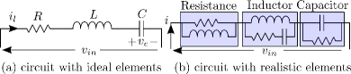
Figure 1: Schematic of R-L-C series circuit

There are some subtleties though. While the admittance of the circuit in Fig. 1(a) is passive, it is a strictly proper transfer function. Therefore, the impedance transfer function $Z(s)=\frac{(s^{2}LC+sRC+1)}{sC}$ is not proper, and therefore, it is not passive. Non-properness implies that $Z(s)\to\infty$ when $s\to\infty$, and that a connection to a current source will lead to a singularity. However, in practice, the distributed nature of the circuit elements always alleviates such issues. For example, the consideration of the parasitic elements (shown in Fig. 1(b)) ensures that both the impedance and the admittance of the circuit are bi-proper.

For a three-phase network, it is convenient to formulate the equations of the network in the D-Q frame. This is because most devices connected to the network are time-invariant in the D-Q domain, facilitating transfer function analyses. It is shown in [7] that the passivity of the impedance/admittance of any component in three-phase variables is retained under the synchronously rotating D-Q-o transformation. Therefore, the dynamical model of the T&D network is also passive with $(\Delta v_{D},\Delta v_{Q})$ and $(\Delta i_{D},\Delta i_{Q})$ as the input-output variables.

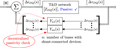
Figure 2: Scheme of passivity based stability criterion

Since the admittance/impedance of a T&D network is passive regardless of the the topology or the operating condition, this can be exploited to develop a local small-signal stability assessment scheme, as shown in Figure 2. In this scheme, the D-Q domain admittance (represented by $Y_{sj}(s)$ for device $j$ in Figure 2) of the shunt-connected devices need to be individually passive in order to ensure the stability of the system. However, the violation of the frequency domain passivity conditions by controlled power injection devices in the low frequency range restricts the applicability of this scheme [7]. To overcome this difficulty, the passivity of these components, when modelled using other input-output variables, is also examined. The choice of these alternative variables are motivated by the variables used in typical steady-state real and reactive power control strategies.

IV Model II variables: $(\Delta\phi,\Delta V_{n})$ and $(\Delta P,\Delta Q)$

The interface variables in this case are the active and reactive power injections and the polar components of the bus voltage. Let $P_{j}$ and $Q_{j}$ denote the active and reactive power injection at bus $j$ respectively, which are represented as follows.

$$P_{j}=v_{Dj}i_{Dj}+v_{Qj}i_{Qj}\,,\,Q_{j}=v_{Dj}i_{Qj}-v_{Qj}i_{Dj}$$ (2)

where $v_{Dj},v_{Qj},i_{Dj},i_{Qj}$ represent the instantaneous D-Q components of the bus voltage and current injection at bus $j$. The bus voltage angle $\phi_{j}$ and normalized magnitude $V_{nj}$ of bus $j$ are related to $v_{Dj}$ and $v_{Qj}$ as follows.

$$\phi_{j}=\tan^{-1}\left(\frac{v_{Dj}}{v_{Qj}}\right),\,V_{nj}=\sqrt{\frac{v_{Dj}^{2}+v_{Qj}^{2}}{v_{Djo}^{2}+v_{Qjo}^{2}}}$$

where the subscript $o$ denotes the quiescent value of the corresponding variable. The subscript $j$ is dropped from the respective notations to denote the vector variables. For example, $P$ and $Q$ represent the vector of active and reactive power injections at all buses respectively. If there are $n$ buses, then

$$\begin{aligned} v_{D}&=\text{diag}(v_{D1o},..,v_{Dno}),v_{Q}=\text{diag}(v_{Q1o},..,v_{Qno})\\ i_{D}&=\text{diag}(i_{D1o},..,i_{Dno}),i_{Q}=\text{diag}(i_{Q1o},..,i_{Qno})\end{aligned}$$ (3)

Note that diag($a,b$) represents a diagonal matrix with $a$ and $b$ as the diagonal entries. The equations of (2) are linearized, and their small-signal variations are represented as follows.

$$\begin{bmatrix}\Delta P(s)\\ \Delta Q(s)\end{bmatrix}=\begin{bmatrix}J_{11}(s)&J_{12}(s)\\ J_{21}(s)&J_{22}(s)\end{bmatrix}\begin{bmatrix}\Delta\phi(s)\\ \Delta V_{n}(s)\end{bmatrix}=J(s)\begin{bmatrix}\Delta\phi(s)\\ \Delta V_{n}(s)\end{bmatrix}$$

$J(s)$ is related to the D-Q admittance $Y_{DQ}(s)$ as follows.

$$J(s) =\left(\mathcal{E}Y_{DQ}(s)+\mathcal{C}\right)\mathcal{F}\quad\text{where }$$

$$\mathcal{E}=\begin{bmatrix}v_{D}&v_{Q}\\ -v_{Q}&v_{D}\end{bmatrix},\, \mathcal{C}=\begin{bmatrix}i_{D}&i_{Q}\\ i_{Q}&-i_{D}\end{bmatrix},\mathcal{F}=\begin{bmatrix}v_{Q}&v_{D}\\ -v_{D}&v_{Q}\end{bmatrix}$$ (4)

Note that $v_{D},v_{Q},i_{D}$ and $i_{Q}$ are defined in (3). The following property describes the passivity behaviour of the dynamical model of the T&D network when $(\Delta\phi,\Delta V_{n})$ and $(\Delta P,\Delta Q)$ are used as the interface variables.

IV-A Wide-band dynamical model

Property 1.

The dynamical model of a R-L-C network with $(\Delta P,\Delta Q)-(\Delta\phi,\Delta V_{n})$ as interface variables is not passive.

The proof is given in Appendix A-1. Although this restricts the applicability of passivity based scheme using wide-band models, a limited scheme of applicability for the slower transients using low frequency models is considered. The passivity of the low frequency model is now presented.

IV-B Low frequency model

For typical parameters, the natural modes of the T&D network model (in D-Q variables) usually lie in the high frequency range. Therefore, it is reasonable to represent the network by a static low-frequency model for slower transient studies. At low frequencies, the network transfer function can be approximated by $J_{LF}$, which is the unreduced form of the load-flow Jacobian matrix.

$$J_{LF}=J(0)=\begin{bmatrix}J_{LF11}&J_{LF12}\\ J_{LF21}&J_{LF22}\end{bmatrix}=\begin{bmatrix}J_{11}(0)&J_{12}(0)\\ J_{21}(0)&J_{22}(0)\end{bmatrix}$$ (5)

Note that $J_{LF}$ represents a static relation. Normally $J_{LF}$ is singular (with one zero eigenvalue), because there cannot be a unique solution for the phase angles for specified set of active and reactive power injections. $J_{LF}^{\mathcal{R}}=J_{LF}+J_{LF}^{T}$ may not be positive semi-definite because the shunt capacitances in the network often result in a negative eigenvalue. This implies that $J_{LF}$ may not be passive.

The non-passivity of $J_{LF}$ can be alleviated by requiring that some devices connected to the network “contribute” to the diagonal terms of $J_{LF22}$. This is in order to compensate the effect of the shunt capacitances. In practical terms, this means that at least some devices should contribute to voltage regulation through $\Delta Q-\Delta V_{n}$ droop control (“grid-forming” devices), as shown in Figure 3. The contribution, denoted by $k_{qv}^{c}$, has to be specified for each device by the T&D operator based on an evaluation of the eigenvalues of $J_{LF}^{R}$. The aim is to ensure that no eigenvalue of $J_{LF}^{R}$ is negative.

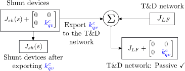
Figure 3: Contribution of devices to network passivity

Illustrative Example: The schematic of a network with controllable generators and loads is shown in Figure 4. The transmission line parameters and the equilibrium power flows are taken from the three-machine system of [8].

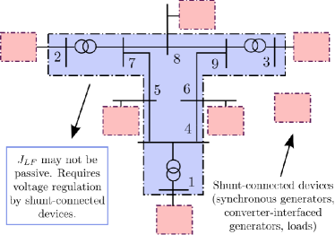
Figure 4: A network with controllable devices

The eigenvalues of $J_{LF}^{\mathcal{R}}$ are given in Table I. $J_{LF}$ is not passive as $J_{LF}^{\mathcal{R}}$ has a negative eigenvalue. If all the controllable generators and loads are able to contribute $\Delta Q=0.65\Delta V_{n}$ (in pu), then $J_{LF}$ becomes passive, as shown in the table.

Table I: Eigenvalues of $J_{LF}^{\mathcal{R}}$ of the three machine system

Base Case	Modified Case
$\mathbf{-0.84},0,7.52,8.50,10.15,$ $12.93,31.71,34.74,34.95,$ $36.29,41.37,42.8,93.51,94.52,$ $107.94,108.29,115.46,115.76$	$0,\mathbf{0.025},7.87,8.82,10.42,$ $13.13,32.43,35.06,35.44,36.53,$ $42.1,42.88,93.92,95.08,$ $108.29,109.06,115.72,116.61$
Reactive power-voltage regulation: 0.65 pu at buses 1, 2, 3, 5, 6, 8 each.

Lossless Model: The lossless approximation does not alleviate the non-passivity of $J_{LF}$. However, similar to the previous case, the non-passivity can be alleviated by contribution of voltage regulation by the shunt-connected devices.

This is also numerically verified using the three-machine system shown in Figure 4. The line resistances are neglected, and then $J_{LF}$ is calculated. The eigenvalues of $J_{LF}^{\mathcal{R}}$, with and without shunt voltage regulation contributions, are presented in Table II. Therefore, the low-frequency lossless T&D network model can also be passivated by borrowing voltage regulation capabilities from the shunt-connected devices.

Table II: Eigenvalues of $J_{LF}^{\mathcal{R}}$ of the three machine system

Base Case	Modified Case
$\mathbf{-0.84},0,7.8,8.83,10.32,$ $13.11,32.72,35.46,35.74,$ $36.79,41.72,43.16,94.37,95.34,$ $109,109.33,116.92,117.26$	$0,\mathbf{0.027},8.15,9.15,10.59,$ $13.31,33.44,35.86,36.11,37.07,$ $42.45,43.25,94.77,95.91,$ $109.33,110.1,117.2,118.09$
Reactive power-voltage regulation: 0.65 pu at buses 1, 2, 3, 5, 6, 8 each.

Decoupled Model $(J_{LF12}=J_{LF21}=0)$: For transmission network parameters, the off-diagonal blocks of $J_{LF}$ are usually much smaller than the diagonal blocks. Therefore, a further simplified model is also considered where $J_{LF12}=J_{LF21}=0$. This will be referred to as the “decoupled” model in this paper. The passivity behaviour is as follows.
(a) Decoupled lossy network: $J_{LF}$ is not passive.
(b) Decoupled lossless network: $J_{LF}$ is not passive if shunt capacitances are considered.
However, for both (a) and (b), voltage regulation by the shunt-connected devices can alleviate the non-passivity.
(c) $J_{LF}$ is passive in the case of decoupled lossless model, with shunt capacitances also neglected.

V Model III variables: $(\Delta P,\Delta Q)$ – $(\Delta\tilde{\omega},\Delta V_{n})$

In contrast to the input-output variables used in the previous case, the bus frequency deviation ($\tilde{\omega}$) is considered here instead of the bus phase angle. The derivative is approximated by using a small time-constant ($\tau$) as given in (6).

$$\Delta\tilde{\omega}(s)=\frac{s}{(1+s\tau)}\Delta\phi(s)$$ (6)

Let the transfer function of the T&D network in these variables be denoted by $J_{dp}(s)$. This is related to $J(s)$ as follows.

$$J_{dp}(s)=\begin{bmatrix}J_{11}(s)&J_{12}(s)\\ J_{21}(s)&J_{22}(s)\end{bmatrix}\begin{bmatrix}\frac{(1+s\tau)}{s}I&0\\ 0&I\end{bmatrix}$$ (7)

where $I$ is the identity matrix. The following property reflects the passivity behaviour of the dynamical model of the T&D network, when these input-output variables are considered.

V-A Wide-band dynamical model

Property 2.

The dynamical model of a R-L-C network with $(\Delta P,\Delta Q)-(\Delta\tilde{\omega},\Delta V_{n})$ as interface variables is not passive.

The proof is given in Appendix A-2. The passivity behaviour of the low frequency model is now presented.

V-B Low frequency model

The low frequency transfer function $N_{p}(s)$ is given in (8).

$$N_{p}(s)=J(0)\begin{bmatrix}\frac{(1+s\tau)}{s}I&0\\ 0&I\end{bmatrix}=\begin{bmatrix}\frac{J_{LF11}(1+s\tau)}{s}&J_{LF12}\\ \frac{J_{LF21}(1+s\tau)}{s}&J_{LF22}\end{bmatrix}$$ (8)

Note that $N_{p}(s)$ has a simple pole at $s=0$. For the system to be passive, the residue at $s=0$ must be positive semi-definite Hermitian. The expression of the residue of $N_{p}(s)$ evaluated at $s=0$, denoted by $S_{dp}\,$, is as follows.

$$S_{dp}=\lim_{s\to 0}sN_{p}(s)=\begin{bmatrix}J_{LF11}&0\\ J_{LF21}&0\end{bmatrix}$$ (9)

Note that $S_{dp}$ cannot be Hermitian if $J_{LF12}\neq 0$. Therefore, the low frequency model of the network in these variables cannot be passive, if coupled power flow models are considered.

Decoupled model: $S_{dp}$ in (9) is positive semi-definite if $J_{LF11}$ is Hermitian positive semi-definite. Note that $J_{LF11}$ is Hermitian only for lossless networks. Therefore, $N_{dp}(s)$ of decoupled lossy T&D network models is also not passive.

Lossless network: For decoupled lossless networks at $\Omega\neq 0$,

$$N^{\mathcal{R}}_{dp}(j\Omega)=N_{p}(j\Omega)+N_{p}^{T}(-j\Omega)=\begin{bmatrix}0&0\\ 0&J_{LF22}+J_{LF22}^{T}\end{bmatrix}$$

This may not be passive due to the presence of shunt capacitors. However, the non-passivity can be alleviated by contribution of voltage regulation by the shunt-connected devices. If the shunt capacitors are also neglected, then the network model is passive in these variables. This network model is used for passivity based stability analysis in [9].

Table III: Passivity of T&D network transfer function with different input-output variables

Model	Inputs	Outputs	Transfer function	Wide-band dynamic model	Low-frequency model
					Lossy (with $B$)	Lossless (with $B$)	Lossy (without $B$)	Lossless (without $B$)
Model I	$(\Delta i_{D},\Delta i_{Q})$	$(\Delta v_{D},\Delta v_{Q})$	$Z_{DQ}(s)$	✓	✓	✓	✓	✓
Model II	$(\Delta\phi,\Delta V_{n})$	$(\Delta P,\Delta Q)$	$J(s)$	✗	Coupled: ✗∗ Decoupled: ✗∗	Coupled: ✗∗ Decoupled: ✗∗	Coupled: ✗∗ Decoupled: ✗∗	Coupled: ✗∗ Decoupled: ✓
Model III	$(\Delta\tilde{\omega},\Delta V_{n})$	$(\Delta P,\Delta Q)$	$J_{dp}(s)$	✗	Coupled: ✗ Decoupled: ✗	Coupled: ✗ Decoupled: ✗∗	Coupled: ✗ Decoupled: ✗	Coupled: ✗ Decoupled: ✓
Model IV	$(\Delta\tilde{\omega},\Delta\tilde{V}_{n}^{d})$	$(\Delta P,\Delta Q)$	$J_{df}(s)$	✗	Coupled: ✗ Decoupled: ✗	Coupled: ✗∗ Decoupled: ✗∗	Coupled: ✗ Decoupled: ✗	Coupled: ✗∗ Decoupled: ✓
*: Non-passivity can be alleviated by borrowing voltage regulation capability of shunt-connected devices. $B$ denotes shunt capacitance.

VI Model IV variables: $(\Delta P,\Delta Q)$ – $(\Delta\tilde{\omega},\Delta\tilde{V}_{n}^{d})$

The input variables that are considered here are $\Delta\tilde{\omega}$ and the derivative of $\Delta V_{n}$, denoted by $\Delta\tilde{V}_{n}^{d}\,$. Similar to the evaluation of $\tilde{\omega}$ as given in (6), the derivative here is also approximated by the same time-constant $\tau$, as given in (10).

$$\Delta\tilde{V}_{n}^{d}(s)=\frac{s}{(1+s\tau)}\Delta V_{n}(s)$$ (10)

The transfer function in these variables $J_{df}(s)$ is related to $J(s)$ as follows.

$$J_{df}(s)=J(s)\times\frac{(1+s\tau)}{s}$$ (11)

The following property reflects the passivity behaviour of the dynamical model of the T&D network, when these input-output variables are considered.

VI-A Wide-band dynamical model

Property 3.

The dynamical model of a R-L-C network with $(\Delta P$, $\Delta Q)-(\Delta\tilde{\omega}$, $\Delta\tilde{V}_{n}^{d})$ as interface variables is not passive.

The proof is given in Appendix A-3. The passivity behaviour of the low frequency model is now presented.

VI-B Low frequency model

The low frequency model of the T&D network in these variables is represented by $N_{df}(s)$, which is given as follows.

$$N_{df}(s)=J_{LF}\times\frac{(1+s\tau)}{s}$$ (12)

$N_{df}(s)$ has a simple pole at $s=0$. For $N_{df}(s)$ to be passive, the residue, evaluated at $s=0$ has to be positive semi-definite Hermitian. The residue is $J_{LF}$, which is not Hermitian for lossy networks. Therefore, the low frequency model of lossy networks will not be passive in these input-output variables.

Lossless network: For lossless networks, $N_{df}$ is passive if and only if $J_{LF}$ is positive semi-definite. Although $J_{LF}$ may not be positive semi-definite with shunt capacitances considered, it can be achieved with voltage regulation contribution by the shunt-connected devices. If the shunt capacitances are neglected and decoupling is considered, then $J_{LF}$ is positive semi-definite Hermitian.

VII Conclusions and Future Work

The passivity behaviour of the T&D network transfer function for D-Q based rectangular and polar (and their derivatives) interface variables are summarized in Table III. The wide-band dynamic model of the impedance/admittance of the T&D network is passive. Although the wide-band models of the T&D network is not passive for the alternative interface variables considered here, the low-frequency models can be passivated by borrowing voltage regulation contributions from the shunt-connected devices. It is therefore necessary to ensure time-scale separation for decoupling the high and low frequency analysis in order to make the scheme viable. The decoupled analysis can use the rectangular variables for high frequency studies, and the polar variables for low frequency studies.

Appendix A Passivity of T&D network model

Let the state space matrices of the D-Q domain admittance $Y_{DQ}(s)$ be $(A_{y},B_{y},C_{y},D_{y})$. Then

$$D_{y}=\lim_{s\to\infty}Y_{DQ}(s)=\begin{bmatrix}D_{1}&\mathbf{0}\\ \mathbf{0}&D_{1}\end{bmatrix}$$ (13)

Note that $D_{1}$ is symmetric.

A-A Model II variables: $(\Delta P,\Delta Q)$ – $(\Delta\phi,\Delta V_{n})$

If the state-space matrices of the transfer function $J(s)$ are $(A_{2},B_{2},C_{2},D_{2})$, then $D_{2}=\left(\mathcal{E}D_{y}+\mathcal{C}\right)\mathcal{F}$, where $\mathcal{E},\mathcal{C}$ and $\mathcal{F}$ are defined in (4). It can be shown that the trace of $D_{2}+D_{2}^{T}$ is zero, indicating that it cannot be positive semi-definite. This violates the time domain conditions (see Section II-A). Therefore the system is not passive.

A-B Model III variables: $(\Delta P,\Delta Q)$ – $(\Delta\tilde{\omega},\Delta V_{n})$

If the state-space matrices of the transfer function $J_{dp}(s)$ are $(A_{3},B_{3},C_{3},D_{3})$, then

$$D_{3}=\left(\mathcal{E}D_{y}+\mathcal{C}\right)\mathcal{F}\begin{bmatrix}\tau I&0\\ 0&I\end{bmatrix}$$

where $I$ is the identity matrix. The diagonal entries of $D_{3}+D_{3}^{T}$ cannot be non-negative except when $i_{Do}v_{Qo}-i_{Qo}v_{Do}=0$, which indicates that the quiescent reactive power injection at each node is zero, which is quite unusual. If $i_{Do}v_{Qo}-i_{Qo}v_{Do}\neq 0$, then $D_{3}+D_{3}^{T}$ cannot be positive semi-definite. This will violate the time-domain passivity conditions (see Section II-A). Therefore, the system is not passive if $Q_{o}\neq 0$.

A-C Model IV variables: $(\Delta P,\Delta Q)$ – $(\Delta\tilde{\omega},\Delta\tilde{V}_{n}^{d})$

If the state-space matrices of the transfer function matrix $J_{df}(s)$ are $(A_{4},B_{4},C_{4},D_{4})$, then $D_{4}=\tau\left(\mathcal{E}D_{y}+\mathcal{C}\right)\mathcal{F}$, where $\mathcal{E},\mathcal{C}$ and $\mathcal{F}$ are as given in (4). Note that the trace of $D_{4}+D_{4}^{T}$ is zero, indicating that it cannot be positive semi-definite. This violates the time domain passivity conditions (see Section II-A). Therefore, it is not passive.

References

- [1] G. D. Irwin, A. K. Jindal, and A. L. Isaacs, “Sub-synchronous control interactions between type 3 wind turbines and series compensated AC transmission systems,” in 2011 IEEE Power and Energy Society General Meeting, 2011, pp. 1–6.
- [2] H. K. Khalil, Nonlinear Systems, 3rd ed. Prentice Hall, Upper Saddle River, New Jersey, 2002.
- [3] L. Harnefors, X. Wang, A. G. Yepes, and F. Blaabjerg, “Passivity-based stability assessment of grid-connected VSCs—An overview,” IEEE Journal of emerging and selected topics in Power Electronics, vol. 4, no. 1, pp. 116–125, 2015.
- [4] Y. Gu, W. Li, and X. He, “Passivity-Based Control of DC Microgrid for Self-Disciplined Stabilization,” IEEE Transactions on Power Systems, vol. 30, no. 5, pp. 2623–2632, 2015.
- [5] X. Wang, F. Blaabjerg, M. Liserre, Z. Chen, J. He, and Y. Li, “An active damper for stabilizing power electronics-based AC systems,” in 2013 Annual IEEE Applied Power Electronics Conference and Exposition, 2013, pp. 1131–1138.
- [6] L. Harnefors, M. Bongiorno, and S. Lundberg, “Input-admittance calculation and shaping for controlled voltage-source converters,” IEEE Transactions on Industrial Electronics, vol. 54, no. 6, pp. 3323–3334, 2007.
- [7] K. Dey and A. M. Kulkarni, “Analysis of the Passivity Characteristics of Synchronous Generators and Converter-Interfaced Systems for Grid Interaction Studies,” International Journal of Electrical Power & Energy Systems, vol. 129, pp. 1–12, 2021.
- [8] P. M. Anderson and A. A. Fouad, Power system control and stability, 2nd ed. John Wiley & Sons, Piscataway, NJ, 2003.
- [9] J. D. Watson and I. Lestas, “Control of Interlinking Converters in Hybrid AC/DC Grids: Network Stability and Scalability,” IEEE Transactions on Power Systems, vol. 36, no. 1, pp. 769–780, 2021.