A Multiwavelength Study of ELAN Environments (AMUSE2): Detection of a dusty star-forming galaxy within the enormous Lyman nebula at sheds light on its origin
1 Introduction
Studies of stellar mass functions in the nearby Universe have found that the stellar mass budget is dominated by the early type galaxies, in particular at the massive end ( M⊙; Bell et al. 2003; Kelvin et al. 2014; Moffett et al. 2016). These early type galaxies are found to predominantly locate in dense environments and have ceased to form new stars for at least the last several gigayears (Dressler, 1980; Thomas et al., 2010). These results suggest that the formation of the majority of the stellar masses of the massive galaxies happened at high redshifts, and within very active and dusty environments (Lilly et al., 1999). Indeed, one working hypothesis is that the progenitors of massive local ellipticals involve dusty star-forming galaxies (DSFGs) that are undergoing extensive star formation and black hole accretion via dynamically dissipative processes such as mergers (e.g., Narayanan et al. 2010; Chen et al. 2015), which subsequently transitioned to a quasar phase. The strong feedback from massive stars and black hole accretion quenches star formation and the growth of the black hole, turning the remains into compact quiescent galaxies. By merging these quiescent galaxies, eventually they become the local massive early-type galaxies (e.g., Hopkins et al. 2006; Alexander & Hickox 2012; Toft et al. 2014). While seemingly attractive, various places along this hypothetical formation and evolution path of the local massive ellipticals remain unclear. One such place is the transition between DSFGs and quasars. The intimate link between these two populations has been suggested from population studies. First, the evolution of black hole accretion rate density matches well in shape with that of star-formation rate density, both peaking at , during which the dominant star-forming population is the DSFG (Hopkins et al., 2007; Delvecchio et al., 2014; Madau & Dickinson, 2014). Second, from the point of view of large-scale spatial distribution, statistical measurements of auto-correlation functions of each population have inferred similar correlation lengths, i.e. comparable halo masses, within a wide redshift range of (Myers et al., 2006; Porciani & Norberg, 2006; Shen et al., 2007; Hickox et al., 2012; Eftekharzadeh et al., 2015; Chen et al., 2016a; Wilkinson et al., 2017; An et al., 2019; Lim et al., 2020; Stach et al., 2021). A certain level of overlap of the two populations in both space and time can find support from cross-correlation measurements (Wang et al., 2015), however, due to low space density of both populations, detailed assessments of their environmental connections, in particular on halo scales, have been difficult. One way to tackle this issue of low space densities is to conduct targeted far-infrared or submillimeter observations around selected samples of quasars, aiming to uncover and characterise physically associated DSFGs around central quasars. Indeed, via submillimeter number counts measured from single-dish surveys, populations of DSFGs have been statistically found on Mpc scales around various quasar samples such as high-redshift radio galaxies (HzRGs) and AGN selected from the Wide-field Infrared Survey Explorer(WISE) all-sky infrared survey (Stevens et al., 2003; Rigby et al., 2014; Dannerbauer et al., 2014; Zeballos et al., 2018), corroborating the co-existing nature on halo scales between DSFGs and quasars. On the other hand, interferometric observations have allowed discovery and characterisations of DSFGs around quasar samples on 100 kpc scales, often finding evidence of galaxy mergers that in principle helped trigger the vigorous activities in these regions (Ivison et al., 2012; Emonts et al., 2015; Gullberg et al., 2016; Trakhtenbrot et al., 2017; Decarli et al., 2018; Hill et al., 2019). However, these studies were often focused on individual cases or small samples, thus extending them into different kinds of quasars are needed to fully capture the environmental relations between DSFGs and quasars. To do so, we have initiated A Multiwavelength Study of ELAN Environments (AMUSE2) campaign, with the primary goal to study the multi-phase environment of quasars that host enormous Ly nebulae (ELANe; Arrigoni Battaia et al. 2018b, 2021; Nowotka et al. 2021), particularly from the far-infrared and submillimeter point of view. Only recently discovered, ELANe represent an extreme form of Ly emission at , which typically extend over kpc in physical scales with a surface brightness level of SB erg s-1 cm-2 arcsec-2 (Cantalupo et al., 2014; Hennawi et al., 2015; Cai et al., 2017, 2018, 2019; Arrigoni Battaia et al., 2018a). In order to explain the extreme Ly luminosity and the measured line ratios between Ly and CIV and HeII, detailed spectral synthesis modelling has suggested that these nebulae, powered by multiple sources, represent a large amount of dense ( cm-3) and cool ( K) gas with masses about 1010-11 M⊙ (Arrigoni Battaia et al., 2015; Hennawi et al., 2015; Cai et al., 2017). Molecular gas measurements based on CO(1-0) on one of the ELAN, the MAMMOTH-1 ELAN, have indeed shown a comparable amount of cold gas in the circumgalactic medium (CGM) around the powering quasars (Emonts et al., 2019). This large cool and cold gas reservoir could originate from cold accretion from the IGM or stripped/expelled gas from the infalling galaxies. Evidence also suggests the possibilities of undetected obscured sources to partly contribute to ELAN via softer ionizing radiations from star formation (Arrigoni Battaia et al., 2018a). In this paper we focus on a proto-typical ELAN, the Slug ELAN, which was first discovered by Cantalupo et al. (2014) using Keck narrow-band imaging. With an end-to-end size of about 450 kpc, the Slug ELAN remains one of the most luminous and the largest in Ly among all the Ly nebulae discovered so far (see Ouchi et al. (2020) for a review). Follow-up observations have painted a scenario where the nebula consists of multiple gaseous components that are distinct in kinematics. There appears to be three main kinematic structures; If referencing to UM287, the first is found to be at about km s-1, dubbed region c in Cantalupo et al. (2019), consisting of compact sources ‘C’ and ‘D’ reported by Leibler et al. (2018) as well as the He ii extended emission. The second component is at about km s-1, corresponding to the ’bright tail’ of the Ly nebula. And finally the third component of the Ly nebula can be found at about km s-1, which was dubbed region 1 by Leibler et al. (2018). Their origins are still in active discussion (Martin et al., 2015; Arrigoni Battaia et al., 2015; Leibler et al., 2018; Cantalupo et al., 2019). Here we complement the existing datasets from the submillimeter point of view, aiming to address whether there are DSFGs hidden from optical observations, and if yes what are the roles they play for the presence of the Slug ELAN. Throughout this paper we adopt the AB magnitude system (Oke & Gunn, 1983), and we assume the Planck cosmology: H 67.8 km s-1 Mpc-1, 0.31, and 0.69 (Planck Collaboration et al., 2014). At the redshift of the Slug ELAN, 2.28, the angular distance scale is 8.4 kpc for 1′′.2 Observations and data
2.1 ALMA
The 12-meter array observations were split into two execution blocks (EBs), both of which were carried out in mid-January 2019. During that period of time the baselines had a range from 15.1m to 313.7m, the mean precipitation water vapor was 3.6 mm, and at least 44 antenna were used to collect the data. The four science spectral windows were tuned to a band 4 standard FDM with 1920 channels, two of which were for continuum, and each of the remaining two was focused on redshifted CO(4-3) and [CI] 3P1 3P0 (hereafter [CI](1-0)), respectively. The primary beam full-width-half-maximum (FWHM) for band 4 with the 12-meter array is about 45′′ (380 kpc). The amplitude (flux) and bandpass calibrator was J0006-0623, and J0108+0135 was used for phase monitoring. The total on-source time given by the QA2 report is summed to 2.2 hours. We re-imaged the data to produce the optimal results. To do that, the raw visibilities were calibrated by running the corresponding scriptForPI.py scripts under casa version 5.4.0-68, meaning that we adopted the calibrations performed by the QA2 team members, who also noted that additional flagging was done on bad antennas DA55 and DA61 in phase calibrator. We confirm the quality of the reduction by examining the weblog. To make the imaging process more efficiently, the calibrated visibilities were first binned in channels by a factor of 10, resulting in a frequency resolution of 9.77 MHz, corresponding to a velocity resolution of 19-21 km/s depending on the exact frequency. We note that our detected lines are much broader than the binned channel width so this step does not affect any of the results. We then proceeded to continuum subtraction. The channels that contain significant line-emission were identified based on the delivered data cubes and excluded from continuum fitting. The identified continuum channels were used for both continuum generation and subtraction. While we later refer to all band-4 continuum as 2 mm continuum, the continuum for this data set has a nominal frequency at 145.1 GHz, so 2.07 mm in wavelength. We then used tclean to perform inverse Fourier transformation and clean on both the continuum and continuum-subtracted visibilities. The visibilities were transformed to images of 270270 pixels in x (RA) and y (DEC) axis with a pixel size of 03 (6-8 pixels per synthesized beam). Natural weighting for the baselines was chosen to enhance source detection, however later in the analyses we re-image the cubes with other weighting as needed. To increase the efficiency of clean, we adopted the auto-masking approach in Tclean, by setting the usemask papameter to ’auto-multithresh’, the noisethreshold parameter to 4, and the lownoisethreshold parameter to 2.5. The cubes within the masked regions determined by auto-masking were then cleaned down to 2 sigma level (nsigma = 2 in Tclean). Finally, given the same baseline weighting across the whole frequency range, the reduced cubes have different spatial resolution in each frequency channel. To allow more straightforward analyses and understanding of the data we applied smoothing on the reduced cubes by using the CASA routine Imsmooth, setting the kernel to the common resolution, which is normally the largest beam size of the pre-smoothed cube. After this step, the spatial resolution is the same across the image cubes, with a size of and a P.A. of degrees. The synthesized beam shape for the continuum is similar to that of the cubes, and a P.A. of also degrees. The final cleaned continuum image has a 1 sensitivity of 12.4 Jy/beam at 145 GHz, and the mean sensitivity for the cleaned image cube is about 300 Jy/beam per binned channel (9.77 MHz). The achieved sensitivities are consistent with the expected values from the sensitivity calculator.2.2 Multi-band imaging data
We exploit multiple waveband imaging data that we acquired in the past years for the Slug ELAN field: -band, -band, -band, 450 and 850 m. The -band (1 hour) and -band (10 hours) imaging data were taken with the Keck telescope using the LRIS instrument (Oke et al., 1995) on UT 12-13 November 2013. The reduction of the data was performed using standard techniques (see Cantalupo et al. 2014 for details). The -band imaging observations were carried out using the HAWK-I instrument (Casali et al. 2006) on the VLT on UT 17 October 2018 under clear weather (Program ID: 0102.C-0589(D), PI: F. Vogt). These data were acquired as 16 60s -band exposures to which it is applied a dithering within a jitter box of . The Slug ELAN was placed in the fourth quadrant of the HAWK-I field-of-view. We reduced these data as done in paper I, using the standard ESO pipeline version 2.4.3 for HAWK-I111https://www.eso.org/sci/software/pipelines/hawki/hawki-pipe-recipes.html. The flux calibration and astrometry are obtained using the 2MASS catalogue. The astrometry has an average error of . The seeing in the final combined image is . The submillimeter imaging at 450 and 850 m were taken with the SCUBA-2 camera (Holland et al., 2013) on the JCMT, and the procedures for reduction, calibration, as well as part of the 850 m results were presented in Nowotka et al. (2021) (Paper II). The Slug ELAN was located at the center of the daisy pattern used during observations. At this location the 450 and 850 m data have an rms of 11.7 and 1.02 mJy, respectively.3 Analyses and Results
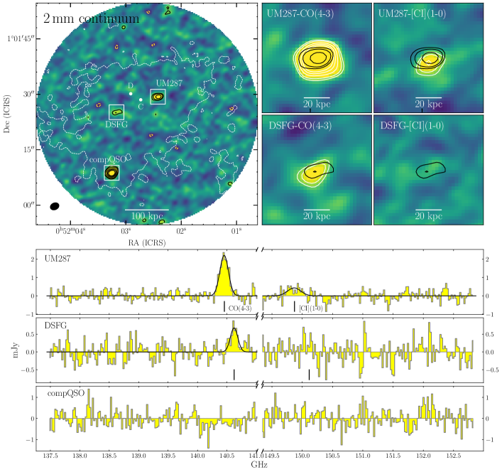 Figure 1: A gallery of our key ALMA results of both 2 mm continuum and emission lines toward the central regions of the Slug ELAN. Top-left: 2 mm continuum image, without primary beam correction, is linearly scaled from -4 to 5 , and roughly centered on the enormous Ly nebula.
The white dashed contours show the Ly surface brightness isophote of erg s-1 cm-2 arcsec-2 obtained from Keck narrow-band imaging (Cantalupo et al., 2014). The black solid contours show the positive 2 mm continuum signals at 3, 4, 6, 8, 10 , and the dashed yellow contours show the level of -3 . The three significant continuum detections, enclosed by the Ly isophote, are marked by white boxes with the corresponding abbreviated source names. The locations of compact sources ’C’ and ’D’ are shown for a clear overview of this system.
The synthesized beam shape and size are shown at the corner in black. Bottom: Spectra extracted at the three continuum detections respectively using apertures two times of the synthesized beam, with centroids determined through an iterative process detailed in Section 3.2. The line emission that are significantly detected are well fit by single-Gaussian models which are plotted as black curves, and the line identifications are indicated with short vertical segments. Note the spectra are broken in frequency to remove the gap due to the nature of the tuning. Top-right: Moment zero maps of the CO(4-3) and [CI](1-0) lines from UM287 and the DSFG, contoured by white curves with levels same as the continuum. For comparison the continuum is shown in black contours again with the same levels. The physical scale at the UM287 redshift is marked by scale bars as a reference.
Figure 1: A gallery of our key ALMA results of both 2 mm continuum and emission lines toward the central regions of the Slug ELAN. Top-left: 2 mm continuum image, without primary beam correction, is linearly scaled from -4 to 5 , and roughly centered on the enormous Ly nebula.
The white dashed contours show the Ly surface brightness isophote of erg s-1 cm-2 arcsec-2 obtained from Keck narrow-band imaging (Cantalupo et al., 2014). The black solid contours show the positive 2 mm continuum signals at 3, 4, 6, 8, 10 , and the dashed yellow contours show the level of -3 . The three significant continuum detections, enclosed by the Ly isophote, are marked by white boxes with the corresponding abbreviated source names. The locations of compact sources ’C’ and ’D’ are shown for a clear overview of this system.
The synthesized beam shape and size are shown at the corner in black. Bottom: Spectra extracted at the three continuum detections respectively using apertures two times of the synthesized beam, with centroids determined through an iterative process detailed in Section 3.2. The line emission that are significantly detected are well fit by single-Gaussian models which are plotted as black curves, and the line identifications are indicated with short vertical segments. Note the spectra are broken in frequency to remove the gap due to the nature of the tuning. Top-right: Moment zero maps of the CO(4-3) and [CI](1-0) lines from UM287 and the DSFG, contoured by white curves with levels same as the continuum. For comparison the continuum is shown in black contours again with the same levels. The physical scale at the UM287 redshift is marked by scale bars as a reference.
3.1 2 mm continuum
The cleaned 2 mm continuum of the central UM287 region is shown in Figure 1 along with its synthesized beam at the corner. To systematically identify significantly detected sources, we ran sextractor on both the original and inverted images and then determined a source-finding threshold above which there is no detection in the inverted image. We subsequently identified three sources that are above such a detection threshold, all of which have a peak signal-to-noise ratio of . These three sources, UM287, the dusty star-forming galaxy, and the companion quasar, are boxed in Figure 1 with their abbreviated names (UM287, Slug-DSFG, and compQSO). The sky coordinates deduced from sextractor were then used as the initial guess for the casa routine imfit, which was used to fit two-dimensional Gaussian profiles to measure the integrated flux densities and estimate their sizes. We found all three of them unresolved in the current image, as well as in images with higher spatial resolution (slightly under 2′′) produced with robust weighting in tclean. No meaningful size constraints can be derived. Since they are unresolved, we adopt the sky positions and the peak values from imfit for the three sources and the primary beam correction was applied to obtain the final flux density measurements. We have also used uvmultifit to conduct Gaussian fitting in the visibility space and the results are consistent with those derived from the image-base fitting. The measurements are provided in footnote 3 for the three continuum detected sources, and upper limits for source ’C’ and ’D’ are also provided for completeness. Table 1: Continuum and Line Measurements333Uncertainties in 1 are given in the parentheses and only the last decimal number is given if the measurements are precise to more than two decimal points. Upper limits are 6 based on the line finding code LineSeeker (Section 3.2). All flux densities have been corrected for the primary beam effects. In all cases CO represents CO(4-3) and [CI] stands for [CI](1-0) ID R.A. Decl. FWHM 444Line luminosities in units of 109K km/s pc. FWHM [J2000;deg] [J2000;deg] [mJy] [Jy km/s] [km/s] [Jy km/s] [km/s] UM287 13.010083 1.024816 0.11(0.01) 2.2825(1) 0.87(0.08) 368(25) 14(1) 2.2840(8) 0.24(0.10) 513(171) 3.4(1.5) Slug-DSFG 13.013202 1.023657 0.05(0.01) 2.2786(4) 0.23(0.07) 319(75) 3.7(1.2) N/A 0.23 N/A 3.3 compQSO 13.013560 1.019100 0.28(0.02) N/A 0.23 N/A 3.7 N/A 0.23 N/A 3.3 Source C 13.011378 1.024590 N/A 0.23 N/A 3.7 N/A 0.23 N/A 3.3 Source D 13.012132 1.025042 N/A 0.23 N/A 3.7 N/A 0.23 N/A 3.33.2 Line emission
To systematically search for line emission and quantify their significance, we ran the publicly available code LineSeeker, which was first written and used to search for line emission for the ALMA frontier field survey (González-López et al., 2017), and was later applied to the data taken for the ALMA Spectroscopic Survey in the Hubble Ultra Deep Field (ASPECS; Walter et al. 2016; González-López et al. 2019). Similar to another publicly available line searching code mf3d (Pavesi et al., 2018), LineSeeker utilizes a matched filtering kind of technique that combines spectral channels based on Gaussian kernels with a range of widths. The widths are chosen to match lines detected in real observations. LineSeeker was chosen for our data over mf3d since it was designed specifically for ALMA data cubes that have a similar spectral setting as that of our data. Comparisons between the two codes in fact show that both effectively return consistent results to within 10% (González-López et al., 2019). With LineSeeker we obtained three line detections at from two sources, with their sky locations matching those of the two continuum sources, UM287 and the Slug-DSFG. At this significance level there is no equivalent detection from the negative signal, which was at maximum at 5 level. The signal-to-noise of has also been shown to return robust detections by the ASPECS team. No significant line detection can be found from the companion quasar. As we show later this is likely due to the fact that the millimeter photometry is dominated by synchrotron radiation therefore most of the infrared luminosity is contributed by its super massive black hole, and the sensitivity of our ALMA observations is not sufficiently deep to detect the expected CO or [CI] lines given its relatively faint dust infrared luminosity. The final spectra were obtained in the following steps. Motivated by the results of LineSeeker and the fact that sources are not spatially resolved in continuum, we extract the spectra, first centered on the continuum positions, using elliptical apertures with a shape of the synthesized beam. The optimal aperture size to extract the total line flux density was determined by a curve-of-growth analysis, where Gaussian fits were performed on spectra extracted from beam apertures scaled by a range of factors from 0.25 to 2.5. The optimal aperture size was then determined to be the one that larger apertures do not return significantly higher flux densities, and we found for all the lines a factor of 2 of the synthesized beam is optimal. We then produced moment zero maps based on the spectra extracted from the optimal apertures and performed imfit to determine their sky positions. We then updated the aperture centroid to the coordinates deduced from imfit and iterated the above processes until all relevant measurements converge, including the sky locations, redshifts, and line properties. The results, after applying the primary beam correction, are provided in footnote 3 and the final spectra and their associated moment zero maps are plotted in Figure 1. Like the continuum, we found that the line emission are not spatially resolved, even if we push the spatial resolution to about 2′′ in major axis with the robust baseline weighting. In addition, the lines are all well described by a single-Gaussian profile, with reduced = 1.0. Lastly, considering the beam sizes and the significance of the detection, the sky locations of the emission lines are consistent with those of continuum, and we therefore only provide the continuum coordinates in footnote 3 to avoid confusion. Regarding the identification of the lines, we found the two lines detected at the direction of UM287 can only be CO(4-3) and [CI](1-0) assuming both were emitted from the same source.While the redshifts independently deduced from the two lines agree with each other to within 2 uncertainty, they both significantly deviate from 2.2790.001, the redshift typically adopted for UM287 based on its rest-frame optical spectra (McIntosh et al., 1999). Our measured redshift is also in agreement with that measured by Decarli et al. (2021) via CO(3-2), who reported 2.28240.0003. Unlike molecular line spectra, the optical spectra of quasars are complicated by blended Feii emission lines, and it often requires assuming certain Feii line templates in order to deduce redshifts. The uncertainty of this template assumption is difficult to quantify and normally not included in the quoted uncertainty. We therefore conclude that the most likely explanation of this offset in redshift is that the uncertainty of the optical redshift was underestimated. Assuming all redshifts agree, given that the one derived from CO(4-3) has the highest precision, we adopt the CO redshift for UM287 for this paper, i.e. . For the single line detection toward the Slug-DSFG, we estimate the probability of it being a random source on the sky and not associated with the UM287 system. We look at the probability from two angles; the line and the continuum. For the line, we estimate the probability by first assuming an empirically motivated redshift distribution model for the DSFG population in general and then integrating the corresponding redshift range from a list of line candidates with the observed frequencies lying within 2 from that of UM287. The redshift distribution of the general DSFG population is modelled as a lognormal function (equation 3 in Chen et al. 2016b) with a median of 1.85, of which the median is chosen to match the most recent result from Aravena et al. (2020), who focused on a sample of uniformly selected DSFG that has a similar continuum flux density as the Slug-DSFG. The list of line candidates considered includes CO with upper transition from J=2 to J=9 as well as the two lowest transition level [CI] lines. Lines with higher transition would infer a DSFG redshift of , which given our assumed redshift distribution model would have little impact in the estimates of the random probability. We include the two [CI] transition because given the recent survey of [CI] on DSFGs (e.g., Bothwell et al. 2017) we can not rule out their presence based on the line properties. In the end we find that the probability of detecting a non-associated line within the above set condition is about 1%. Now we turn to the continuum detection. The Slug-DSFG has a 2 mm continuum flux density of 50 Jy, roughly equivalent to 0.2 mJy at 1.2 mm assuming a dust emissivity index of 1.8. Based on the 1.2 mm number counts of the most recent ASPECS results (González-López et al., 2020) it is expected to find maximum 0.05 (considering upper 3 bound) sources given the effective area, the total area that is sensitive enough to detect a source with a flux density of the Slug-DSFG at . In combination, we conclude that the Slug-DSFG is associated with the UM287 system at a confidence level of ( from continuum multiplied by 1% from the line), and that detected line is CO(4-3), with a velocity difference of – km/s with respect to UM287 assuming that the redshift difference is solely due to peculiar velocity. Note that as seen in Figure 1 there is a 2 signal emitting from the frequency range of the expected [CI](1-0) line at the Slug-DSFG location. For the undetected lines we estimate the upper limits based on our S/N cut of 6 from LineSeeker. It just so happens that the CO line from the Slug-DSFG has a S/N of 6, we therefore adopt its integrated line flux density as the upper limit for all the undetected lines. This is likely a very conservative estimate since the S/N of 6 cut is based on a blind search without using the prior knowledge. For example by limiting the source redshift on specific lines the upper limits can be lowered. We however opt this approach for simplicity, and this choice does not affect our conclusions. In fact, adopting lower upper limits would strengthen some of the conclusions. The redshift of the companion quasar is assumed to be the same as that of UM287 (Cantalupo et al., 2014) and that for both source ’C’ and ’D’ is assumed to be 2.287 (Leibler et al., 2018). From now on the analyses are focused on the three sources that are detected in the ALMA data.3.3 Multi-band photometry and source properties
To estimate the physical properties of the three submilleter detected sources we perform model fitting on their spectral energy distributions (SEDs). We first obtain the photometry for all three sources. For , , and bands we ran SExtractor (Bertin & Arnouts, 1996) using our imaging data taken from the Keck telescope and the VLT. We adopt the MAG_AUTO photometric measurements provided by SExtractor, which are based on Kron-like elliptical apertures. For non-detections, we simply estimate the 3 upper limits by measuring the standard deviation of flux densities of 500 random, source-free positions using a 2′′ diameter aperture. The results are presented in Table 2. For the rest of the wavebands we cross match the three sources to the appropriate public catalogs and adopt the provided photometry measurements. We also estimate 3 upper limits wherever the imaging sensitivity is publicly available, which is the case for wavebands long-ward of Ks band except for the photometry adopted from the ALLWISE catalog, in which 5 upper limits are provided. Table 2: Multi-band photometry of the three main sources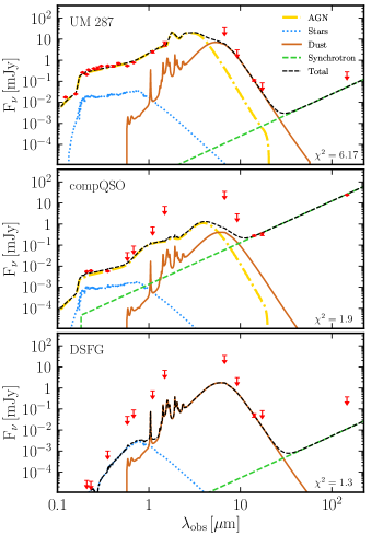 Figure 2: SED model fitting of all three sources. The wavebands considered are marked with red symbols, in which the
upper limits (Table 2) are shown as downward arrows and points with error bars for significant measurements. The curves are the best-fit models determined by cigale, color coded based on their constituent components, and the black dashed curves represent the sum of all components at a given wavelength. The reduced values of the best-fit models are given at the bottom-right corners.
Table 3: Physical properties obtained from the SED fitting
Figure 2: SED model fitting of all three sources. The wavebands considered are marked with red symbols, in which the
upper limits (Table 2) are shown as downward arrows and points with error bars for significant measurements. The curves are the best-fit models determined by cigale, color coded based on their constituent components, and the black dashed curves represent the sum of all components at a given wavelength. The reduced values of the best-fit models are given at the bottom-right corners.
Table 3: Physical properties obtained from the SED fitting4 Discussion
4.1 CO and [CI] line luminosity
To investigate the impact of dense environment on ISM-rich galaxies detected by our ALMA observations, we first discuss relations between line properties and infrared luminosity, and put them into the context with respect to other galaxy populations. To do so, we have compiled a list of other galaxy samples that have had reported measurements similar to those of our sources, meaning CO(4-3), [CI](1-0), line width in FWHM, and infrared luminosity. This list includes submillimeter galaxies (Bothwell et al., 2013; Alaghband-Zadeh et al., 2013; Bothwell et al., 2017; Birkin et al., 2021), quasars (Carilli & Walter, 2013; Bischetti et al., 2021), and one star-forming galaxy on the main sequence (Brisbin et al., 2019), star-forming galaxies on the main sequence (Valentino et al., 2018; Bourne et al., 2019; Boogaard et al., 2020), and local galaxy samples with Herschel FTS measurements (Kamenetzky et al., 2016). Since the compiled list consists of different studies focusing on various types of galaxies using at times different analysis methodologies to estimate source properties, such as infrared luminosity, it requires certain efforts to try homogenizing the measurements as much as possible. First, to avoid inconsistency due to different assumptions of cosmology, in all cases we deduce line luminosity based on the reported line flux densities, their associated uncertainties and the assumed cosmology in this paper. The line luminosity in K km s-1 pc2 is derived using the standard equation (Solomon & Vanden Bout, 2005), where is the total line flux in Jy km s-1, is the observed line frequency in GHz, and is the cosmological luminosity distance in Mpc. Secondly, we convert all the reported infrared luminosity to the one defined as the total luminosity at 8–1000 m, for which we assume = and = (Carilli & Walter, 2013). Comparisons of various measurements based on the stated calculations are now plotted in Figure 3. In the following we discuss them in detail. Note that the samples of galaxies include both lensed and unlensed sources, which are clearly separated in the plots. Since the lensing magnifications of all the reported lensed galaxies are assumed to be the same for both emission lines and infrared continuum, and as shown later the linear correlations have slopes consistent with unity, for clarity we plot the observed values without correcting for lensing. Figure 3: Top: Comparisons between line luminosity and infrared luminosity of the sources detected by the ALMA observations toward the Slug ELAN, as well as a compiled list of galaxy samples in the literature in both the nearby and high-redshift universe (See Section 4.1 for the included samples). The solid lines are best fit linear models to the star-forming galaxies, and the dashed one in the top-right panel shows the fit with the slope fixed but to the quasars only, which is a factor of 31 lower. Bottom-left: A diagram to effectively visualize the gas fraction in sample galaxies via a dynamical mass method (Section 4.2), indicating that on average quasars, including UM287 measured in this work, have a lower gas mass fraction compared to SMGs at similar redshifts. The Slug-DSFG appears to be at the lower end of the gas mass fraction, consistent with the top-left panel showing slightly under-luminous nature for the Slug-DSFG relative to the SMGs, which may be due to environmental effects. Bottom-right: A luminosity ratio diagram that helps visualize differences in physical parameters of the PDR in different galaxy populations. The model curves are based on the pdr toolbox described in Section 4.3. We find a denser field with stronger ultra-violet radiations in the PDR of quasars including UM287.
In the top panels of Figure 3 we plot comparisons between line luminosity and infrared luminosity, which provide insights into the conditions of interstellar medium and star formation in these galaxies. In both CO(4-3) and [CI](1-0), when considering all data points, we find a linear correlation in log-log scale with a best-fit slope of unity and a scatter of 0.3 dex. Upon closer inspections of each correlation, we find that for CO(4-3), both quasars and DSFGs lie on the general correlation. While for [CI](1-0), on the other hand, there is evidence of quasars being under luminous at fixed infrared luminosity. By fixing the slope we find the best-fit linear model for quasars is a factor of 31 lower in normalization than that of dusty star-forming galaxies, possibly suggesting either a more efficient star formation or a reduced amount of molecular gas in quasars, or both. Although as can be seen the total number of [CI](1-0) measurements on quasars is relatively small.
The different relationships between quasars and DSFGs seen in CO(4-3) and [CI](1-0) can be understood in their differences in excitation conditions of the ISM (e.g., Banerji et al. 2017; Fogasy et al. 2020). That is, if both quasars and DSFGs lie on the same - correlation to start with, the different luminosity ratios (0.46 and 0.87 for DSFGs555We assume the ratio for the SMGs is applicable to the main-sequence star-forming galaxies in our compiled list. and quasars respectively; Carilli & Walter 2013) would mean that the - linear relation for quasars would be a factor of about 2 lower than that for star-forming galaxies. If we instead adopt the latest conversion from SMGs for star-forming galaxies, which is 0.32 (Birkin et al., 2021), the difference would grow to a factor of about 3, even closer to our results since both CO(1-0) and [CI](1-0) line luminosity predominantly reflects molecular gas masses. Our results are consistent with recent report by Bischetti et al. (2021), who found CO(1-0) emission lines being systematically under luminous by a factor of compared to main-sequence galaxies and SMGs for a sample of WISE-SDSS selected hyper-luminous quasars.
One possible concern over the enhanced infrared luminosity at fixed line luminosity for quasars is the effectiveness of removing the AGN contribution. While the AGN contributions to the infrared luminosity have been carefully removed for our sources via the modelling of cigale, those for other quasars in the compiled list have not (Carilli & Walter, 2013; Bischetti et al., 2021), at least not specifically, although various methods were adopted to account for this effect. For example Carilli & Walter (2013) used a dusty star-forming galaxy SED template of Arp220 to estimate the infrared luminosity by fitting it to the submillimeter photometry, thus in principle the quoted infrared luminosity do not contain much AGN contributions. Furthermore, recent studies exploiting Herschel photometry on these lensed quasars have argued for star formation being the dominant contributor to the infrared luminosity, based on them having consistent infrared-to-radio correlation with that of star-forming galaxies (Stacey et al., 2018). In addition, studies with careful SED modelling to remove the AGN contributions on a sample of quasars have found similar results of under luminous CO (Perna et al., 2018). All these suggest that our results are not sensitive to the exact techniques used to remove the AGN contributions to the infrared luminosity.
For the sources detected in the Slug ELAN, both UM287 and the Slug-DSFG appear to lie close to the lower bound of the scatter based on the general correlations, which could suggest environmental effects on their cold gas reservoir. We look at this in more detail and continue this part of discussion in the next section.
Figure 3: Top: Comparisons between line luminosity and infrared luminosity of the sources detected by the ALMA observations toward the Slug ELAN, as well as a compiled list of galaxy samples in the literature in both the nearby and high-redshift universe (See Section 4.1 for the included samples). The solid lines are best fit linear models to the star-forming galaxies, and the dashed one in the top-right panel shows the fit with the slope fixed but to the quasars only, which is a factor of 31 lower. Bottom-left: A diagram to effectively visualize the gas fraction in sample galaxies via a dynamical mass method (Section 4.2), indicating that on average quasars, including UM287 measured in this work, have a lower gas mass fraction compared to SMGs at similar redshifts. The Slug-DSFG appears to be at the lower end of the gas mass fraction, consistent with the top-left panel showing slightly under-luminous nature for the Slug-DSFG relative to the SMGs, which may be due to environmental effects. Bottom-right: A luminosity ratio diagram that helps visualize differences in physical parameters of the PDR in different galaxy populations. The model curves are based on the pdr toolbox described in Section 4.3. We find a denser field with stronger ultra-violet radiations in the PDR of quasars including UM287.
In the top panels of Figure 3 we plot comparisons between line luminosity and infrared luminosity, which provide insights into the conditions of interstellar medium and star formation in these galaxies. In both CO(4-3) and [CI](1-0), when considering all data points, we find a linear correlation in log-log scale with a best-fit slope of unity and a scatter of 0.3 dex. Upon closer inspections of each correlation, we find that for CO(4-3), both quasars and DSFGs lie on the general correlation. While for [CI](1-0), on the other hand, there is evidence of quasars being under luminous at fixed infrared luminosity. By fixing the slope we find the best-fit linear model for quasars is a factor of 31 lower in normalization than that of dusty star-forming galaxies, possibly suggesting either a more efficient star formation or a reduced amount of molecular gas in quasars, or both. Although as can be seen the total number of [CI](1-0) measurements on quasars is relatively small.
The different relationships between quasars and DSFGs seen in CO(4-3) and [CI](1-0) can be understood in their differences in excitation conditions of the ISM (e.g., Banerji et al. 2017; Fogasy et al. 2020). That is, if both quasars and DSFGs lie on the same - correlation to start with, the different luminosity ratios (0.46 and 0.87 for DSFGs555We assume the ratio for the SMGs is applicable to the main-sequence star-forming galaxies in our compiled list. and quasars respectively; Carilli & Walter 2013) would mean that the - linear relation for quasars would be a factor of about 2 lower than that for star-forming galaxies. If we instead adopt the latest conversion from SMGs for star-forming galaxies, which is 0.32 (Birkin et al., 2021), the difference would grow to a factor of about 3, even closer to our results since both CO(1-0) and [CI](1-0) line luminosity predominantly reflects molecular gas masses. Our results are consistent with recent report by Bischetti et al. (2021), who found CO(1-0) emission lines being systematically under luminous by a factor of compared to main-sequence galaxies and SMGs for a sample of WISE-SDSS selected hyper-luminous quasars.
One possible concern over the enhanced infrared luminosity at fixed line luminosity for quasars is the effectiveness of removing the AGN contribution. While the AGN contributions to the infrared luminosity have been carefully removed for our sources via the modelling of cigale, those for other quasars in the compiled list have not (Carilli & Walter, 2013; Bischetti et al., 2021), at least not specifically, although various methods were adopted to account for this effect. For example Carilli & Walter (2013) used a dusty star-forming galaxy SED template of Arp220 to estimate the infrared luminosity by fitting it to the submillimeter photometry, thus in principle the quoted infrared luminosity do not contain much AGN contributions. Furthermore, recent studies exploiting Herschel photometry on these lensed quasars have argued for star formation being the dominant contributor to the infrared luminosity, based on them having consistent infrared-to-radio correlation with that of star-forming galaxies (Stacey et al., 2018). In addition, studies with careful SED modelling to remove the AGN contributions on a sample of quasars have found similar results of under luminous CO (Perna et al., 2018). All these suggest that our results are not sensitive to the exact techniques used to remove the AGN contributions to the infrared luminosity.
For the sources detected in the Slug ELAN, both UM287 and the Slug-DSFG appear to lie close to the lower bound of the scatter based on the general correlations, which could suggest environmental effects on their cold gas reservoir. We look at this in more detail and continue this part of discussion in the next section.
4.2 Molecular gas fraction and star formation efficiency
The results of under luminous CO and [CI] suggest higher efficiency of star formation, which could be due to relatively lower gas masses or relatively higher star-formation rates (SFRs) compared to the general SMG and main-sequence galaxies, or both. We investigate these possibilities by first looking at the gas mass fraction. We adopt both the dynamical and the direct methods; For the dynamical method we compare CO line widths and luminosity, which can be linked via a dynamical mass estimate expressed as , under the assumption of a rotation dominated system, where is the gravitational constant, is the circular velocity, is the representative radius, is the correction factor depending on the mass distributions and the adopted representative radius, and is the inclination angle. Assuming an exponential disk profile with a scale length and a half-light radius , it has been shown that and 666 for an exponential disk profile (Chen et al., 2015) are good approximations for spatially unresolved CO observations (de Blok & Walter, 2014). Under this assumption of an exponential disk is about 2 (Binney & Tremaine, 2008). In addition, dynamical masses can be linked to molecular gas masses with a gas mass fraction defined as where is stellar mass, and a dark matter fraction , such that . Assuming gas mass is dominated by molecular gas then gas masses are simply where is effectively a mass to light ratio to molecular hydrogen mass. With all these we can then re-write the equation of dynamical mass estimates to (1) , where FWHM is in km s-1 and in kpc, and we adopt (Tacconi et al., 2008). For dark matter fraction, we adopt based on the latest dynamical studies of star-forming galaxies with analyses of high-quality rotational curves (Genzel et al., 2020). In the bottom-left panel of Figure 3 we plot three lines representing three gas mass fractions respectively, in which we also plot our measurements along with those from the unlensed sources in the literature. For this exercise we also include the CO(3-2) measurements on a sample of quasars from Hill et al. (2019). To convert to we adopt the most up-to-date luminosity ratios reported in the literature, meaning / ratios of 0.87 and 0.32 for quasars and SMGs, respectively (Carilli & Walter, 2013; Birkin et al., 2021). For the CO(3-2) measurements on quasars reported in Hill et al. (2019) we adopt a again based on Carilli & Walter (2013). In addition, we adopt M⊙(K km s-1 pc2)-1 and kpc for SMGs and quasars (Chen et al., 2017; Tuan-Anh et al., 2017; Calistro Rivera et al., 2018; Badole et al., 2020; Bischetti et al., 2021). Note these adopted values are averages, and each of which comes with a range of uncertainties that are beyond the scope of this paper. The point of this exercise is to look for possible systematic differences between different galaxy populations thus the averaged values are sufficient. As we can see, in general the dusty star-forming galaxies have a higher gas fraction compared to that of quasars at similar redshifts. By fitting Equation 1 to the data we deduce a gas fraction of dusty star-forming galaxies of 0.50.1, compared to 0.20.1 for quasars, although each has about 0.3 dex scatter. For UM287 we find a gas fraction of 0.20.1, consistent with the average of the quasar sample, and 0.10.1 for the Slug-DSFG, on the lower end of the SMG sample. We now look at the direct method of computing gas mass fractions by taking the fractions between the molecular gas masses and stellar masses. By adopting the corresponding luminosity ratios, , and the given in footnote 3, we estimate molecular gas masses of and for UM287 and the Slug-DSFG, respectively, corresponding to gas fractions of and . We also estimate the weighted averaged gas fraction for the SMGs to be , in excellent agreement with that based on the dynamical method and the reported values for SMGs in the literature (Bothwell et al., 2013; Birkin et al., 2021). The large uncertainties for both UM287 and Slug-DSFG are due to the fact that the stellar masses are not well constrained, in particular for the Slug-DSFG. Despite that, their general behavior appears in agreement with the dynamical method, meaning that the gas fractions estimated from line emission tend to be lower for sources in the Slug ELAN, compared to other dusty star-forming galaxies at similar redshifts, suggesting that a lower gas mass could be the reason for them being under luminous as discussed in Section 4.1. On the other hand, given their SFRs and stellar masses UM287 and Slug-DSFG are located about 1-2 times the scatter above the main sequence so their SFRs are slightly enhanced. That is, the reasons of them being under luminous in line luminosity could be due to both smaller amount of gas reservoir and higher SFRs compared to star-forming galaxies at similar redshifts. Adopting the SFRs given in Table 3, which are averaged over 100 Myr based on the cigale SED models, the gas depletion timescales, defined as /SFR, are 418 Myr and 6443 Myr for UM287 and Slug-DSFG, respectively. The timescales would be 1910 Myr and 8495 Myr if we instead adopting the IR-base SFRs with the Kennicutt & Evans (2012) conversion. The typical depletion timescale for SMGs is about 200-300 Myr (Dudzevičiūtė et al., 2020; Birkin et al., 2021), which puts the Slug-DSFG at the lower end of the depletion time, again suggesting that it has relatively less gas which could be due to its extreme environments. It is worth noting that we can also estimate molecular gas masses using the measured [CI] luminosity. By following equation 6 of Bothwell et al. (2017) with a correction of helium contribution of 1.36 we find a [CI]-base molecular gas mass of M⊙ and M⊙ for UM287 and the Slug-DSFG, respectively; these are approximately a factor of two larger than the CO-base estimates. If the [CI]-base molecular gas masses are closer to the truth, then we will have to double the gas fraction and the depletion time, putting UM287 closer to the star-forming galaxies at similar redshifts under this context. However, like the known issue of the conversion factor, the [CI]-base estimates are also prone to the unknown nature of the [CI]/H2 abundance ratio, subject to variations of more than a factor of two. A standard ratio of was adopted for our calculation, which was estimated based on observations of M82 (Weiß et al., 2003). However, this ratio is known theoretically to vary by orders of magnitude under different local physical conditions such as density and radiation field (e.g., Papadopoulos et al. 2004), and observationally for high-redshift galaxies it lacks constraints that are free from other key assumptions such as and gas-to-dust ratio which are shown to heavily influence the results (Valentino et al., 2018). Given the circumstances it appears more appropriate to compare physical quantifies that are derived from similar measurements. Since most molecular gas masses reported in the literature and used for comparisons in this work are based on CO measurements, we opt to adopt the CO-base estimates. In summary, we tend to interpret that, like other quasars or AGN (Perna et al., 2018; Man et al., 2019; Bischetti et al., 2021), the gas fraction of UM287 is low and it is using up its gas reservoir very soon in less than 50 Myrs. On the other hand the Slug-DSFG appears to have less gas compared to typical SMGs at similar redshifts, perhaps due to the extreme environments around the ELAN that facilitate some level of gas stripping or strangulation. We extend this part of discussion in a later section.4.3 Physical parameters of the PDR
Line detection of multiple transitions and species in far-infrared and submillimeter allows simple modelling of physical conditions of the photo-dissociation region (PDR), in particular for high-redshift galaxies the luminosity-weighted mean hydrogen nucleus number density, , and the incident far-ultraviolet intensity, . In the bottom-right panel of Figure 3 we plot the luminosity ratios between / and /. We observe that UM287 is located at a similar locus as that of other quasars at similar redshifts, however it deviates notably from the main locus where most of the star-forming galaxies are located, such that the quasars have smaller values in both ratios. The upper limits of the Slug-DSFG put it in between the star-forming galaxies, and the main-sequence galaxies appear to offset from the SMGs toward higher / ratios. To model these ratios we adopt the pdr toolbox (Kaufman et al., 2006; Pound & Wolfire, 2008), which is a grid-base , minimizing model space fitting tool built upon various theoretical studies (Tielens & Hollenbach, 1985; Kaufman et al., 1999). The expected ratios given a range of constant and are plotted in Figure 3. We find that the majority of the star-forming galaxies have log()=4-4.5 cm-3 and log()=2.5-3.5 Habing, and the main-sequence galaxies have a similar range of but they are slightly lower in . The quasars including UM287 have on average about log()=4.5 cm-3 and log()=3.5 Habing, at the higher end of both and , suggesting denser and stronger far-ultraviolet radiation field. Our results on high-redshift star-forming galaxies are consistent with those reported recently by Valentino et al. (2020), who have studied similar line ratios on a sample of high-redshift galaxies in which they have also found a similar range of and in both star-forming galaxies and AGN or quasar samples. Our measurements on UM287 add to the existing measurements supporting that the PDR in quasars is denser and stronger in far-ultraviolet radiation field compared to star-forming galaxies at similar redshifts. We however caution that this exercise assumes that all line and dust emission originates from the PDR. The contributions from the X-ray dominated regions (XDR) on different transitions of CO lines for high-redshift quasars remain unclear. While some studies have found low- and mid- () CO to be predominantly emitted from the PDR (Pensabene et al., 2021), other studies have shown XDR could make significant contributions for CO transitions as low as (Uzgil et al., 2016; Bischetti et al., 2021). It is however unclear for CO(4-3). If a significant fraction of CO(4-3) is powered by the XDR, this would increase the [CI](1-0)-to-CO(4-3) ratios thus lower , moving it closer to the conditions of star-forming galaxies.4.4 Gas-to-dust ratios
With the estimates of molecular gas mass presented in Section 4.2 and the dust masses derived from cigale (Section 3.3), we can now look at the gas-to-dust ratios . As shown in Table 3, we find the two sources that have significant measurements in both quantities, UM287 and Slug-DSFG, have their about 20-30. This is significantly lower than the typical values of 100 estimated for other samples of quasars and dusty galaxies at similar redshifts (e.g., Shapley et al. 2020; Birkin et al. 2021; Bischetti et al. 2021), but consistent with what has been found for the quasars and AGN in another ELAN (Arrigoni Battaia et al., 2021). As a check we have also fit the 2 mm photometry with simpler modified black body (mBB) models. This is justified such that given the redshift of these sources the 2 mm photometry probes the Rayleigh-Jeans tail which is the part mainly determined by dust masses. Under the typical assumptions such that emission is isotropic over a spherical surface, optically thin, and single temperature, the model can be described as (2) where is the flux density at the observed frequency, is the rest frequency such that = (1+), is dust emissivity spectral index, and the rest-frame Planck function with a temperature . We can then deduce dust masses using (3) where is the luminosity distance at the source redshift and is the rest-frame dust mass absorption coefficient. In this case we adopt cm2g-1 at GHz (850 m) based on the dust model of Li & Draine (2001), for which a similar model was adopted in the cigale fitting. Assuming a range of dust emissivity spectral index of and dust temperature of that are appropriate for SMGs and quasars (Beelen et al., 2006; Carilli & Walter, 2013; Dudzevičiūtė et al., 2020), we find dust masses of 2-10 and 1-5 M⊙ for UM287 and Slug-DSFG, in good agreement with the estimates from cigale.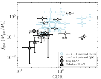 Figure 4: A plot contrasting gas-to-dust ratios (GDR) and gas fractions, where similar to Figure 3 the blue symbols represent the unlensed SMGs, the empty black for unlensed QSOs, and the filled black for sources in ELAN, including the two sources in the Slug ELAN (circles) and the three QSO and AGN in the Fabulous ELAN (triangles; Arrigoni Battaia et al. 2021).
With now two independent methods converging on dust mass estimates, it appears that the sources located within ELAN have both their gas fractions and gas-to-dust ratios on average lower than the typical SMGs found at similar redshifts. This intriguing finding motivated a detailed comparison between our sources in the Slug ELAN and other unlensed SMGs (Birkin et al., 2021) and unlensed quasars (Hill et al., 2019; Bischetti et al., 2021) at similar redshifts () reported in the literature. To increase the sample size of sources in ELAN, in this exercise we also include three quasars and AGN found in the Fabulous ELAN (Arrigoni Battaia et al., 2021), where CO(5-4) measurements were obtained and the dust masses were estimated using the same SED fitting parameters for cigale.
Since both gas fraction and gas-to-dust ratios may be affected significantly by a few underlying assumptions, it is important to homogenize the methodology if possible, or to understand the possible systematic differences if different methods were used. For gas-to-dust ratios, given the fact that the dynamical method can reproduce well the averaged fractions of the direct method (Section 4.2), we adopt the dynamical method for all the sources considered in this exercise, where the line widths and line intensities are provided. In practice, we fit the measurements of all the sources using Equation 1, under the same assumptions of parameters as those described in Section 4.2. This procedure ensures that the differences seen in gas fractions are not caused by the different assumptions of and sizes. Note that for the three sources that are found in the Fabulous ELAN, the spatially resolved CO(5-4) measurements in fact showed that they have half-light radius of 3-5 kpc, which are larger than our assumed 3 kpc for the dynamical method, and would further lower the gas fractions of these sources. Since we are interested in the averaged values we opt to adopt the same sizes.
On the other hand, for gas-to-dust ratios we adopt the reported CO line flux densities and compute gas masses based on the assumed cosmology of this paper and the adopted luminosity ratios presented in Section 4.2. For dust masses we simply adopt the reported values in the literature for the SMGs and quasars (Birkin et al., 2021; Hill et al., 2019; Bischetti et al., 2021). However, we caution that each study employed different methods for the infrared SED fitting and deducing dust masses, such as modified black body models or another SED fitting code magphys (da Cunha et al., 2008), adopting a range of dust emissivity spectral index () and dust mass absorption coefficient ( cm2g-1 at 850 m). While a detailed comparison of different dust modeling on these sources is outside the scope of this paper, previous studies using other galaxy samples have shown these different models to impact the results on a level of about a factor of two (e.g., Magdis et al. 2012).
Figure 4: A plot contrasting gas-to-dust ratios (GDR) and gas fractions, where similar to Figure 3 the blue symbols represent the unlensed SMGs, the empty black for unlensed QSOs, and the filled black for sources in ELAN, including the two sources in the Slug ELAN (circles) and the three QSO and AGN in the Fabulous ELAN (triangles; Arrigoni Battaia et al. 2021).
With now two independent methods converging on dust mass estimates, it appears that the sources located within ELAN have both their gas fractions and gas-to-dust ratios on average lower than the typical SMGs found at similar redshifts. This intriguing finding motivated a detailed comparison between our sources in the Slug ELAN and other unlensed SMGs (Birkin et al., 2021) and unlensed quasars (Hill et al., 2019; Bischetti et al., 2021) at similar redshifts () reported in the literature. To increase the sample size of sources in ELAN, in this exercise we also include three quasars and AGN found in the Fabulous ELAN (Arrigoni Battaia et al., 2021), where CO(5-4) measurements were obtained and the dust masses were estimated using the same SED fitting parameters for cigale.
Since both gas fraction and gas-to-dust ratios may be affected significantly by a few underlying assumptions, it is important to homogenize the methodology if possible, or to understand the possible systematic differences if different methods were used. For gas-to-dust ratios, given the fact that the dynamical method can reproduce well the averaged fractions of the direct method (Section 4.2), we adopt the dynamical method for all the sources considered in this exercise, where the line widths and line intensities are provided. In practice, we fit the measurements of all the sources using Equation 1, under the same assumptions of parameters as those described in Section 4.2. This procedure ensures that the differences seen in gas fractions are not caused by the different assumptions of and sizes. Note that for the three sources that are found in the Fabulous ELAN, the spatially resolved CO(5-4) measurements in fact showed that they have half-light radius of 3-5 kpc, which are larger than our assumed 3 kpc for the dynamical method, and would further lower the gas fractions of these sources. Since we are interested in the averaged values we opt to adopt the same sizes.
On the other hand, for gas-to-dust ratios we adopt the reported CO line flux densities and compute gas masses based on the assumed cosmology of this paper and the adopted luminosity ratios presented in Section 4.2. For dust masses we simply adopt the reported values in the literature for the SMGs and quasars (Birkin et al., 2021; Hill et al., 2019; Bischetti et al., 2021). However, we caution that each study employed different methods for the infrared SED fitting and deducing dust masses, such as modified black body models or another SED fitting code magphys (da Cunha et al., 2008), adopting a range of dust emissivity spectral index () and dust mass absorption coefficient ( cm2g-1 at 850 m). While a detailed comparison of different dust modeling on these sources is outside the scope of this paper, previous studies using other galaxy samples have shown these different models to impact the results on a level of about a factor of two (e.g., Magdis et al. 2012).
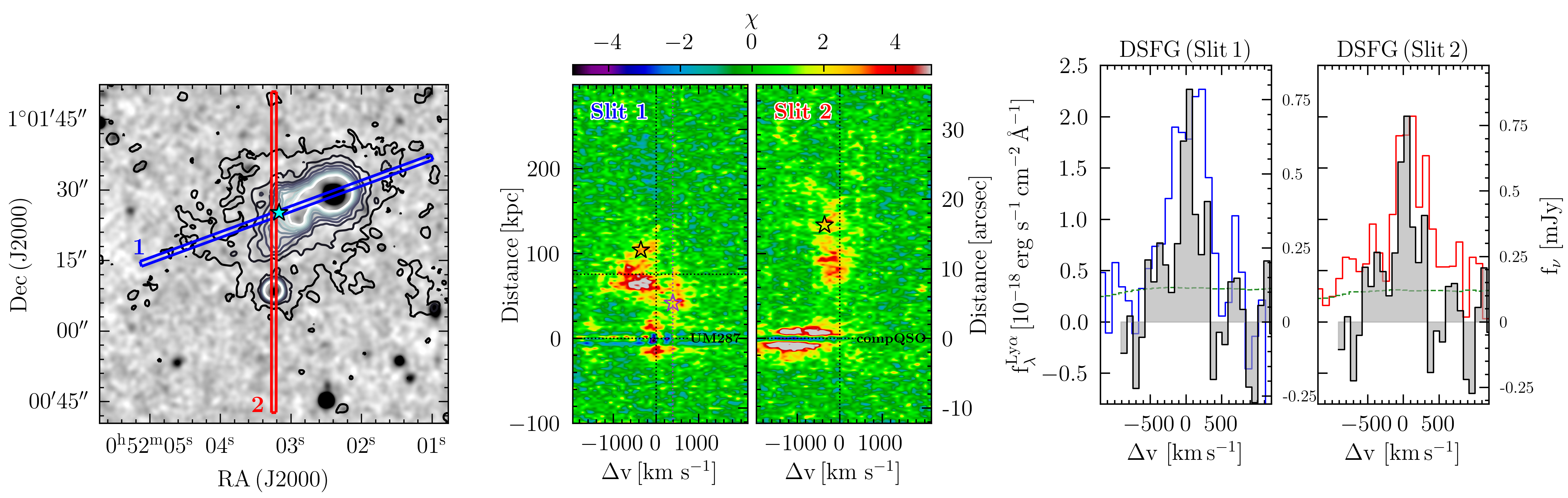 Figure 5: The spatial and spectral location of the DSFG in comparison to the Slug ELAN. Left: HAWK-I/-band map with overimposed the two Keck/LRIS slits of (slit 1 in blue and slit 2 in red; Arrigoni Battaia et al. 2015) and the contours for the Ly emission in the range S/N in steps of 5 (Cantalupo et al. 2014). The discovered DSFG (star) is inside slit 1 and right next slit 2. Middle: Keck/LRIS 2D spectra at the location of the Ly line (Arrigoni Battaia et al. 2015). The reference velocity is the systemic redshift of the quasar UM287 ().The DSFG is indicated by the black star. For reference, the position of source “c” (purple star) and the average He II velocity (vertical purple dashed line) are indicated (Cantalupo et al. 2019).
Right: Comparison of the 1D spectrum in Ly (extracted within a aperture) and CO(4-3) for the DSFG. The reference velocity is the systemic redshift of the DSFG (). The two Ly lines are plotted at the same flux density scale indicated on the left y-axis, while the CO(4-3) lines for comparison are normalized to the peak of each Ly line and their flux density scales are shown on each of their right y-axis.
We plot the results in Figure 4, where the sources in ELAN appear offset toward lower ends in both gas fraction and gas-to-dust ratio. Quantitatively, the medians with bootstrapped errors for gas fraction are , , and , for SMGs, quasars, and sources in ELAN respectively, and , , and for gas-to-dust ratios, respectively. That is, given the uncertainties the differences appear significant ( ) between SMGs and the sources in ELAN on both gas fractions and gas-to-dust ratios, while the difference in gas fraction between SMGs and quasars appear marginal (2 ).
As suggested by the analyses in Section 4.2, the general trend of quasars and AGN having lower gas fractions than SMGs is consistent with the evolutionary scenario where the quasar phase follows the SMG phase such that the quasars are closer in using up their cold ISM reservoir (Toft et al., 2014), which has also been suggested by other studies of molecular gas content in quasars (Perna et al., 2018; Hill et al., 2019; Bischetti et al., 2021).
On the other hand, while possible systematic differences in the reported dust masses need to be understood further, the apparently lower gas-to-dust ratios between sources in ELAN and the comparison samples of SMGs and quasars is intriguing. Given the observed correlation between gas-to-dust ratios and gas-phase metallicities in both nearby and high-redshifts galaxies (De Vis et al., 2019; Shapley et al., 2020), it may be that the sources in ELAN are more metal rich. However the measured ratios would imply a metallicity that is about two times the solar metallicity based on correlations provided by Leroy et al. (2011) and De Vis et al. (2019).
Physically this may be a result of gas stripping caused by active dynamical interactions in dense environments, leading to a higher gas-phase metallicity which is essentially a oxygen-to-hydrogen abundance ratio. This scenario may find support from the recent findings of more compact sizes of dust continuum compared to gas and stellar emission in dusty galaxies (e.g., Chen et al. 2017; Calistro Rivera et al. 2018; Tadaki et al. 2019), where stronger stripping effects on gas than dust may be expected, which would lower the gas-to-dust ratios. On the other hand, it could also be due to strangulation where the gas supply is made inefficient by the hot halos, such that metallicity increases as a function of time with continuous star formation as well as decreasing the gas-to-dust ratios (Hirashita, 1999; Peng et al., 2015). Finally, it is known that the circumgalactic medium of quasars is already metal enriched (about one third of solar; Lau et al. 2016; Fossati et al. 2021), thus depending on the timescales it is also possible that the accretion of enriched gas onto galaxies helps elevate the gas-phase metalicity. We further extend this discussion in the later sections.
Figure 5: The spatial and spectral location of the DSFG in comparison to the Slug ELAN. Left: HAWK-I/-band map with overimposed the two Keck/LRIS slits of (slit 1 in blue and slit 2 in red; Arrigoni Battaia et al. 2015) and the contours for the Ly emission in the range S/N in steps of 5 (Cantalupo et al. 2014). The discovered DSFG (star) is inside slit 1 and right next slit 2. Middle: Keck/LRIS 2D spectra at the location of the Ly line (Arrigoni Battaia et al. 2015). The reference velocity is the systemic redshift of the quasar UM287 ().The DSFG is indicated by the black star. For reference, the position of source “c” (purple star) and the average He II velocity (vertical purple dashed line) are indicated (Cantalupo et al. 2019).
Right: Comparison of the 1D spectrum in Ly (extracted within a aperture) and CO(4-3) for the DSFG. The reference velocity is the systemic redshift of the DSFG (). The two Ly lines are plotted at the same flux density scale indicated on the left y-axis, while the CO(4-3) lines for comparison are normalized to the peak of each Ly line and their flux density scales are shown on each of their right y-axis.
We plot the results in Figure 4, where the sources in ELAN appear offset toward lower ends in both gas fraction and gas-to-dust ratio. Quantitatively, the medians with bootstrapped errors for gas fraction are , , and , for SMGs, quasars, and sources in ELAN respectively, and , , and for gas-to-dust ratios, respectively. That is, given the uncertainties the differences appear significant ( ) between SMGs and the sources in ELAN on both gas fractions and gas-to-dust ratios, while the difference in gas fraction between SMGs and quasars appear marginal (2 ).
As suggested by the analyses in Section 4.2, the general trend of quasars and AGN having lower gas fractions than SMGs is consistent with the evolutionary scenario where the quasar phase follows the SMG phase such that the quasars are closer in using up their cold ISM reservoir (Toft et al., 2014), which has also been suggested by other studies of molecular gas content in quasars (Perna et al., 2018; Hill et al., 2019; Bischetti et al., 2021).
On the other hand, while possible systematic differences in the reported dust masses need to be understood further, the apparently lower gas-to-dust ratios between sources in ELAN and the comparison samples of SMGs and quasars is intriguing. Given the observed correlation between gas-to-dust ratios and gas-phase metallicities in both nearby and high-redshifts galaxies (De Vis et al., 2019; Shapley et al., 2020), it may be that the sources in ELAN are more metal rich. However the measured ratios would imply a metallicity that is about two times the solar metallicity based on correlations provided by Leroy et al. (2011) and De Vis et al. (2019).
Physically this may be a result of gas stripping caused by active dynamical interactions in dense environments, leading to a higher gas-phase metallicity which is essentially a oxygen-to-hydrogen abundance ratio. This scenario may find support from the recent findings of more compact sizes of dust continuum compared to gas and stellar emission in dusty galaxies (e.g., Chen et al. 2017; Calistro Rivera et al. 2018; Tadaki et al. 2019), where stronger stripping effects on gas than dust may be expected, which would lower the gas-to-dust ratios. On the other hand, it could also be due to strangulation where the gas supply is made inefficient by the hot halos, such that metallicity increases as a function of time with continuous star formation as well as decreasing the gas-to-dust ratios (Hirashita, 1999; Peng et al., 2015). Finally, it is known that the circumgalactic medium of quasars is already metal enriched (about one third of solar; Lau et al. 2016; Fossati et al. 2021), thus depending on the timescales it is also possible that the accretion of enriched gas onto galaxies helps elevate the gas-phase metalicity. We further extend this discussion in the later sections.
4.5 Ly-emitting gas from the Slug-DSFG
To understand the origin of the Ly nebula, in Arrigoni Battaia et al. 2015) we measured and modeled the properties of Ly, He ii, and C iv lines using two slits of deep LRIS spectra taken from the Keck telescope. Their respective locations and orientations are shown in Figure 5. Coincidentally, the newly discovered Slug-DSFG, marked as stars in the figure, is located almost right at the intersection of the two slits. While one of the slits (slit 2) covers only part of the source, the other one (slit 1) goes through the source entirely. What is even more remarkable is that Ly is clearly emitting from the locations of the Slug-DSFG, in both real and velocity spaces. We first extract spectra using the same circular aperture with a size of 2′′ in diameter as that used for extracting optical photometry (Section 3.3). In the right panel of Figure 5 we show the line profiles of Ly from the two slits, and compare them to the CO(4-3) line normalized to the peaks of Ly. We fit the line profiles with single Gaussian models and find Ly line luminosities of and erg s-1 with widths in FWHM of 63270 and 1200120 km s-1 from slit 1 and 2, respectively. Since slit 2 covers Slug-DSFG only partially, in principle the line luminosity should be smaller than that measured from slit 1, and the line widths should agree with each other. The fact that we are getting more emission and a wider line width from slit 2 could mean that the aperture size is too large such that it also covers emission coming from the gas surrounding the Slug-DSFG. This could be due to additional gas motions such as inflow or outflow, and as discussed in the later sections we attribute it mainly to gas ram pressure stripping. Indeed, if we extract the spectra using a 1′′ circular aperture instead, the line width appears consistent with that obtained from slit 1, and the line luminosity from slit 2 is indeed smaller than that from slit 1. We therefore adopt the Ly line luminosity and width from slit 1, which are erg s-1 and 63270 km s-1, and conclude that the broader component from slit 2 is due to the surrounding gas that is presumably undergoing gas mixing as part of the stripping process. The good agreement on the systemic velocity between Ly and the line detected by our ALMA data strengthens the argument that the line is CO(4-3).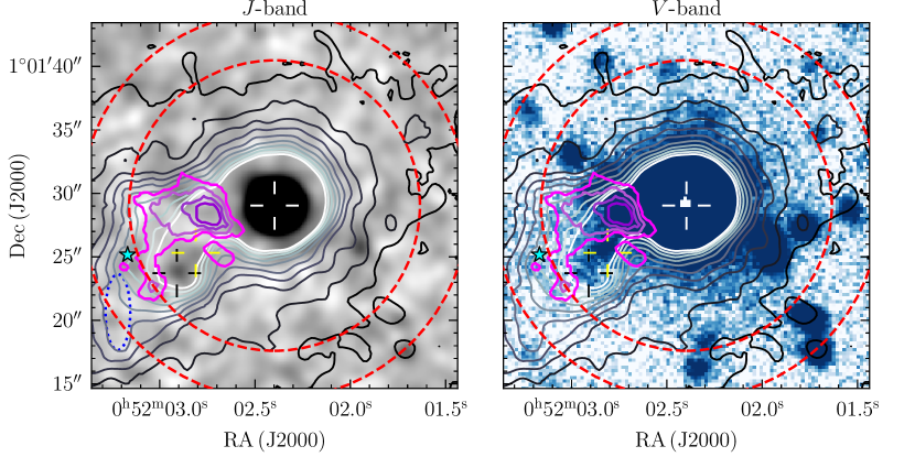 Figure 6: Left: HAWKI -band data with overimposed the Ly contours as in Figure 5 and the 2, 4, 6, 8 S/N contours for the He II emission associated with source “C” (magenta to purple; Cantalupo et al. 2019). The DSFG is indicated by the cyan star, while UM287 and the two continuum sources co-locating with the bright tail (detail given in Section 4.6.2) are indicated with white, black, and yellow crosshairs, respectively. The dotted blue ellipse indicates the area used in the calculation of the stripped material (section 4.6.3). Right: Same as the left panel, but for the LRIS -band. Continuum emission is evident within the brightest portion of the ELAN.
We investigate the origin of Ly by looking at the possibility of it originated from the Slug-DSFG itself due to recombination. Given the estimated SFRs we expect the intrinsic Ly luminosity of Slug-DSFG to be erg s-1, assuming a case B recombination ratio in luminosity of /=8.7 (Henry et al., 2015) and the conversion between H and SFR provided in Kennicutt & Evans (2012). Dust attenuation is estimated to be based on the best-fit SED model, however a Bayesian analysis performed by cigale shows , suggesting a highly skewed probability distribution. If is adopted, and assuming a Calzetti attenuation curve, the expected observed Ly luminosity should have been about erg s-1. If the probabilistic distribution is adopted for the expected Ly luminosity is instead erg s-1. These values appear in agreement with each other due to large uncertainties. It therefore remains inconclusive regarding the origin of the Ly emission from the Slug-DSFG, in particular whether it mostly emits from the Slug-DSFG via recombination, or due to scattering of other nearby sources from co-moving gas around the Slug-DSFG.
Figure 6: Left: HAWKI -band data with overimposed the Ly contours as in Figure 5 and the 2, 4, 6, 8 S/N contours for the He II emission associated with source “C” (magenta to purple; Cantalupo et al. 2019). The DSFG is indicated by the cyan star, while UM287 and the two continuum sources co-locating with the bright tail (detail given in Section 4.6.2) are indicated with white, black, and yellow crosshairs, respectively. The dotted blue ellipse indicates the area used in the calculation of the stripped material (section 4.6.3). Right: Same as the left panel, but for the LRIS -band. Continuum emission is evident within the brightest portion of the ELAN.
We investigate the origin of Ly by looking at the possibility of it originated from the Slug-DSFG itself due to recombination. Given the estimated SFRs we expect the intrinsic Ly luminosity of Slug-DSFG to be erg s-1, assuming a case B recombination ratio in luminosity of /=8.7 (Henry et al., 2015) and the conversion between H and SFR provided in Kennicutt & Evans (2012). Dust attenuation is estimated to be based on the best-fit SED model, however a Bayesian analysis performed by cigale shows , suggesting a highly skewed probability distribution. If is adopted, and assuming a Calzetti attenuation curve, the expected observed Ly luminosity should have been about erg s-1. If the probabilistic distribution is adopted for the expected Ly luminosity is instead erg s-1. These values appear in agreement with each other due to large uncertainties. It therefore remains inconclusive regarding the origin of the Ly emission from the Slug-DSFG, in particular whether it mostly emits from the Slug-DSFG via recombination, or due to scattering of other nearby sources from co-moving gas around the Slug-DSFG.
4.6 The origin of the Slug ELAN
4.6.1 Brief overview
Since the discovery of the Slug ELAN via narrow-band imaging (Cantalupo et al., 2014), various follow-up observations have been made to study the origin of this exceptional Ly structure which was initially interpreted as an intergalactic filament. Martin et al. (2015) imaged the nebula with the Palomar Cosmic Web Imager (PCWI), which allows studies of kinematic properties of Ly emission via integral field observations, and they found that the brightest Ly emission region appears to be an extended rotating hydrogen disk with a diameter of about 125 kpc in physical distance, possibly suggesting a cold flow disk similar to those predicted by some models (Stewart et al., 2011). In the meantime, deep long-slit spectra taken from the Keck telescope were taken on various slit positions and angles, targeting multiple lines such as H, N ii, He ii, and C iv, on both the nebula and a few selected nearby compact sources (Arrigoni Battaia et al., 2015; Leibler et al., 2018). Through the measured line ratios between Ly and H, as well as those between Ly and He ii, it has been suggested that the nebula is highly ionized, and has high gas densities ( cm-3) and large clumping factors (). In addition, with these higher velocity resolution observations they were able to resolve the kinematic structures into a few distinct components, suggesting a more complex dynamical nature of the nebula than that suggested by the results from Martin et al. (2015). The hypothesis of having distinct kinematic components has recently found support from deep MUSE observations where sharp variations of Ly-to-He ii line ratios have been reported (Cantalupo et al., 2019). Understanding each of these kinematic components would help capture the full picture regarding the origin of the Slug ELAN. As reviewed in the Section 1 and now more clearly shown in the middle panel of Figure 5, there appears to be three main kinematic structures; If referencing to UM287, the first is found to be at about km s-1, dubbed region c in Cantalupo et al. (2019), consisting of source ’C’ and ’D’ as well as the He ii extended emission. The second component is at about km s-1, corresponding to the ’bright tail’ of the Ly nebula. And finally the third one can be found at about km s-1, which was dubbed region 1 by Leibler et al. (2018).4.6.2 Revisiting the bright tail
In addition to the Slug-DSFG, our new -band image has yielded a new continuum detection (RA (J2000): 00:52:02.90 Dec(J2000):+01:01:23.85) that may be part of the ’bright tail’. As shown in Figure 6, the newly detected -band continuum is marked by black crosses, and it is located at exactly the end of the bright tail where there are also -band continuum emissions. The measured -band flux density is 22.050.05 (signal-to-noise ratio of 20) in AB magnitude. Given the number density of our -band image, the probability of finding a source brighter than this flux density by chance within a 1′′ radius circular area centered at the detected location, roughly the size of the end of the bright tail, is about 1%. While we do not have redshift measurements to confirm its association to the ELAN, the low probability of a random chance projection means that this -band source could be part of the bright tail. Previously, the bright tail has been proposed to be a gas component that sits much further away from UM287 compared to regions ’c’ (Cantalupo et al., 2019). This is based on the fact that the measured Ly luminosity is much fainter than expected if instead it is the much higher gas density, not further distances, that drives the low He ii-to-Ly ratio. However, together with the -band continuum the newly discovered -band continuum source could complicate the scenario. First the existence of a mJ=22 continuum source suggests that it is likely a galaxy, like the -band continuum source (RA (J2000): 00:52:02.81 Dec(J2000):+01:01:25.79), with a ISM type of density so much higher than the one typically assumed for halo gas, which may additionally serve to obscure Ly and He ii. Indeed, the fact that the southern edges of He ii emission appearing to go around the two continuum sources could suggest that they are attenuated by these two sources that are possibly sitting in between the line-of-sight to region ’c’. With the possibility of galaxies being present in the bright tail and causing obscuration, one may need to re-evaluate all the possible factors, including distances, gas densities, and scattering effects, considering the observed Ly luminosity and HeII-to-Ly ratios, in order to understand its origin. Without knowing the exact redshifts of these two continuum sources we defer this exercise to future studies.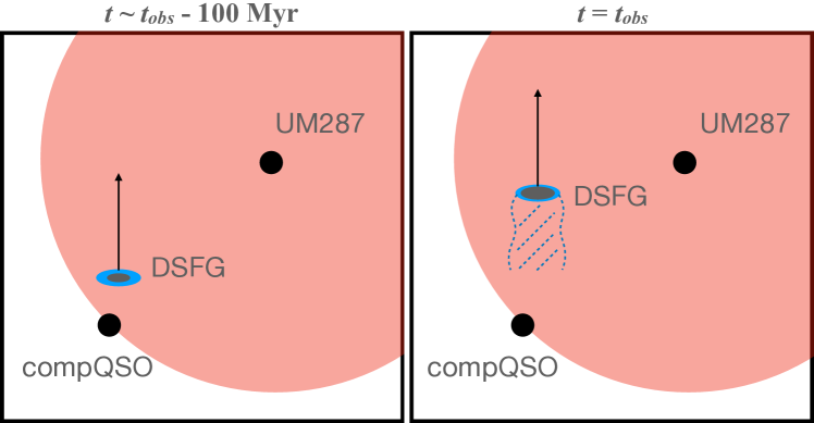 Figure 7: A schematic figure to show the proposed hypothetical scenario regarding the evolution of the newly discovered Slug-DSFG, where in the left shows the Slug-DSFG just entering the halo where gas stripping started to become effective. For simplicity we assume no relative movement between UM287 and the companion quasar. As shown in the right, we suspect that over the past 100 Myr the Slug-DSFG has moved to the north by 100 kpc in projected distance with a projected velocity of 1000 km s-1, in the meantime the stripped gas has been slowly entrained via shocks and gas mixing by the massive (1012-1013 M⊙) hot halo of UM287 and a virial radius of 150 kpc. The Slug-DSFG has also been experiencing strangulation, where the hot halo stops further accretion of cold gas so the gas reservoir has slowly drained out, therefore decreasing both the gas fraction and gas-to-dust ratios.
4.6.3 Slug-DSFG and ram pressure stripping
The newly discovered Slug-DSFG appears to have a velocity consistent with that of the Ly component at km s-1, the region 1 defined in Leibler et al. (2018). Indeed, the slit 2 of our Keck/LRIS spectrum shows that the Slug-DSFG sit at the far end of this Ly filament (Figure 5), suggesting that they belong to the same structure. The fact that we find possible evidence of gas stripping from the Slug-DSFG could further suggest that perhaps the Ly filament is a result of this stripped gas. The smooth velocity gradient from km s-1 to the systemic of UM287 could indicate that the stripped gas by ram pressure is gradually slowed down by the hot gas of the quasar halo as soon as it leaves the Slug-DSFG. The morphology of this stripped gas appears elongated to the north-south direction, with an end-to-end size of about 100 kpc in projected distance. Together with the velocity gradient it could be that the Slug-DSFG have been moving from south to north in the sky while experiencing gas stripping. It is unclear what is the tangential peculiar velocity of the Slug-DSFG, but it would take about a crossing time of 100 Myr to move across 100 kpc assuming a projected velocity of about 1000 km s-1, which is roughly the escape velocity for halos similar to that of UM287 (1013 M⊙; e.g., Miller et al. 2018). The question is then can the stripped gas live for that long? The survivability of cold gas in shocked regions has been a challenging issue to models, mainly due to the fact that cold clouds are destroyed faster than their speed being equalized to the surrounding medium. However, recent theoretical studies tackling the acceleration of cold clouds by hot out-flowing winds have shown that efficient radiative cooling from the mixing gas can prolong the lifetime of clouds via mass accretion, such that the clouds can survive and even grown in mass until they are entrained (Gronke & Oh, 2018, 2020). Based on these models, the time scale, dubbed the drag time , that is required for the clouds with a size of to be accelerated to the velocity of the hot wind , is , where is the overdensity of the cloud compared to the wind which is typically 100-1000. Since the physical processes involved are similar, meaning acceleration (in our case de-acceleration) of cold clouds by surrounding hot gas via shocks and gas mixing, we assume these models to be applicable to the situation of ram pressure stripping discussed here. In such a case would become the peculiar velocity of the Slug-DSFG with respect to the quasar halo. Assuming again the peculiar velocity of 1000 km s-1, =1000, and the size of the giant molecular clouds of pc, as observed by lensed dusty galaxies (Swinbank et al., 2015; Dessauges-Zavadsky et al., 2019), is about 100 Myr. While this remains a zeroth order estimate, as all assumed parameters are not well constrained, it is intriguing that with reasonable assumptions the drag time agrees with the crossing time of Slug-DSFG, supporting the hypothesis of the Ly filament being the stripped gas slowed down by the hot halo gas. Building on these arguments, we can also estimate the amount of gas mass stripped. Following Gunn & Gott (1972), for a galaxy with a stellar surface density and gas surface density and moving with a peculiar velocity with respect to the hot halo of a volume density , ram pressure stripping starts to become efficient once . Hydro-dynamical simulations of 1012 M⊙ halos at , similar to the halo hosting UM287, have shown that cm-3 (Nelson et al., 2016) at about half of the virial radius, based on the projected distance between Slug-DSFG and UM287. For the mass profile of Slug-DSFG, following Section 4.2 we assume an exponential disk profile with a half-light radius of 3 kpc and a gas fraction of 0.2. For a velocity of 1000 km s-1 we find that ram pressure from the hot halo could remove gas of the Slug-DSFG beyond a radius of 9 kpc, and the gas masses stripped is about a few times M⊙, estimated by integrating the gas mass profile beyond this radius. This estimate likely lies in the lower end since the gas fraction was likely to be higher in the beginning when the Slug-DSFG first entered the hot halo, and the volume density could also be higher due to the limited resolution in simulations. If we increase the gas fraction to a typical SMG value of 0.5 and by one order of magnitude the stripped masses would be about 109 M⊙. As a consistency check we can compare this number to that estimated from the Ly filament. Assuming a column density of , which is the median value from absorption studies of quasar halos (Lau et al., 2016), and the area of arcsec2 roughly defined by the ellipse in Figure 6 (and consistent with the extend of emission along slit 2; Figure 5), we obtain a cool gas mass of M⊙, where mp is the proton mass and =0.76 is the hydrogen mass fraction (Pagel, 1997). Even though this value is again a zeroth order estimate, as the column densities inferred from absorption studies have a scatter of 1 dex and the area defined is rough, it is remarkably close to the estimates based on the Slug-DSFG. Interestingly, the amount of stripped gas turns out to be only a few percent of the total gas mass of the Slug-DSFG. So a more likely cause for a lower gas fraction and a lower gas-to-dust ratio for Slug-DSFG, or even UM287, is strangulation, where the gas was mainly consumed by star formation without replenishment from continuous feeding of cold gas. Given the estimated SFR from cigale and the estimated crossing time of 100 Myr, the gas masses consumed by star formation during this time would be about 21010 M⊙, accounting for most of deficit in gas masses when comparing to typical SMGs. To provide a summary of what we have found from the Slug-DSFG, we sketch a schematic picture in Figure 7 to help visualize our proposed hypothesis. We suspect that the Slug-DSFG entered the halo about Myr ago when gas stripping started to become effective, and over the past Myr the Slug-DSFG has moved 100 kpc to the north with a projected velocity of 1000 km -1, leaving behind 108-109 M⊙ stripped gas filaments that emit in Ly (middle panel in Figure 5) which become part of the ELAN and have been slowly entrained to the hot halo via shocks and gas mixing. The Slug-DSFG in the meantime has been experiencing strangulation where the hot halo stop further accretion of cold gas and the Slug-DSFG has consumed 1010 M⊙ via star formation, thus showing a deficit in gas fraction and gas-to-dust ratios (Section 4.2 and Section 4.4).5 Summary
To explore the origin of the enormous Ly nebulae (ELAN), we have started A Multiwavelngth Study of ELAN Environment (AMUSE2; Arrigoni Battaia et al. 2018b, 2021; Nowotka et al. 2021) to measure and quantify the physical properties of sources that are located within or around ELAN. In this third paper of the series, we present single pointing band 4 ALMA CO(4-3) and [CI](1-0) observations toward an ELAN at , dubbed the Slug ELAN (Cantalupo et al., 2014). We summarize the results in the following. 1. We obtain significant detections in 2 mm continuum from three sources and two of which also emit lines. Two of these three detected sources were known previously, UM287 and its companion quasar, and the other is a newly discovered source detected in both continuum and line. Our results are in favor of it being a dusty star-forming galaxy, dubbed Slug-DSFG, located approximately 100 projected kpc south-east of UM287 and sitting within the ELAN with a velocity difference of km s-1 with respect to UM287. 2. With careful modeling of SED and dynamical analyses it is found that while their PDR conditions are similar to other comparison quasar and dusty galaxy samples at similar redshifts in the field, the Slug-DSFG and UM287 appear low in both gas fraction and gas-to-dust ratio, which have also been found on sources in another ELAN (Arrigoni Battaia et al., 2021), suggesting environmental effects from the host massive halos, with estimated masses of M⊙ via various methods. 3. Remarkably, our Keck long-slit spectra taken previously coincidentally covered the Slug-DSFG along with other regions of the nebula, revealing significant Ly emission from the Slug-DSFG, as well as an extending Ly tail toward the south with about 100 kpc in length that connects both in real and velocity spaces with the Slug-DSFG. 4. With simple but realistic assumptions we propose that the Ly tail is a result of stripped gas from the Slug-DSFG, which entered the influence of the hot halo 100 Myr ago and has been moving from south to north on sky with a projected velocity of about 1000 km s-1. The gas mass stripped over this period of time is estimated to be about 109 M⊙, contributing to the dense cold gas reservoir that is believed to be responsible to the exceptional Ly luminosity measured from this ELAN. 5. Under the proposed scenario, the estimated level of the stripped mass suggests that the main cause for the lower gas fraction and gas-to-dust ratio observed in the Slug-DSFG is more likely to be strangulation, where over the last 100 Myr star formation has turned M⊙ of gas to stars without being further replenished, which is the amount comparable to the observed deficit. Assuming the current SFR remains largely unchanged and it is gravitationally bound to the halo, a natural prediction based on this proposed scenario is that the Slug-DSFG will run out of gas, thus quenched, in about 100 Myr. Our results highlight the importance of submillimeter observations of ELAN fields, which complement optical studies on properties of dust and molecular gas and help decipher the origin of ELAN. Last but not least, the estimated stripped gas mass is only about 10% of the total dense and cool gas in the halo inferred from optical studies, which motivates deeper submillimeter observations in order to search for obscured but less massive satellites or companions.References
- Alaghband-Zadeh et al. (2013) Alaghband-Zadeh, S., Chapman, S. C., Swinbank, A. M., et al. 2013, MNRAS, 435, 1493, doi: 10.1093/mnras/stt1390
- Alexander & Hickox (2012) Alexander, D. M., & Hickox, R. C. 2012, New A Rev., 56, 93, doi: 10.1016/j.newar.2011.11.003
- An et al. (2019) An, F. X., Simpson, J. M., Smail, I., et al. 2019, ApJ, 886, 48, doi: 10.3847/1538-4357/ab4d53
- Aravena et al. (2020) Aravena, M., Boogaard, L., Gónzalez-López, J., et al. 2020, ApJ, 901, 79, doi: 10.3847/1538-4357/ab99a2
- Arrigoni Battaia et al. (2015) Arrigoni Battaia, F., Hennawi, J. F., Prochaska, J. X., & Cantalupo, S. 2015, ApJ, 809, 163, doi: 10.1088/0004-637X/809/2/163
- Arrigoni Battaia et al. (2018a) Arrigoni Battaia, F., Prochaska, J. X., Hennawi, J. F., et al. 2018a, MNRAS, 473, 3907, doi: 10.1093/mnras/stx2465
- Arrigoni Battaia et al. (2018b) Arrigoni Battaia, F., Chen, C.-C., Fumagalli, M., et al. 2018b, A&A, 620, A202, doi: 10.1051/0004-6361/201834195
- Arrigoni Battaia et al. (2021) Arrigoni Battaia, F., Chen, C.-C., Liu, H.-Y. B., et al. 2021, A&A submitted
- Astropy Collaboration et al. (2013) Astropy Collaboration, Robitaille, T. P., Tollerud, E. J., et al. 2013, A&A, 558, A33, doi: 10.1051/0004-6361/201322068
- Badole et al. (2020) Badole, S., Jackson, N., Hartley, P., et al. 2020, MNRAS, 496, 138, doi: 10.1093/mnras/staa1488
- Banerji et al. (2017) Banerji, M., Carilli, C. L., Jones, G., et al. 2017, MNRAS, 465, 4390, doi: 10.1093/mnras/stw3019
- Beelen et al. (2006) Beelen, A., Cox, P., Benford, D. J., et al. 2006, ApJ, 642, 694, doi: 10.1086/500636
- Bell et al. (2003) Bell, E. F., McIntosh, D. H., Katz, N., & Weinberg, M. D. 2003, ApJS, 149, 289, doi: 10.1086/378847
- Bertin & Arnouts (1996) Bertin, E., & Arnouts, S. 1996, A&AS, 117, 393
- Bianchi et al. (2017) Bianchi, L., Shiao, B., & Thilker, D. 2017, ApJS, 230, 24, doi: 10.3847/1538-4365/aa7053
- Binney & Tremaine (2008) Binney, J., & Tremaine, S. 2008, Galactic Dynamics: Second Edition
- Birkin et al. (2021) Birkin, J. E., Weiss, A., Wardlow, J. L., et al. 2021, MNRAS, 501, 3926, doi: 10.1093/mnras/staa3862
- Bischetti et al. (2021) Bischetti, M., Feruglio, C., Piconcelli, E., et al. 2021, A&A, 645, A33, doi: 10.1051/0004-6361/202039057
- Boogaard et al. (2020) Boogaard, L. A., van der Werf, P., Weiss, A., et al. 2020, ApJ, 902, 109, doi: 10.3847/1538-4357/abb82f
- Boquien et al. (2019) Boquien, M., Burgarella, D., Roehlly, Y., et al. 2019, A&A, 622, A103, doi: 10.1051/0004-6361/201834156
- Bothwell et al. (2013) Bothwell, M. S., Smail, I., Chapman, S. C., et al. 2013, MNRAS, 429, 3047
- Bothwell et al. (2017) Bothwell, M. S., Aguirre, J. E., Aravena, M., et al. 2017, MNRAS, 466, 2825, doi: 10.1093/mnras/stw3270
- Bourne et al. (2019) Bourne, N., Dunlop, J. S., Simpson, J. M., et al. 2019, MNRAS, 482, 3135, doi: 10.1093/mnras/sty2773
- Brisbin et al. (2019) Brisbin, D., Aravena, M., Daddi, E., et al. 2019, A&A, 628, A104, doi: 10.1051/0004-6361/201935148
- Bruzual & Charlot (2003) Bruzual, G., & Charlot, S. 2003, MNRAS, 344, 1000, doi: 10.1046/j.1365-8711.2003.06897.x
- Cai et al. (2017) Cai, Z., Fan, X., Yang, Y., et al. 2017, ApJ, 837, 71, doi: 10.3847/1538-4357/aa5d14
- Cai et al. (2018) Cai, Z., Hamden, E., Matuszewski, M., et al. 2018, ApJ, 861, L3, doi: 10.3847/2041-8213/aacce6
- Cai et al. (2019) Cai, Z., Cantalupo, S., Prochaska, J. X., et al. 2019, ApJS, 245, 23, doi: 10.3847/1538-4365/ab4796
- Calistro Rivera et al. (2018) Calistro Rivera, G., Hodge, J. A., Smail, I., et al. 2018, ApJ, 863, 56, doi: 10.3847/1538-4357/aacffa
- Calzetti et al. (2000) Calzetti, D., Armus, L., Bohlin, R. C., et al. 2000, ApJ, 533, 682, doi: 10.1086/308692
- Cantalupo et al. (2014) Cantalupo, S., Arrigoni-Battaia, F., Prochaska, J. X., Hennawi, J. F., & Madau, P. 2014, Nature, 506, 63, doi: 10.1038/nature12898
- Cantalupo et al. (2019) Cantalupo, S., Pezzulli, G., Lilly, S. J., et al. 2019, MNRAS, 483, 5188, doi: 10.1093/mnras/sty3481
- Carilli & Walter (2013) Carilli, C. L., & Walter, F. 2013, ARA&A, 51, 105, doi: 10.1146/annurev-astro-082812-140953
- Casali et al. (2006) Casali, M., Pirard, J.-F., Kissler-Patig, M., et al. 2006, in Society of Photo-Optical Instrumentation Engineers (SPIE) Conference Series, Vol. 6269, Society of Photo-Optical Instrumentation Engineers (SPIE) Conference Series, ed. I. S. McLean & M. Iye, 62690W, doi: 10.1117/12.670150
- Chabrier (2003) Chabrier, G. 2003, PASP, 115, 763, doi: 10.1086/376392
- Chen et al. (2015) Chen, C.-C., Smail, I., Swinbank, A. M., et al. 2015, ApJ, 799, 194, doi: 10.1088/0004-637X/799/2/194
- Chen et al. (2016a) —. 2016a, ApJ, 831, 91, doi: 10.3847/0004-637X/831/1/91
- Chen et al. (2016b) Chen, C.-C., Smail, I., Ivison, R. J., et al. 2016b, ApJ, 820, 82, doi: 10.3847/0004-637X/820/2/82
- Chen et al. (2017) Chen, C.-C., Hodge, J. A., Smail, I., et al. 2017, ApJ, 846, 108, doi: 10.3847/1538-4357/aa863a
- Condon et al. (1998) Condon, J. J., Cotton, W. D., Greisen, E. W., et al. 1998, AJ, 115, 1693, doi: 10.1086/300337
- da Cunha et al. (2008) da Cunha, E., Charlot, S., & Elbaz, D. 2008, MNRAS, 388, 1595, doi: 10.1111/j.1365-2966.2008.13535.x
- Dannerbauer et al. (2014) Dannerbauer, H., Kurk, J. D., De Breuck, C., et al. 2014, A&A, 570, A55, doi: 10.1051/0004-6361/201423771
- de Blok & Walter (2014) de Blok, W. J. G., & Walter, F. 2014, AJ, 147, 96, doi: 10.1088/0004-6256/147/5/96
- De Vis et al. (2019) De Vis, P., Jones, A., Viaene, S., et al. 2019, A&A, 623, A5, doi: 10.1051/0004-6361/201834444
- Decarli et al. (2021) Decarli, R., Arrigoni-Battaia, F., Hennawi, J. F., et al. 2021, A&A, 645, L3, doi: 10.1051/0004-6361/202039814
- Decarli et al. (2018) Decarli, R., Walter, F., Venemans, B. P., et al. 2018, ApJ, 854, 97, doi: 10.3847/1538-4357/aaa5aa
- Dekel & Birnboim (2006) Dekel, A., & Birnboim, Y. 2006, MNRAS, 368, 2, doi: 10.1111/j.1365-2966.2006.10145.x
- Delvecchio et al. (2014) Delvecchio, I., Gruppioni, C., Pozzi, F., et al. 2014, MNRAS, 439, 2736, doi: 10.1093/mnras/stu130
- Dessauges-Zavadsky et al. (2019) Dessauges-Zavadsky, M., Richard, J., Combes, F., et al. 2019, Nature Astronomy, 3, 1115, doi: 10.1038/s41550-019-0874-0
- Draine & Li (2007) Draine, B. T., & Li, A. 2007, ApJ, 657, 810, doi: 10.1086/511055
- Draine et al. (2014) Draine, B. T., Aniano, G., Krause, O., et al. 2014, ApJ, 780, 172, doi: 10.1088/0004-637X/780/2/172
- Dressler (1980) Dressler, A. 1980, ApJ, 236, 351, doi: 10.1086/157753
- Dudzevičiūtė et al. (2020) Dudzevičiūtė, U., Smail, I., Swinbank, A. M., et al. 2020, MNRAS, 494, 3828, doi: 10.1093/mnras/staa769
- Eftekharzadeh et al. (2015) Eftekharzadeh, S., Myers, A. D., White, M., et al. 2015, MNRAS, 453, 2779, doi: 10.1093/mnras/stv1763
- Emonts et al. (2019) Emonts, B. H. C., Cai, Z., Prochaska, J. X., Li, Q., & Lehnert, M. D. 2019, ApJ, 887, 86, doi: 10.3847/1538-4357/ab45f4
- Emonts et al. (2015) Emonts, B. H. C., De Breuck, C., Lehnert, M. D., et al. 2015, A&A, 584, A99, doi: 10.1051/0004-6361/201526090
- Fogasy et al. (2020) Fogasy, J., Knudsen, K. K., Drouart, G., Lagos, C. D. P., & Fan, L. 2020, MNRAS, 493, 3744, doi: 10.1093/mnras/staa472
- Fossati et al. (2021) Fossati, M., Fumagalli, M., Lofthouse, E. K., et al. 2021, MNRAS, 503, 3044, doi: 10.1093/mnras/stab660
- Fritz et al. (2006) Fritz, J., Franceschini, A., & Hatziminaoglou, E. 2006, MNRAS, 366, 767, doi: 10.1111/j.1365-2966.2006.09866.x
- Genzel et al. (2020) Genzel, R., Price, S. H., Übler, H., et al. 2020, ApJ, 902, 98, doi: 10.3847/1538-4357/abb0ea
- González-López et al. (2017) González-López, J., Bauer, F. E., Aravena, M., et al. 2017, A&A, 608, A138, doi: 10.1051/0004-6361/201730961
- González-López et al. (2019) González-López, J., Decarli, R., Pavesi, R., et al. 2019, ApJ in press, arXiv:1903.09161. https://arxiv.org/abs/1903.09161
- González-López et al. (2020) González-López, J., Novak, M., Decarli, R., et al. 2020, ApJ, 897, 91, doi: 10.3847/1538-4357/ab765b
- Gronke & Oh (2018) Gronke, M., & Oh, S. P. 2018, MNRAS, 480, L111, doi: 10.1093/mnrasl/sly131
- Gronke & Oh (2020) —. 2020, MNRAS, 492, 1970, doi: 10.1093/mnras/stz3332
- Gullberg et al. (2016) Gullberg, B., Lehnert, M. D., De Breuck, C., et al. 2016, A&A, 591, A73, doi: 10.1051/0004-6361/201527647
- Gunn & Gott (1972) Gunn, J. E., & Gott, J. Richard, I. 1972, ApJ, 176, 1, doi: 10.1086/151605
- Hennawi et al. (2015) Hennawi, J. F., Prochaska, J. X., Cantalupo, S., & Arrigoni-Battaia, F. 2015, Science, 348, 779, doi: 10.1126/science.aaa5397
- Henry et al. (2015) Henry, A., Scarlata, C., Martin, C. L., & Erb, D. 2015, ApJ, 809, 19, doi: 10.1088/0004-637X/809/1/19
- Hickox et al. (2012) Hickox, R. C., Wardlow, J. L., Smail, I., et al. 2012, MNRAS, 421, 284
- Hill et al. (2019) Hill, R., Chapman, S. C., Scott, D., et al. 2019, MNRAS, 485, 753, doi: 10.1093/mnras/stz429
- Hirashita (1999) Hirashita, H. 1999, ApJ, 510, L99, doi: 10.1086/311806
- Holland et al. (2013) Holland, W. S., Bintley, D., Chapin, E. L., et al. 2013, MNRAS, 2513. https://arxiv.org/abs/1301.3650
- Hopkins et al. (2006) Hopkins, P. F., Hernquist, L., Cox, T. J., et al. 2006, ApJS, 163, 1, doi: 10.1086/499298
- Hopkins et al. (2007) Hopkins, P. F., Richards, G. T., & Hernquist, L. 2007, ApJ, 654, 731, doi: 10.1086/509629
- Ivison et al. (2012) Ivison, R. J., Smail, I., Amblard, A., et al. 2012, MNRAS, 425, 1320, doi: 10.1111/j.1365-2966.2012.21544.x
- Kamenetzky et al. (2016) Kamenetzky, J., Rangwala, N., Glenn, J., Maloney, P. R., & Conley, A. 2016, ApJ, 829, 93, doi: 10.3847/0004-637X/829/2/93
- Kaufman et al. (2006) Kaufman, M. J., Wolfire, M. G., & Hollenbach, D. J. 2006, ApJ, 644, 283, doi: 10.1086/503596
- Kaufman et al. (1999) Kaufman, M. J., Wolfire, M. G., Hollenbach, D. J., & Luhman, M. L. 1999, ApJ, 527, 795, doi: 10.1086/308102
- Kelvin et al. (2014) Kelvin, L. S., Driver, S. P., Robotham, A. S. G., et al. 2014, MNRAS, 444, 1647, doi: 10.1093/mnras/stu1507
- Kennicutt & Evans (2012) Kennicutt, R. C., & Evans, N. J. 2012, ARA&A, 50, 531, doi: 10.1146/annurev-astro-081811-125610
- Lau et al. (2016) Lau, M. W., Prochaska, J. X., & Hennawi, J. F. 2016, ApJS, 226, 25, doi: 10.3847/0067-0049/226/2/25
- Leibler et al. (2018) Leibler, C. N., Cantalupo, S., Holden, B. P., & Madau, P. 2018, MNRAS, 480, 2094, doi: 10.1093/mnras/sty1764
- Leitherer et al. (2002) Leitherer, C., Li, I. H., Calzetti, D., & Heckman, T. M. 2002, ApJS, 140, 303, doi: 10.1086/342486
- Leroy et al. (2011) Leroy, A. K., Bolatto, A., Gordon, K., et al. 2011, ApJ, 737, 12, doi: 10.1088/0004-637X/737/1/12
- Lilly et al. (1999) Lilly, S. J., Eales, S. A., Gear, W. K. P., et al. 1999, ApJ, 518, 641, doi: 10.1086/307310
- Lim et al. (2020) Lim, C.-F., Chen, C.-C., Smail, I., et al. 2020, ApJ, 895, 104, doi: 10.3847/1538-4357/ab8eaf
- Madau & Dickinson (2014) Madau, P., & Dickinson, M. 2014, ARA&A, 52, 415, doi: 10.1146/annurev-astro-081811-125615
- Magdis et al. (2012) Magdis, G. E., Daddi, E., Béthermin, M., et al. 2012, ApJ, 760, 6, doi: 10.1088/0004-637X/760/1/6
- Man et al. (2019) Man, A. W. S., Lehnert, M. D., Vernet, J. D. R., De Breuck, C., & Falkendal, T. 2019, A&A, 624, A81, doi: 10.1051/0004-6361/201834542
- Martí-Vidal et al. (2014) Martí-Vidal, I., Vlemmings, W. H. T., Muller, S., & Casey, S. 2014, A&A, 563, A136, doi: 10.1051/0004-6361/201322633
- Martin et al. (2015) Martin, D. C., Matuszewski, M., Morrissey, P., et al. 2015, Nature, 524, 192, doi: 10.1038/nature14616
- McIntosh et al. (1999) McIntosh, D. H., Rieke, M. J., Rix, H. W., Foltz, C. B., & Weymann, R. J. 1999, ApJ, 514, 40, doi: 10.1086/306936
- Meiksin (2006) Meiksin, A. 2006, MNRAS, 365, 807, doi: 10.1111/j.1365-2966.2005.09756.x
- Miller et al. (2018) Miller, T. B., Chapman, S. C., Aravena, M., et al. 2018, Nature, 556, 469, doi: 10.1038/s41586-018-0025-2
- Moffett et al. (2016) Moffett, A. J., Ingarfield, S. A., Driver, S. P., et al. 2016, MNRAS, 457, 1308, doi: 10.1093/mnras/stv2883
- Moster et al. (2018) Moster, B. P., Naab, T., & White, S. D. M. 2018, MNRAS, 477, 1822, doi: 10.1093/mnras/sty655
- Myers et al. (2006) Myers, A. D., Brunner, R. J., Richards, G. T., et al. 2006, ApJ, 638, 622, doi: 10.1086/499093
- Narayanan et al. (2010) Narayanan, D., Hayward, C. C., Cox, T. J., et al. 2010, MNRAS, 401, 1613
- Navarro et al. (1997) Navarro, J. F., Frenk, C. S., & White, S. D. M. 1997, ApJ, 490, 493, doi: 10.1086/304888
- Nelson et al. (2016) Nelson, D., Genel, S., Pillepich, A., et al. 2016, MNRAS, 460, 2881, doi: 10.1093/mnras/stw1191
- Nowotka et al. (2021) Nowotka, M., Chen, C.-C., Arrigoni Battaia, F., et al. 2021, A&A submitted
- Oke & Gunn (1983) Oke, J. B., & Gunn, J. E. 1983, ApJ, 266, 713, doi: 10.1086/160817
- Oke et al. (1995) Oke, J. B., Cohen, J. G., Carr, M., et al. 1995, PASP, 107, 375, doi: 10.1086/133562
- Ouchi et al. (2020) Ouchi, M., Ono, Y., & Shibuya, T. 2020, Annual Review of Astronomy and Astrophysics, 58, 617, doi: 10.1146/annurev-astro-032620-021859
- Pagel (1997) Pagel, B. E. J. 1997, Nucleosynthesis and Chemical Evolution of Galaxies
- Papadopoulos et al. (2004) Papadopoulos, P. P., Thi, W. F., & Viti, S. 2004, MNRAS, 351, 147, doi: 10.1111/j.1365-2966.2004.07762.x
- Pâris et al. (2017) Pâris, I., Petitjean, P., Ross, N. P., et al. 2017, A&A, 597, A79, doi: 10.1051/0004-6361/201527999
- Pavesi et al. (2018) Pavesi, R., Sharon, C. E., Riechers, D. A., et al. 2018, ApJ, 864, 49, doi: 10.3847/1538-4357/aacb79
- Peng et al. (2015) Peng, Y., Maiolino, R., & Cochrane, R. 2015, Nature, 521, 192, doi: 10.1038/nature14439
- Pensabene et al. (2021) Pensabene, A., Decarli, R., Bañados, E., et al. 2021, arXiv e-prints, arXiv:2105.09958. https://arxiv.org/abs/2105.09958
- Perna et al. (2018) Perna, M., Sargent, M. T., Brusa, M., et al. 2018, A&A, 619, A90, doi: 10.1051/0004-6361/201833040
- Planck Collaboration et al. (2014) Planck Collaboration, Ade, P. A. R., Aghanim, N., et al. 2014, A&A, 571, A16, doi: 10.1051/0004-6361/201321591
- Porciani & Norberg (2006) Porciani, C., & Norberg, P. 2006, MNRAS, 371, 1824, doi: 10.1111/j.1365-2966.2006.10813.x
- Pound & Wolfire (2008) Pound, M. W., & Wolfire, M. G. 2008, in Astronomical Society of the Pacific Conference Series, Vol. 394, Astronomical Data Analysis Software and Systems XVII, ed. R. W. Argyle, P. S. Bunclark, & J. R. Lewis, 654
- Rigby et al. (2014) Rigby, E. E., Hatch, N. A., Röttgering, H. J. A., et al. 2014, MNRAS, 437, 1882, doi: 10.1093/mnras/stt2019
- Rodríguez-Torres et al. (2017) Rodríguez-Torres, S. A., Comparat, J., Prada, F., et al. 2017, MNRAS, 468, 728, doi: 10.1093/mnras/stx454
- Shapley et al. (2020) Shapley, A. E., Cullen, F., Dunlop, J. S., et al. 2020, ApJ, 903, L16, doi: 10.3847/2041-8213/abc006
- Shen et al. (2007) Shen, Y., Strauss, M. A., Oguri, M., et al. 2007, AJ, 133, 2222. http://stacks.iop.org/1538-3881/133/i=5/a=2222
- Solomon & Vanden Bout (2005) Solomon, P. M., & Vanden Bout, P. A. 2005, ARA&A, 43, 677, doi: 10.1146/annurev.astro.43.051804.102221
- Stacey et al. (2018) Stacey, H. R., McKean, J. P., Robertson, N. C., et al. 2018, MNRAS, 476, 5075, doi: 10.1093/mnras/sty458
- Stach et al. (2021) Stach, S. M., Smail, I., Amvrosiadis, A., et al. 2021, MNRAS, doi: 10.1093/mnras/stab714
- Stevens et al. (2003) Stevens, J. A., Ivison, R. J., Dunlop, J. S., et al. 2003, Nature, 425, 264
- Stewart et al. (2011) Stewart, K. R., Kaufmann, T., Bullock, J. S., et al. 2011, ApJ, 738, 39, doi: 10.1088/0004-637X/738/1/39
- Swinbank et al. (2015) Swinbank, A. M., Dye, S., Nightingale, J. W., et al. 2015, ApJ, 806, L17, doi: 10.1088/2041-8205/806/1/L17
- Tacconi et al. (2008) Tacconi, L. J., Genzel, R., Smail, I., et al. 2008, ApJ, 680, 246, doi: 10.1086/587168
- Tadaki et al. (2019) Tadaki, K.-i., Iono, D., Hatsukade, B., et al. 2019, ApJ in press. https://arxiv.org/abs/1903.11234
- Tempel et al. (2014) Tempel, E., Tamm, A., Gramann, M., et al. 2014, A&A, 566, A1, doi: 10.1051/0004-6361/201423585
- Thomas et al. (2010) Thomas, D., Maraston, C., Schawinski, K., Sarzi, M., & Silk, J. 2010, MNRAS, 404, 1775, doi: 10.1111/j.1365-2966.2010.16427.x
- Tielens & Hollenbach (1985) Tielens, A. G. G. M., & Hollenbach, D. 1985, ApJ, 291, 722, doi: 10.1086/163111
- Toft et al. (2014) Toft, S., Smolčić, V., Magnelli, B., et al. 2014, ApJ, 782, 68, doi: 10.1088/0004-637X/782/2/68
- Trakhtenbrot et al. (2017) Trakhtenbrot, B., Lira, P., Netzer, H., et al. 2017, ApJ, 836, 8, doi: 10.3847/1538-4357/836/1/8
- Tuan-Anh et al. (2017) Tuan-Anh, P., Hoai, D. T., Nhung, P. T., et al. 2017, MNRAS, 467, 3513, doi: 10.1093/mnras/stx212
- Uzgil et al. (2016) Uzgil, B. D., Bradford, C. M., Hailey-Dunsheath, S., Maloney, P. R., & Aguirre, J. E. 2016, ApJ, 832, 209, doi: 10.3847/0004-637X/832/2/209
- Valentino et al. (2018) Valentino, F., Magdis, G. E., Daddi, E., et al. 2018, ApJ, 869, 27, doi: 10.3847/1538-4357/aaeb88
- Valentino et al. (2020) —. 2020, ApJ, 890, 24, doi: 10.3847/1538-4357/ab6603
- Walter et al. (2016) Walter, F., Decarli, R., Aravena, M., et al. 2016, ApJ, 833, 67, doi: 10.3847/1538-4357/833/1/67
- Wang et al. (2015) Wang, L., Viero, M., Ross, N. P., et al. 2015, MNRAS, 449, 4476, doi: 10.1093/mnras/stv559
- Weiß et al. (2003) Weiß, A., Henkel, C., Downes, D., & Walter, F. 2003, A&A, 409, L41, doi: 10.1051/0004-6361:20031337
- Wilkinson et al. (2017) Wilkinson, A., Almaini, O., Chen, C.-C., et al. 2017, MNRAS, 464, 1380, doi: 10.1093/mnras/stw2405
- Wright et al. (2010) Wright, E. L., Eisenhardt, P. R. M., Mainzer, A. K., et al. 2010, The Astronomical Journal, 140, 1868, doi: 10.1088/0004-6256/140/6/1868
- Zeballos et al. (2018) Zeballos, M., Aretxaga, I., Hughes, D. H., et al. 2018, MNRAS, 479, 4577, doi: 10.1093/mnras/sty1714
Abstract
We present ALMA observations on and around the radio-quiet quasar UM287 at . Together with a companion quasar, UM287 is believed to play a major role in powering the surrounding enormous Ly nebula (ELAN), dubbed the Slug ELAN, that has an end-to-end size of 450 physical kpc. In addition to the quasars, we detect a new dusty star-forming galaxy (DSFG), dubbed the Slug-DSFG, in 2 mm continuum with a single emission line consistent with CO(4-3). The Slug-DSFG sits at a projected distance of 100 kpc south-east from UM287, with a systemic velocity difference of km s-1 with respect to UM287, suggesting it being a possible contributor to the powering of the Slug ELAN. With careful modeling of SED and dynamical analyses it is found that the Slug-DSFG and UM287 appear low in both gas fraction and gas-to-dust ratio, suggesting environmental effects due to the host massive halo. In addition, our Keck long-slit spectra reveal significant Ly emissions from the Slug-DSFG, as well as a Ly tail that starts at the location and velocity of the Slug-DSFG and extends towards the south, with a projected length of about 100 kpc. Supported by various analytical estimates we propose that the Ly tail is a result of the Slug-DSFG experiencing ram pressure stripping. The gas mass stripped is estimated to be about 109 M⊙, contributing to the dense warm/cool gas reservoir that is believed to help power the exceptional Ly luminosity.