Polaronic effects induced by non-equilibrium vibrons in a single-molecule transistor

Abstract

Current-voltage characteristics of a single-electron transistor with a vibrating quantum dot were calculated assuming vibrons to be in a coherent (non-equilibrium) state. For a large amplitude of quantum dot oscillations we predict strong suppression of conductance and the lifting of polaronic blockade by bias voltage in the form of steps in $I-V$ curves. The height of the steps differs from the prediction of the Franck-Condon theory (valid for equilibrated vibrons) and the current saturates at lower voltages then for the case, when vibrons are in equilibrium state.

I Introduction

Tunneling spectroscopy is a well-known method to study of electron-phonon interaction in bulk metals (see e.g. Ref.Yanson1 ). Electron transport spectroscopy can be used for studying of vibration properties of molecules in single-molecule-based transistors McEuen ; Utko . Current-voltage characteristics of single electron transistors (SETs), where fullerene molecule McEuen , suspended single-wall carbon nanotube van der Zant ; Leturcq ; babic or carbon nano-peapod Utko are used as a base element, demonstrate at low temperatures additional sharp features (steps) at bias voltages $eV_{n}\simeq n\hbar\omega$ ($\omega$ is the angular frequency of vibrational degree of freedom). The simplest models (see e.g. review Ref.krivepalevskij ) that describe step-like behavior of $I-V$ curves are based, as a rule, on a theory where phonon excitations are dispersion-less (vibrons with a single frequency) and they are assumed to be in equilibrium with the heat bath at temperature $T$ (bulk metallic electrodes can play the role of this heat bath). Steps in current-voltage dependencies (equidistant peaks in differential conductance) are associated with the opening of inelastic channels of electron tunneling through vibrating quantum dot. For strong electron-vibron interaction these models predict: (i) Franck-Condon blockade von Oppen (exponential suppression) of conductance at low temperatures $T\ll\hbar\omega$ , and (ii) non-monotonous temperature dependence of conductance. All these effects were observed in experiments McEuen ; Utko .

When coupling of vibron subsystem to the heat bath is weak and vibrons are not in equilibrium during the time of electron tunneling through the system, their density matrix can not be in the Gibbs form and it has to be evaluated from the solution of kinetic equations. This problem can be solved only numerically (see e.g.kinaret ). There are only few papers mitra ; kit ; kit2 , where vibrons in electron transport in SET were considered as non-equilibrated. In Ref.kit it was assumed that vibron subsystem is in a coherent state. In the approach used in the cited paper, the density matrix of coherent state was time-independent, that contradicts Liuville-von Neumann equation for density matrix of noninteracting vibrons. Therefore the results of this approach are questionable and the problem of electron transport through a vibrating quantum dot with coherent vibrons has to be re-examined.

In our paper we consider single-electron transistor with vibrating quantum dot, where vibronic subsystem is described by time- dependent density matrix. Physically this approach corresponds to coherent oscillations of quantum dot treated as harmonic quantum oscillator. Coherent states of harmonic oscillators are well known in physics (see e.g. Refscoh ). In tunnel electron transport they are appeared, for instance, in weak superconductivity (Josephson current through a vibrating quantum dot, see Ref.Zazunov and referencies therein). Last years coherent states of photons (”Schroedinger cat” states) coupled to qubits and qubits formed by the coherent photon states became a hot topic of studies in quantum computing science (see e.g. review Ref.Girvin ).

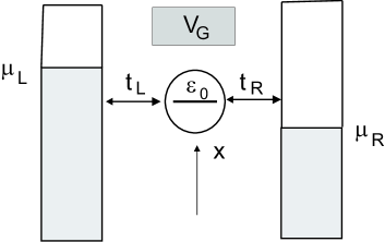
Figure 1: Sketch of the single-electron transistor. A vibrating one-level ($\varepsilon_{0}$ is the level energy) quantum dot (macromolecule) is placed between two bulk electrodes biased by the voltage $V$. The dot tunnel couples ($t_{L}=t_{R}=t_{0}$ is the tunneling amplitude) to the leads with the chemical potentials $\mu_{L,R},\;\mu_{L}-\mu_{R}=eV$ and the temperature $T$. The gate voltage $V_{G}$ is set $\varepsilon_{0}(V_{G})=\varepsilon_{F}$, where $\varepsilon_{F}$ is the Fermi energy, to get maximal current. The dot oscillates in $x$ direction perpendicular to the electric current flow. QD oscillations are modelled by the coherent state of one dimensional harmonic oscillator.

The model device we are interesting in is depicted in Fig.1. It consist of two bulk electrodes, source (Left) and drain (Right) leads, with chemical potential biased by voltage $\mu_{L}-\mu_{R}=eV$ and a single level quantum dot (QD), which oscillates in the direction (”$x$”) perpendicular to the direction of electron current flow. Gate voltage, $V_{G}$, is adjusted to maximum tunnel current $\varepsilon_{0}(V_{G})=\varepsilon_{F}$, where $\varepsilon_{0}(V_{G})$ is the dot level energy and $\varepsilon_{F}$ is the Fermi energy of the leads. For simplicity we consider tunneling of spinless electrons in a symmetric junction and it is assumed that the vibration of QD does not change tunneling matrix elements $t_{L}=t_{R}=t_{0}$ . In our paper we consider the process of sequential electron tunneling, when $\max(eV,T)\gg\Gamma$, where $\Gamma\propto|t_{0}|^{2}$ is the level width (characteristic energy of tunnel coupling dot-leads). Our model device can simulate , for instance, SET based on a suspended single-wall carbon nanotube.

We use density matrix approach to calculate periodic in time current through the device (the period $T_{0}=2\pi/\omega$ is determined by the angular frequency $\omega$ of QD oscillations). In order to calculate current-voltage dependencies, we numerically average the current over $T_{0}$. It is shown that the zeroth-harmonic (time-independent) contribution dominates in the Fourier series for the current. Therefore a simple analytic equation for dc electric current (analogous to the current through vibrating QD with equilibrated vibrons) is presented. This formula agrees with our numerical calculation with a high accuracy.

We show that $I-V$ characteristics of a single-electron transistor with coherent vibrons are a step-like function of bias voltage and they do not depend on the phase of coherent state parameter. At large amplitudes of dot oscillations the conductance is strongly suppressed (”polaronic blockade”) regardless the strength of electron-vibron interaction. The heights of the steps and the characteristic voltage of current saturation strongly differ from the prediction the Franck-Condon theory. In particularly the lifting of polaronic blockade occurs at lower voltages than the lifting of Franck-Condon blockade.

II Hamiltonian and equation for density matrix

The Hamiltonian of the system (see schematic picture of our device, Fig.1) consists of four terms,

$$H=H_{l}+H_{dot}+H_{v-d}+H_{tun},$$ (1)

where $H_{l},H_{dot}$ are the Hamiltonians of the non-interacting electrons in the leads and the dot correspondingly,

$$H_{l}=\sum_{k,\kappa}\varepsilon_{k,\kappa}a^{\dagger}_{k,\kappa}a_{k,\kappa},\,H_{dot}=\varepsilon_{0}c^{\dagger}c,$$ (2)

$a_{k,\kappa}^{\dagger}(a_{k,\kappa})$ is the creation (annihilation) operator (with standard anti-commutation relations) of electron in the lead $\kappa=L,R$ with momentum $k$ and energy $\varepsilon_{k,\kappa}$ , $c^{\dagger}(c)$ is the creation (annihilation) operator of electron state in the dot with the energy $\varepsilon_{0}$.

Hamiltonian $H_{v-d}$ describes the vibronic subsystem and the interaction between electrons and vibrons,

$$\hat{H}_{v-d}=\frac{p^{2}}{2m}+\frac{m\omega^{2}x^{2}}{2}+\Delta xc^{\dagger}c.$$ (3)

In Eq.(3) $x,p$ are the canonical conjugating operators of coordinate and momentum, $[x,p]=\imath\hbar,\,\omega,m$ are the frequency of dot oscillations and the mass of the dot, $\Delta$ is the electron-vibron coupling constant.

The Hamiltonian $H_{tun}$ describes the tunnelling of electrons between the dot and the leads and it takes the standard form,

$$H_{tun}=\sum_{k,\kappa}t_{\kappa}a^{\dagger}_{k,\kappa}c+\text{H.c.},$$ (4)

where $t_{\kappa}$ is the tunnelling amplitude. In what follows we restrict ourselves to the symmetric case, $t_{L}=t_{R}=t_{0}$.

It is convenient to perform the unitary transformation, $UHU^{\dagger}\rightarrow H$, with $U=\exp[i\lambda pc^{\dagger}c]$ and $\lambda=\Delta/\hbar m\omega^{2}$. After this transformation the dot-vibron Hamiltonian $H_{v-d}$ (Eq. (3)) takes the diagonal form,

$$H_{v-d}\rightarrow H_{v}=\frac{p^{2}}{2m}+\frac{m\omega^{2}x^{2}}{2},$$ (5)

while the tunnelling Hamiltonian, $H_{tun}$, is transformed to the equation,

$$H_{tun}\rightarrow H_{tun}=t_{0}\sum_{k,\kappa}\text{e}^{-\imath\lambda p}a^{\dagger}_{k,\kappa}c+\text{H.c.}.$$ (6)

The quantum consideration of electron-vibron interacting system is based in what follows on the approximation that the density matrix of the system is factorized to direct product of the leads equilibrium density matrix, the vibron density matrix and the density matrix of the dot,

$$\rho\approx\rho_{l}\otimes\rho_{v}\otimes\rho_{dot}.$$ (7)

This approximation corresponds to the case of sequential electron tunneling, which holds when $\text{max}\{eV,T\}\gg\Gamma$, where $\Gamma$ is the electron level width, $T$ is the temperature and $V$ is the biased voltage. In contrast to the previous works (see e.g. Refs.krivepalevskij ; Shkop ) we will consider non-equilibrated vibrons. Here we assume that they are described by a time-dependent coherent state $|z(t)\rangle$. Note, that in Ref.kit current-voltage characteristics of a single-electron transistor were calculated for time-independent coherent state of vibrons. This assupmtion contradicts to equation of motion of noninteracting vibrons in our model, where $|z(t)\rangle=\exp\left(-\imath H_{v}t\right)|z\rangle,(\hbar=1)$. Here $|z\rangle$ is the eigenfunction of vibron annihilation operator $b,b|z\rangle=z|z\rangle$ ($z$ is the complex number). The corresponding density matrix takes the standard form

$$\rho_{v}(t)=|z(t)\rangle\langle z(t)|.$$ (8)

The Liouville-von Neumann equation for the density matrix

$$\frac{\partial\rho}{\partial t}+\imath[H_{0}+H_{tun},\rho]=0,$$ (9)

where $H_{0}=H_{l}+H_{v}+H_{dot}$, has the formal solution,

$$\rho(t)=\rho(-\infty)-\imath\int_{-\infty}^{t}dt^{\prime}\text{e}^{-\imath H_{0}(t-t^{\prime})}[H_{tun},\rho(t^{\prime})]\text{e}^{\imath H_{0}(t-t^{\prime})}.$$ (10)

After substitution of Eqs.(7), (10) into Eqn.(9) and tracing out both the electronic degrees of freedom of the leads and vibronic degrees of freedom of the dot one gets

$$\frac{\partial\rho_{dot}}{\partial t}+\imath[H_{dot},\rho_{dot}]=$$ (11)

$$-\text{Tr}\int_{-\infty}^{t}dt^{\prime}[H_{tun},\text{e}^{-\imath H_{0}(t-t^{\prime})}[H_{tun},\rho(t^{\prime})]\text{e}^{\imath H_{0}(t-t^{\prime})}].$$

Now we can explicitly calculate averages of electronic and vibronic operators in our approximation of the factorized density matrix Eq.(7). For equilibrium density matrix of electrons in the leads we use the standard expression

$$\langle a^{\dagger}_{k,\kappa}a_{k^{\prime},\kappa^{\prime}}\rangle=f_{\kappa}(\varepsilon_{k,\kappa})\delta_{k,k^{\prime}}\delta_{\kappa,\kappa^{\prime}},$$ (12)

where $f_{\kappa}(\varepsilon)=(\exp((\varepsilon-\mu_{\kappa})/T)+1)^{-1}$ is the Fermi-Dirac distribution function, $\mu_{L,R}=\mu_{0}\pm(eV/2)$ is the electrochemical potential in the lead $\kappa$. The evaluation of vibronic correlation function $F(t,t_{1};\lambda)=\langle\exp[-\imath\lambda p(t)]\exp[\imath\lambda p(t_{1})]\rangle$ in coherent state representation results in the equation

$$F(t,t_{1};\lambda)=\text{Tr[ e}^{-\imath\lambda p(t)}|z\rangle\langle z|\text{e}^{\imath\lambda p(t_{1})}]=$$

$$\exp\left\{-\lambda^{2}\left[1-\text{e}^{\imath\omega(t-t_{1})}\right]-\right.$$

$$\left.-\lambda z\left[\text{e}^{-\imath\omega t}-\text{e}^{-\imath\omega t_{1}}\right]+\lambda z^{\ast}\left[\text{e}^{\imath\omega t}-\text{e}^{\imath\omega t_{1}}\right]\right\},$$ (13)

(in Eq.(II) we introduced the dimensionless constant of electron-vibron interaction, $\lambda\hbar\sqrt{2}/l_{0}\rightarrow\lambda,l_{0}=\sqrt{\hbar/m\omega}$ is the amplitude of zero-point oscillations). Parameter $\lambda$ characterises the ”degree of quantumness” of the mechanical subsystem. It can be rewritten in the form $\lambda=\sqrt{2}l/l_{0}$, where $l=\Delta/m\omega^{2}$ is the characteristic displacement length of classical oscillator.

With the help of Eqs.(12), (II) Eq.(11) can be represented as follows

$$\frac{\partial\rho_{dot}}{\partial t}+\imath[H_{dot},\rho_{dot}]=\frac{\Gamma}{4\pi}\sum_{\kappa}\int d\tau\int d\varepsilon\times$$

$$\left\{F(t,t-\tau;\lambda)\text{e}^{\imath\varepsilon\tau}\left[1-f_{\kappa}(\varepsilon)\right]c\text{e}^{-\imath H_{dot}\tau}\rho_{dot}(t-\tau)c^{\dagger}\text{e}^{\imath H_{dot}\tau}+\right.$$

$$+F(t,t-\tau;-\lambda)\text{e}^{-\imath\varepsilon\tau}f_{\kappa}(\varepsilon)c^{\dagger}\text{e}^{-\imath H_{dot}\tau}\rho_{dot}(t-\tau)c\text{e}^{\imath H_{dot}\tau}-$$

$$-F^{\ast}(t,t-\tau;-\lambda)\text{e}^{\imath\varepsilon\tau}f_{\kappa}(\varepsilon)c\text{e}^{-\imath H_{dot}\tau}c^{\dagger}\rho_{dot}(t-\tau)\text{e}^{\imath H_{dot}\tau}-$$

$$\left.-F^{\ast}(t,t-\tau;\lambda)\text{e}^{-\imath\varepsilon\tau}[1-f_{\kappa}(\varepsilon)]c^{\dagger}\text{e}^{-\imath H_{dot}\tau}c\rho_{dot}(t-\tau)\text{e}^{\imath H_{dot}\tau}+\text{H.c.}\right\},$$ (14)

where $\Gamma=2\pi\nu t_{0}^{2}$ is the level width of electron state in the dot, $\nu$ is the density of states of the leads, which we assume to be energy independent (wide-band approximation, see e.g. Ref.wingreen ). We notice here that unlike the case of equilibrated vibrons (see e.g. Ref.Shkop ), the vibron correlation function, Eq.(II), depends on two times independently. This means that time-invariance in our system is explicitly broken. The vibrons in coherent state $|z(t)\rangle$, (which physically describes oscillations of quantum pendulum) violates time-invariance.

The density operator $\rho_{dot}$ acts in Fock space, which in our case is a two dimensional space of a spinless electron level in the dot. The matrix elements of the density operator are $\rho_{0}(t)=\langle 0|\rho_{dot}(t)|0\rangle,\rho_{1}(t)=1-\rho_{0}(t)=\langle 1|\rho_{dot}(t)|1\rangle$, where $|1\rangle=c^{\dagger}|0\rangle$ and $|0\rangle$ is a vacuum state. From Eq.(II) it follows that the probability $\rho_{0}(t)$ satisfies the equation,

$$\frac{\partial\rho_{0}}{\partial t}=\frac{\Gamma}{4\pi}\sum_{\kappa}\int d\tau\int d\varepsilon$$

$$\left\{F(t,t-\tau;\lambda)\text{e}^{\imath(\varepsilon-\varepsilon_{0})\tau}\left[1-f_{\kappa}(\varepsilon))\right]\left[1-\rho_{0}(t-\tau)\right]-\right.$$

$$\left.-F^{\ast}(t,t-\tau;-\lambda)\text{e}^{\imath(\varepsilon-\varepsilon_{0})\tau}f_{\kappa}(\varepsilon))\rho_{0}(t-\tau)\right\}.$$ (15)

This equation is strongly simplified after integration over $\varepsilon$. This integration can be done by using the equation,

$$\int d\varepsilon\text{e}^{-\imath\varepsilon\tau}f_{\kappa}(\varepsilon)=-\imath\pi\delta(\tau)+\text{p.v.}\frac{\imath\pi T\text{e}^{-\imath\mu_{\kappa}\tau}}{\sinh\pi T\tau}.$$ (16)

In the limit $T\gg\Gamma$ one can neglect the retardation effects and Eq.(II) takes a simple local form,

$$-\frac{\partial\rho_{0}}{\partial t}=M_{1}(t)\rho_{0}-M_{2}(t),$$ (17)

where

$$M_{i}(t)=1-\frac{1}{2}\sum_{n}A_{n}^{(i)}(t)[f_{L}(\varepsilon_{0}-n\omega)+f_{R}(\varepsilon_{0}-n\omega)],$$ (18)

The coefficients $A_{n}^{(i)}(t)$ are periodic functions of time (with the period $2\pi/\omega$) and they can be presented as the Fourier series

$$\hskip 28.45274ptA_{n}^{(i)}(t)=\sum_{p}a_{n,p}^{(i)}e^{\imath\omega pt},$$ (19)

$$a_{n,p}^{(1)}=\frac{1}{\pi}\int_{-\pi}^{\pi}d\vartheta\text{e}^{-\lambda^{2}(1-\cos\vartheta)}\sin\left(n\vartheta-\frac{\pi p}{2}\right)\times$$ (20)

$$\times\sin\left(\lambda^{2}\sin\vartheta\right)\cos\left(\frac{p\vartheta}{2}\right)J_{p}\left(4\lambda|z|\sin\frac{\vartheta}{2}\right),$$

$$a_{n,p}^{(2)}=\frac{1}{2\pi}\int_{-\pi}^{\pi}d\vartheta\text{e}^{-\lambda^{2}(1-\cos\vartheta)}\cos\left(\frac{p\vartheta}{2}\right)\times$$

$$\times\cos\left(\frac{\pi p}{2}-n\vartheta+\lambda^{2}\sin\vartheta\right)J_{p}\left(4\lambda|z|\sin\frac{\vartheta}{2}\right).$$ (21)

In Eqs.(II), (21) $J_{p}(x)$ is the Bessel function of the first kind and we parameterized the coherent state eigenvalue $z$ in the form $z=|z|\exp(\imath\varphi)$. Notice, that that the parameter $|z|$ determine the amplitude of dot oscillation.

In the asymptotic ($t\gg 1/\Gamma$) steady state regime of oscillations the probability $\rho_{0}(t)$ is a periodic function of time, $\rho_{0}(t+T_{0})=\rho_{0}(t)$, and therefore it can be presented as the Fourier series,

$$\rho_{0}(t)=\sum_{n}\rho_{n}e^{\imath\omega nt},\,\rho_{-n}=\rho_{n}^{\ast}.$$ (22)

Then the equation for the Fourier harmonics takes the form

$$\imath p\rho_{p}=\delta_{p,0}-\rho_{p}-\frac{1}{2}\sum_{n}\left[a_{n,p}^{(2)}-\sum_{k}a_{n,p+k}^{(1)}\rho_{k}\right]\times$$

$$\hskip 28.45274pt\left[f_{L}(\varepsilon_{0}-n\omega)+f_{R}(\varepsilon_{0}-n\omega)\right].$$ (23)

We are interested in $I-V$ characteristics of our single-electron transistor. Therefore we have to calculate time-averaged current through the system

$$I=\frac{1}{T_{0}}\int_{T_{0}}J(t)dt,$$ (24)

where $J(t)=(J_{L}+J_{R})/2$ and the left (L)and right (R) currents in the system are defined by a standard equation,

$$J_{\kappa}=\eta_{\kappa}e\text{Tr}\left(\rho\frac{\partial N_{\kappa}}{\partial t}\right),\;\;\;N_{\kappa}=\sum_{k}a_{k,\kappa}^{\dagger}a_{k,\kappa},$$ (25)

where $\eta_{L/R}=\pm 1$. With the help of Eq.(10) the expression for the current can be presented in the following form,

$$J_{\kappa}=\eta_{\kappa}\text{Tr}\int_{-\infty}^{t}dt^{\prime}\text{e}^{\imath H_{0}(t-t^{\prime})}I_{\kappa}\text{e}^{-\imath H_{0}(t-t^{\prime})}[H_{tun},\rho]+\text{c.c.},$$

$$I_{\kappa}=et_{0}\text{e}^{-\imath\lambda p}\sum_{k}ca_{k,\kappa}^{\dagger}.$$ (26)

The straightforward calculation of Eq.(II) yields the following equation analogous to Eq.(17)

$$\frac{J(t)}{I_{0}}=-\rho_{0}(t)P_{1}(t)+P_{2}(t),$$ (27)

where $I_{0}=e\Gamma/2$ is the saturation current through a single-level symmetric junction, and

$$P_{i}(t)=\sum_{n}A_{n}^{(i)}(t)\left[f_{L}(\varepsilon_{0}-n\omega)-f_{R}(\varepsilon_{0}-n\omega)\right]$$ (28)

(coefficients $A_{n}^{(i)}$ are defined in Eqs.(19)-(21)). As it follows from Eqs.(22),(24),(27), the desired expression for the average current takes the form

$$I=I_{0}\sum_{n,k}\left[a^{(2)}_{n,k}\delta_{k,0}-a^{(1)}_{n,k}\rho_{k}\right]\left[f_{L}(\varepsilon_{0}-n\omega)-f_{R}(\varepsilon_{0}-n\omega)\right].$$ (29)

Notice, that the average current does not depend on the phase $\varphi$ of coherent state.

III Numerical results and discussion

The results of numerical calculations are presented in Figs.2,3. As one can see, the plots for coherent vibrons (black dotted curves) demonstrate step-like behavior of current versus bias voltage at low temperatures $T\ll\hbar\omega$. This behavior is similar (however, in general case not identical) to Franck-Condon steps in $I-V$ curves known for equilibrated vibrons (see e.g. review paper Ref.krivepalevskij and references therein). The plots for equilibrated and coherent vibrons coincide (see Fig.2) when the amplitude of oscillations of QD is less or of the order of the amplitude of zero-point oscillations $l_{0}$ ($|z|\leq 1$ correspondingly).

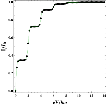
Figure 2: The current-voltage dependencies for small value of coherent state parameter of vibrons, $|z|=0.25$, and for strong electron-vibron interaction $\lambda=1$. The black dotted curve corresponds to numerical calculation of current when the vibrons are in the coherent state. The thin green curve represents $I-V$ characteristics when the vibrons are in equilibrium and characterized by the effective temperature $T^{*}$ determined by Eq.(30). In calculations the values $T/\hbar\omega=0.05,\Gamma/\hbar\omega=0.001$ was used.

It is physically clear that in this case both systems are close to their ground state (the average number of vibrons $\textless n\textgreater\ll 1$) and there is no difference in the behavior of coherent and non-coherent vibrons. The strong differences appear for large amplitudes of oscillations when $|z|\gg 1$ (see Fig.3 where the dotted curve corresponds to vibrons in the coherent state with parameter $|z|=10$). It is useful to introduce effective temperature of vibrons $T^{\ast}$ by equating the average number of vibrons in coherent and equilibrium state,

$$|z|^{2}=(\exp(\hbar\omega/T^{\ast}))-1)^{-1}.$$ (30)

Then for large amplitudes of oscillations ($|z|\gg 1$) and moderately strong electron-vibron interaction ($\lambda\sim 1$) $T^{\ast}\simeq|z|^{2}\hbar\omega\gg\lambda^{2}\hbar\omega$. It is clear that at these high temperatures of the leads Franck-Condon steps in $I-V$ characteristics will be smeared out. It means that coherent vibrons for large amplitudes of QD oscillations lead to strong suppression of current at low biases and to pronounced step-like behavior of $I-V$ curves. It is interesting to compare this behavior with the Franck-Condon theory by assuming that the vibronic subsystem is hot (it is described by Bose-Einstein distribution with the temperature $T^{\ast}$), while the leads are kept at low temperatures $T\ll\hbar\omega$. The thin curve (green on-line) in Fig.3 demonstrates this case.

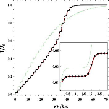
Figure 3: $I-V$ plots for the large value of the parameter $|z|=10$ . All other parameters are the same as in Fig.2. The thin green curve corresponds to the case of equilibrated vibrons with the effective temperature determined by the parameter $|z|=10$. The red dash-dotted curve represents calculation of current in the approximation when $\rho_{0}=0.5$ (see the text bellow). Inset shows the region of low voltages.

We see rather strong differences in current-voltage dependencies: (i) the height of the steps for coherent vibrons are not regular, and (ii) the current in the case of coherent vibrons saturates at lower voltages ($eV_{s}\simeq|z|\hbar\omega$) than for equilibrated vibrons.

One can strongly simplify numerical calculations noticing that coefficient $\rho_{0}$ (zeroth harmonic) of the Fourier series Eq.(22) in the steady state regime $\rho_{0}=0.5$ with very high accuracy, $\sim 10^{-5}$. Then if we put in Eq. (29) $\rho_{0}=1/2$ and $\rho_{p}=0$ for $p\geq 1$, one gets a simple analytic formula for the average current

$$I=I_{0}\sum_{n}a_{n}\left[f_{L}(\varepsilon_{0}-n\omega)-f_{R}(\varepsilon_{0}-n\omega)\right],$$ (31)

where

$$a_{n}=\frac{1}{\pi}\int_{0}^{\pi}d\vartheta\text{e}^{-\lambda^{2}(1-\cos{\vartheta})}\times$$

$$\hskip 28.45274pt\times\cos{n\vartheta}\cos{(\lambda^{2}\sin{\vartheta})}J_{0}\left(4\lambda|z|\sin{\frac{\vartheta}{2}}\right).$$ (32)

For $\lambda\leq 1$ one can roughly estimate integral Eq.(III) as $a_{n}\simeq J_{n}^{2}\left(2\lambda|z|\right)$. This allows us to strongly simplify numerical calculations. Note that Eq.(31) has the same form as a well-known equation (see e.g. Ref.krivepalevskij ) for the current of spinless electrons through a vibrating QD with equilibrated vibrons

$$I_{eq}=I_{0}\sum_{n}A_{n}\left[f_{L}(\varepsilon_{0}-n\omega)-f_{R}(\varepsilon_{0}-n\omega)\right],$$ (33)

where now spectral densities $A_{n}$ are defined by the expression $\text{Tr [e}^{-\imath\lambda p(t)}\text{e}^{\imath\lambda p(0)}\rho_{eq}]=\sum_{n}A_{n}e^{\imath\omega nt}$.

The dash-dotted curve (red on-line) in the Fig.3 correspond to calculations by using Eqs.(31),(III). This approximate calculations coincide with the ”exact” numerical calculations with a high accuracy.

In summary, we have calculated $I-V$ characteristics of a single-molecule transistor, assuming vibrons of QD (molecule) oscillations to be in a coherent state. It was shown that $I-V$ curves at low temperatures have a step-like form similar to the steps that accompany the lifting of Franck-Condon blockade by bias voltage. However, for large amplitudes of oscillations there are strong differences in the predictions of the Franck-Condon theory and our model. By using numerical calculations we found strong suppression of conductance even for a weak or moderately strong electron-vibron coupling. The lifting of this coherent oscillations-induced blockade by a bias voltage occurs at voltages much lower then the ones predicted by the Franck-Condon theory.

Acknowledgements. The authors thank L.Y.Gorelik and O.A.Ilinskaya for useful discussions. This work is supported by the National Academy of Sciences of Ukraine (grant No. 4/19-N and Scientific Program 1.4.10.26.4) and partially by the Institute for Basic Science in Korea.

References

• (1) Y. G. Naidyuk and I. K. Yanson, Point Contact Spectroscopy, Springer Series in Solid-State Sciences 145 (2005)(New York: Springer).
• (2) H.Park, J.Park, A.K.L.Lim, E.H.Anderson, A.P.Alivisatos, P.L.McEuen, Nature 407, 57-60 (2000)
• (3) P. Utko, R. Ferone, I. V. Krive, R.I. Shekhter, M. Jonson, M. Monthioux, L. Noé, J. Nygård, Nature Communications 1, 37 (2010)
• (4) B. Babić, J. Furer, S. Sahoo, Sh. Farhangfar, C. Schönenberger, Nano Letters 3, 11, 1577-1580, (2003)
• (5) R. Leturcq, C. Stampfer, K. Inderbitzin, et al., Nature Phys. 5, 327–331, (2009)
• (6) M.Poot and H.S.J. van der Zant, Phys. Rep. 511, 273, (2012)
• (7) J.Koch and F.von Oppen, Phys.Rev.Lett.94, 206804 (2005)
• (8) J.U.Kim, I.V.Krive, J.M.Kinaret, Phys.Rev.Lett.90, 6401 (2003)
• (9) W. Liu, F. Wang, Z. Tang, R. Liang, Nanomaterials 9, 863, (2019)
• (10) W. Liu, F. Wang, Z. Tang, R. Liang, Nanomaterials 9, 394, (2019)
• (11) A. Mitra, I. Aleiner and A. J. Millis, Phys.Rev.B 69, 245302, (2004)
• (12) J-P. Gazeau, Coherent States in Quantum Physics, Wiley-VCH, Berlin, 2009
• (13) A.Zazunov, D.Feinberg, and T.Martin, Phys.Rev.Lett. 97, 196801, (2006)
• (14) A. Blais, S.M. Girvin and W.D. Oliver, Nat. Phys. 16, 247–256, (2020)
• (15) I.V. Krive, A. Palevski, R.I. Shekhter, and M. Jonson, Low Temperature Physics 36, 119, (2010)
• (16) A.D.Shkop, O.M.Bahrova, S.I.Kulinich, I.V.Krive, Superlattices and Microstructures 137, 106356, (2020)
• (17) N. S. Wingreen, K. W. Jacobsen, and J. W. Wilkins, Phys.Rev.B 40, 11834, (1989)