A bipartite Sachdev-Ye-Kitaev model:
Conformal limit and level statistics

Abstract

We study a bipartite version of the Sachdev-Ye-Kitaev (SYK) model. We show that the model remains solvable in the limit of large-$N$ in the same sense as the original model if the ratio of both flavors is kept finite. The scaling dimensions of the two species can be tuned continuously as a function of the ratio. We also investigate the finite-size spectral properties of the model. We show how the level statistics differs from the original SYK model and infer an additional exchange symmetry in the bipartite model.

I Introduction

The Sachdev-Ye-Kitaev (SYK) model [1, 2, 3, 4, 5] describes a system with many degrees of freedom with random all-to-all ($q$-body) interactions. The original model of Sachdev and Ye consists of pairwise coupled SU($M$) spins [1]. The more recent version proposed by Kitaev [3] has $N_{\chi}\gg 1$ Majorana sites. The $q=4$ version has the Hamiltonian

$$H_{\text{SYK}}=\frac{1}{4!}\sum_{i,j,l,m}J_{ijlm}\gamma_{i}\gamma_{j}\gamma_{l}\gamma_{m}\;.$$ (1)

with $N_{\chi}$ localized Majorana fermions $\gamma_{i}$ with $i=1,...,N_{\chi}$. The term SYK is also used to refer to complex-fermion versions of this model and models with $q$-body interactions, with $q$ taking values other than $4$. In this work, we will restrict to the Majorana version (1) with four-body interactions. The Majorana degrees of freedom have no kinetic energy in this setup; in fact, since the interactions are all-to-all, the system has zero spatial dimensions. The interactions are usually taken to be Gaussian with mean $\langle J_{ijlm}\rangle=0$ and variance

$$\langle J_{ijlm}J_{i^{\prime}j^{\prime}l^{\prime}m^{\prime}}\rangle=\frac{6J^{2}}{N_{\chi}^{3}}\delta_{i,i^{\prime}}\delta_{j,j^{\prime}}\delta_{l,l^{\prime}}\delta_{m,m^{\prime}}.$$

The SYK model has been studied intensely in the last few years, and has a number of fascinating properties. It is a strongly coupled quantum many-body system that is maximally chaotic, as evidenced by a maximal Lyapunov exponent extracted from out-of-time-ordered correlators, and hence acts as a fast scrambler of quantum information [4, 5, 6]. It is nearly conformally invariant, and is exactly solvable in the large $N_{\chi}$ limit [7, 4, 8, 9, 10]. It has been used to describe two dimensional gravity and black holes [2, 3, 4, 11, 12, 9]. The SYK model and its extensions have also been used as a mean field model for non-Fermi liquids, and metals without quasiparticles [13, 14, 15, 16, 17, 18, 19].

The subject of this work is a variant of the SYK model, which we henceforth refer to as the bipartite SYK (b-SYK) model. The b-SYK was reported recently in Ref. [20] by two of the present authors to arise as the effective low-energy model in finite-size strained Kitaev honeycomb systems in the presence of the so-called $\Gamma$-term and moderate disorder. The b-SYK consists of two sets of Majorana fermions, $A$ and $B$, with random 4-body interaction terms that each involve exactly two Majorana fermions from $A$ and two from $B$. The difference with the standard SYK model is that there are no interactions within each set, only between the sets. This is illustrated in a sketch in Fig. 1.

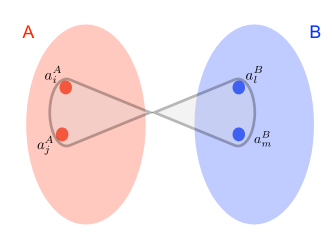
Figure 1: Graphical representation of the b-SYK model. Two sets of Majorana fermions, $A$ and $B$, do not interact within the set but strongly interact between sets.

The b-SYK model Hamiltonian is

$$H_{\text{b-SYK}}=\frac{1}{4}\sum_{i,j=1}^{N_{A}}\sum_{l,m=1}^{N_{B}}J_{ijlm}a_{i}^{A}a_{j}^{A}a_{l}^{B}a_{m}^{B}\;,$$ (2)

where $a^{A}$ is a Majorana fermion in set $A$ whereas $a^{B}$ is one in set $B$. There are $N_{A}$ and $N_{B}$ fermions in the two sets, respectively. The distribution of the couplings follows

$$\langle J_{ijlm}J_{i^{\prime}j^{\prime}l^{\prime}m^{\prime}}\rangle=\frac{J^{2}}{2\sqrt{N_{A}N_{B}}^{3}}\delta_{i,i^{\prime}}\delta_{j,j^{\prime}}\delta_{l,l^{\prime}}\delta_{m,m^{\prime}}\;.$$

We show that the b-SYK model has an asymptotic conformal symmetry in the large-$N_{\chi}$ limit with tunable scaling dimensions — the scaling dimensions are a function of the relative sizes of the $A$ and $B$ sets. By exploring the level statistics in finite-size realizations of the system, we infer that the b-SYK system has an additional ${\mathbb{Z}_{2}}$ symmetry compared to the SYK system when the two sets contain equal numbers of Majorana fermions.

In Sec. II we study the large-$N_{\chi}$ limit of the theory, deriving relations for the two-point correlator and the scaling dimensions. In Sec. III we study the level statistics of the b-SYK Hamiltonian and of the Hamiltonian interpolating between b-SYK and SYK. The findings of the paper and their context are discussed in Sec. IV

II Some analytical properties in the conformal limit

One of the features of the SYK model is that it shows conformal invariance in the infrared in the large-$N_{\chi}$ limit. This allows for an asymptotically exact solution of its correlation functions [4]. We find that the emerging conformal symmetry of the SYK model also carries over to the b-SYK model if the large-$N_{\chi}$ limit is taken in a specific way: the conformal symmetry exists in the limit $N_{A},N_{B}\to\infty$ as long as the ratio $N_{A}/N_{B}=\kappa$ is kept constant. Consequently, instead of having one scaling dimension of the Majorana fermions, like in the SYK model, the two sets of Majorana fermions, $A$ and $B$, generally have different scaling dimensions, $\Delta_{A}$, and $\Delta_{B}$. Their scaling dimensions depend on the parameter $\kappa$, and they can assume values between $0$ and $1/2$ while $\Delta_{A}+\Delta_{B}=1/2$.

To demonstrate this, we first define the imaginary time-ordered correlation functions

$$\begin{split}G^{AA}_{ij}(\tau)=\langle T_{\tau}\left(a^{A}_{i}(\tau)a^{A}_{j}(0)\right)\rangle\;;\\ G^{BB}_{ij}(\tau)=\langle T_{\tau}\left(a^{B}_{i}(\tau)a^{B}_{j}(0)\right)\rangle\;;\\ G^{AB}_{ij}(\tau)=\langle T_{\tau}\left(a^{A}_{i}(\tau)a^{B}_{j}(0)\right)\rangle\;;\\ G^{BA}_{ij}(\tau)=\langle T_{\tau}\left(a^{B}_{i}(\tau)a^{A}_{j}(0)\right)\rangle\;.\end{split}$$ (3)

The Green function of the non-interacting problem is given by

$$\begin{split}G^{AA}_{0,ij}(\tau)&=\frac{1}{2}\rm{sgn}(\tau)\delta_{i,j}\;,\\ G^{BB}_{0,ij}(\tau)&=\frac{1}{2}\rm{sgn}(\tau)\delta_{i,j}\;\\ G^{AB}_{0,ij}(\tau)=G^{BA}_{0,ij}(\tau)&=0\;.\end{split}$$ (4)

meaning it is local in the index $i,j$ as well as the set label $A,B$. It constitutes the starting point for the perturbation theory to follow. The most general Dyson equation reads

$$\int d\tau^{\prime}\left(\begin{array}[]{cc}G^{AA-1}_{0,ij}(\tau,\tau^{\prime})-\Sigma^{AA}_{ij}(\tau,\tau^{\prime})&G^{AB-1}_{0,ij}(\tau,\tau^{\prime})-\Sigma^{AB}_{ij}(\tau,\tau^{\prime})\\ G^{BA-1}_{0,ij}(\tau,\tau^{\prime})-\Sigma^{BA}_{ij}(\tau,\tau^{\prime})&G^{BB-1}_{0,ij}(\tau,\tau^{\prime})-\Sigma^{BB}_{ij}(\tau,\tau^{\prime})\end{array}\right)\left(\begin{array}[]{cc}G^{AA}_{jk}(\tau^{\prime},\tau^{\prime\prime})&G^{AB}_{jk}(\tau^{\prime},\tau^{\prime\prime})\\ G^{BA}_{jk}(\tau^{\prime},\tau^{\prime\prime})&G^{BB}_{jk}(\tau^{\prime},\tau^{\prime\prime})\end{array}\right)=\delta(\tau-\tau^{\prime\prime})\delta_{i,k}\mathds{1}$$ (9)

where $\Sigma^{AA}$, $\Sigma^{AB}$, $\Sigma^{BA}$, and $\Sigma^{BB}$ are the self-energies whereas $G^{AA}$, $G^{AB}$, $G^{BA}$, and $G^{BB}$ are the Green functions. Summation over double indices is implied. In general, this equation is non-local in both the indices $i,j$ as well as the set labels $A,B$. The most transparent way to determine the self-energies is based on a diagrammatic representation of perturbation theory in terms of Feynman diagrams. To leading order in $N_{A}$ and $N_{B}$, the diagrams shown in Fig. 2 constitute the entire perturbative series and can be resummed exactly. This implies that in this limit, the theory remains local in $i,j$ as well as $A,B$. Consequently, to leading order the off-diagonal self-energies $\Sigma^{AB}_{ii}(\tau_{1},\tau_{2})$ as well as the off-diagonal Green functions $G^{AB}$ and $G^{BA}$ vanish. We can drop the subscripts $i,j$, as all $\Sigma$’s and $G$’s are diagonal in these indices and independent of $i$. Furthermore, the self-energies $\Sigma^{AA}_{ii}(\tau_{1},\tau_{2})$ and $\Sigma^{BB}_{ii}(\tau_{1},\tau_{2})$ dominate the bare propagators, Eq. (4), in the infrared.

Thus, the Dyson equation reduces to

$$\int d\tau^{\prime}\left(\begin{array}[]{cc}\Sigma^{AA}(\tau,\tau^{\prime})G^{AA}(\tau^{\prime},\tau^{\prime\prime})&0\\ 0&\Sigma^{BB}(\tau,\tau^{\prime})G^{BB}(\tau^{\prime},\tau^{\prime\prime})\end{array}\right)=-\delta(\tau-\tau^{\prime\prime})\mathds{1}\;.$$ (13)

Utilizing translational invariance in time and passing over to frequency space using a Fourier transformation, we obtain

$$\Sigma^{AA}\left(\omega\right)G^{AA}\left(\omega\right)=-1;\qquad\Sigma^{BB}\left(\omega\right)G^{BB}\left(\omega\right)=-1.$$ (15)

We now consider the leading-order approximation shown in the diagrams of Figure 2:

$$\begin{split}\Sigma^{AA}(\tau)&=\frac{J^{2}N_{A}N_{B}^{2}}{\sqrt{N_{A}^{3}N_{B}^{3}}}G^{AA}(\tau)G^{BB}(\tau)G^{BB}(\tau)=\frac{J^{2}}{\sqrt{\kappa}}G^{AA}(\tau)G^{BB}(\tau)G^{BB}(\tau)\\ \Sigma^{BB}(\tau)&=\frac{J^{2}N_{A}^{2}N_{B}}{\sqrt{N_{A}^{3}N_{B}^{3}}}G^{BB}(\tau)G^{AA}(\tau)G^{AA}(\tau)=J^{2}\sqrt{\kappa}G^{BB}(\tau)G^{AA}(\tau)G^{AA}(\tau)\;.\end{split}$$ (16)

Because of translational invariance in time, all $G$’s and $\Sigma$’s only contain relative coordinates; hence they each have a single time argument instead of two.

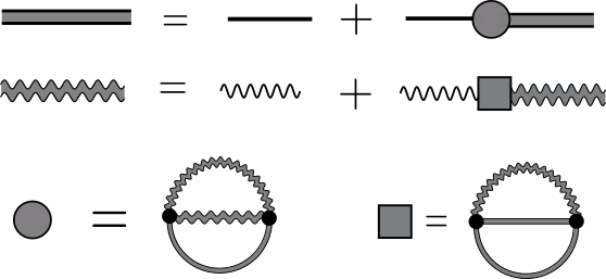
Figure 2: The straight line denotes the propagator $G^{AA}$ whereas the wiggly line is $G^{BB}$. The upper line shows the Dyson equation for $G^{AA}$ and the second line the Dyson equation for $G^{BB}$, compare Eq. (13). The lowest line shows the approximation for the self-energies $\Sigma^{AA}$ and $\Sigma^{BB}$, Eq. (16), which becomes exact in the limit of large $N_{A}$ and $N_{B}$.

Due to the time reparametrization symmetry of the theory we expect conformal invariance. Since we are expecting different scaling dimensions for the Majorana fermions in the two sets we introduce the scaling dimension $\Delta_{A}$ for Majorana fermions in set $A$, whereas we introduce $\Delta_{B}$ for those in set $B$. We then have

$$\begin{split}G^{AA}(\tau)&=C_{A}\frac{\rm{sgn}(\tau)}{|\tau|^{2\Delta_{A}}},\\ G^{BB}(\tau)&=C_{B}\frac{\rm{sgn}(\tau)}{|\tau|^{2\Delta_{B}}},\end{split}$$ (17)

for the full Green functions. Here $C_{A}$ and $C_{B}$ are constants. Inserting this conformal anzatz into Eqs. (16), the self energies read

$$\begin{split}\Sigma^{AA}\left(\tau\right)&=\frac{1}{\sqrt{\kappa}}J^{2}C_{A}C_{B}^{2}\frac{\rm{sgn}\left(\tau\right)}{\left|\tau\right|^{2\Delta_{A}+4\Delta_{B}}},\\ \Sigma^{BB}\left(\tau\right)&=\sqrt{\kappa}J^{2}C_{B}C_{A}^{2}\frac{\rm{sgn}\left(\tau\right)}{\left|\tau\right|^{2\Delta_{B}+4\Delta_{A}}},\end{split}$$ (18)

where $\kappa=N_{A}/N_{B}$.

We now express Eqs. (17) and (18) in frequency space. Using the identity

$$\int_{-\infty}^{\infty}d\tau e^{\imath\omega\tau}\frac{\rm{sgn}(\tau)}{|\tau|^{\alpha}}=\imath\sqrt{\pi}\frac{\Gamma\left(1-\frac{\alpha}{2}\right)}{\Gamma\left(\frac{1}{2}+\frac{\alpha}{2}\right)}\rm{sgn}(\omega)\left(\frac{\left|\omega\right|}{2}\right)^{\alpha-1},$$ (19)

we obtain for the Green functions

$$G^{AA}\left(\omega\right)=C_{A}\imath\sqrt{\pi}\frac{\Gamma\left(1-\Delta_{A}\right)}{\Gamma\left(\frac{1}{2}+\Delta_{A}\right)}\rm{sgn}\left(\omega\right)\left(\frac{\left|\omega\right|}{2}\right)^{2\Delta_{A}-1},$$

and similarly for $G^{BB}\left(\omega\right)$. Applying the Fourier transform to Eqs. (18) and using the same identity, we obtain for the self energies

$$\Sigma^{AA}\left(\omega\right)= \frac{J^{2}}{\sqrt{\kappa}}C_{A}C_{B}^{2}\imath\sqrt{\pi}\frac{\Gamma\left(1-\Delta_{A}-2\Delta_{B}\right)}{\Gamma\left(\frac{1}{2}+\Delta_{A}+2\Delta_{B}\right)}$$

$$\quad\times\rm{sgn}\left(\omega\right)\left(\frac{\left|\omega\right|}{2}\right)^{2\Delta_{A}+4\Delta_{B}-1},$$

and similarly for $\Sigma^{BB}$ with $\kappa\to 1/\kappa$.

We can now use these expressions in our frequency-space Dyson equation, Eq. (15). The first equation (for $A$) then reads

$$-1= -\frac{J^{2}}{\sqrt{\kappa}}C_{A}^{2}C_{B}^{2}\pi\left(\frac{\left|\omega\right|}{2}\right)^{4\Delta_{A}+4\Delta_{B}-2}$$

$$\quad\times\frac{\Gamma\left(1-\Delta_{A}-2\Delta_{B}\right)}{\Gamma\left(\frac{1}{2}+\Delta_{A}+2\Delta_{B}\right)}\frac{\Gamma\left(1-\Delta_{A}\right)}{\Gamma\left(\frac{1}{2}+\Delta_{A}\right)}.$$

Since the left-hand side is $\omega$-independent, we need to remove the $\omega$ dependence on the right-hand side. Imposing the condition leads to the result

$$\Delta_{A}+\Delta_{B}=\frac{1}{2}$$ (20)

as announced at the beginning of this section.

Defining $\Lambda=\pi J^{2}C_{A}^{2}C_{B}^{2}$, the Dyson equations now read

$$\begin{split}1=&\frac{\Lambda}{\sqrt{\kappa}}\frac{\Gamma\left(1-\Delta_{A}-2\Delta_{B}\right)}{\Gamma\left(\frac{1}{2}+\Delta_{A}+2\Delta_{B}\right)}\frac{\Gamma\left(1-\Delta_{A}\right)}{\Gamma\left(\frac{1}{2}+\Delta_{A}\right)},\\ 1=&\sqrt{\kappa}\Lambda\frac{\Gamma\left(1-2\Delta_{A}-\Delta_{B}\right)}{\Gamma\left(\frac{1}{2}+2\Delta_{A}+\Delta_{B}\right)}\frac{\Gamma\left(1-\Delta_{B}\right)}{\Gamma\left(\frac{1}{2}+\Delta_{B}\right)}.\end{split}$$ (21)

By eliminating $\Lambda$ and using properties of the Gamma function (Appendix A), we can relate $\kappa$ to the scaling dimensions ($\Delta_{A}=\frac{1}{2}-\Delta_{B}$):

$$\kappa=\frac{2\Delta_{A}}{1-2\Delta_{A}}\left(\frac{1}{\tan\left(\pi\Delta_{A}\right)}\right)^{2}\;.$$ (22)

This equation implicitly provides the scaling dimension $\Delta_{A}$ (and hence also $\Delta_{B}$) as a function of the ratio of sizes of the two partitions, $\kappa=N_{A}/N_{B}$. For $\kappa=1$, we find $\Delta_{A}=\Delta_{B}=1/4$, as expected, just like in the standard SYK model. For other values of $\kappa$, both scaling dimensions interpolate between $0$ and $1/2$ while always fulfilling $\Delta_{A}+\Delta_{B}=1/2$. This behavior is presented in Fig. 3 on a logarithmic scale which shows the $A$-$B$ symmetry explicitly. Tunable scaling dimensions have also been seen in other variants of the SYK model e.g. Ref. [21, 22].

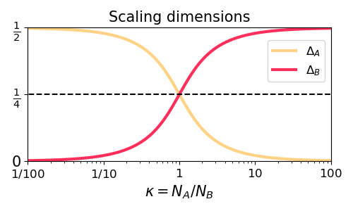
Figure 3: Scaling dimensions $\Delta_{A}$ and $\Delta_{B}$ as a function of $\kappa$. Both interpolate between $0$ and $1/2$.

Due to the conformal invariance and the reparametrization invariance it is straightforward to determine the finite temperature and real time correlators. At finite temperatures we find

$$G^{AA}(\tau) = A\;\rm{sgn}(\tau)\left(\frac{\pi}{\beta\sinh\left(\frac{\pi\tau}{\beta}\right)}\right)^{2\Delta_{A}}\;,$$

$$G^{BB}(\tau) = B\;\rm{sgn}(\tau)\left(\frac{\pi}{\beta\sinh\left(\frac{\pi\tau}{\beta}\right)}\right)^{2\Delta_{B}}\;,$$ (23)

whereas for the retarded propagator at finite temperature we obtain

$$G^{AA}_{\rm{ret}}(t) = \theta(t)A\cos\left(\pi\Delta_{A}\right)\left(\frac{\pi}{\beta\sinh\left(\frac{\pi t}{\beta}\right)}\right)^{2\Delta_{A}}\;,$$

$$G^{BB}_{\rm{ret}}(t) = \theta(t)B\cos\left(\pi\Delta_{B}\right)\left(\frac{\pi}{\beta\sinh\left(\frac{\pi t}{\beta}\right)}\right)^{2\Delta_{B}}\;.$$

III Level statistics

In this section, we focus on the level spacing statistics of the b-SYK model. For this purpose, we consider finite $N_{A}$ and $N_{B}$, and diagonalize the many-body SYK and b-SYK Hamiltonians.

Level statistics can help identify the existence of chaos (non-integrability) in quantum Hamiltonians, and also to distinguish between different symmetry classes. The interest in the SYK model is partly due to its being maximally chaotic. Therefore, eigenvalue statistics has been a widely used diagnostic for characterizing the SYK model [23, 24, 25, 12, 26, 27] and its various variants [28, 29, 30, 31, 32, 26, 33, 34, 35, 36, 37, 38, 39, 40, 41, 42, 43, 44]. A noteworthy feature of the SYK level statistics is that it depends on the number of Majorana fermions $N_{\chi}$. We show below that the level statistics of the b-SYK model in the $N_{A}=N_{B}$ case is systematically shifted with respect to that of the standard SYK model, consistent with the presence of an extra ${\mathbb{Z}_{2}}$ symmetry in the b-SYK system.

III.1 Relevant ensembles

The universality classes of random matrices that are relevant for us include the Gaussian Orthogonal Ensemble (GOE), the Gaussian Unitary Ensemble (GUE), and the Gaussian Symplectic Ensemble (GSE). In Table 1 we refer to these as O, U, and S respectively for conciseness. Additionally, we will encounter below the level statistics obtained by merging the spectra of two GOE matrices; we refer to this as $2\times$GOE, or for conciseness 2O in Table 1.

$N_{\chi}$ (mod 8)	0	1	2	3	4	5	6	7
$H_{\text{SYK}}$	O	O	U	S	S	S	U	O
$H_{\text{b-SYK}}$	2O	2O	O	U	U	U	O	2O

Table 1: Level statistics of the Majorana fermion SYK model, $H_{\text{SYK}}$ as compared to $H_{\text{b-SYK}}$ in (2). Here O=GOE, U=GUE, S=GSE and 2O = 2$\times$GOE are the different universal random matrix ensembles. Note how the level statistics of $H_{\text{b-SYK}}$ traces those of $H_{\text{SYK}}$ but with a reduction in the symmetry classifications of one step such that S $\to$ U $\to$ O $\to$ 2O.

For characterizing the level statistics with a single number, it has become common to use the average ratio of successive level spacings [45, 46]. One starts with calculating the finite size spectrum $E_{n}$, which are ordered from lowest to highest energy. The set of level spacings are defined as $s_{n}=E_{n+1}-E_{n}$. This allows to define the ratio

$$r_{n}=\frac{{\rm min}(s_{n},s_{n-1})}{{\rm max}(s_{n},s_{n-1})}\;.$$ (25)

Analyzing the statistics of this quantity $r_{n}$ has advantages over the statistics of the bare level spacings $s_{n}$ themselves. It bypasses the need to account for a varying density of states through unfolding procedures. In addition, the average of this quantity has characteristic values for the different ensembles, thus enabling one to distinguish symmetry classes without analyzing complete distributions.

For the Wigner-Dyson ensembles, the probability distributions of the ratio $r$ are well-approximated by the surmise [46] $P(r)\propto(r+r^{2})^{\beta}/(1+r+r^{2})^{1+3\beta/2}$ up to normalization, with $\beta=1$ for GOE, $\beta=2$ for GUE, and $\beta=4$ for GSE. The averages of these distributions are found to be $\langle r\rangle_{\rm GOE}\approx 0.53$, $\langle r\rangle_{\rm GUE}\approx 0.60$, and $\langle r\rangle_{\rm GSE}\approx 0.67$ [46].

Integrable (non-chaotic) Hamiltonians, which do not show level repulsion, generically have Poisson statistics, for which the level spacing ratio has probability distribution $P(r)=2/(1+r)^{2}$ and mean value $\langle r\rangle=2\ln 2-1\approx 0.39$. An integrable system can be thought of as having a large number of conserved quantities or quantum numbers. Therefore, adding one or a few conservation laws to a GOE system is expected to change the distribution to a form intermediate between the GOE and Poisson cases. The $2\times$GOE spectrum can be interpreted as that obtained when a GOE system acquires a single quantum number with two possible values, which splits the GOE spectrum into two sectors. Thus, we expect its level spacing distribution to be intermediate between Poisson and GOE distributions. Indeed, we find numerically, by merging the spectra of two GOE matrices, that the $2\times$GOE distribution has $\langle{r}\rangle\approx 0.425$, intermediate between the Poisson and GOE values. Some analytic formulas for the $2\times$GOE distribution were also provided in Refs. 47, 48.

As discrete symmetries are common in quantum Hamiltonians, spectra formed out of two or more independent GOE or GUE components are the subject of longstanding interest in the quantum-chaos and random-matrix literature [49, 50, 51, 52, 53, 54, 55, 56, 57, 58, 59, 35, 60, 47, 48]. Here, we will only be concerned with the $2\times$GOE case because restricting the couplings of the SYK Hamiltonian to obtain the b-SYK Hamiltonian effectively adds a single ${\mathbb{Z}_{2}}$ symmetry.

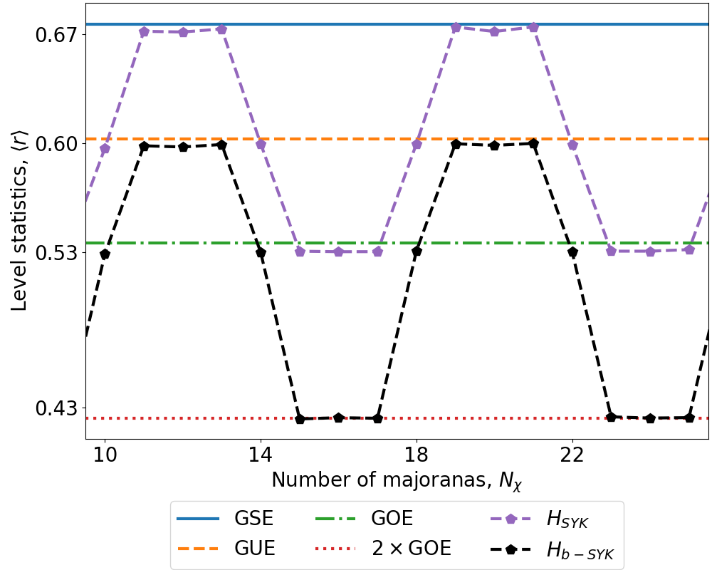
Figure 4: Average level spacing ratio $\langle r\rangle$ for $H_{\text{SYK}}$ and $H_{\text{b-SYK}}$, plotted against system size $N_{\chi}$. For each system size, the value of $\langle r\rangle$ for $H_{\text{b-SYK}}$ is lower than that for $H_{\text{SYK}}$. The SYK-model has an 8-fold periodicity [24, 25, 12, 26] related to the Bott periodicity. The overall $\langle r\rangle$ vs $N_{\chi}$ behavior for $H_{\text{b-SYK}}$ mimics that for $H_{\text{SYK}}$ but with a shifted classification. Thus instead of the SYK sequence we get a relative shift as O$\to$2O, U$\to$O and S$\to$U.

III.2 Level statistics of b-SYK

In the case of the SYK model, the random matrix ensemble describing the level statistics changes with the number of Majorana fermions $N_{\chi}$ [24, 25, 12, 26] as listed in Table 1. This dependence is cyclic modulo $8$ in $N_{\chi}$ and is related to the 8-fold Bott-periodicity. Here we will compare the level spacing statistics properties of the SYK model to that of the b-SYK model. We will concentrate on the case $\kappa=1$, and we choose $N_{\chi}=2N_{a}=2N_{b}$ or $N_{\chi}=2N_{a}+1=2N_{b}-1$ depending on the parity of $N_{\chi}$.

The numerical procedure used to obtain level statistics is described briefly in Appendix B.

We quantify the level statistics by the average ratio $\langle{r}\rangle$, described above. Some results are summarized in Fig. 4, for both the SYK and the b-SYK Hamiltonians. For each $N_{\chi}$, the averaging of the spacing ratio is performed over the spectra of many coupling realizations so that the results are sufficiently converged. In Fig. 4 the horizontal lines represent the average $r$ values for different relevant ensembles, as discussed above.

We observe that the average spacing ratio of the b-SYK model is always lower than the average spacing ratio expected from the SYK model, irrespective of the size of the system. However, it follows the same 8-fold periodicity in the total number of Majorana fermions, $N_{\chi}$. Compared to the SYK sequence, we find relative shifts O$\to$2O, U$\to$O, S$\to$U, i.e., the GSE, GUE, and GOE get converted to GUE, GOE, and $2\times$GOE respectively. The shift is also seen by comparing the two rows of Table 1.

Going beyond the average, in Figure 5 we show the full distributions (numerical histograms) of the level spacing ratio, for the $H_{\text{b-SYK}}$ Hamiltonian with $N_{\chi}=21,25,26$. Clearly, the three classes follow the expected distributions for $2\times$GOE, GOE, and GUE, shown as dotted lines. The GSE distribution is not obtained in the b-SYK system for any value of $N_{\chi}$.

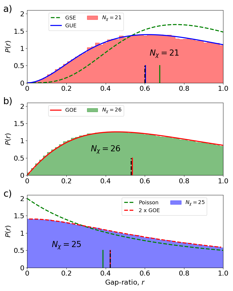
Figure 5: Distribution of level spacing ratios for the b-SYK Hamiltonian with $N_{\chi}=21,25,26$, corresponding to the three distinct classes listed in Table 1. The distributions for a) $N_{\chi}=21$ and b) $N_{\chi}=26$ match well the expected surmise for the GUE and GOE classes. The third example, c) $N_{\chi}=25$, closely follows the 2$\times$GOE distribution. The GSE and Poissonian distributions are also shown as lines. None of the b-SYK distributions follow the GSE class (in contrast to the SYK case) or the Poissonian distribution. The vertical lines are a visual representation of the mean $\left<r\right>$ for the various distributions.

The shift in level statistics relative to SYK is clearly due to the restriction to bipartite interactions. The results are consistent with the explanation that the bipartite structure leads to an additional ${\mathbb{Z}_{2}}$ symmetry of the Hamiltonian. A system of the GUE symmetry class, if endowed with an additional ${\mathbb{Z}_{2}}$ symmetry, shows GOE level statistics [61, 62, 63, 64]. This effect was discussed early in the context of single-particle (billiard) systems with a magnetic field [61, 62]. This system would naively be expected to have GUE statistics due to broken time-reversal symmetry. However, when reflection symmetry is present, the level statistics is of the GOE class. This phenomenon has also been observed in a many-body system [65]. In the present case, the anti-unitary symmetry involved is not time, but the effect is the same: For $N_{\chi}=10,14,18,22\ldots$, the SYK level statistics are GUE, but the b-SYK level statistics are of GOE type.

For values of $N_{\chi}$ for which the level statistics if of GSE type, a corresponding effect is seen. The additional symmetry reduces the degree of level repulsion, and one obtains GUE statistics instead, as seen in Fig. 4 and Table 1. A GSE to GUE shift due to a parity symmetry is discussed in Section 2.7 of Ref. [58]. Still, we do not know of another example in the literature involving a many-body Hamiltonian. The b-SYK spectrum retains the Kramers degeneracy; the level repulsion is between pairs of degenerate states.

III.3 The ${\mathbb{Z}_{2}}$ symmetry

The numerical data implies that the b-SYK Hamiltonian possesses a ${\mathbb{Z}_{2}}$ symmetry which is not present in the SYK model.

The extra symmetry arises because the b-SYK restriction removes terms in the Hamiltonian that has an odd number of $A$ fermions, or an odd number of $B$ fermions. Each b-SYK term has exactly two $A$ fermions and exactly two $B$ fermions. Because each term is bilinear in the $a_{j}^{A}$’s as well as in the $a_{j}^{B}$’s, if one flips the signs of all the $A$ operators, while keeping all the $B$ operators fixed, each term in the Hamiltonian would remain unchanged.

Thus, the b-SYK model admits a global sign flip symmetry $a_{j}^{A}\to-a_{j}^{A}$, $a_{j}^{B}\to+a_{j}^{B}$. In contrast to the b-SYK model, the SYK model is not invariant under this transformation, as the usual SYK model also contains terms of the form $a_{i}^{A}a_{j}^{B}a_{k}^{B}a_{l}^{B}$ and $a_{i}^{A}a_{j}^{A}a_{k}^{A}a_{l}^{B}$. Since these terms have an odd number of both $a^{A}$ and $a^{B}$ Majoranas, they would change sign under a sign change of only $a^{A}$’s (or a sign change of only $a^{B}$’s).

For even $N_{A}$, the sign flip operation can be expressed in terms of the Hermitian operator

$$\Gamma=\imath^{N_{A}/2}\prod_{i=1}^{N_{A}}a^{A}_{i}.$$ (26)

Using Majorana anticommutation relations, one finds that this operator satisfies $\Gamma a^{A}_{j}=-a^{A}_{j}\Gamma$, provided that $N_{A}$ is even. For odd $N_{A}$, an additional fictitious Majorana has to be added to the product to construct a Hermitian sign-flip operator.

Equivalently, one could flip the signs of the $B$ Majorana operators, and keep the b-SYK Hamiltonian invariant. This is not an independent extra symmetry compared to the SYK model, as the flipping of all Majoranas leaves even the SYK Hamiltonian invariant. Thus, the b-SYK Hamiltonian has a single extra ${\mathbb{Z}_{2}}$ symmetry compared to the SYK Hamiltonian. This explains our observation of a systematic shift of level statistics, described in the previous subsection.

The operator $\Gamma$ can also be regarded as a particle-hole conjugation operator. If each $A$ Majorana is paired with a $B$ Majorana so that the Hilbert space is expressed in terms of complex (usual) fermion Fock space, as described in Appendix B, then flipping signs of $a^{A}_{j}$’s amounts to a transmutation of creation operators of complex fermions into annihilation operators and vice versa, i.e., a particle-hole conjugation. (In terms of the original Majoranas, the $\Gamma$ operator changes a $n$-Majorana state $a^{A}_{1}a^{A}_{2}\ldots a^{A}_{n}\left|0\right\rangle$ to a $(N_{A}-n)$-Majorana state $a^{A}_{n+1}a^{A}_{n+2}\ldots a^{A}_{N_{A}}\left|0\right\rangle$.) Thus, the ${\mathbb{Z}_{2}}$ symmetry can be regarded as a particle-hole conjugation symmetry, if we use the representation that each $A$ Majorana is paired with a $B$ Majorana.

We note parenthetically that the b-SYK Hamiltonian also admits a number of operations that leave the Hamiltonian isospectral, although not invariant: Exchanging any one of the $A$-fermions with any one of the $B$-fermions leaves the Hamiltonian isospectral, i.e., amounts to unitary operations. This emerges due to the restriction from SYK to b-SYK: For the SYK Hamiltonian, such operations are not isospectral. For both SYK and b-SYK, bi-partitioning the Majorana fermions into arbitrary halves and then exchanging the two halves is an isospectral (unitary) operation. The extra feature of the b-SYK is that exchanging a single $A$ fermion with a single $B$ fermion is also a unitary operation.

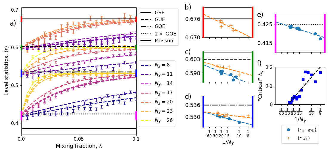
Figure 6: Level statistics when tuning between $H_{\text{b-SYK}}$ and $H_{\text{SYK}}$ Hamiltonians, with $\lambda=0$ ($\lambda=1$) corresponding to b-SYK (SYK). In panel a) the average spacing ratio $\langle{r}\rangle$ is plotted as a function of $\lambda$. The crossover from $\langle r_{\text{b-SYK}}\rangle$ to $\langle r_{\text{SYK}}\rangle$ is steeper for a larger number of Majoranas $N_{\chi}$. Panels b) - e) zoom in on the regions around the various values of $\langle r_{\text{b-SYK}}\rangle$ and $\langle r_{\text{SYK}}\rangle$ that are obtained. The colors on the vertical axes should help to match with the corresponding regions in panel a). These plots b) - e) show that the large-size limits are consistent with the GSE, GUE, GOE, and $2\times$GOE classes. In panel a) a fit is performed to the function $\langle r_{\text{SYK}}\rangle+(\langle r_{\text{b-SYK}}\rangle-\langle r_{\text{SYK}}\rangle)e^{-\frac{\lambda}{\lambda_{C}}}$ and on panel f) the transition parameter $\lambda_{C}$ is shown. The “critical” $\lambda_{C}$ decreases with increasing $N_{\chi}$.

III.4 Interpolation between $H_{\text{b-SYK}}$ to $H_{\text{SYK}}$

Since the level statistics classification is systematically shifted from $H_{\text{SYK}}$ to $H_{\text{b-SYK}}$ this begs the question what one obtains for a mixture of the two Hamiltonians. We therefore define an interpolation Hamiltonian

$$H_{\text{Mix}}=\left(1-\lambda\right)H_{\text{b-SYK}}+\lambda H_{\text{SYK}}$$

and investigate its level statistics as a function of $\lambda$. In the following analysis, we choose the coupling constants $J$ in (1) and (2) such that the variance of $J_{ijlm}$ in both cases is unity for all system sizes. The main results are summarized in Fig. 6. In panel a) we demonstrate how for already a small SYK-mixing, $\lambda\leq 0.1$, results in a drift of the level statistics from the $H_{\text{b-SYK}}$ to the $H_{\text{SYK}}$ random matrix class. This makes sense because, as soon as interactions are allowed which violate the bipartite restriction, the additional symmetry of the b-SYK Hamiltonian is lost. The crossover happens faster (at even smaller values of $\lambda$) for larger system sizes, indicating that, in the large-$N_{\chi}$ limit, an infinitesimal influence of $H_{\text{SYK}}$ is enough to move the system into the lower-symmetry class of the un-restricted SYK Hamiltonian.

To quantify this size dependence of the $H_{\text{b-SYK}}\to H_{\text{SYK}}$ crossover, we fit $\langle r\rangle$ to the function

$$f(\lambda)=\langle r_{\text{SYK}}\rangle+(\langle r_{\text{b-SYK}}\rangle-\langle r_{\text{SYK}}\rangle)e^{-\frac{\lambda}{\lambda_{C}}}$$

such that $f(0)=\langle r_{\text{b-SYK}}\rangle$, and $f(\lambda\gg\lambda_{C})\to\langle r_{\text{SYK}}\rangle$. $\lambda_{C}$ is the value for which $f(\lambda_{C})=\langle r_{\text{SYK}}\rangle$ to first order, i.e. $f(0)+\lambda_{C}f^{\prime}(0)=\langle r_{\text{SYK}}\rangle$. This function captures the transition from $\langle r_{\text{b-SYK}}\rangle$ to $\langle r_{\text{SYK}}\rangle$ as a function of $\lambda$. The best fit is shown in dashed lines, and the numerical $\langle r\rangle$ is shown with statistical errors.

The shift from $\langle r_{\text{b-SYK}}\rangle$ to $\langle r_{\text{SYK}}\rangle$ takes place at smaller values of $\lambda$ if more Majorana fermions, $N_{\chi}$, are involved (brighter colors). In panel f), this is further illustrated: we plot $\lambda_{C}$ as a function of inverse system size $1/N_{\chi}$. Clearly, $\lambda_{C}$ tends to zero in the large $N_{\chi}$ limit, quantifying the intuition that the shift of behavior happens at smaller $\lambda$ for larger sizes.

In panels b)-e) we show a scaling analysis for $\langle r_{\text{b-SYK}}\rangle$ and $\langle r_{\text{SYK}}\rangle$, using the values at $\lambda=0$ and $\lambda=1$. For $\langle r_{\text{SYK}}\rangle$ (orange plus symbols), the large-size limit is consistent with the known symmetry classes, GOE, GUE, or GSE, based on the value of $N_{\chi}$ mod 8 [24, 25, 12, 26]. For $\langle r_{\text{b-SYK}}\rangle$ (blue circles), the large-size limit is consistent with the values corresponding to $2\times$GOE, GOE, or GUE. In panel b), focusing on the GSE value $\langle{r}\rangle\approx 0.67$, only $\lambda=1$ data (values of $\langle r_{\text{SYK}}\rangle$) are visible. Similarly, in panel e), focusing on the $2\times$GOE value $\langle{r}\rangle\approx 0.425$, only $\lambda=0$ data (values of $\langle r_{\text{b-SYK}}\rangle$) are visible.

IV Discussion & Context

This paper has studied a bipartite version of the quartic ($q=4$) SYK model, which we call b-SYK. It consists of two flavors of Majorana fermions that interact between the sets, but not within — each quartic interaction term involves two Majorana fermions from one set and two from the other set. The model was motivated in Ref. [20] as being realizable in a specific setup of a strained version of the Kitaev honeycomb model.

Variants of the SYK model with two species of fermions have appeared previously, perhaps most prominently with the motivation of modeling eternal traversable wormholes using two quartic SYK models with only quadratic interactions between them [28, 66, 33, 67, 68, 69, 70, 71, 72, 73, 74]. In Ref. [22] the coupling between the two SYK clusters is quartic like ours. Since our b-SYK model has no internal coupling within the two sets, it may be regarded as an infinite-coupling limit of the model of Ref. [22], i.e., the limit in which the intra-set couplings can be neglected. Ref. [75] treats a complex-fermion version. Ref. [76] also considers two SYK clusters and quartic couplings between them, but the sizes of the two clusters are parametrically different, so that one acts as a bath for the other. Several other two-flavor or two-species SYK variants have also appeared in the literature [77, 78, 79, 80].

We study the b-SYK model both analytically and numerically. We find that in the large-$N$ limit, the model remains asymptotically solvable, showing conformal invariance in the infrared. We establish that if we keep the ratio between the flavors a variable, we can continuously tune the scaling dimension of the respective species between $0$ and $1/2$.

For finite system sizes, we analyze the level statistics of the model numerically for $\kappa=1$ ($N_{A}=N_{B}$ or $N_{A}=N_{B}\pm 1$) and compare it to the known level statistics of the SYK model. We find that the level statistics deviates systematically, consistent with the b-SYK model possessing an additional ${\mathbb{Z}_{2}}$ symmetry. The GOE, GUE, and GSE level statistics of the SYK model are reduced to $2\times$GOE, GOE, and GUE classes.

Studying the interpolation between the two models, we find that, for finite sizes, the statistics evolve smoothly from the b-SYK to the SYK as a function of interpolating parameter $\lambda$.

In the quantum chaos literature and in random matrix theory, the GOE-GUE crossover has been studied repeatedly in various contexts [81, 82, 83, 84, 85, 54, 86, 58, 87, 88, 89, 90, 91]. In the present case, we have a GUE to GSE crossover, a GOE to GUE crossover, and a $2\times$GOE to GOE crossover, all in the same Hamiltonian, depending on the number of Majorana fermions, according to the Bott periodicity [24, 25, 12, 26]. In addition, unlike typical models studied in traditional quantum chaos or random matrix theory, we have a well-defined thermodynamic (large $N_{\chi}$) limit. It turns out that, in this limit, the crossover happens extremely rapidly, i.e., the b-SYK statistics is lost already for an infinitesimal mixture of SYK.

The present work opens up a number of new questions. Thermodynamic and thermalization properties, as well as higher-order correlation functions, and Lyapunov exponents, remain to be studied. It may be interesting to see how b-SYK physics is explicitly obtained in the large-interaction limit of the model of Ref. [22], and to investigate the behavior of its complex-fermion version. In addition, the level statistics for unequal-sized bipartitions ($\kappa\neq 1$) also deserves exploration.

Appendix A The scaling dimensions

In this Appendix, we show how equations (21) can be used to derive the relationship, Eq. (22), between the ratio $\kappa=N_{A}/N_{B}$ and (one of) the scaling dimensions.

Dividing one of equations (21) by the other gets rid of $\Lambda$. We also use $\Delta_{B}=\frac{1}{2}-\Delta_{A}$, to obtain

$$\kappa=\frac{\Gamma\left(\Delta_{A}\right)\Gamma\left(1+\Delta_{A}\right)}{\Gamma\left(\frac{1}{2}-\Delta_{A}\right)\Gamma\left(\frac{3}{2}-\Delta_{A}\right)}\frac{\Gamma^{2}\left(1-\Delta_{A}\right)}{\Gamma^{2}\left(\frac{1}{2}+\Delta_{A}\right)}.$$ (27)

Using Euler’s reflection formula

$$\Gamma\left(1-z\right)\Gamma\left(z\right)=\frac{\pi}{\sin\left(\pi z\right)},$$ (28)

we find that

$$\Gamma\left(1-\Delta_{A}\right)\Gamma\left(\Delta_{A}\right) =\frac{\pi}{\sin\left(\pi\Delta_{A}\right)},$$ (29)

$$\Gamma\left(\frac{1}{2}-\Delta_{A}\right)\Gamma\left(\frac{1}{2}+\Delta_{A}\right) =\frac{\pi}{\cos\left(\pi\Delta_{A}\right)}.$$ (30)

These can be used for pairs of products of Gamma functions in Eq. (27), yielding

$$\kappa=\frac{\Gamma\left(1+\Delta_{A}\right)}{\Gamma\left(\frac{3}{2}-\Delta_{A}\right)}\frac{\Gamma\left(1-\Delta_{A}\right)}{\Gamma\left(\frac{1}{2}+\Delta_{A}\right)}\frac{\cos\left(\pi\Delta_{A}\right)}{\sin\left(\pi\Delta_{A}\right)}.$$ (31)

There remains pairs of Gamma functions in the denominator and numerator, which we now proceed to eliminate. By making use of the recursive property $\Gamma\left(1+z\right)=z\Gamma\left(z\right)$ we can write

$$\Gamma\left(1+\Delta_{A}\right) =\Delta_{A}\Gamma\left(\Delta_{A}\right),$$

$$\Gamma\left(\frac{3}{2}-\Delta_{A}\right) =\left(\frac{1}{2}-\Delta_{A}\right)\Gamma\left(\frac{1}{2}-\Delta_{A}\right).$$

Applying these relations, and then again applying (30) and (29), leads to

$$\kappa=\frac{2\Delta_{A}}{1-2\Delta_{A}}\frac{1}{\tan^{2}\left(\pi\Delta_{A}\right)},$$

which is the desired result, Eq. 22.

Appendix B Numerical Calculations

In this Appendix we briefly describe the numerical procedure for obtaining the b-SYK (and SYK) spectra, and make some technical remarks.

To form the basis for the Hilbert space, the $N_{\chi}$ Majorana fermions are paired into complex or ‘usual’ fermions (without spin). For even $N_{\chi}$, this leads to $N_{\chi}/2$ complex fermions, and hence the Hilbert space dimension is $2^{N_{\chi}/2}$. This is a manifestation of Majorana’s representing half a fermionic degree of freedom.

Because the Hamiltonian is quartic, either in terms of the Majorana’s or in terms of the complex fermions, the odd-fermion states and the even-fermion states fall into two disconnected sectors, which may be diagonalized separately and have the same statistics.

One could explicitly introduce complex fermions. For the SYK Hamiltonian (1), we could pair the Majorana fermions as, e.g.,

$$\begin{split}c_{j}^{\dagger}=\frac{1}{2}\left(\gamma_{j}+\imath\gamma_{N_{\chi}-j+1}\right);\\ c_{j}=\frac{1}{2}\left(\gamma_{j}-\imath\gamma_{N_{\chi}-j+1}\right).\end{split}$$ (32)

One can then construct a basis for the Hamiltonian as the Fock basis of these complex fermions, including the vacuum, the one-particle states, the two-particle states, etc.:

$$\begin{split}\left|0\right\rangle,\\ c_{1}^{\dagger}\left|0\right\rangle,c_{2}^{\dagger}\left|0\right\rangle,\ldots,\\ c_{1}^{\dagger}c_{2}^{\dagger}\left|0\right\rangle,c_{1}^{\dagger}c_{3}^{\dagger}\left|0\right\rangle,\ldots,\\ \vdots\\ c_{1}^{\dagger}c_{2}^{\dagger}\ldots c_{N_{\chi}/2}^{\dagger}\left|0\right\rangle.\end{split}$$ (33)

The Hamiltonian (with a particular realization of the random couplings $J_{ijlm}$) can then be represented as a matrix in this basis. It is efficient to construct the matrices separately for the even-occupancy and odd-occupancy sectors, since they are decoupled. Either or both of these $2^{N_{\chi}/2-1}\times 2^{N_{\chi}/2-1}$ matrices can then be numerically diagonalized to obtain the spectrum. To obtain sufficient statistics, this procedure is repeated for many different realizations of the random couplings, and the data for level spacings (or level spacing ratios) are aggregated.

In practice, it is not necessary to explicitly express the Hamiltonian in terms of complex fermions. Combining $\gamma_{j}$ and $\gamma_{N_{\chi}-j+1}$ into a complex fermion mode is equivalent to insisting that the vacuum has the property that $\gamma_{j}\left|0\right\rangle$ and $\imath\gamma_{N_{\chi}-j+1}\left|0\right\rangle$ are the same state, for each $j=1,2,\ldots,\frac{N_{\chi}}{2}$. Thus, one can express the basis states as

$$\left|0\right\rangle,\;\gamma_{1}\left|0\right\rangle,\gamma_{2}\left|0\right\rangle,\ldots,\;\gamma_{1}\gamma_{2}\left|0\right\rangle,\gamma_{1}\gamma_{3}\left|0\right\rangle,\ldots,\\ \ldots,\quad\gamma_{1}\gamma_{2}\ldots\gamma_{N_{\chi}/2}\left|0\right\rangle.$$ (34)

and the Hamiltonian matrix elements is calculated directly in this basis.

For the b-SYK Hamiltonian, the procedure is exactly the same. The choice of how the $N_{\chi}$ Majorana fermions are divided into pairs should not matter. We choose to pair each $A$ Majorana with a $B$ Majorana:

$$\begin{split}c_{j}^{\dagger}=\frac{1}{2}\left(a^{B}_{j}-\imath a^{A}_{j}\right);\\ c_{j}=\frac{1}{2}\left(a^{B}_{j}+\imath a^{A}_{j}\right).\end{split}$$ (35)

This is equivalent to imposing on the vacuum $\left|0\right\rangle$ the property that $a^{A}_{j}\left|0\right\rangle=\imath a^{B}_{j}\left|0\right\rangle$.

The symmetry operation discussed in subection III.3, flipping signs of all the $A$ Majorana’s, corresponds to the transformation $c_{j}^{\dagger}\leftrightarrow c_{j}$, i.e., a particle-hole conjugation, in this representation.

When $N_{\chi}$ is odd, there is a single unpaired Majorana fermion. In this case, one simply adds a fictitious additional Majorana to form the last pair. For example, in the b-SYK case, if $N_{B}=N_{A}-1$, we add the fictitious Majorana operator $a^{B}_{N_{B}+1}=a^{B}_{N_{A}}$, which never appears in the Hamiltonian, and impose $a^{A}_{N_{A}}\left|0\right\rangle=\imath a^{B}_{N_{A}}\left|0\right\rangle$.

A final remark: For the symplectic cases, the spectrum has a two-fold degeneracy for both the SYK and b-SYK hamiltonians. Therefore half of the energy levels must be pruned to get rid of this “trivial” symmetry from the spectrum.

References

- Sachdev and Ye [1993] S. Sachdev and J. Ye, Gapless spin-fluid ground state in a random quantum heisenberg magnet, Phys. Rev. Lett. 70, 3339 (1993).
- Sachdev [2015] S. Sachdev, Bekenstein-Hawking entropy and strange metals, Phys. Rev. X 5, 041025 (2015).
- Kitaev [2015] A. Kitaev, A simple model of quantum holography, KITP strings seminar and Entanglement 2015 program (Feb. 12, April 7, and May 27, 2015) (2015).
- Maldacena and Stanford [2016] J. Maldacena and D. Stanford, Remarks on the Sachdev-Ye-Kitaev model, Phys. Rev. D 94, 106002 (2016).
- Maldacena et al. [2016] J. Maldacena, S. H. Shenker, and D. Stanford, A bound on chaos, Journal of High Energy Physics 2016, 106 (2016).
- Kobrin et al. [2021] B. Kobrin, Z. Yang, G. D. Kahanamoku-Meyer, C. T. Olund, J. E. Moore, D. Stanford, and N. Y. Yao, Many-Body Chaos in the Sachdev-Ye-Kitaev model, Phys. Rev. Lett. 126, 030602 (2021).
- Polchinski and Rosenhaus [2016] J. Polchinski and V. Rosenhaus, The spectrum in the Sachdev-Ye-Kitaev model, Journal of High Energy Physics 2016, 1 (2016).
- Gross and Rosenhaus [2017] D. J. Gross and V. Rosenhaus, All point correlation functions in SYK, Journal of High Energy Physics 2017, 148 (2017).
- Kitaev and Suh [2018] A. Kitaev and S. J. Suh, The soft mode in the Sachdev-Ye-Kitaev model and its gravity dual, Journal of High Energy Physics 2018, 183 (2018).
- Rosenhaus [2019] V. Rosenhaus, An introduction to the SYK model, Journal of Physics A: Mathematical and Theoretical 52, 323001 (2019).
- Jensen [2016] K. Jensen, Chaos in holography, Phys. Rev. Lett. 117, 111601 (2016).
- Cotler et al. [2017] J. S. Cotler, G. Gur-Ari, M. Hanada, J. Polchinski, P. Saad, S. H. Shenker, D. Stanford, A. Streicher, and M. Tezuka, Black holes and random matrices, Journal of High Energy Physics 2017, 118 (2017).
- Davison et al. [2017] R. A. Davison, W. Fu, A. Georges, Y. Gu, K. Jensen, and S. Sachdev, Thermoelectric transport in disordered metals without quasiparticles: The Sachdev-Ye-Kitaev models and holography, Phys. Rev. B 95, 155131 (2017).
- Wang et al. [2020] H. Wang, A. L. Chudnovskiy, A. Gorsky, and A. Kamenev, Sachdev-Ye-Kitaev superconductivity: Quantum kuramoto and generalized richardson models, Phys. Rev. Research 2, 033025 (2020).
- Altland et al. [2019] A. Altland, D. Bagrets, and A. Kamenev, Sachdev-Ye-Kitaev non-fermi-liquid correlations in nanoscopic quantum transport, Phys. Rev. Lett. 123, 226801 (2019).
- Wang and Chubukov [2020] Y. Wang and A. V. Chubukov, Quantum phase transition in the Yukawa-SYK model, Phys. Rev. Research 2, 033084 (2020).
- Esterlis et al. [2021] I. Esterlis, H. Guo, A. A. Patel, and S. Sachdev, Large- theory of critical Fermi surfaces, Phys. Rev. B 103, 235129 (2021).
- Tikhanovskaya et al. [2021] M. Tikhanovskaya, H. Guo, S. Sachdev, and G. Tarnopolsky, Excitation spectra of quantum matter without quasiparticles. I. Sachdev-Ye-Kitaev models, Phys. Rev. B 103, 075141 (2021).
- Lantagne-Hurtubise et al. [2021] E. Lantagne-Hurtubise, V. Pathak, S. Sahoo, and M. Franz, Superconducting instabilities in a spinful Sachdev-Ye-Kitaev model, Phys. Rev. B 104, L020509 (2021).
- Fremling and Fritz [2021] M. Fremling and L. Fritz, Sachdev-Ye-Kitaev type physics in the strained Kitaev honeycomb model, arXiv: 2105.06119 (2021), arXiv:2105.06119 .
- Marcus and Vandoren [2019] E. Marcus and S. Vandoren, A new class of SYK-like models with maximal chaos, Journal of High Energy Physics 2019, 166 (2019).
- Kim et al. [2019] J. Kim, I. R. Klebanov, G. Tarnopolsky, and W. Zhao, Symmetry breaking in coupled SYK or tensor models, Phys. Rev. X 9, 021043 (2019).
- García-García and Verbaarschot [2016] A. M. García-García and J. J. M. Verbaarschot, Spectral and thermodynamic properties of the Sachdev-Ye-Kitaev model, Phys. Rev. D 94, 126010 (2016).
- You et al. [2017] Y.-Z. You, A. W. W. Ludwig, and C. Xu, Sachdev-Ye-Kitaev model and thermalization on the boundary of many-body localized fermionic symmetry-protected topological states, Phys. Rev. B 95, 115150 (2017).
- García-García and Verbaarschot [2017] A. M. García-García and J. J. M. Verbaarschot, Analytical spectral density of the Sachdev-Ye-Kitaev model at finite , Phys. Rev. D 96, 066012 (2017).
- Haque and McClarty [2019] M. Haque and P. A. McClarty, Eigenstate thermalization scaling in Majorana clusters: From chaotic to integrable Sachdev-Ye-Kitaev models, Phys. Rev. B 100, 115122 (2019).
- Behrends et al. [2019] J. Behrends, J. H. Bardarson, and B. Béri, Tenfold way and many-body zero modes in the sachdev-ye-kitaev model, Phys. Rev. B 99, 195123 (2019).
- Milekhin [2021] A. Milekhin, Non-local reparametrization action in coupled Sachdev-Ye-Kitaev models, J. High Energ. Phys. 114.
- Li et al. [2017] T. Li, J. Liu, Y. Xin, and Y. Zhou, Supersymmetric SYK model and random matrix theory, Journal of High Energy Physics 2017, 111 (2017).
- Kanazawa and Wettig [2017] T. Kanazawa and T. Wettig, Complete random matrix classification of SYK models with n= 0, 1 and 2 supersymmetry, Journal of High Energy Physics 2017, 50 (2017).
- García-García et al. [2018] A. M. García-García, B. Loureiro, A. Romero-Bermúdez, and M. Tezuka, Chaotic-integrable transition in the Sachdev-Ye-Kitaev model, Phys. Rev. Lett. 120, 241603 (2018).
- Iyoda et al. [2018] E. Iyoda, H. Katsura, and T. Sagawa, Effective dimension, level statistics, and integrability of Sachdev-Ye-Kitaev-like models, Phys. Rev. D 98, 086020 (2018).
- García-García et al. [2019] A. M. García-García, T. Nosaka, D. Rosa, and J. J. M. Verbaarschot, Quantum chaos transition in a two-site Sachdev-Ye-Kitaev model dual to an eternal traversable wormhole, Phys. Rev. D 100, 026002 (2019).
- Sun and Ye [2020] F. Sun and J. Ye, Periodic table of the ordinary and supersymmetric Sachdev-Ye-Kitaev models, Phys. Rev. Lett. 124, 244101 (2020).
- Sun et al. [2020] F. Sun, Y. Yi-Xiang, J. Ye, and W.-M. Liu, Classification of the quantum chaos in colored Sachdev-Ye-Kitaev models, Phys. Rev. D 101, 026009 (2020).
- Nosaka and Numasawa [2020] T. Nosaka and T. Numasawa, Quantum chaos, thermodynamics and black hole microstates in the mass deformed SYK model, Journal of High Energy Physics 2020, 81 (2020).
- Behrends and Béri [2020a] J. Behrends and B. Béri, Symmetry classes, many-body zero modes, and supersymmetry in the complex sachdev-ye-kitaev model, Phys. Rev. D 101, 066017 (2020a).
- Behrends and Béri [2020b] J. Behrends and B. Béri, Supersymmetry in the standard sachdev-ye-kitaev model, Phys. Rev. Lett. 124, 236804 (2020b).
- Liao et al. [2020] Y. Liao, A. Vikram, and V. Galitski, Many-body level statistics of single-particle quantum chaos, Phys. Rev. Lett. 125, 250601 (2020).
- Lau et al. [2021] P. H. C. Lau, C.-T. Ma, J. Murugan, and M. Tezuka, Correlated disorder in the SYK2 model, Journal of Physics A: Mathematical and Theoretical 54, 095401 (2021).
- García-García et al. [2021] A. M. García-García, Y. Jia, D. Rosa, and J. J. M. Verbaarschot, Sparse Sachdev-Ye-Kitaev model, quantum chaos, and gravity duals, Phys. Rev. D 103, 106002 (2021).
- Sá and García-García [2022] L. Sá and A. M. García-García, Q-Laguerre spectral density and quantum chaos in the Wishart-Sachdev-Ye-Kitaev model, Phys. Rev. D 105, 026005 (2022).
- García-García et al. [2021] A. M. García-García, L. Sá, and J. J. Verbaarschot, Symmetry classification and universality in non-Hermitian many-body quantum chaos by the Sachdev-Ye-Kitaev model, arXiv preprint arXiv:2110.03444 (2021).
- Sun et al. [2021] F. Sun, Y. Yi-Xiang, J. Ye, and W. M. Liu, Universal ratio in random matrix theory and chaotic-to-integrable transition in type-i and type-ii hybrid sachdev-ye-kitaev models, Phys. Rev. B 104, 235133 (2021).
- Oganesyan and Huse [2007] V. Oganesyan and D. A. Huse, Localization of interacting fermions at high temperature, Phys. Rev. B 75, 155111 (2007).
- Atas et al. [2013] Y. Y. Atas, E. Bogomolny, O. Giraud, and G. Roux, Distribution of the ratio of consecutive level spacings in random matrix ensembles, Physical review letters 110, 084101 (2013).
- Giraud et al. [2022] O. Giraud, N. Macé, E. Vernier, and F. Alet, Probing symmetries of Quantum Many-Body Systems through Gap Ratio Statistics, Phys. Rev. X 12, 011006 (2022).
- Fremling [2022] M. Fremling, Exact gap-ratio results for mixed wigner surmises of up to 4 eigenvalues, arXiv preprint arXiv:2202.01090 (2022).
- Rosenzweig and Porter [1960] N. Rosenzweig and C. E. Porter, ”repulsion of energy levels” in complex atomic spectra, Phys. Rev. 120, 1698 (1960).
- Guhr and Weidenmuller [1990] T. Guhr and H. Weidenmuller, Correlations in anticrossing spectra and scattering theory. analytical aspects, Chemical Physics 146, 21 (1990).
- Hartmann et al. [1991] U. Hartmann, H. Weidenmüller, and T. Guhr, Correlations in anticrossing spectra and scattering theory: Numerical simulations, Chemical Physics 150, 311 (1991).
- Ma [1995] J.-Z. Ma, Correlation hole of survival probability and level statistics, Journal of the Physical Society of Japan 64, 4059 (1995).
- Alt et al. [1997] H. Alt, H.-D. Gräf, T. Guhr, H. L. Harney, R. Hofferbert, H. Rehfeld, A. Richter, and P. Schardt, Correlation-hole method for the spectra of superconducting microwave billiards, Phys. Rev. E 55, 6674 (1997).
- Guhr et al. [1998] T. Guhr, A. Müller–Groeling, and H. A. Weidenmüller, Random-matrix theories in quantum physics: common concepts, Physics Reports 299, 189 (1998).
- Reichl [2004] L. Reichl, The Transition to Chaos: Conservative Classical Systems and Quantum Manifestations (Springer, 2004).
- Molina et al. [2007] R. Molina, J. Retamosa, L. M. noz, A. R. no, and E. Faleiro, Power spectrum of nuclear spectra with missing levels and mixed symmetries, Physics Letters B 644, 25 (2007).
- Weidenmüller and Mitchell [2009] H. A. Weidenmüller and G. E. Mitchell, Random matrices and chaos in nuclear physics: Nuclear structure, Rev. Mod. Phys. 81, 539 (2009).
- Haake [2010] F. Haake, Quantum Signatures of Chaos (Springer, 2010).
- de la Cruz et al. [2020] J. de la Cruz, S. Lerma-Hernández, and J. G. Hirsch, Quantum chaos in a system with high degree of symmetries, Phys. Rev. E 102, 032208 (2020).
- Tekur and Santhanam [2020] S. H. Tekur and M. S. Santhanam, Symmetry deduction from spectral fluctuations in complex quantum systems, Phys. Rev. Research 2, 032063(R) (2020).
- Robnik and Berry [1986] M. Robnik and M. V. Berry, False time-reversal violation and energy level statistics: the role of anti-unitary symmetry, Journal of Physics A: Mathematical and General 19, 669 (1986).
- Berry and Robnik [1986] M. V. Berry and M. Robnik, Statistics of energy levels without time-reversal symmetry: Aharonov-bohm chaotic billiards, Journal of Physics A: Mathematical and General 19, 649 (1986).
- Izrailev [1990] F. M. Izrailev, Simple models of quantum chaos: Spectrum and eigenfunctions, Physics Reports 196, 299 (1990).
- Seligman and Verbaarschot [1985] T. Seligman and J. Verbaarschot, Quantum spectra of classically chaotic systems without time reversal invariance, Physics Letters A 108, 183 (1985).
- Fremling et al. [2018] M. Fremling, C. Repellin, J.-M. Stéphan, N. Moran, J. Slingerland, and M. Haque, Dynamics and level statistics of interacting fermions in the lowest landau level, New Journal of Physics 20, 103036 (2018).
- Maldacena and Qi [2018] J. Maldacena and X.-L. Qi, Eternal traversable wormhole, arXiv preprint arXiv:1804.00491 (2018).
- Plugge et al. [2020] S. Plugge, E. Lantagne-Hurtubise, and M. Franz, Revival dynamics in a traversable wormhole, Phys. Rev. Lett. 124, 221601 (2020).
- Sahoo et al. [2020] S. Sahoo, E. Lantagne-Hurtubise, S. Plugge, and M. Franz, Traversable wormhole and Hawking-Page transition in coupled complex SYK models, Phys. Rev. Research 2, 043049 (2020).
- Nosaka and Numasawa [2021] T. Nosaka and T. Numasawa, Chaos exponents of SYK traversable wormholes, Journal of High Energy Physics 2021, 150 (2021).
- Haenel et al. [2021] R. Haenel, S. Sahoo, T. H. Hsieh, and M. Franz, Traversable wormhole in coupled Sachdev-Ye-Kitaev models with imbalanced interactions, Phys. Rev. B 104, 035141 (2021).
- Alet et al. [2021] F. Alet, M. Hanada, A. Jevicki, and C. Peng, Entanglement and confinement in coupled quantum systems, Journal of High Energy Physics 2021, 34 (2021).
- Maldacena and Milekhin [2021] J. Maldacena and A. Milekhin, SYK wormhole formation in real time, Journal of High Energy Physics 2021, 258 (2021).
- García-García et al. [2021] A. M. García-García, J. P. Zheng, and V. Ziogas, Phase diagram of a two-site coupled complex SYK model, Phys. Rev. D 103, 106023 (2021).
- Zhang [2021] P. Zhang, More on complex Sachdev-Ye-Kitaev eternal wormholes, Journal of High Energy Physics 2021, 87 (2021).
- Klebanov et al. [2020] I. R. Klebanov, A. Milekhin, G. Tarnopolsky, and W. Zhao, Spontaneous breaking of symmetry in coupled complex SYK models, Journal of High Energy Physics 2020, 162 (2020).
- Chen et al. [2017] Y. Chen, H. Zhai, and P. Zhang, Tunable quantum chaos in the Sachdev-Ye-Kitaev model coupled to a thermal bath, Journal of High Energy Physics 2017, 150 (2017).
- Banerjee and Altman [2017] S. Banerjee and E. Altman, Solvable model for a dynamical quantum phase transition from fast to slow scrambling, Phys. Rev. B 95, 134302 (2017).
- Haldar and Shenoy [2018] A. Haldar and V. B. Shenoy, Strange half-metals and mott insulators in sachdev-ye-kitaev models, Phys. Rev. B 98, 165135 (2018).
- Haldar et al. [2020] A. Haldar, P. Haldar, S. Bera, I. Mandal, and S. Banerjee, Quench, thermalization, and residual entropy across a non-fermi liquid to fermi liquid transition, Phys. Rev. Research 2, 013307 (2020).
- Haldar et al. [2021] A. Haldar, O. Tavakol, and T. Scaffidi, Variational wave functions for sachdev-ye-kitaev models, Phys. Rev. Research 3, 023020 (2021).
- Pandey and Mehta [1983] A. Pandey and M. L. Mehta, Gaussian ensembles of random hermitian matrices intermediate between orthogonal and unitary ones, Communications in Mathematical Physics 87, 449 (1983).
- French et al. [1988] J. French, V. Kota, A. Pandey, and S. Tomsovic, Statistical properties of many-particle spectra v. Fluctuations and symmetries, Annals of Physics 181, 198 (1988).
- Lenz and Haake [1990] G. Lenz and F. Haake, Transitions between universality classes of random matrices, Phys. Rev. Lett. 65, 2325 (1990).
- Lenz and Haake [1991] G. Lenz and F. Haake, Reliability of small matrices for large spectra with nonuniversal fluctuations, Phys. Rev. Lett. 67, 1 (1991).
- Shukla and Pandey [1997] P. Shukla and A. Pandey, The effect of symmetry-breaking in chaotic spectral correlations, Nonlinearity 10, 979 (1997).
- Chung et al. [2000] S.-H. Chung, A. Gokirmak, D.-H. Wu, J. S. A. Bridgewater, E. Ott, T. M. Antonsen, and S. M. Anlage, Measurement of wave chaotic eigenfunctions in the time-reversal symmetry-breaking crossover regime, Phys. Rev. Lett. 85, 2482 (2000).
- Schierenberg et al. [2012] S. Schierenberg, F. Bruckmann, and T. Wettig, Wigner surmise for mixed symmetry classes in random matrix theory, Phys. Rev. E 85, 061130 (2012).
- Schweiner et al. [2017a] F. Schweiner, J. Main, and G. Wunner, Goe-gue-poisson transitions in the nearest-neighbor spacing distribution of magnetoexcitons, Phys. Rev. E 95, 062205 (2017a).
- Schweiner et al. [2017b] F. Schweiner, J. Laturner, J. Main, and G. Wunner, Crossover between the gaussian orthogonal ensemble, the gaussian unitary ensemble, and poissonian statistics, Phys. Rev. E 96, 052217 (2017b).
- Sarkar et al. [2020] A. Sarkar, M. Kothiyal, and S. Kumar, Distribution of the ratio of two consecutive level spacings in orthogonal to unitary crossover ensembles, Phys. Rev. E 101, 012216 (2020).
- Corps and Relaño [2020] A. L. Corps and A. Relaño, Distribution of the ratio of consecutive level spacings for different symmetries and degrees of chaos, Phys. Rev. E 101, 022222 (2020).