Automatic Synthesis of Diverse Weak Supervision Sources for Behavior Analysis

Abstract

Obtaining annotations for large training sets is expensive, especially in settings where domain knowledge is required, such as behavior analysis. Weak supervision has been studied to reduce annotation costs by using weak labels from task-specific labeling functions (LFs) to augment ground truth labels. However, domain experts still need to hand-craft different LFs for different tasks, limiting scalability. To reduce expert effort, we present AutoSWAP: a framework for automatically synthesizing data-efficient task-level LFs. The key to our approach is to efficiently represent expert knowledge in a reusable domain-specific language and more general domain-level LFs, with which we use state-of-the-art program synthesis techniques and a small labeled dataset to generate task-level LFs. Additionally, we propose a novel structural diversity cost that allows for efficient synthesis of diverse sets of LFs, further improving AutoSWAP’s performance. We evaluate AutoSWAP in three behavior analysis domains and demonstrate that AutoSWAP outperforms existing approaches using only a fraction of the data. Our results suggest that AutoSWAP is an effective way to automatically generate LFs that can significantly reduce expert effort for behavior analysis.

1 Introduction

In recent years, machine learning has enabled the study of large-scale datasets in many behavior analysis domains, such as neuroscience [24, 27], sports analytics [37, 30], and motion forecasting [7]. However, obtaining labeled data to train models can be difficult and costly, especially when domain expertise is required for annotation, such as for many behavior analysis tasks [24]. One way to reduce annotation cost is through weak supervision, which uses noisy, task-level heuristic “labeling functions” (LFs) to weakly label data. LFs for a specific task (task-level LFs) are supplied by domain experts, and are applied to obtain a set of weak labels. Weakly labeled data can then be used in downstream settings, such as active learning [4] and self-training [17].

While weak supervision has worked well in a wide range of settings  [23, 4, 10], it has not been well-explored for behavior analysis tasks. For one, the requirement that LFs must provide labels and not, for example, features prevents more general domain knowledge from being used [22] (e.g. the behavioral features in [14, 24]). Furthermore, new LFs must be hand-crafted by domain experts for new tasks (such as new behaviors to study), limiting the scalability of manual weak supervision [33]. To address these challenges, we study efficient domain knowledge representations and develop automated weak supervision methods towards reducing annotation bottlenecks in behavior analysis settings.

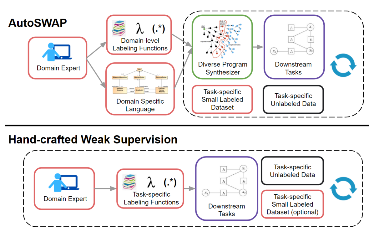
Figure 1: We present AutoSWAP, a framework for automatically synthesizing diverse sets of task-level labeling functions (LFs) with a small labeled dataset and domain knowledge encoded in domain-level LFs and a DSL. AutoSWAP significantly reduces labeler effort by automating LF generation.

Our Approach. We propose AutoSWAP (Automatic Synthesized WeAk SuPervision), a data-efficient framework for automatically generating task-level LFs using a novel diverse program synthesis formulation. As depicted in Figure 1, experts provide a domain-specific language (DSL) and domain-level LFs (LFs specific to a domain of tasks) for a given domain, such as mouse behaviors or vehicle motion planning. For each task to be studied in that domain, experts provide a small labeled dataset to specify the task, and AutoSWAP returns a set of structurally diverse task-level LFs that can be used in weakly supervised frameworks. The domain-level LFs (Figure 2) provide fine-grained, label-space agnostic “atomic instructions,” while the DSL contains abstract structural domain knowledge for composing the more general domain-level LFs into task-level LFs (Figure 3). The novel diversity cost enables AutoSWAP to generate structurally diverse LFs, which we and others empirically show outperform structurally homogeneous LFs in downstream tasks [33].

To the best of our knowledge, we are the first to demonstrate the effectiveness of program synthesis for automated LF generation. Existing works for generating LFs include iteratively selecting LFs by repeatedly querying experts for feedback [5] and training exponentially many simple heuristics models [33], which have limitations in scalability and tractability. In contrast, our approach represents domain knowledge in a DSL and domain-level LFs, which can then be used to automatically synthesize LFs for arbitrary tasks in a domain with our diverse program synthesizer.

We evaluate our approach in three behavior analysis domains with both sequential and nonsequential data: mouse [27], fly [14], and basketball player [36] behaviors. In these domains, data collection is expensive and new tasks frequently emerge, highlighting the importance of scalability. The datasets we use are based on agent trajectories, which provide low-dimensional inputs for easily creating domain-level LFs. We show that with existing expert defined domain-level LFs from [24, 14] and a simple DSL, AutoSWAP is capable of synthesizing high quality LFs with very little labeled data. These LFs outperform LFs from existing automatic weak supervision methods [33] and offer a data efficient approach to reducing domain expert effort.

To summarize, our contributions are:

• We propose AutoSWAP, which combines program synthesis with weak supervision to scalably and efficiently generate labeling functions.

• We propose a novel program-structural diversity cost that enables AutoSWAP to directly synthesize diverse sets of labeling functions, which we empirically show are more data efficient than purely optimal sets.

• We evaluate AutoSWAP in multiple behavior analysis domains and downstream tasks, and show that AutoSWAP is capable of significantly improving data efficiency and reducing expert cost.

Our implementation of AutoSWAP can be found at https://github.com/autoswap/autoswap_cvpr_2022.

2 Related Work

Behavior Analysis. In many domains, such as behavioral neuroscience [24, 19], sports analytics [36, 37], and traffic modeling [9], agent pose and location trajectory data is used for behavior analysis. This data is usually extracted from recorded videos using detectors and pose estimators [14, 24]; for example, we use trajectories from [24],  [14], and StatsPerform for our mouse, fly, and basketball datasets, respectively.

To accurately analyze this data for complex behaviors, frame-level behavior labels from domain experts are usually needed. However, annotating large datasets is time-consuming and monotonous [1], motivating methods for label-efficient modeling. For example, self-supervised learning [28] and unsupervised behavior discovery methods [3, 19, 6] aim to learn efficient behavior representations and discover new behaviors, respectively. Our work is complementary to these methods in that this is not a comparison between weak supervision and self-supervision. Rather, we evaluate the merits of our synthesized LFs in the context of weak supervision for learning expert-defined behaviors.

Weak Supervision. Weak supervision with LFs was introduced in the context of data programming [23]. Since then, LFs have been applied in a variety of settings, including for active learning [20, 4] and self-training [17] tasks. Our work is complementary to these works in that we automatically learn LFs that can be used as inputs to existing weakly supervised frameworks. We note that we are not the first to propose learning LFs from a small amount of training data. For example, IWS iteratively proposes rules and queries domain experts in a large-scale feedback loop [5]. More similar to our work, SNUBA [33] trains heuristics models, but does so without domain knowledge and has runtime exponential in the number of features. To the best of our knowledge, we are the first to apply program synthesis to this problem, and our framework outperforms existing model-based methods for learning LFs.

Program Synthesis. Traditionally, programming by example has been used to synthesize programs from a DSL that respect hard constraints on input/output examples [26, 15]. In recent years, a growing number of works have studied synthesizing programs with soft constraints, such as minimizing a loss function  [25, 13, 21, 31]. This relaxed form of program synthesis has been applied to a number of different domains including web information extraction [8], image structure analysis [12], and learning interpretable agent policies [34]. Of these works, algorithms that learn differentiable programs, such as [25], have shown great promise in being able to efficiently and simultaneously optimize program architectures and parameters. Here, we use concepts from differentiable program synthesis algorithms to synthesize diverse sets of LFs.

3 Methods

We introduce AutoSWAP, a framework for automatically generating diverse sets of task-level LFs. In our framework, domain experts provide a set of domain-level LFs and a DSL of useful relations. For each task to be studied, specified with a small labeled dataset, task-level LFs are automatically generated by the AutoSWAP diverse program synthesizer. These LFs can then be used in downstream applications involving weak supervision. In the following sections, we provide a background of key components in AutoSWAP (Section 3.1), detail the framework (Section 3.2), and describe example downstream applications (Section 3.3).

3.1 Background

⬇

# lambda_1 - whether fly is attacking target

def is_attacking(fly, tgt):

f2t_angle = atan((tgt.y - fly.y) / (tgt.x - fly.x))

rel_angle = |fly.abs_angle - f2t_angle|

return fly.speed > 2 and rel_angle < 0.1

# lambda_2 - ratio of fly wingspan

def wing_ratio(fly, tgt):

return quantize(fly.wing_x / fly.wing_y, 4)

# lambda_3 - fly speed relative to target speed

def relative_speed(fly, tgt):

return |fly.speed| / |tgt.speed|

Figure 2: Domain experts provide domain-level labeling functions, such as the ones above for the fly domain. Some domain-level LFs ($\lambda_{1}$, $\lambda_{2}$) label for specific tasks (and would be considered task-level LFs on their own), while others ($\lambda_{3}$) return features.

Domain-level Labeling Functions. In weak supervision, users provide a set of task-level hand-crafted heuristics called labeling functions (LFs). LFs can be noisy and abstain from labeling, but LFs must output in downstream task’s label space $\mathcal{Y}$. We relax this requirement in AutoSWAP by allowing domain experts to provide domain-level LFs (Figure 2). These LFs do not have to output in $\mathcal{Y}$, which reduces LF creation overhead and allows for more expressive LFs. This also allows us to reuse LFs across multiple tasks within the same domain, aiding scalability.

Domain Specific Languages. Domain specific languages (DSLs) define the allowable submodules and structures in synthesized programs, and are a key component of program synthesis algorithms. Many recent works have adopted purely functional DSLs [25], where DSL items are functions that output to the input space of other DSL items or the final output space. In AutoSWAP, domain experts provide a purely functional DSL with program structures that may be useful in generated LFs. We show empirically that even using a very simple DSL in AutoSWAP can result in significant reductions in expert effort.

Differentiable Program Synthesis via Neural Completions and Guided Search. Our program synthesis formulation is based on NEAR, which finds $\epsilon$-optimal differentiable programs using admissible search heuristics [16, 25]. While NEAR is one instantiation of AutoSWAP, our diverse synthesis formulation (Section 3.2) is theoretically compatible with any search-based synthesizer. Here, the DSL $\mathcal{D}$ is a context-free grammar with differentiable variables. Programs are defined by a program architecture $\alpha$ in the context-free language of $\mathcal{D},\mbox{CFL}_{\mathcal{D}}$, and a set of real parameters $\theta$, and are denoted by $[\![\alpha]\!](x,\theta):\mathcal{X}\rightarrow\mathcal{Y}$. Synthesizing a program that is optimal w.r.t. a cost function $F$ and dataset $(X,Y)\in(\mathcal{X},\mathcal{Y})$ is equivalent to

$$(\alpha^{*},\theta^{*})=\operatorname*{arg\,min}_{\alpha,\theta}F([\![\alpha]\!](X,\theta),Y).$$ (1)

To find $(\alpha^{*},\theta^{*})$, we search over $\mbox{CFL}_{\mathcal{D}}$. This search space is a tree $\mathcal{G}$, where the root node is an empty architecture, interior nodes are incomplete architectures (architectures with unknown components), and leaf nodes are complete architectures. Edges in $\mathcal{G}$ represent single productions from $\mathcal{D}$ between two architectures. We bound the search tree by limiting the search depth to $m$ and “completing” incomplete architectures by substituting unknown components with neural networks (“neural completions”).

Since neural completions are differentiable, the minimum cost-to-go (CTG) w.r.t. $F$ of a neural completion can be computed by optimizing the neural completion’s parameters. Furthermore, this minimum CTG of a neural completion is an $\epsilon$-admissible heuristic[16] for the true CTG of the corresponding incomplete architecture (proof in [25]). This allows us to use informed search algorithms on $\mathcal{G}$ to find $\epsilon$-optimal solutions to Equation 1.

3.2 AutoSWAP

Synthesizing Diverse Sets of Programs. Diverse sets of LFs have been shown to improve data efficiency relative to purely optimal sets in downstream applications of weak supervision [33]. This is partly due to diverse sets having improved label coverage (fewer data points where all LFs abstain) [33], and from having more learning signals for the downstream model [29]. The program synthesizer in Section 3.1 can be run repeatedly to obtain a set of purely optimal LFs, but there is no guarantee that the set will be diverse. Here, we introduce a structural diversity cost and admissible heuristic that allows for direct synthesis of diverse sets of programs using informed search algorithms. We empirically show that using the diversity cost improves performance, corroborating [33]’s observations.

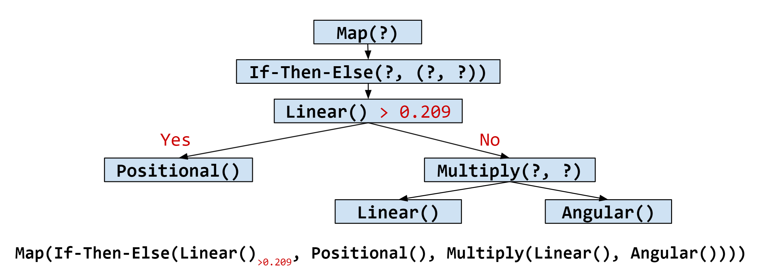
Figure 3: A complete program and its tree representation. Each ‘?’ represents one child node function. The depicted program is an actual AutoSWAP LF for the “lunge vs. no behavior” in the Fly domain. The program can be interpreted as “If the linear speed between the flies is small, classify the angular domain-level LFs of the flies. Otherwise, classify the product of transformations of the linear speed and positional domain-level LFs.” Note the parameters (red) are not included in the structural diversity cost.

Consider a complete program $P$, which is a composition of variables in $\mathcal{D}$. By construction of $\mathcal{G}$, we can convert $P$ to a tree $T_{P}$ where each node is a variable in $P$ and a node’s children are its input variables (Figure 3). Then, given a set of complete programs $\mathcal{P}$ and a complete program $P$, we define the structural cost $C_{P,\mathcal{P}}$ of $P$ relative to $\mathcal{P}$ as:

$$\frac{1}{C_{P,\mathcal{P}}}=q\Big{(}\frac{1}{\|\mathcal{P}\|}\sum_{P^{\prime}\in\mathcal{P}}\mathtt{ZSS}(T_{P},T_{P^{\prime}})\Big{)},$$ (2)

where $q:\mathbb{R}\to\mathbb{R}$ is a user defined monotonically increasing function and $\mathtt{ZSS}$ is the Zhang-Shasha tree edit distance (TED) [38]. Essentially, programs with a higher average TED to the elements of $\mathcal{P}$ incur a lower diversity cost.

Since this structural cost is not defined for incomplete programs or neural completions, $C_{P,\mathcal{P}}$ cannot be used in informed search algorithms. However, the following admissible heuristic $H_{P_{I},\mathcal{P}}$ for incomplete programs $P_{I}$ allows us to create a set of diverse programs by iteratively synthesizing programs and adding them to $\mathcal{P}$.

Lemma 3.1.

Let $P_{I}$ be an incomplete program and $T_{P_{I}}$ be the tree of its known variables. $T_{P_{I}}$ is guaranteed to exist by construction of $\mathcal{G}$. Define $H_{P_{I},\mathcal{P}}$ as:

$$U_{P_{I},P^{\prime}} =m-\|P_{I}\|+\mathtt{ZSS}(T_{P_{I}},T_{P^{\prime}}),$$

$$\frac{1}{H_{P_{I},\mathcal{P}}} =q\Big{(}\frac{1}{\|P\|}\sum_{P^{\prime}\in\mathcal{P}}U_{P_{I},P^{\prime}}\Big{)},$$

where $\|P_{I}\|$ is the number of known variables in $P_{I}$. $H_{P_{I},\mathcal{P}}$ is an admissible heuristic for the CTG from $P_{I}$ in $\mathcal{G}$.

Proof.

Consider $U_{P_{I},P^{\prime}}$. $m-\|P_{I}\|$ is an upper bound on the TED between $T_{P_{I}}$ and the tree of any complete descendant $P^{*}$ of $P_{I}$ in $\mathcal{G}$. From the triangle inequality,

$$U_{P_{I},P^{\prime}} =m-\|P_{I}\|+\mathtt{ZSS}(T_{P_{I}},T_{P^{\prime}})$$

$$\geq\mathtt{ZSS}(T_{P_{I}},T_{P^{*}})+\mathtt{ZSS}(T_{P_{I}},T_{P^{\prime}})$$

$$\geq\mathtt{ZSS}(T_{P^{*}},T_{P^{\prime}}).$$

Then, as TEDs are nonnegative, $m\geq\|P_{I}\|$, and $q$ is nondecreasing, $H_{P_{I},\mathcal{P}}\leq C_{P^{*},\mathcal{P}}$. Thus, $H$ a admissible heuristic for the structural CTG from $P_{I}$. ∎

AutoSWAP Framework. AutoSWAP uses program synthesis to automate significant parts of the weak supervision pipeline and reduce domain expert effort. Domain experts provide a set of domain-level LFs $\Lambda_{m}=\{\lambda_{i}:\mathcal{X}\to\mathcal{Y}_{i}\}$, a purely functional DSL $\mathcal{D}$, and a small labeled dataset $(X,Y)\in(\mathcal{X},\mathcal{Y})$ to specify tasks within the domain. In order to use $\Lambda_{m}$ when synthesizing programs with $\mathcal{D}$, all $\lambda_{i}$ must be added to $\mathcal{D}$. This can be done either by implementing each $\lambda_{i}$ with operations from $\mathcal{D}$, or precomputing and selecting $\Lambda_{m}(X)$ as input features in $\mathcal{D}$; we do the latter in our experiments. With $\mathcal{D}$, AutoSWAP runs the diverse program synthesis algorithm $n$ times to generate a set $\Lambda$ of $n$ LFs. $\Lambda$ can then be used in downstream tasks, such as in weak supervision label models to generate weak labels. See Algorithm 1 for a detailed description of AutoSWAP.

Input: $\Lambda_{m}$, $\mathcal{D}$, labeled dataset $D_{L}$, # LFs $n$

Output: task-level LFs $\Lambda$

$\mathcal{D}\leftarrow$ Combine $\Lambda_{M}$ and $\mathcal{D}$

$\mathcal{P}\leftarrow\emptyset$

while $\|\mathcal{P}\|\leq n$ do

       Synthesize $P$ with $\mathcal{D},D_{L},\mathcal{P}$

       $\mathcal{P}\leftarrow\mathcal{P}\cup\{P\}$

end while

$\Lambda\leftarrow\mathcal{P}$, return $\Lambda$.

Algorithm 1 AutoSWAP.

3.3 Downstream Tasks

We describe two downstream tasks in which weak labels can be used. These examples, which our experiments are based on, are just a subset of the many weakly supervised learning frameworks in existence such as ASTRA [17].

Active Learning. Active learning is a paradigm where the learning algorithm can selectively query for new data to be labeled. Here, we use labels from task-level LFs as additional features for a downstream classifier. The downstream classifier’s predictions are used to select data for labeling. To evaluate generated LFs in active learning settings, we consider the performance of downstream classifiers at multiple data amounts. Given a sorted list $A$ of data amounts, at each amount we generate new LFs, train a downstream classifier, and select data points for labeling to form the next batch. An exact description of our active learning setup for AutoSWAP can be found in Algorithm 2.

Input: $\Lambda_{m},\mathcal{D},n$, unlabeled $X_{U}$, $A$.

Sort $A$ in increasing order.

Randomly select $A_{1}$ points $X_{L}$ from $X_{U}$.

$X_{U}\leftarrow X_{U}\setminus X_{L}$

$Y_{L}\leftarrow$ Obtain labels for $X_{L}$.

for $i=1,...,\|A\|-1$ do

       $\Lambda_{i}\leftarrow$ AutoSWAP($\Lambda_{m},\mathcal{D},(X_{L},Y_{L}),n$).

       $X^{\prime}_{L}\leftarrow\begin{bmatrix}X_{L}&\Lambda_{i}(X_{L})\end{bmatrix}$

       Train downstream classifier $C_{i}$ with $(X^{\prime}_{L},Y_{L})$.

       Select $A_{i+1}-A_{i}$ points $X^{\prime}_{L}$ using max entropy uncertainty sampling.

       $X_{U}\leftarrow X_{U}\setminus X^{\prime}_{L}$

       $X_{L}\leftarrow X_{L}\cup X^{\prime}_{L}$

       $Y_{L}\leftarrow Y_{L}\cup\{\mbox{Obtain labels for }X^{\prime}_{L}\}$

end for

Algorithm 2 AutoSWAP for Active Learning.

Weak Supervision. Weak supervision frameworks generally depend on a generative label model weakly label unlabeled samples. Using no ground truth labels, the generative model produces probabilistic estimates (“weak labels”) for the true labels $Y_{U}$ of an unlabeled set $X_{U}$ by modeling the LF outputs $\Lambda(X_{U})$. Weakly labeled data can then be used to augment labeled datasets in downstream tasks.

To evaluate AutoSWAP in weak supervision settings, we start with a small labeled dataset $D_{L}$ and a list of unlabeled data amounts $A$. LFs are generated using the small labeled dataset and abstain using the method in [33]. Then, weak labels are generated from these LFs for all unlabeled data using the generative model. For each data amount $A_{i}\in A$, a random set $D_{PL}$ of $A_{i}$ weakly labeled data points is selected and the performance of a downstream classifier is measured using the training set $D_{L}\cup D_{PL}$. An exact description of our weak supervision setup is in Algorithm 3.

Input: $\Lambda_{m},\mathcal{D},n$, Labeled $(X_{L},Y_{L})$, Unlabeled $X_{U}$, $A$.

$\Lambda\leftarrow$ AutoSWAP($\Lambda_{m},\mathcal{D},(X_{L},Y_{L}),n$).

$\Lambda\leftarrow\mbox{Abstain}(\Lambda)$ [33]

Sort $A$ in increasing order.

for $i=1,...,\|A\|$ do

       Randomly select $A_{i}$ points $X_{P}$ from $X_{U}$.

       $X^{\prime}_{L}\leftarrow X_{L}\cup X_{P}$

       $Y^{\prime}_{L}\leftarrow Y_{L}\cup\Lambda(X_{P})$

       Train downstream classifier $C_{i}$ with $(X^{\prime}_{L},Y^{\prime}_{L})$.

      

end for

Algorithm 3 AutoSWAP for Weak Supervision.

4 Experiments

We evaluate AutoSWAP in multiple real world behavior analysis domains (Section 4.1), and show that our framework outperforms existing LF generation methods in weak supervision and active learning settings (Section 5.1). Since researchers often study multiple behaviors in a domain [24, 14], we consider each behavior its own task.

4.1 Datasets

We use datasets from behavioral neuroscience (mouse and fly behaviors) as well as sports analytics (basketball player trajectories). These datasets include rare behaviors, multi-behavior tasks, and sequential data, making them good representations of real-world behavior analysis tasks. Each dataset contains a train, validation, and test split; the validation split is only used for model checkpoint selection.

Fly vs. Fly (Fly). The fly dataset [14] contains frame-level annotations of videos of interactions between two fruit flies. Our train, validation, and test sets contain 552k, 20k, and 166k frames. We use fly trajectories tracked by FlyTracker [14] and evaluate on 6 behaviors: lunge, wing threat, tussle, wing extension, circle, copulation. This is a multi-label dataset and we report the mean Average Precision (mAP) over binary classification tasks for each behavior. All behaviors except for copulation are rare; lunge, wing threat, and tussle occur in $<5\%$ of frames, and wing extension and circle occur in $<1\%$ of frames. The domain-level LFs for this dataset are based on features from [14].

CalMS21 (Mouse). The CalMS21 dataset [27] consists of frame-level pose and behavior annotations from videos of interactions between pairs of mice. We use data from Task 1 (532k train, 20k validation, 119k test) and evaluate on a set of 3 behaviors: attack, investigation, and mount. These behaviors are mutually exclusive and we report the mAP over these classes. We use a subset of the features in  [24] as domain-level LFs for this dataset.

Basketball. The Basketball dataset, also used in [36, 25, 37], contains sequences of basketball player trajectories from Stats Perform (18k train, 1k validation, 2.7k test). Labels for which offense player (5 total) had the ball for the majority of the sequence were extracted with  [2]. We perform sequential classification in downstream tasks, and report the mAP over each offense player vs. the other 4. Our domain-level LFs include player acceleration, velocity, and position among others. We exclude information about the ball position in the domain-level LFs and data features to focus on analyzing player behaviors.

4.2 Baselines

We compare AutoSWAP to two main baselines: student networks from student-teacher training and decision trees from SNUBA [33]. We show that AutoSWAP outperforms both in data efficiency, requiring a fraction of the data to achieve or exceed performance parity. For both baselines, domain-level LFs are incorporated as input features to evaluate the effectiveness of AutoSWAP and not the domain-level LFs themselves. We do not compare against IWS [5], as IWS is a human-in-the-loop LF generation system. We also do not compare against ASTRA [17], as ASTRA is a weak supervision framework for using task-level LFs in self training. However, ASTRA can be used as a downstream task for AutoSWAP.

Student Networks Student-teacher training (from knowledge distillation[35]) has been used successfully in self-training. We adopt the concept of student networks by training models with similar capacity as the downstream classifier to serve as LFs. In weak supervision experiments, these student LFs and the label model (Equation 3) serve as a teacher model for the downstream classifier.

Decision Trees and SNUBA Decision trees have been shown to be good LFs [33] and offer some degree of interpretability. The SNUBA framework [33] generates a diverse set of decision tree LFs by training $2^{k}-1$ decision trees over all feature subsets and then pruning trees based on a diversity and performance metric, where $k$ is the feature dimension of $\mathcal{X}$. Clearly, this is intractable for large $k$, which is often the case for behavior analysis tasks. Furthermore, SNUBA does not use domain knowledge, instead relying on the complete set of decision trees for data efficiency. In relation to SNUBA, AutoSWAP can be viewed as an scalable alternative to the synthesizer and pruner stages.

4.3 Training Setup

Our experimental setup consists of two stages: obtaining LFs, and evaluating generated LFs in downstream tasks. Our downstream tasks include active learning, where LFs are used to select data for labeling, and weak supervision, where LFs generate pseudolabels for unlabeled data points.

4.3.1 Obtaining labeling functions

Synthesized Programs via AutoSWAP. For each domain, we use a simple DSL that includes add, multiply, fold, and differentiable if-then-else (ITE) structures among others. We synthesize programs with our diverse program synthesizer and A^∗ search. Our cost function is the sum of the $F_{1}$ cost from [25] and our diversity cost $C_{P,\mathcal{P}}$. We set $q(x)$ to $x^{2}$ and $m$ to $\log_{2}{\|\Lambda_{m}\|}$. Program parameters are trained with weighted cross entropy loss. More information about the exact DSL used is in the Supplementary Materials.

Student Networks. We use neural networks for frame classification tasks and LSTMs for scene classification tasks. To induce diversity in the learned student networks, we take inspiration from [35] and randomly set the size of each layer so the “expected” student network is of similar capacity as the downstream classifier. All student networks are trained using weighted cross entropy loss.

Decision Trees. We fit decision trees using Gini impurity as the split criteria. We limit the depth of decision trees to $\log_{2}{k}$, so the number of nodes is $O(k)$. We select diverse sets of decision trees by pruning a superset of trees based on coverage and performance, similar to how SNUBA does[33]. However, unlike SNUBA, we group our features when generating the superset, as training $2^{k}-1$ decision trees is intractable with our datasets.

4.3.2 Downstream Tasks

We use 3 LFs in our main experiments. Experiments with more LFs (5, 7) are in the Supplementary Materials.

Active Learning. As previous described, we evaluate the performance of AutoSWAP at multiple data amounts, selecting additional labeled data with active learning at each amount (Algorithm 2). We use max-entropy uncertainty sampling on downstream classifier outputs to select points for labeling [18]. We use $\{$1000, 2000, 3500, 5000, 7500, 12500, 25000, 50000$\}$ frames for the fly and mouse datasets and $\{$500, 1000, 1500, 2000, 3000, 4000, 5000$\}$ sequences for the basketball dataset.

Weak Supervision. In our weak supervision experiments, we use factor graph model proposed in [23, 22].

$$p_{\theta}(Y_{U},\Lambda)=Z_{\theta}^{-1}\exp\Big{(}\sum_{i=1}^{\|X_{U}\|}\theta^{T}\phi_{i}(\Lambda(X_{U_{i}}),Y_{U_{i}})\Big{)}.$$ (3)

Here, LF accuracies are modeled by factor $\phi_{i,j}^{Acc}(\Lambda,Y_{U})=\mathbb{1}\{\Lambda_{j}(X_{U_{i}})=Y_{U_{i}}\}$, and the proportion of data the LF labels is modeled by $\phi_{i,j}^{Lab}(\Lambda,Y_{U})=\mathbb{1}\{\Lambda_{j}(X_{U_{i}})\neq\emptyset\}$.

For the labeled dataset, we use 2000 frames for the fly and mouse datasets, and 500 sequences for the basketball dataset. Our unlabeled data amounts are set to $\{1\times,2\times,3\times,4\times,5\times\}$ the number of labeled points.

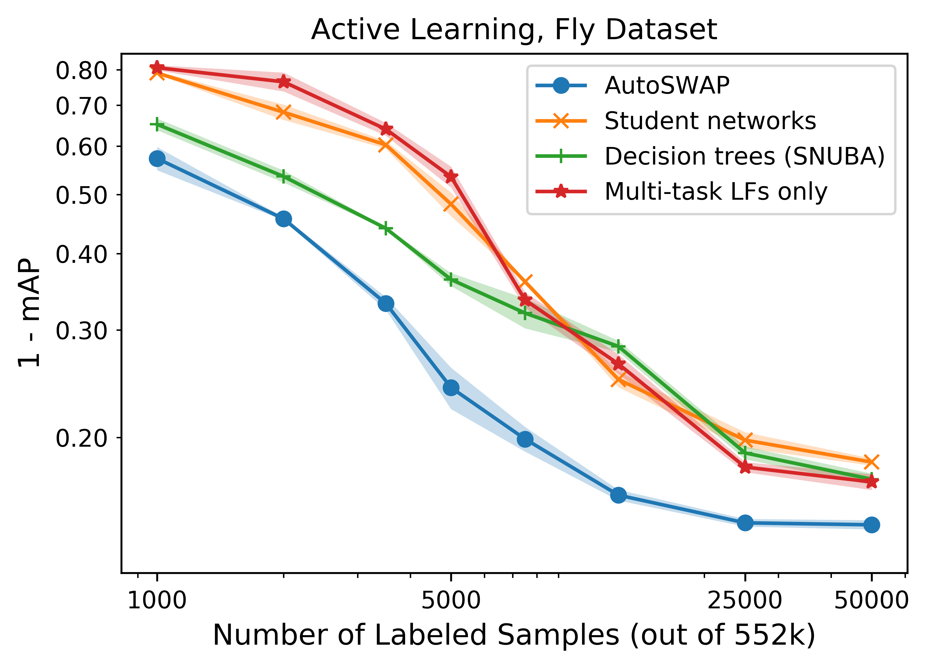
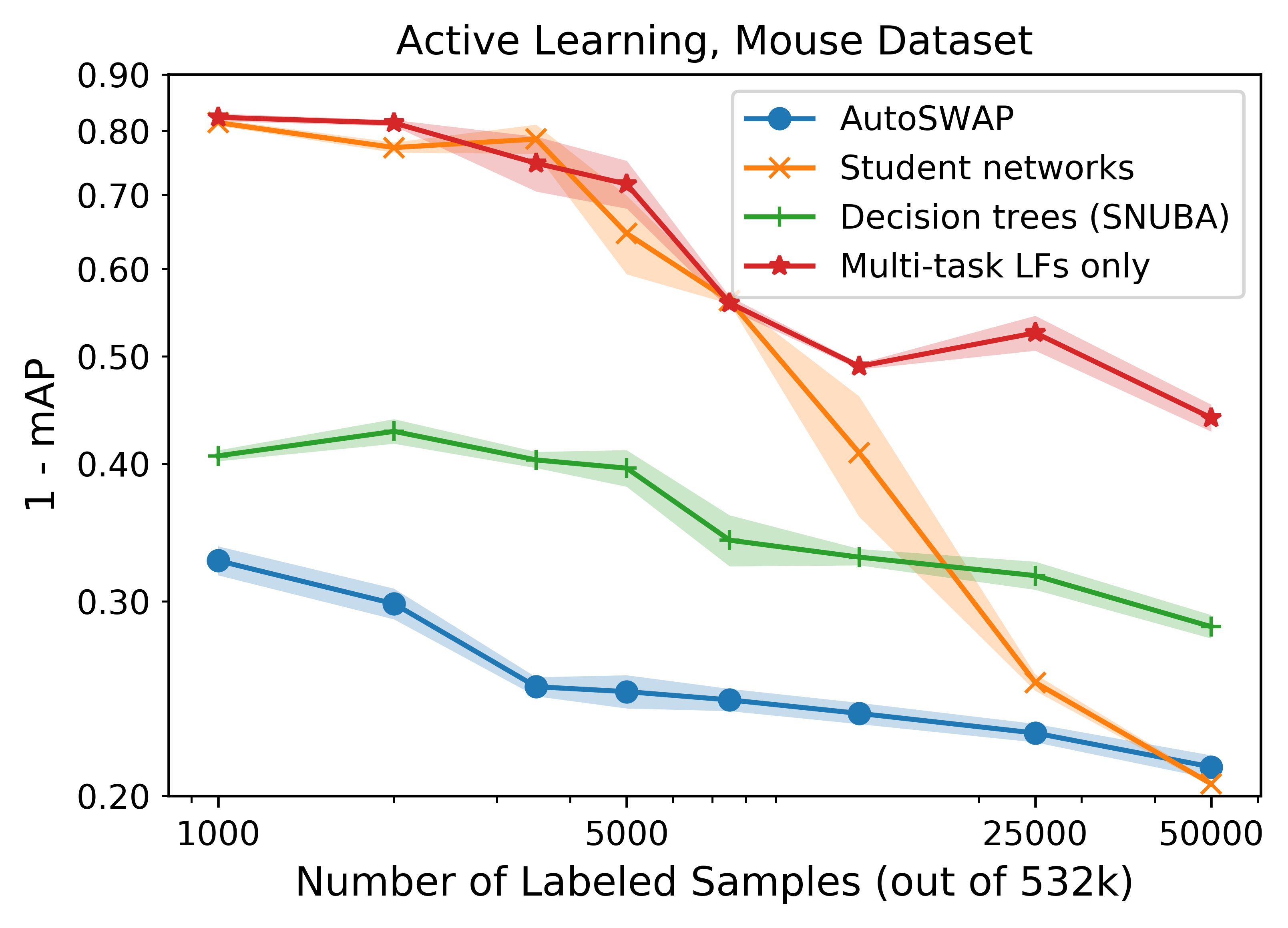
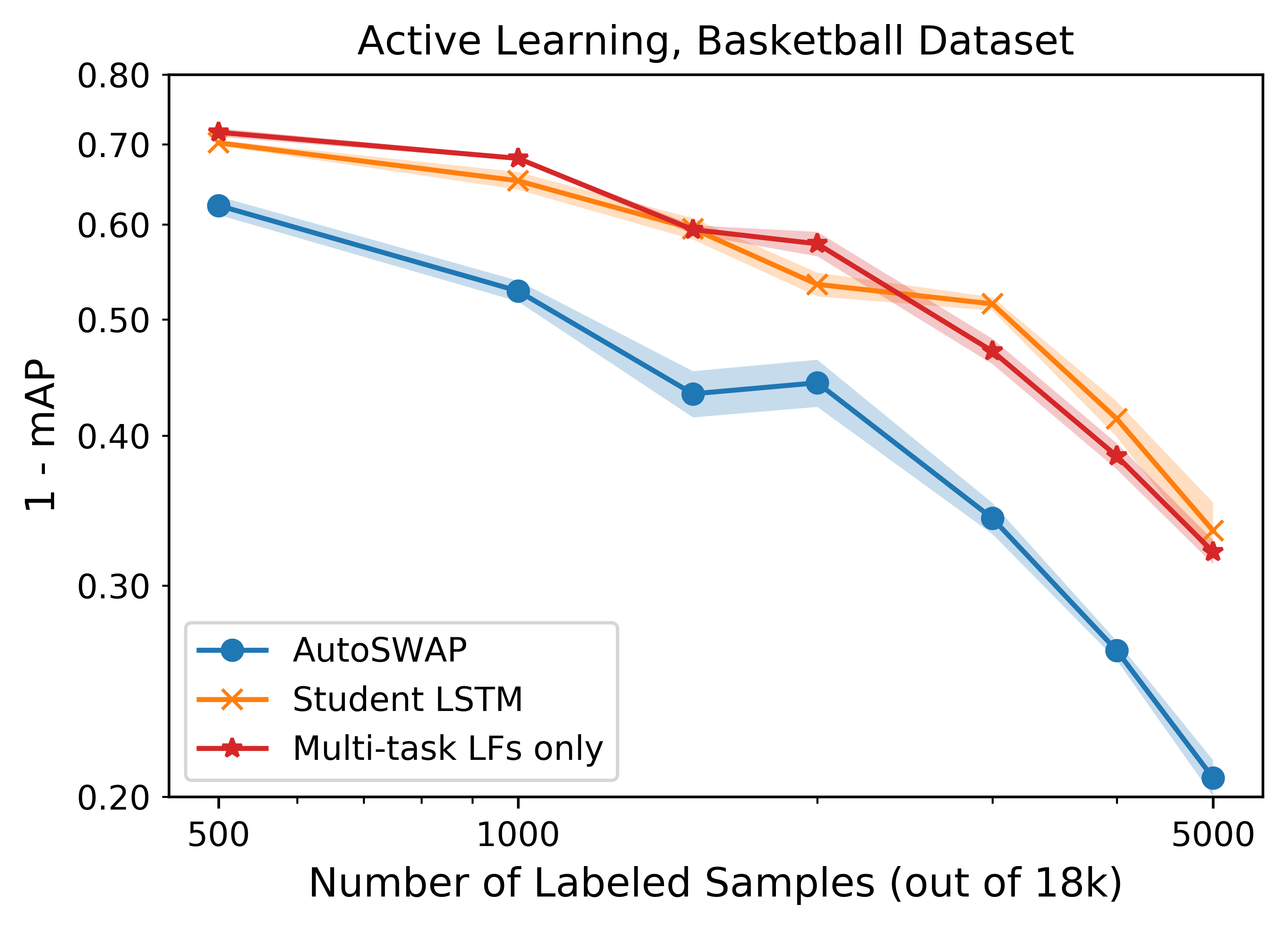
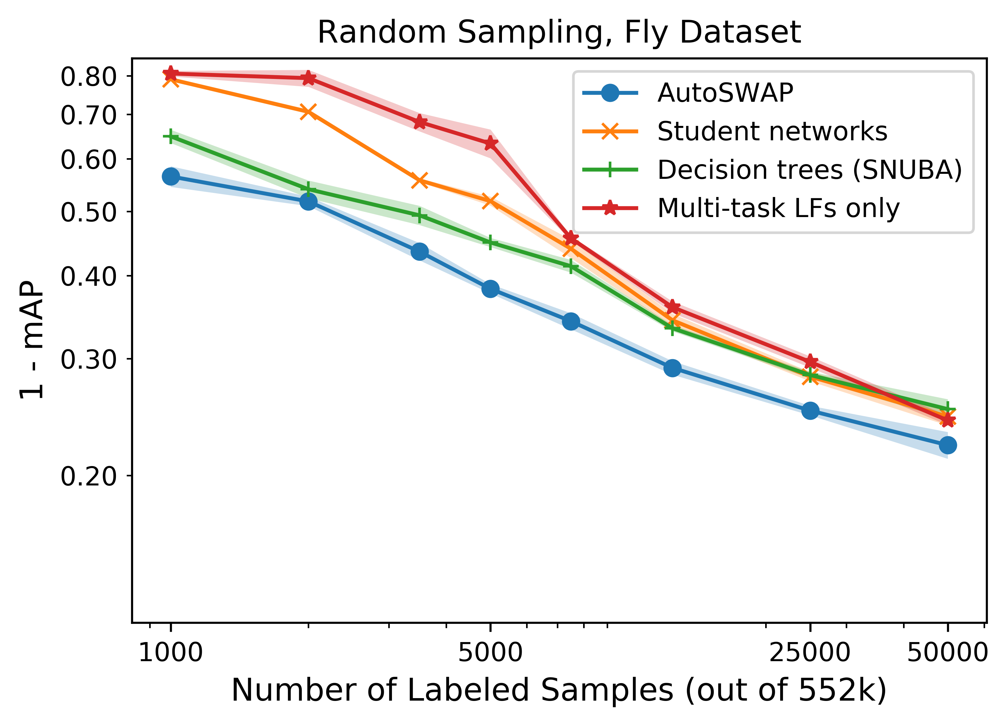
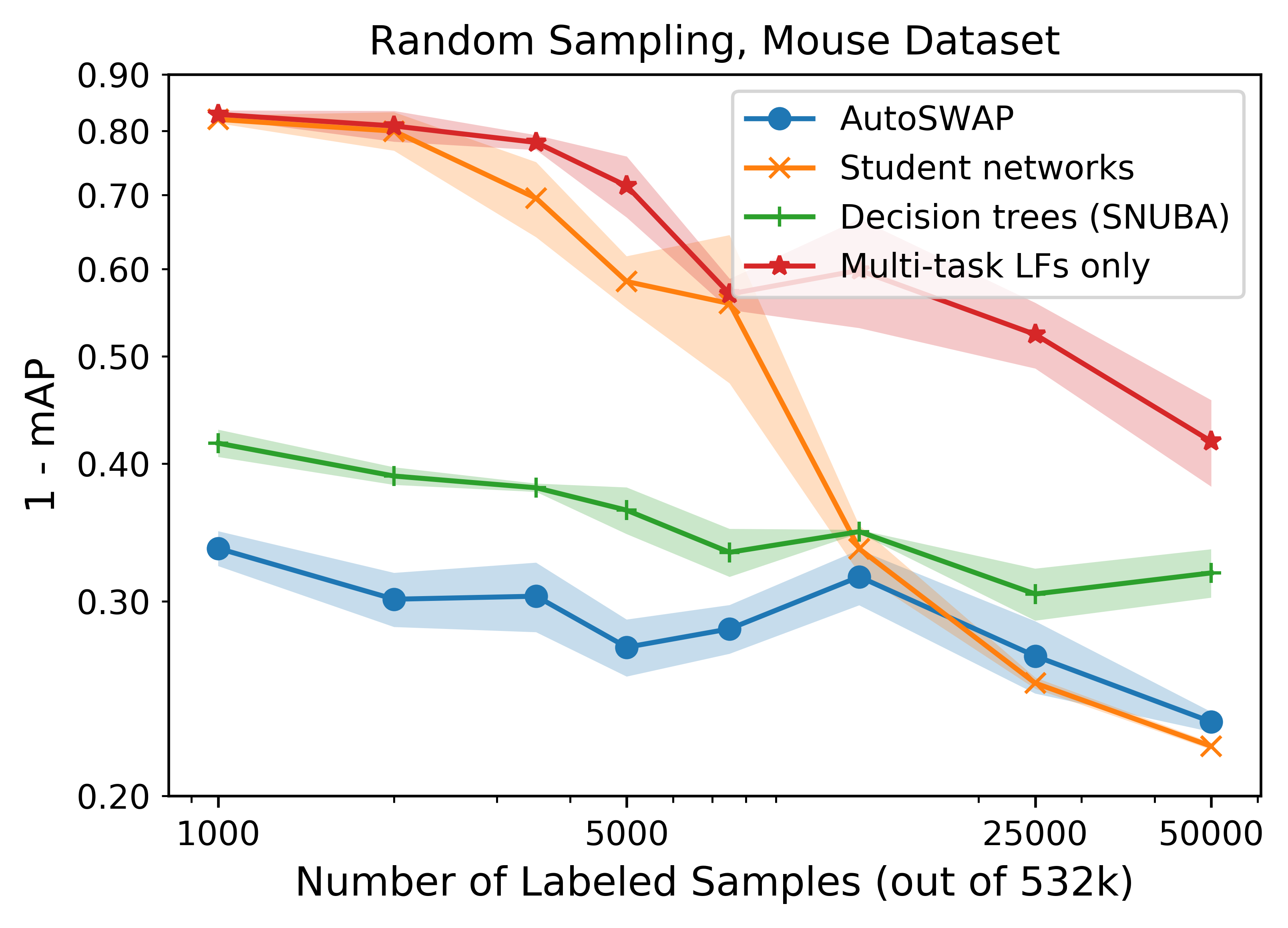
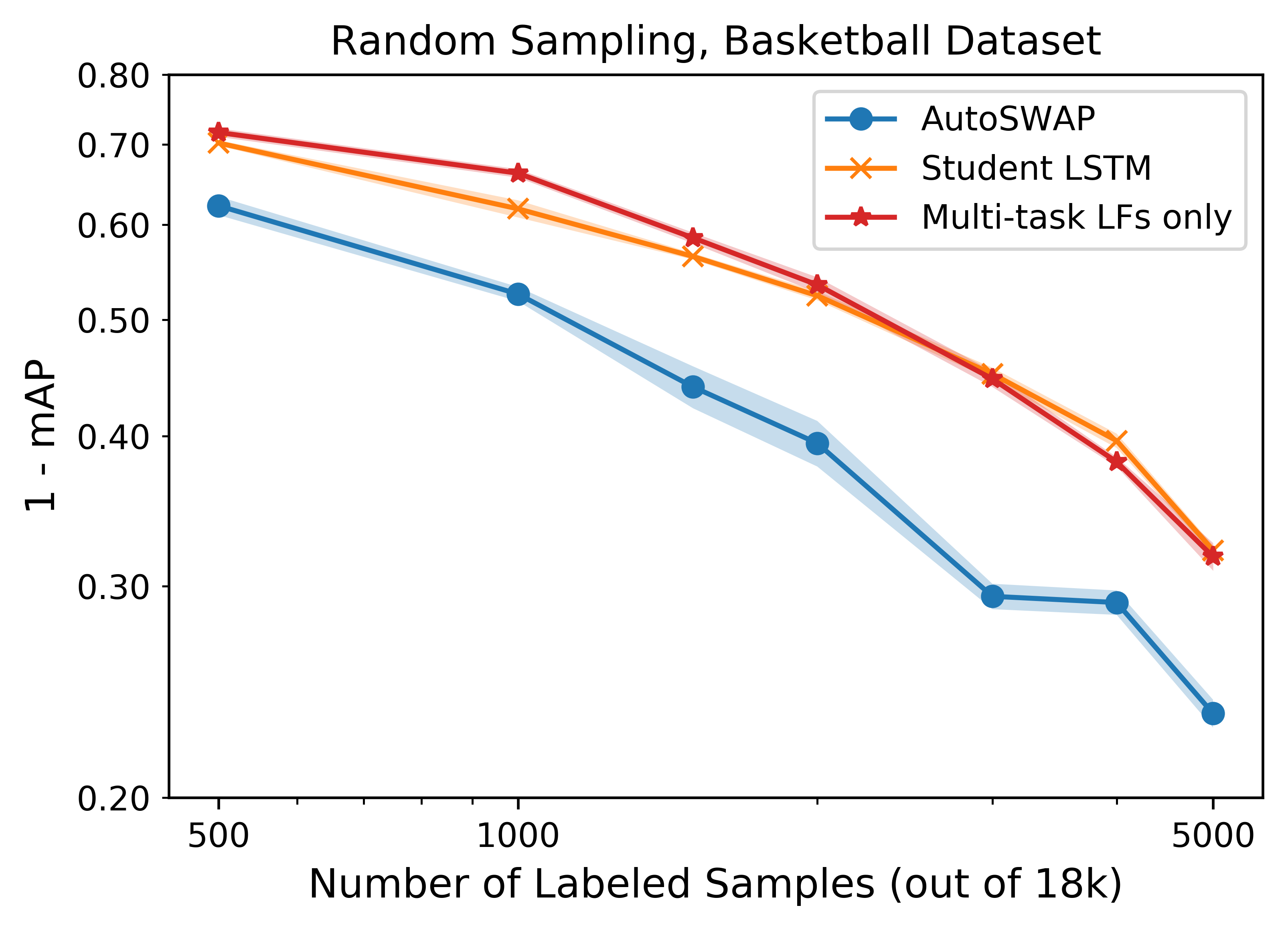
Figure 4: AutoSWAP Active Learning Experiments. Each line represents the mean of 5 random seeds for an automatic labeling function method. The shaded region is the standard error of the seeds. As can be seen, AutoSWAP matches or outperforms all baseline methods using only a fraction of the data. Note that all plots are on log-log scales.

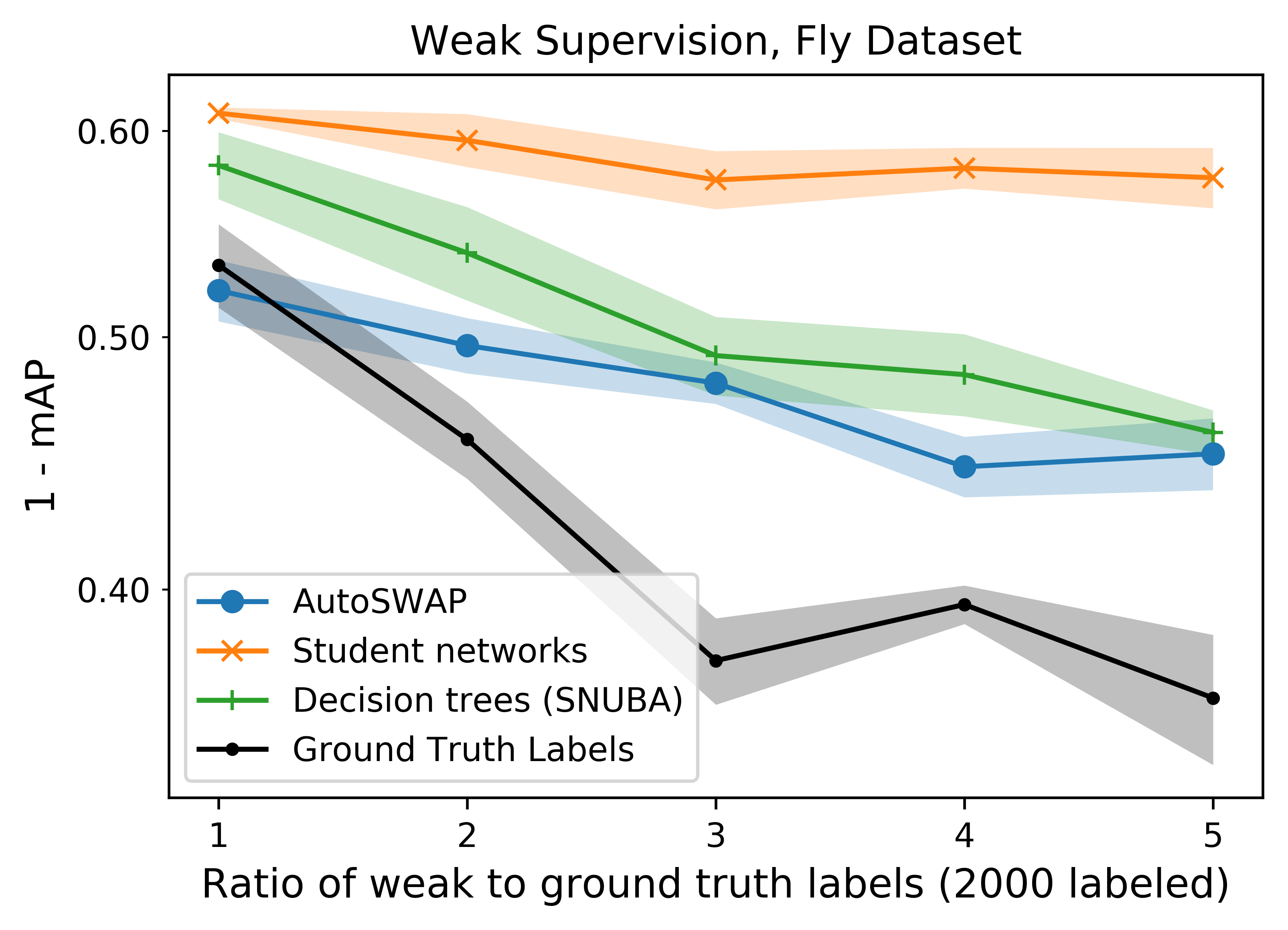
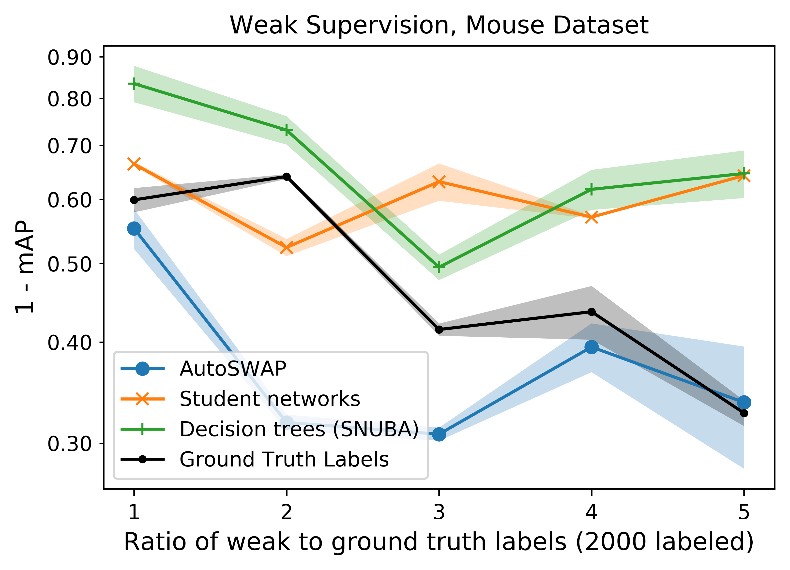
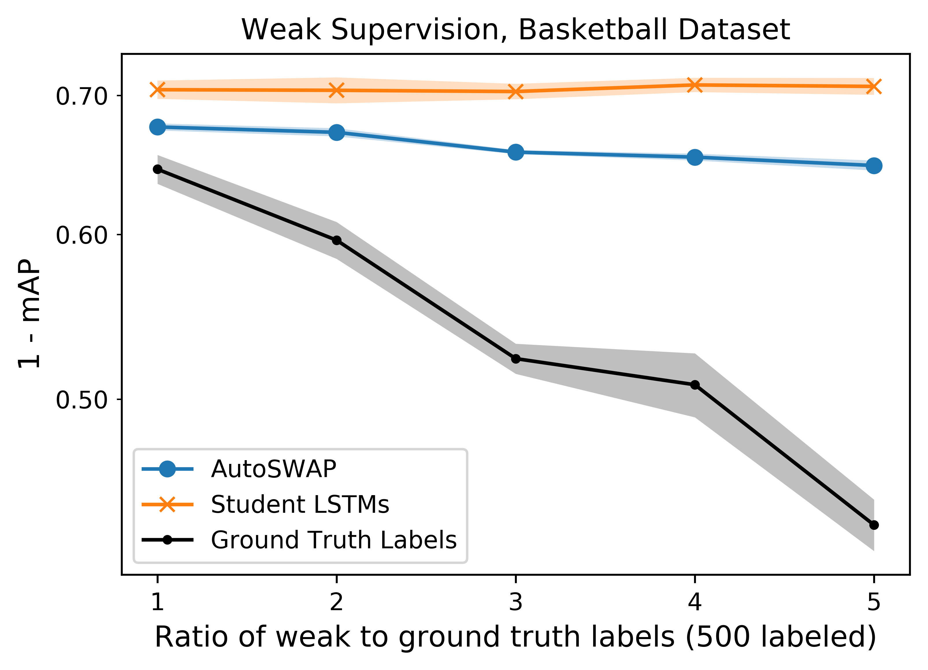
Figure 5: AutoSWAP Weak Supervision Experiments. Each line represents the mean of 5 random seeds for an automatic labeling function method. The shaded region is the standard error of the seeds. The gray line shows performance when ground truth labels are used as weak labels. Although it may seem odd that AutoSWAP outperforms ground truth labels in the Mouse dataset, weak labels have been observed to outperform ground truth labels in other works [17]. Note that all plots are on log-log scales.

5 Results

We compare the data efficiency of AutoSWAP against the baselines on our behavior analysis datasets. We do not run the decision tree (SNUBA) baseline on the Basketball dataset as it contains only sequential data.

5.1 Data Efficiency Results

Active Learning. AutoSWAP LFs are far more data efficient than baseline methods across all datasets, indicating that AutoSWAP is effective in reducing label cost in active learning settings (Figure 4). This difference is especially pronounced in the Mouse dataset, where AutoSWAP achieves parity with decision tree LFs with roughly 30$\times$ less data. In the Fly dataset, AutoSWAP is consistently $\sim 4\times$ more data efficient than the baselines, and no baseline is able to reach performance parity with AutoSWAP by 50000 samples (9.1% of the entire Fly dataset). We observe a similar trend in the Basketball dataset, with AutoSWAP being $\sim 2\times$ as data efficient. We also observe an improvement in data efficiency even when using random sampling, and note that uncertainty sampling widens the gap between AutoSWAP and the baselines.

While AutoSWAP LFs themselves do not necessarily perform better than baseline LFs when evaluated on their own (see the Supplementary Materials), they do provide a stronger learning signal for downstream classifiers than the baselines. These data efficiency differences can be attributed in part the structural domain knowledge encoded in the DSL, as the domain-level LFs themselves perform significantly worse. For example, a AutoSWAP LF classifying “lunge vs. no behavior” for the Fly dataset can be seen in Figure 3, and the structure of this program cannot be easily approximated with a decision tree or a neural network.

Weak Supervision. Similar to our active learning experiments, we observe that AutoSWAP is more data efficient than the baselines in weak supervision settings (Figure 5). We note that the ground truth labels are not a baseline in this setting, as they are essentially an “optimal” case where the weak labels match the ground truth labels.

On the Fly dataset, AutoSWAP generally performs better than both baselines, and on the Mouse and Basketball datasets, no baseline is able to match the performance of AutoSWAP LFs at any evaluated amount of annotated data. AutoSWAP is even able to outperform the ground truth labels in the Mouse dataset at some levels of annotated data, which indicates that the learned LFs are especially informative. Finally, we observe that AutoSWAP generally improves with more weakly labeled data points, which is useful as there is no expert annotation cost to using more weakly labeled data points.

5.2 Additional Results

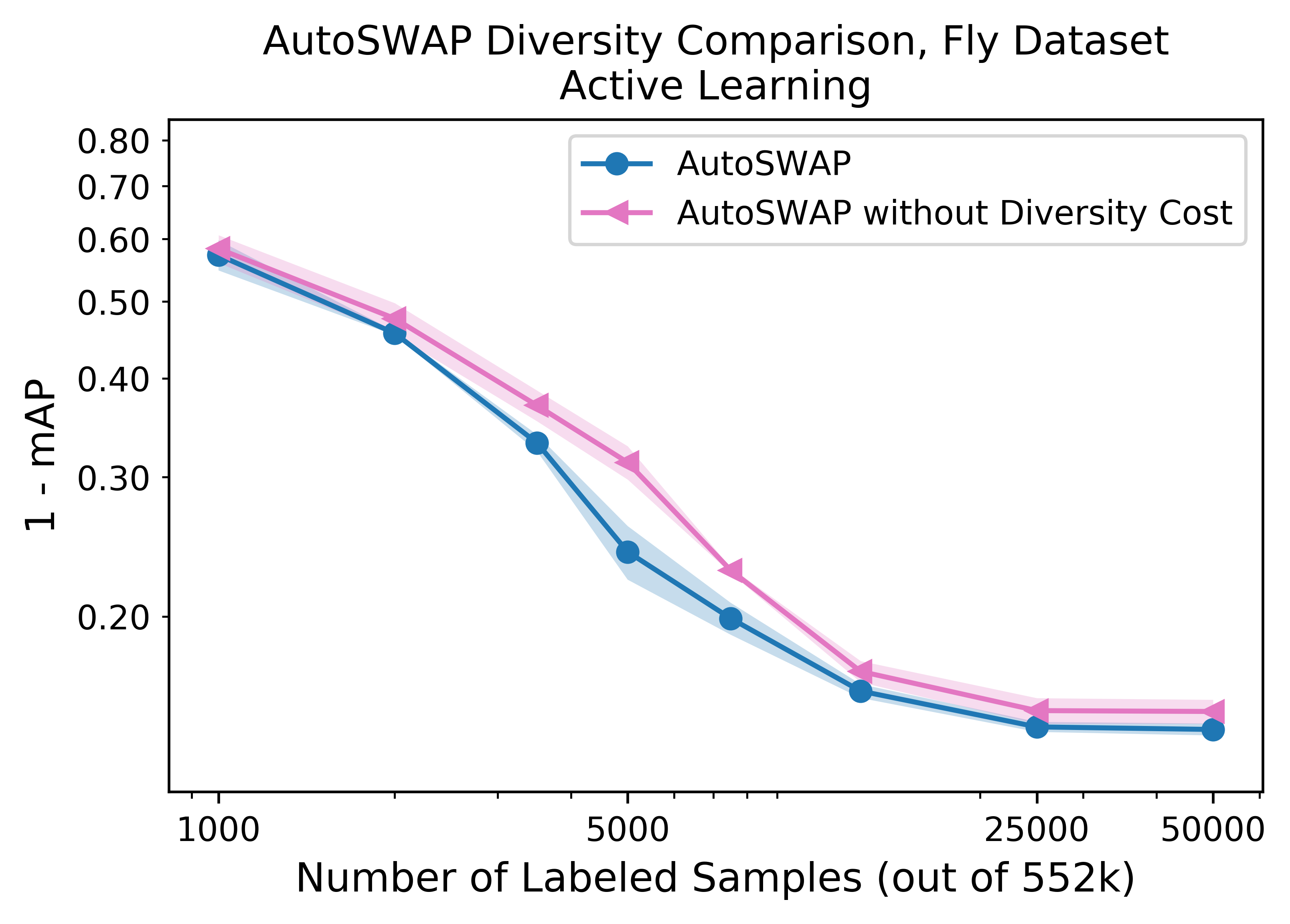
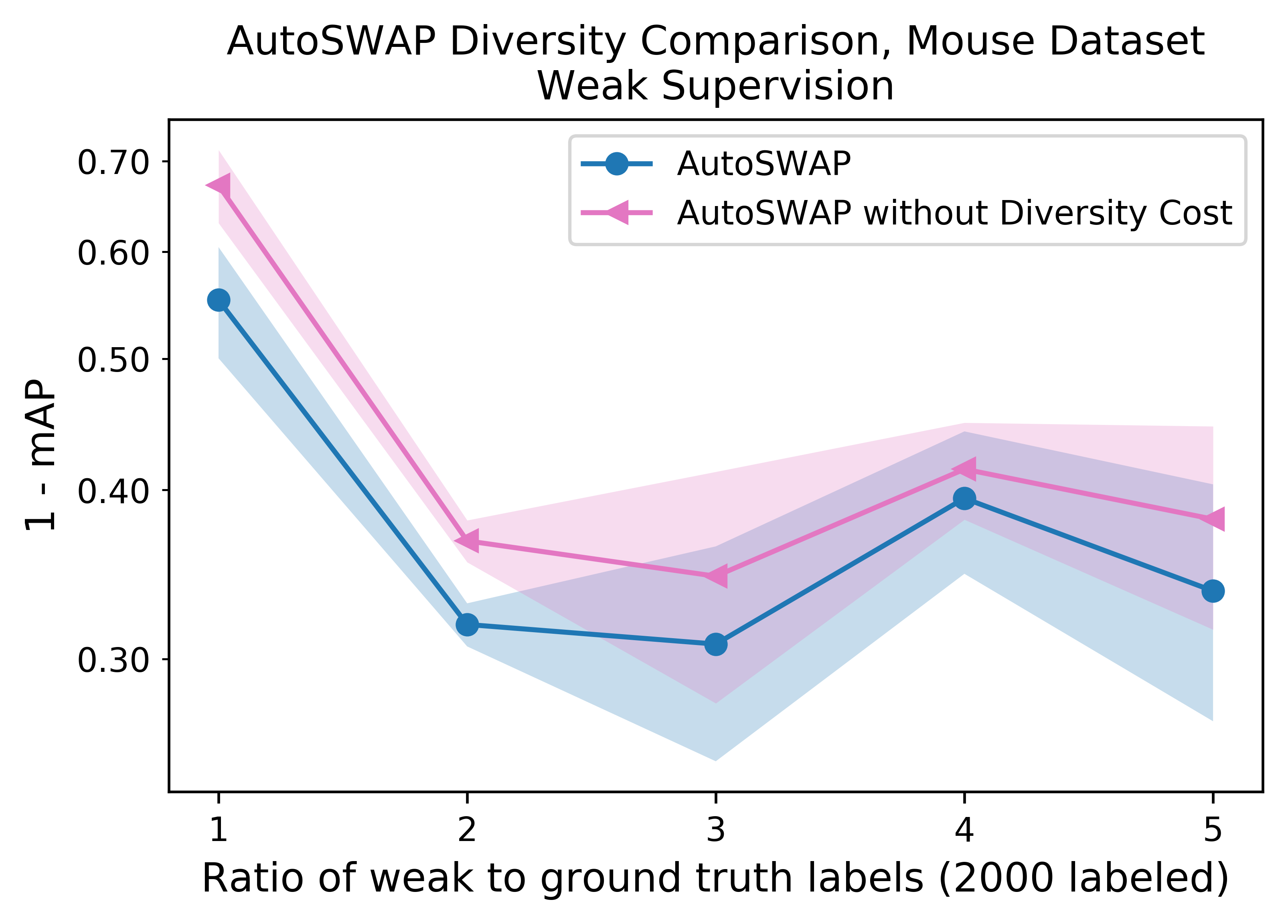
Figure 6: Diversity Cost Utility Comparison. Synthesizing diverse sets of programs instead of purely $\epsilon$-optimal sets improves AutoSWAP, showing the utility of the structural diversity cost.

AutoSWAP Diversity Cost. The diversity cost is an important part of AutoSWAP. As can be seen in Figure 6, synthesizing purely optimal programs w.r.t. Equation 1 results in worse performance than synthesizing diverse sets of programs. This mirrors the observations in [33], where using diverse sets of decision trees improves performance.

Interpretability of Labeling Functions. An important part of behavior analysis is being able to interpret learned models. Neural networks and LSTMs are by nature not interpretable. Decision trees offer some degree of interpretability, but are limited to branched if-then-else statements. With AutoSWAP, complex yet interpretable programs can be learned by using interpretable structures in the DSL (Figures 3, 7, Supplementary Materials).

Effect on Rare Behaviors. Rare behaviors can be difficult to analyze, as even with large datasets very little data exists. Our fly domain results show that AutoSWAP greatly improves data efficiency for rare behaviors, as 5 of the 6 behaviors we study occur in $<5\%$ of the frames. We note the copulation task (which is not rare) does not bias our Fly domain data efficiency comparison as all tested methods achieve near-perfect performance on it.

⬇

Fly Domain:

(Lunge) Map(Add(Multiply(Speed, WingRatio), Positional))

(Tussle) Map(SimpleITE(Angular, Speed, WingDistance))))

Mouse Domain:

Map(Fold(SimpleITE(DistanceM1, AngleM1, SpeedM1)))

Map(SimpleITE(PositionalM2, SpeedM1, DistanceM1))

Basketball Domain:

Fold(Add(PlAccel(), Add(PlPos(), PlVel())))

Fold(SimpleITE(BVel(), PlVel(), PlPos()))

Figure 7: Example AutoSWAP task-level LFs (architectures only). LFs are composed of domain-level LFs and structural relations from the DSL. For example, the “Fly Lunge LF” labels whether a fly is lunging using the fly’s speed, wing ratio, and positional domain-level LFs. More detailed descriptions of AutoSWAP LFs can be found in the Supplementary Materials.

6 Discussion and Conclusion

We propose AutoSWAP, a framework that uses program synthesis to automatically synthesize diverse LFs. Our results demonstrate the effectiveness of our framework in both active learning and weak supervision settings and across three behavior analysis settings. We find that with existing domain-level LFs [14, 24] and a simple DSL, AutoSWAP can synthesize highly data efficient task-level LFs with minimal amounts of labeled data, thus reducing annotation requirements for domain experts.

Additionally, we introduce a novel structural diversity cost and admissible heuristic for synthesized programs, which allows AutoSWAP to scalably synthesize diverse LFs with informed search algorithms. This further improves the performance of our framework in behavior analysis settings, all without requiring domain experts to repeatedly hand-craft task-level LFs. Overall, AutoSWAP effectively integrates weak supervision with behavior analysis, and greatly reduces domain expert effort through automatically synthesizing task-level LFs from domain-level knowledge.

Limitations. While our DSL and LFs are at the domain-level, our method requires task-level information in the form of a small labeled dataset to synthesize LFs. Additionally, the LFs provided by domain experts should be informative of behavior (although we do show that current behavioral features [14, 24] studied by domain experts are sufficient for this task). Extensions to automate other aspects of our framework while taking into account domain expert knowledge, such as library learning [11] or integrating perception [32], may further reduce expert effort. However, we note that our current framework already leads to significant reductions in data requirements.

Societal Impact. Automatically generating interpretable LFs to reduce expert effort can help behavior analysis across domains, such as in neuroscience, ethology, sports analytics, and autonomous vehicles, among others. Our framework leverages inductive biases in the DSL to produce interpretable programs; however, since humans create the DSL, interpret programs, and annotate data, users should be aware of potential human-encoded biases in these steps. Additional care is especially needed in human behavior domains, such as with informed consent of participants and responsible handling of data.

7 Acknowledgements

We thank Adith Swaminathan at Microsoft Research and Pietro Perona at Caltech for their feedback and discussions regarding this work. We also thank Microsoft Research for compute resources. This work is partially supported by NSF Award #1918839 (YY) and NSERC Award #PGSD3-532647-2019 (JJS).

References

- [1] David J Anderson and Pietro Perona. Toward a science of computational ethology. Neuron, 84(1):18–31, 2014.
- [2] Jenna Wiens Armand McQueen and John Guttag. Automatically recognizing on-ball screens. In MIT Sloan Sports Analytics Conference, 2014.
- [3] Gordon J Berman, Daniel M Choi, William Bialek, and Joshua W Shaevitz. Mapping the stereotyped behaviour of freely moving fruit flies. Journal of The Royal Society Interface, 11(99):20140672, 2014.
- [4] Samantha Biegel, Rafah El-Khatib, Luiz Otavio Vilas Boas Oliveira, Max Baak, and Nanne Aben. Active weasul: Improving weak supervision with active learning. arXiv preprint arXiv:2104.14847, 2021.
- [5] Benedikt Boecking, Willie Neiswanger, Eric Xing, and Artur Dubrawski. Interactive weak supervision: Learning useful heuristics for data labeling. In International Conference on Learning Representations, 2021.
- [6] Adam J Calhoun, Jonathan W Pillow, and Mala Murthy. Unsupervised identification of the internal states that shape natural behavior. Nature neuroscience, 22(12):2040–2049, 2019.
- [7] Ming-Fang Chang, John Lambert, Patsorn Sangkloy, Jagjeet Singh, Slawomir Bak, Andrew Hartnett, De Wang, Peter Carr, Simon Lucey, Deva Ramanan, et al. Argoverse: 3d tracking and forecasting with rich maps. In Proceedings of the IEEE Conference on Computer Vision and Pattern Recognition, pages 8748–8757, 2019.
- [8] Qiaochu Chen, Aaron Lamoreaux, Xinyu Wang, Greg Durrett, Osbert Bastani, and Isil Dillig. Web question answering with neurosymbolic program synthesis. In Proceedings of the 42nd ACM SIGPLAN International Conference on Programming Language Design and Implementation, pages 328–343, 2021.
- [9] James Colyar and John Halkias. Us highway 101 dataset. Federal Highway Administration (FHWA), Tech. Rep. FHWA-HRT-07-030, 2007.
- [10] Jared A. Dunnmon, Alexander J. Ratner, Khaled Saab, Nishith Khandwala, Matthew Markert, Hersh Sagreiya, Roger Goldman, Christopher Lee-Messer, Matthew P. Lungren, Daniel L. Rubin, and Christopher Ré. Cross-modal data programming enables rapid medical machine learning. Patterns, 1(2):100019, 2020.
- [11] Kevin Ellis, Lucas Morales, Mathias Sablé-Meyer, Armando Solar-Lezama, and Josh Tenenbaum. Learning libraries of subroutines for neurally–guided bayesian program induction. In S. Bengio, H. Wallach, H. Larochelle, K. Grauman, N. Cesa-Bianchi, and R. Garnett, editors, Advances in Neural Information Processing Systems, volume 31. Curran Associates, Inc., 2018.
- [12] Kevin Ellis, Daniel Ritchie, Armando Solar-Lezama, and Josh Tenenbaum. Learning to infer graphics programs from hand-drawn images. In S. Bengio, H. Wallach, H. Larochelle, K. Grauman, N. Cesa-Bianchi, and R. Garnett, editors, Advances in Neural Information Processing Systems, volume 31. Curran Associates, Inc., 2018.
- [13] Kevin Ellis, Armando Solar-Lezama, and Josh Tenenbaum. Unsupervised learning by program synthesis. 2015.
- [14] Eyrun Eyjolfsdottir, Steve Branson, Xavier P Burgos-Artizzu, Eric D Hoopfer, Jonathan Schor, David J Anderson, and Pietro Perona. Detecting social actions of fruit flies. In European Conference on Computer Vision, pages 772–787. Springer, 2014.
- [15] John K Feser, Swarat Chaudhuri, and Isil Dillig. Synthesizing data structure transformations from input-output examples. ACM SIGPLAN Notices, 50(6):229–239, 2015.
- [16] Larry R. Harris. The heuristic search under conditions of error. Artif. Intell., 5:217–234, 1974.
- [17] Giannis Karamanolakis, Subhabrata (Subho) Mukherjee, Guoqing Zheng, and Ahmed H. Awadallah. Self-training with weak supervision. In NAACL 2021. NAACL 2021, May 2021.
- [18] David Lewis, Jason Catlett, W. Cohen, and Haym Hirsh. Heterogeneous uncertainty sampling for supervised learning. 12 1996.
- [19] Kevin Luxem, Falko Fuhrmann, Johannes Kürsch, Stefan Remy, and Pavol Bauer. Identifying behavioral structure from deep variational embeddings of animal motion. bioRxiv, 2020.
- [20] Mona Nashaat, Aindrila Ghosh, James Miller, Shaikh Quader, Chad Marston, and Jean-Francois Puget. Hybridization of active learning and data programming for labeling large industrial datasets. In 2018 IEEE International Conference on Big Data (Big Data), pages 46–55. IEEE, 2018.
- [21] Emilio Parisotto, Abdel-rahman Mohamed, Rishabh Singh, Lihong Li, Dengyong Zhou, and Pushmeet Kohli. Neuro-symbolic program synthesis. arXiv preprint arXiv:1611.01855, 2016.
- [22] Alexander Ratner, Braden Hancock, Jared Dunnmon, Frederic Sala, Shreyash Pandey, and Christopher Ré. Training complex models with multi-task weak supervision. Proceedings of the AAAI Conference on Artificial Intelligence, 33(01):4763–4771, Jul. 2019.
- [23] Alexander J Ratner, Christopher M De Sa, Sen Wu, Daniel Selsam, and Christopher Ré. Data programming: Creating large training sets, quickly. Advances in neural information processing systems, 29:3567–3575, 2016.
- [24] Cristina Segalin, Jalani Williams, Tomomi Karigo, May Hui, Moriel Zelikowsky, Jennifer J. Sun, Pietro Perona, David J. Anderson, and Ann Kennedy. The mouse action recognition system (mars): a software pipeline for automated analysis of social behaviors in mice. bioRxiv https://doi.org/10.1101/2020.07.26.222299, 2020.
- [25] Ameesh Shah, Eric Zhan, Jennifer J Sun, Abhinav Verma, Yisong Yue, and Swarat Chaudhuri. Learning differentiable programs with admissible neural heuristics. In Neural Information Processing Systems, 2020.
- [26] Armando Solar-Lezama, Liviu Tancau, Rastislav Bodik, Sanjit Seshia, and Vijay Saraswat. Combinatorial sketching for finite programs. In Proceedings of the 12th international conference on Architectural support for programming languages and operating systems, pages 404–415, 2006.
- [27] Jennifer J. Sun, Tomomi Karigo, Dipam Chakraborty, Sharada Mohanty, Benjamin Wild, Quan Sun, Chen Chen, David Anderson, Pietro Perona, Yisong Yue, and Ann Kennedy. The multi-agent behavior dataset: Mouse dyadic social interactions. In Thirty-fifth Conference on Neural Information Processing Systems Datasets and Benchmarks Track (Round 1), 2021.
- [28] Jennifer J Sun, Ann Kennedy, Eric Zhan, David J Anderson, Yisong Yue, and Pietro Perona. Task programming: Learning data efficient behavior representations. In Conference on Computer Vision and Pattern Recognition, 2021.
- [29] Tao Sun and Zhi-Hua Zhou. Structural diversity for decision tree ensemble learning. Frontiers of Computer Science, 12, 02 2018.
- [30] Karl Tuyls, Shayegan Omidshafiei, Paul Muller, Zhe Wang, Jerome Connor, Daniel Hennes, Ian Graham, William Spearman, Tim Waskett, Dafydd Steel, et al. Game plan: What ai can do for football, and what football can do for ai. Journal of Artificial Intelligence Research, 71:41–88, 2021.
- [31] Lazar Valkov, Dipak Chaudhari, Akash Srivastava, Charles Sutton, and Swarat Chaudhuri. Houdini: Lifelong learning as program synthesis. In Advances in neural information processing systems, 2018.
- [32] Lazar Valkov, Dipak Chaudhari, Akash Srivastava, Charles Sutton, and Swarat Chaudhuri. Houdini: Lifelong learning as program synthesis. In S. Bengio, H. Wallach, H. Larochelle, K. Grauman, N. Cesa-Bianchi, and R. Garnett, editors, Advances in Neural Information Processing Systems, volume 31. Curran Associates, Inc., 2018.
- [33] Paroma Varma and Christopher Ré. Snuba: Automating weak supervision to label training data. In Proceedings of the VLDB Endowment. International Conference on Very Large Data Bases, volume 12, page 223. NIH Public Access, 2018.
- [34] Abhinav Verma, Vijayaraghavan Murali, Rishabh Singh, Pushmeet Kohli, and Swarat Chaudhuri. Programmatically interpretable reinforcement learning. In International Conference on Machine Learning, pages 5045–5054. PMLR, 2018.
- [35] Qizhe Xie, Minh-Thang Luong, Eduard Hovy, and Quoc V. Le. Self-training with noisy student improves imagenet classification, 2020.
- [36] Yisong Yue, Patrick Lucey, Peter Carr, Alina Bialkowski, and Iain Matthews. Learning fine-grained spatial models for dynamic sports play prediction. In 2014 IEEE international conference on data mining, pages 670–679. IEEE, 2014.
- [37] Eric Zhan, Stephan Zheng, Yisong Yue, Long Sha, and Patrick Lucey. Generating multi-agent trajectories using programmatic weak supervision. In International Conference on Learning Representations, 2019.
- [38] Kaizhong Zhang and Dennis Shasha. Simple fast algorithms for the editing distance between trees and related problems. SIAM J. Comput., 18:1245–1262, 12 1989.