SamplingAug: On the Importance of Patch Sampling Augmentation for Single Image Super-Resolution

Abstract

With the development of Deep Neural Networks (DNNs), plenty of methods based on DNNs have been proposed for Single Image Super-Resolution (SISR). However, existing methods mostly train the DNNs on uniformly sampled LR-HR patch pairs, which makes them fail to fully exploit informative patches within the image. In this paper, we present a simple yet effective data augmentation method. We first devise a heuristic metric to evaluate the informative importance of each patch pair. In order to reduce the computational cost for all patch pairs, we further propose to optimize the calculation of our metric by integral image, achieving about two orders of magnitude speedup. The training patch pairs are sampled according to their informative importance with our method. Extensive experiments show our sampling augmentation can consistently improve the convergence and boost the performance of various SISR architectures, including EDSR, RCAN, RDN, SRCNN and ESPCN across different scaling factors ($\times 2$, $\times 3$, $\times 4$). Code is available at https://github.com/littlepure2333/SamplingAug.

1 Introduction

Single Image Super-Resolution (SISR) is a long-standing problem in computer vision. With the rapid development of Deep Neural Networks (DNNs) over the past few years, plenty of SISR methods based on DNNs are proposed. These methods mainly focus on network design [Shi et al.(2016)Shi, Caballero, Huszár, Totz, Aitken, Bishop, Rueckert, and Wang, Dong et al.(2014)Dong, Loy, He, and Tang, Kim et al.(2016)Kim, Kwon Lee, and Mu Lee, Zhang et al.(2018a)Zhang, Li, Li, Wang, Zhong, and Fu, Lim et al.(2017)Lim, Son, Kim, Nah, and Mu Lee], real-world SR [Cai et al.(2019)Cai, Zeng, Yong, Cao, and Zhang, Xu et al.(2019)Xu, Ma, and Sun], zero-shot learning [Shocher et al.(2018)Shocher, Cohen, and Irani, Shaham et al.(2019)Shaham, Dekel, and Michaeli], meta learning [Park et al.(2020)Park, Yoo, Cho, Kim, and Kim, Soh et al.(2020)Soh, Cho, and Cho], network efficiency [Hui et al.(2018)Hui, Wang, and Gao, Xin et al.(2020)Xin, Wang, Jiang, Li, Huang, and Gao], etc. However, as one of the most practical techniques, data augmentation has been rarely studied for SISR.

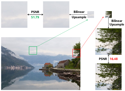
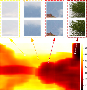
a) Illustration of informative importance	b) Illustration of patch sampling

Figure 1: a) Illustration of informative importance. There are both easy and hard patches within the image. Flat regions are easy to restore even with bilinear interpolation. However, patches with complicated texture are hard to restore. b) Illustration of patch sampling. According to the informative map, our method can sort all possible patches and take the informative patches for training.

Recently, [Yoo et al.(2020)Yoo, Ahn, and Sohn] provides a comprehensive analysis of applying data augmentation methods used in high-level vision tasks to SISR. Based on the analysis, they further propose a new augmentation method named CutBlur, which can reduce unrealistic distortions. Apart from CutBlur [Yoo et al.(2020)Yoo, Ahn, and Sohn], former works mostly rely on simple geometric manipulations like rotation and flipping to the best of our knowledge. The motivation of CutBlur is to regularize a model to learn not only “how” but also “where” to apply the super-resolution to a given image. This indicates that spatial information is also essential for SISR data augmentation in addition to simple geometric manipulations.

Although CutBlur can achieve consistent improvements, it still follows the methodology of Mixup [Zhang et al.(2017)Zhang, Cisse, Dauphin, and Lopez-Paz] and CutMix [Yun et al.(2019)Yun, Han, Oh, Chun, Choe, and Yoo], which are designed for high-level vision tasks. Since existing SISR methods mostly train the DNNs on sampled LR-HR patch pairs, we study the data augmentation problem from the perspective of patch sampling in this paper. Recent work on demosaicing and denoising [Sun et al.(2020)Sun, Chen, Slabaugh, and Torr] also investigates the problem of patch sampling. They train an additional PatchNet to select more informative patch samples for training and significantly enhance the network performance. In contrast to training an additional DNN, we propose a heuristic metric to evaluate the informative importance of each patch pair. Our metric is motivated by the fact that DNN can be treated as a highly non-linear function learned from data. Therefore, patches that can be super-resolved by linear function should be less informative for training the DNN. Inspired by this, we define the metric as the PSNR between linear SR and HR for each patch pair.

However, directly calculating the metric for all patch pairs of an image is computationally complicated. We further propose to accelerate the calculation of our metric by integral image. Instead of using sliding windows, we first obtain the integral images of linear SR and HR separately, and then the integral images are used to deliver the metric for individual patch pair. By this way, we can significantly reduce the computational cost and achieve about two-orders of magnitude speedup.

After obtaining the informative importance of each patch pair, we need to sample a portion of patches for DNN training. We consider three sampling strategies. The first is simply selecting the $p\%$ most informative patches according to the metric. The second is applying Non-Maximum Suppression (NMS) [Girshick(2015)] to sampling the patches. The third is adopting Throwing-Dart (TD) sampling strategy [Gharbi et al.(2016)Gharbi, Chaurasia, Paris, and Durand] based on the metric. The latter two strategies can result in non-overlapped sampling across the image. All these three strategies can achieve consistent performance improvement on various popular architectures [Lim et al.(2017)Lim, Son, Kim, Nah, and Mu Lee, Zhang et al.(2018a)Zhang, Li, Li, Wang, Zhong, and Fu, Dong et al.(2014)Dong, Loy, He, and Tang, Shi et al.(2016)Shi, Caballero, Huszár, Totz, Aitken, Bishop, Rueckert, and Wang]. Besides, to our surprise, simply selecting the $p\%$ most informative patches achieves even slightly better results compared with NMS and TD, indicating that less informative samples might not contribute to the performance of SISR. We hope our paper can inspire future work on data augmentation for SISR.

Our contributions can be concluded as follows:

• We propose a simple heuristic metric, which can effectively measure the informative importance of each LR-HR patch pair for SISR training.

• We present an efficient method for metric calculation, which significantly reduces the computational cost.

• We conduct extensive experiments with various SISR architectures, different scaling factors, and sampling strategies to demonstrate the benefit of our work.

2 Related Work

DNN-based Image Super-Resolution Since the pioneering work SRCNN [Dong et al.(2014)Dong, Loy, He, and Tang], many DNN-based methods have been proposed. VDSR [Kim et al.(2016)Kim, Kwon Lee, and Mu Lee] adopts a very deep DNN to learn the image residual. EDSR [Lim et al.(2017)Lim, Son, Kim, Nah, and Mu Lee] analyzes the DNN layers and removes some redundant layers from SRResNet [Ledig et al.(2017)Ledig, Theis, Huszár, Caballero, Cunningham, Acosta, Aitken, Tejani, Totz, Wang, et al.]. RDN [Zhang et al.(2018b)Zhang, Tian, Kong, Zhong, and Fu] introduces dense connections to fully utilize the information of preceding layers. RCAN [Zhang et al.(2018a)Zhang, Li, Li, Wang, Zhong, and Fu] explores the attentions mechanism for SR. FSRCNN [Dong et al.(2016)Dong, Loy, and Tang] and ESPCN [Shi et al.(2016)Shi, Caballero, Huszár, Totz, Aitken, Bishop, Rueckert, and Wang] propose to use LR image as input and upscale the feature map at the end of DNNs. LAPAR [Li et al.(2020)Li, Zhou, Qi, Jiang, Lu, and Jia] presents a method based on linearly-assembled pixel-adaptive regression network. ClassSR [Kong et al.(2021)Kong, Zhao, Qiao, and Dong] accelerates SR networks on large images (2K-8K) by combining classification and SR in a unified framework. Although plenty of DNN-based methods are proposed, as one of the most practical ways to improve model performance, data augmentation has been rarely studied for SISR.

Patch Sampling To the best of our knowledge, DNNs of SR are mostly trained on uniformly sampled LR-HR patch pairs and tested on images. However, there are hard and simple areas within a single image. KPN [Bako et al.(2017)Bako, Vogels, McWilliams, Meyer, Novák, Harvill, Sen, Derose, and Rousselle] uses a sampling strategy named Throwing Dart (TD), according to the importance map delivered from additional rendered buffers. PatchNet [Sun et al.(2020)Sun, Chen, Slabaugh, and Torr] recently learns to select the most useful patches from an image to construct a training set instead of random selection. They significantly boost the performance of demosaicing and denoising. Our work also tries to select the informative patch pairs for DNN training. In contrast to training a network, we propose an efficient heuristic metric to evaluate the informative importance of LR-HR patch pair.

3 Method

In this part, we first present the effective metric that evaluates the informative importance of patch pair in Section 3.1. Then we introduce an acceleration solution based on integral image in Section 3.2. Finally, we briefly describe three sampling strategies in Section 3.3.

3.1 Informative Importance Metric

Existing SISR methods [Lim et al.(2017)Lim, Son, Kim, Nah, and Mu Lee, Zhang et al.(2018a)Zhang, Li, Li, Wang, Zhong, and Fu] mostly train the DNNs with sampled LR-HR patch pairs rather than the whole images due to the memory limitation. The patches are usually uniformly sampled to construct a training batch. As shown in Fig 1 a), we observe that there are easy patches and hard patches even within a single image. For example, flat regions are easy to restore even with bilinear interpolation, while regions with complicated textures are hard to restore. Furthermore, the recent success of DNN is largely due to its non-linear capability learned from database. Inspired by this observation, we propose to explore the informative importance of each patch pair by defining a heuristic metric. To be more specific, let $x^{LR}$ and $x^{HR}$ be the LR and HR patches. The patch size of $x^{HR}$ is $k\times k$ and the scaling factor is $s$. We first upscale $x^{LR}$ to the SR patch ${x^{\widetilde{SR}}}$ with bilinear interpolation. Then we define the heuristic metric as the PSNR between ${x^{\widetilde{SR}}}$ and $x^{HR}$. This process can be formulated as follow:

$$MSE=\frac{1}{k^{2}}\sum_{i=0}^{k-1}\sum_{j=0}^{k-1}||x_{i,j}^{\widetilde{SR}}-x_{i,j}^{HR}||_{2}^{2}$$ (1)

$$PSNR=10*log_{10}(\frac{MAX_{x}^{2}}{MSE})$$ (2)

where $MAX_{x}$ is the maximum possible pixel value of the image and is set to 255 for 8-bit format. Higher PSNR between ${x^{\widetilde{SR}}}$ and $x^{HR}$ indicates that this patch is less informative for DNN training since the linear restoration can already achieve pleasing restoration results. As illustrated by Fig 1 b), for every image in the database, we can sort all the possible patch pairs by calculating the PSNR between ${x^{\widetilde{SR}}}$ and $x^{HR}$, and take the $p\%$ most informative patches for training.

3.2 Integral Image Acceleration

As described previously, our method needs to calculate the PSNR between all possible patch pairs. Assume there are $N$ images under resolution $H\times W$, the computational complexity of sliding windows is $O(NHW)$. Although it can be accelerated by GPU parallel computing, our primary GPU implementation still takes about 10 seconds to process an image in 2K resolution.

To overcome this, we optimize the calculation process using integral image [Crow(1984)]. Specifically, instead of bilinearly interpolating the local patch, we upscale the LR image ${X^{LR}}$ to ${X^{\widetilde{SR}}}$. For a patch pair (top left pixel location is $(u,v)$), we can represent the MSE in Eq. 1 as:

$$MSE=\frac{1}{{{k^{2}}}}\sum\limits_{i=0}^{k-1}{\sum\limits_{j=0}^{k-1}{\left\|{X_{(u+i,j+v)}^{\widetilde{SR}}-X_{(u+i,j+v)}^{HR}}\right\|_{2}^{2}}}$$ (3)

The above equation can be expanded and summarized into:

$$MSE=\frac{1}{{{k^{2}}}}\sum\limits_{i=0}^{k-1}{\sum\limits_{j=0}^{k-1}{X_{(u+i,j+v)}^{HR}X_{(u+i,j+v)}^{HR}}}+\frac{1}{{{k^{2}}}}\sum\limits_{i=0}^{k-1}{\sum\limits_{j=0}^{k-1}{X_{(u+i,j+v)}^{\widetilde{SR}}X_{(u+i,j+v)}^{\widetilde{SR}}}}$$ (4)

$$-2\frac{1}{{{k^{2}}}}\sum\limits_{i=0}^{k-1}{\sum\limits_{j=0}^{k-1}{X_{(u+i,j+v)}^{HR}X_{(u+i,j+v)}^{\widetilde{SR}}}}$$

For each term in Eq. 4, we observe it can be significantly accelerated by integral image. We denote the integral image as $\gamma(*)$ and reformulate the first term as:

$$\sum\limits_{i=0}^{k-1}{\sum\limits_{j=0}^{k-1}{X_{(u+i,j+v)}^{HR}X_{(u+i,j+v)}^{HR}}}=\gamma{({X^{HR}}\odot{X^{HR}})_{\overline{u},\overline{v}}}+\gamma{({X^{HR}}\odot{X^{HR}})_{u,v}}$$ (5)

$$-\gamma{({X^{HR}}\odot{X^{HR}})_{\overline{u},v}}-\gamma{({X^{HR}}\odot{X^{HR}})_{u,\overline{v}}}$$

where $\odot$ denotes the element-wise multiplication, $\overline{u}=u+k-1$ and $\overline{v}=v+k-1$ are the bottom right pixel locations. We omit the constant $\frac{1}{{{k^{2}}}}$ for simplicity. The second and third terms of Eq. 4 can be reformulated similarly. Using integral image [Crow(1984)] avoids traversing all patch pairs, greatly reducing the computational complexity. The proposed algorithm takes 0.1 second to process a 2K image, achieving about two orders of magnitude speedup compared with primary GPU implementation (10 seconds).

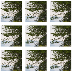
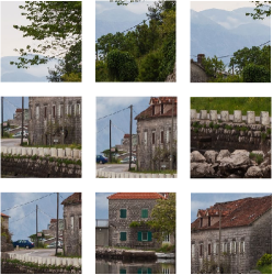
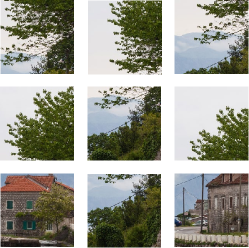
a) GS	b) TDS	c) NMSS

Figure 2: Example of selected patches with different sampling strategies. Greedy sampling will select overlapped patches, while Throwing Dart sampling and NMS sampling result in non-overlapped patches.

3.3 Different Sampling Strategies

Greedy Sampling (GS) Based on the informative importance map, we can use greedy sampling strategy, which directly gathers the $p\%$ most informative patches. As shown in Fig. 2, greedy sampling will result in heavily overlapped patches. This sampling strategy is our default strategy used in the paper. To further study the benefit of non-overlapped sampling, we also design two variant strategies.

Throwing Dart Sampling (TDS) Throwing-Dart Sampling [Bako et al.(2017)Bako, Vogels, McWilliams, Meyer, Novák, Harvill, Sen, Derose, and Rousselle] can automatically choose non-overlapped patches. This strategy first generates non-overlapped candidates by employing throwing darts. The patch candidates are pruned according to the importance map to deliver $p\%$ patches for training. [Bako et al.(2017)Bako, Vogels, McWilliams, Meyer, Novák, Harvill, Sen, Derose, and Rousselle] adopts the rendered normal and color images to obtain the importance map. In this work, we use the proposed informative metric to obtain the importance map. As illustrated by Fig. 2, TDS can construct non-overlapped patches for DNN training.

Non-maximum Suppression Sampling (NMSS) Non-maximum suppression [Girshick(2015)] is a technique widely used in object detection. Inspired by NMS, we first select the most informative patch and mask out all overlapped patches with IoU higher than a threshold. Then, we select the next most informative patch from the remaining candidate patches. This process is repeated to construct $p\%$ patches as the training samples. In this manner, NMSS will select non-overlapped patches for training. We show the examples of selected patches in Fig. 2.

4 Experiment

4.1 Experimental setup

We use DIV2K dataset [Agustsson and Timofte(2017)] for training, which consists of 1000 high-resolution images in 2K resolution. The low-resolution images are generated by bicubic downsampling with scaling factors of $\times 2$, $\times 3$ and $\times 4$. Following former works, we use 800 images for training and 10 images for validation. We also report results on four standard benchmark datasets including Set5, Set14, B100 and Urban100. Peak Signal-to-Noise Ratio (PSNR) and Structural Similarity (SSIM) are adopted as the evaluation metrics to measure SR performance. We ignore image borders and calculate the PSNR and SSIM in the luminance channels.

4.2 Implementation Details

To verify the effectiveness and generalization of our method, we use 5 popular SISR architectures as baselines including SRCNN, ESPCN, EDSR, RCAN and RDN. All the experiments are conducted with PyTorch framework on NVIDIA 2080Ti GPUs. The patch size is set to $192\times 192$ during training unless mentioned otherwise. We use Adam optimizer with $\beta_{1}=0.9$ and $\beta_{2}=0.999$. All models are trained 300 epochs from scratch using the above experimental setups. By integral Image Acceleration, processing whole DIV2K dataset takes additional 3 minutes for greedy sampling, 5 minutes for NMS sampling and 1 minutes for throwing darts sampling. The additional cost of our method is almost negligible.

4.3 Results on Various SISR Architectures

4.3.1 Quantitative Results

In Tab. 1, we show a comprehensive quantitative comparison with various baseline models under different scaling factors. As can be seen, the proposed method consistently boosts the PSNR performance across various popular baseline architectures, scaling factors and benchmark datasets by adequate margins. We also provide the SSIM results in the supplementary material. Surprisingly, for the lightweight models, our method brings significant benefits. For example, on Set5 and scaling factor $\times 2$, SRCNN and ESPCN obtain huge margins of 1.40 dB and 2.26 dB respectively. All the results show that our method can yield a consistent and significant performance boost.

Networks	scale	Set5	Set14	B100	Urban100
	x2	34.94 (+1.40)	31.62 (+1.11)	30.47 (+0.87)	27.79 (+0.90)
SRCNN	x3	31.37 (+0.47)	28.60 (+0.40)	27.77 (+0.26)	25.06 (+0.28)
	x4	29.33 (+0.35)	26.91 (+0.30)	26.42 (+0.16)	23.63 (+0.18)
	x2	34.05 (+2.26)	31.14 (+1.91)	30.36 (+1.23)	27.64 (+1.30)
ESPCN	x3	30.36 (+1.36)	27.93 (+1.07)	27.50 (+0.70)	24.76 (+0.75)
	x4	28.20 (+1.26)	26.13 (+0.89)	26.10 (+0.65)	23.28 (+0.68)
	x2	37.27 (+0.40)	33.38 (+0.41)	31.68 (+0.27)	30.46 (+0.86)
EDSR	x3	33.02 (+0.33)	29.86 (+0.25)	28.49 (+0.13)	26.44 (+0.35)
	x4	30.66 (+0.33)	27.93 (+0.30)	26.94 (+0.11)	24.58 (+0.27)
	x2	36.85 (+0.15)	32.97 (+0.09)	31.40 (+0.06)	29.62 (+0.21)
RCAN	x3	32.71 (+0.58)	29.61 (+0.39)	28.34 (+0.22)	26.16 (+0.50)
	x4	30.35 (+0.48)	27.68 (+0.42)	26.83 (+0.18)	24.37 (+0.36)
	x2	37.20 (+0.07)	33.25 (+0.17)	31.65 (+0.11)	30.22 (+0.38)
RDN	x3	33.15 (+0.34)	29.87 (+0.18)	28.57 (+0.15)	26.51 (+0.36)
	x4	30.70 (+0.34)	28.00 (+0.33)	26.99 (+0.14)	24.63 (+0.31)

Table 1: Quantitative Results (PSNR) on Benchmarks. We omit the results of baselines for simplicity, and only report our results and the gain margins. SSIM results are reported in supplemental material.

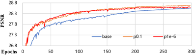
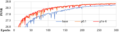
a) EDSR	b) RDN

Figure 3: Convergence analysis of our method. We show the training process of EDSR and RDN in scaling factor $\times 4$. Our results of $p=0.1$ and $p=1e-6$ are shown in this figure for illustration. As can be seen, our method can consistently improve the convergence and performance of SR networks.

4.3.2 Convergence Results

Fig. 3 shows the convergence comparison between the baselines and our method. It can be observed that our method can also help the training process converge faster. In particular, the results of our method at 150 epochs already achieve the performance of baselines at 300 epochs. Fig. 3 also shows our results of different sampling portion $p\%$. We observe that selecting fewer patches ($p=1e-6$) increases the convergence speed at the early stage, while more informative patches ($p=0.1$) can achieve better results after convergence. This enables our method to achieve a flexible balance between training time and performance.

4.3.3 Qualitative Results

Fig. 4 shows the qualitative results of our method against the baselines. All the SR networks benefit from our method and obtain visually better results. We provide more qualitative results in the supplementary materials.

4.4 Ablation Study

4.4.1 Impact of patch size.

Since our method measures the informative importance for each LR-HR patch pair, it is essential to study the impact of patch size to evaluate our method. We show the results of our method with different patch sizes in Tab. 3. Our method obtains consistent and significant gain margins, and especially effective for smaller patch size.

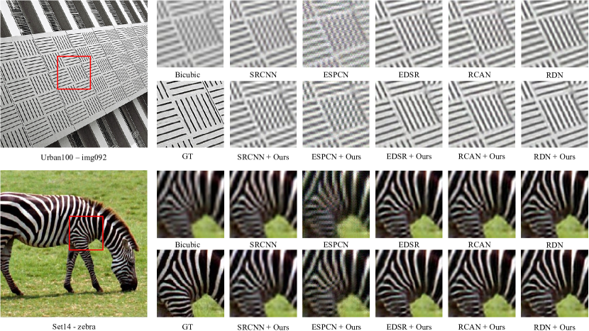
Figure 4: Qualitative comparison between our method and baselines (x4 SR). More results can be found in the supplementary material.

patch size	baseline	ours
32	27.71	28.27 (+0.56)
64	28.10	28.48 (+0.38)
128	28.16	28.50 (+0.34)
192	28.55	28.69 (+0.14)
256	28.58	28.69 (+0.11)
384	28.90	28.95 (+0.05)

Table 2: Ablation study on different patch size. The PSNR results of EDSR are reported in DIV2K dataset at x4 scale.

	ESPCN	EDSR
baseline	29.24	34.56
0.5	31.04 (+1.80)	34.67 (+0.11)
0.3	31.34 (+2.10)	34.68 (+0.12)
0.1	31.52 (+2.28)	34.68 (+0.12)
1e-2	31.72 (+2.48)	34.64 (+0.08)
1e-3	31.78 (+2.54)	34.62 (+0.06)
1e-4	31.77 (+2.53)	34.61 (+0.05)
1e-5	31.78 (+2.54)	34.60 (+0.04)
1e-6	31.78 (+2.54)	34.62 (+0.06)

Table 3: Ablation study of varying portion. The PSNR results are reported in DIV2K dataset at x2 scale.

4.4.2 Impact of sampled portion.

We conduct extensive experiments to explore the SR performance under different portions of informative data. The results in Tab. 3 show that networks with strong capacity (EDSR, RCAN and RDN) obtain the best performance when $p$ is set to 0.1. We think 10% most informative patch pairs are the optimal choice for these networks, since more data will introduce “noisy” samples and less data cannot meet the capacity of these networks. While for lightweight networks like SRCNN and ESPCN, they achieve the best performance when $p$ is set to $1e^{-5}$, this is perhaps because their capacity is less strong and a few of most informative samples already meet their capacity. Therefore, stronger capacity models can utilize more informative data to achieve the best performance. Nevertheless, even when $p$ is extremely small, the proposed method can still boost the performance compared with baselines. To our surprise, just only selecting one most informative patch per image ($p=1e^{-6}$) can already overpass the results of uniformly sampling all patches, validating the effectiveness of our method.

4.4.3 Do other metrics help?

Apart from our metric, we also try other heuristic metrics to measure the informative importance of local patch. We use the Standard Deviation (STD) of the patch since STD can kind of model the texture information. We also try to use edge detection operators (Sobel, Canny and Laplacian) to measure the informative importance. Tab. 5 shows the results of these metrics, where $std0$ means the STD of all channels (RGB), $std1$ means the mean of each channel’s STD (RGB), and $std2$ means the STD of y channel (YCbCr). As can be seen, our method achieves better results compared with these metrics, demonstrating the advantages of our metric. All the results show the effectiveness of our metric to measure the informative importance of LR-HR patch pair.

4.4.4 Do sampling strategies matter?

As mentioned above, we simply adopt the Greedy Sampling (GS) strategy, which will sample heavily overlapped patches for training. In order to study the benefit of non-overlapped sampling, we compare GS with NMS [Girshick(2015)] sampling and Throwing-Dart sampling [Bako et al.(2017)Bako, Vogels, McWilliams, Meyer, Novák, Harvill, Sen, Derose, and Rousselle]. The results are reported in Tab. 5. In this experiment, we adopt the three sampling strategies to construct the same number ($1e^{4}$) patches per image for training. The results in Tab. 5 show that sampling non-overlapped patches bring little benefit compared with greedy sampling. This is because our metric can successfully measure the informative importance and less informative samples contribute little to the final performance.

metrics	PSNR	gain
baseline	34.56
std0	34.57	+0.01
std1	34.58	+0.02
std2	34.58	+0.02
Sobel	34.66	+0.10
Canny	34.65	+0.09
Laplacian	34.63	+0.07
Ours	34.68	+0.12

Table 4: Ablation study of other metrics. The PSNR results of EDSR on DIV2K at x2 scaling factor are reported.

backbone	sampling method	PSNR
EDSR	baseline	34.56
	TDS	34.67 (+0.11)
	NMSS	34.69 (+0.13)
	GS	34.68 (+0.12)
RCAN	baseline	34.45
	TDS	34.54 (+0.09)
	NMSS	34.54 (+0.09)
	GS	34.55 (+0.10)

Table 5: The PSNR results of different sampling strategies on DIV2K at x2 scaling factor.

4.5 Comparison with Other methods

CutBlur [Yoo et al.(2020)Yoo, Ahn, and Sohn] is a data augmentation method designed for SR. We compare our method with CutBlur. The comparison results between CutBlur and our method are shown in Tab. 7. Without pretraining, CutBlur obtains even worse results compared with baselines, while our method can still improve the performance. With pretraining, our method can achieve larger gain margin compared with CutBlur. Our method focuses on the sampling aspect of SR, while CutBlur still follows the methodology of data augmentation methods used in high-level vision tasks. This comparison shows the advantages of our method over CutBlur.The qualitative results can be found in Fig. 5.

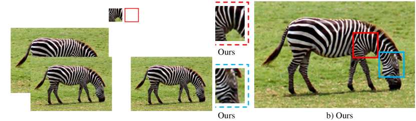
Figure 5: Qualitative results of our method against CutBlur [Yoo et al.(2020)Yoo, Ahn, and Sohn].

method	PSNR	gain
Baseline	34.56
ours 0.1	34.68	+0.12
ours 0.3	34.68	+0.12
ours 0.5	34.67	+0.11
PatchNet	34.65	+0.09
OHEM 0.1	34.39	-0.17
OHEM 0.3	34.56	-0.01
OHEM 0.5	34.62	+0.06

Table 6: Comparison with PatchNet and Online Hard example Mining (OHEM). The PSNR results of EDSR are reported in DIV2K dataset at x2 scale. The decimal indicates the portion of dataset.

Ours		CutBlur
portion	PSNR	portion	PSNR
baseline	28.55	baseline	28.56
0.5	28.68 (+0.13)	0.9	28.29 (-0.27)
0.1	28.69 (+0.14)	0.5	28.39 (-0.17)
1e-6	28.62 (+0.07)	0.1	28.37 (-0.19)
0.5   + pre	28.93 (+0.38)	0.9 + pre	28.73 (+0.17)
0.1   + pre	28.90 (+0.35)	0.5 + pre	28.74 (+0.18)
1e-6 + pre	28.79 (+0.24)	0.1 + pre	28.73 (+0.17)

Table 7: Comparison of our method against CutBlur [Yoo et al.(2020)Yoo, Ahn, and Sohn]. The PSNR results of EDSR are reported in DIV2K dataset at x4 scale. $pre$ denotes pretraining.

We also compare our approach against two online sampling methods PatchNet [Sun et al.(2020)Sun, Chen, Slabaugh, and Torr] and OHEM [Shrivastava et al.(2016)Shrivastava, Gupta, and Girshick]. PatchNet trains an additional network to measure the trainability of each patch, and only uses the trainable patches during training. OHEM only back-propagates the highest losses in every training batch. We observe that OHEM is unstable to converge in SR training. As can be seen in Tab. 7, hard negative mining fails to achieve consistent performance improvement and our approach achieves better results compared with PatchNet. All the results show the effectiveness of our method.

5 Conclusion

In this paper, we study the data augmentation problem for SR in terms of patch sampling. we first devise a simple yet effective metric to measure the informative importance of LR-HR patch pairs. Then we propose an efficient solution based on integral image, which significantly reduces the computational cost of calculating this metric for every image. Instead of uniformly sampling all patches for SR training, we sample the most informative patches. Extensive experiments are conducted to validate the effectiveness and advantages of the proposed method across various architectures, scaling factors and datasets. We hope this paper can inspire future works on data augmentation for SR.

References

- [Agustsson and Timofte(2017)] Eirikur Agustsson and Radu Timofte. Ntire 2017 challenge on single image super-resolution: Dataset and study. In The IEEE Conference on Computer Vision and Pattern Recognition (CVPR) Workshops, July 2017.
- [Bako et al.(2017)Bako, Vogels, McWilliams, Meyer, Novák, Harvill, Sen, Derose, and Rousselle] Steve Bako, Thijs Vogels, Brian McWilliams, Mark Meyer, Jan Novák, Alex Harvill, Pradeep Sen, Tony Derose, and Fabrice Rousselle. Kernel-predicting convolutional networks for denoising monte carlo renderings. ACM Trans. Graph., 36(4):97–1, 2017.
- [Cai et al.(2019)Cai, Zeng, Yong, Cao, and Zhang] Jianrui Cai, Hui Zeng, Hongwei Yong, Zisheng Cao, and Lei Zhang. Toward real-world single image super-resolution: A new benchmark and a new model. In Proceedings of the IEEE/CVF International Conference on Computer Vision, pages 3086–3095, 2019.
- [Crow(1984)] Franklin C Crow. Summed-area tables for texture mapping. In Proceedings of the 11th annual conference on Computer graphics and interactive techniques, pages 207–212, 1984.
- [Dong et al.(2014)Dong, Loy, He, and Tang] Chao Dong, Chen Change Loy, Kaiming He, and Xiaoou Tang. Learning a deep convolutional network for image super-resolution. In European conference on computer vision, pages 184–199. Springer, 2014.
- [Dong et al.(2016)Dong, Loy, and Tang] Chao Dong, Chen Change Loy, and Xiaoou Tang. Accelerating the super-resolution convolutional neural network. In European conference on computer vision, pages 391–407. Springer, 2016.
- [Gharbi et al.(2016)Gharbi, Chaurasia, Paris, and Durand] Michaël Gharbi, Gaurav Chaurasia, Sylvain Paris, and Frédo Durand. Deep joint demosaicking and denoising. ACM Transactions on Graphics (TOG), 35(6):1–12, 2016.
- [Girshick(2015)] Ross Girshick. Fast r-cnn. In Proceedings of the IEEE international conference on computer vision, pages 1440–1448, 2015.
- [Hui et al.(2018)Hui, Wang, and Gao] Zheng Hui, Xiumei Wang, and Xinbo Gao. Fast and accurate single image super-resolution via information distillation network. In Proceedings of the IEEE conference on computer vision and pattern recognition, pages 723–731, 2018.
- [Kim et al.(2016)Kim, Kwon Lee, and Mu Lee] Jiwon Kim, Jung Kwon Lee, and Kyoung Mu Lee. Accurate image super-resolution using very deep convolutional networks. In Proceedings of the IEEE conference on computer vision and pattern recognition, pages 1646–1654, 2016.
- [Kong et al.(2021)Kong, Zhao, Qiao, and Dong] Xiangtao Kong, Hengyuan Zhao, Yu Qiao, and Chao Dong. Classsr: A general framework to accelerate super-resolution networks by data characteristic. arXiv preprint arXiv:2103.04039, 2021.
- [Ledig et al.(2017)Ledig, Theis, Huszár, Caballero, Cunningham, Acosta, Aitken, Tejani, Totz, Wang, et al.] Christian Ledig, Lucas Theis, Ferenc Huszár, Jose Caballero, Andrew Cunningham, Alejandro Acosta, Andrew Aitken, Alykhan Tejani, Johannes Totz, Zehan Wang, et al. Photo-realistic single image super-resolution using a generative adversarial network. In Proceedings of the IEEE conference on computer vision and pattern recognition, pages 4681–4690, 2017.
- [Li et al.(2020)Li, Zhou, Qi, Jiang, Lu, and Jia] Wenbo Li, Kun Zhou, Lu Qi, Nianjuan Jiang, Jiangbo Lu, and Jiaya Jia. Lapar: Linearly-assembled pixel-adaptive regression network for single image super-resolution and beyond. Advances in Neural Information Processing Systems, 33, 2020.
- [Lim et al.(2017)Lim, Son, Kim, Nah, and Mu Lee] Bee Lim, Sanghyun Son, Heewon Kim, Seungjun Nah, and Kyoung Mu Lee. Enhanced deep residual networks for single image super-resolution. In Proceedings of the IEEE conference on computer vision and pattern recognition workshops, pages 136–144, 2017.
- [Park et al.(2020)Park, Yoo, Cho, Kim, and Kim] Seobin Park, Jinsu Yoo, Donghyeon Cho, Jiwon Kim, and Tae Hyun Kim. Fast adaptation to super-resolution networks via meta-learning. arXiv preprint arXiv:2001.02905, 5, 2020.
- [Shaham et al.(2019)Shaham, Dekel, and Michaeli] Tamar Rott Shaham, Tali Dekel, and Tomer Michaeli. Singan: Learning a generative model from a single natural image. In Proceedings of the IEEE/CVF International Conference on Computer Vision, pages 4570–4580, 2019.
- [Shi et al.(2016)Shi, Caballero, Huszár, Totz, Aitken, Bishop, Rueckert, and Wang] Wenzhe Shi, Jose Caballero, Ferenc Huszár, Johannes Totz, Andrew P Aitken, Rob Bishop, Daniel Rueckert, and Zehan Wang. Real-time single image and video super-resolution using an efficient sub-pixel convolutional neural network. In Proceedings of the IEEE conference on computer vision and pattern recognition, pages 1874–1883, 2016.
- [Shocher et al.(2018)Shocher, Cohen, and Irani] Assaf Shocher, Nadav Cohen, and Michal Irani. “zero-shot” super-resolution using deep internal learning. In Proceedings of the IEEE Conference on Computer Vision and Pattern Recognition, pages 3118–3126, 2018.
- [Shrivastava et al.(2016)Shrivastava, Gupta, and Girshick] Abhinav Shrivastava, Abhinav Gupta, and Ross Girshick. Training region-based object detectors with online hard example mining. In Proceedings of the IEEE conference on computer vision and pattern recognition, pages 761–769, 2016.
- [Soh et al.(2020)Soh, Cho, and Cho] Jae Woong Soh, Sunwoo Cho, and Nam Ik Cho. Meta-transfer learning for zero-shot super-resolution. In Proceedings of the IEEE/CVF Conference on Computer Vision and Pattern Recognition, pages 3516–3525, 2020.
- [Sun et al.(2020)Sun, Chen, Slabaugh, and Torr] Shuyang Sun, Liang Chen, Gregory Slabaugh, and Philip Torr. Learning to sample the most useful training patches from images. arXiv preprint arXiv:2011.12097, 2020.
- [Xin et al.(2020)Xin, Wang, Jiang, Li, Huang, and Gao] Jingwei Xin, Nannan Wang, Xinrui Jiang, Jie Li, Heng Huang, and Xinbo Gao. Binarized neural network for single image super resolution. In European Conference on Computer Vision, pages 91–107. Springer, 2020.
- [Xu et al.(2019)Xu, Ma, and Sun] Xiangyu Xu, Yongrui Ma, and Wenxiu Sun. Towards real scene super-resolution with raw images. In Proceedings of the IEEE/CVF Conference on Computer Vision and Pattern Recognition, pages 1723–1731, 2019.
- [Yoo et al.(2020)Yoo, Ahn, and Sohn] Jaejun Yoo, Namhyuk Ahn, and Kyung-Ah Sohn. Rethinking data augmentation for image super-resolution: A comprehensive analysis and a new strategy. In Proceedings of the IEEE/CVF Conference on Computer Vision and Pattern Recognition, pages 8375–8384, 2020.
- [Yun et al.(2019)Yun, Han, Oh, Chun, Choe, and Yoo] Sangdoo Yun, Dongyoon Han, Seong Joon Oh, Sanghyuk Chun, Junsuk Choe, and Youngjoon Yoo. Cutmix: Regularization strategy to train strong classifiers with localizable features. In Proceedings of the IEEE/CVF International Conference on Computer Vision, pages 6023–6032, 2019.
- [Zhang et al.(2017)Zhang, Cisse, Dauphin, and Lopez-Paz] Hongyi Zhang, Moustapha Cisse, Yann N Dauphin, and David Lopez-Paz. mixup: Beyond empirical risk minimization. arXiv preprint arXiv:1710.09412, 2017.
- [Zhang et al.(2018a)Zhang, Li, Li, Wang, Zhong, and Fu] Yulun Zhang, Kunpeng Li, Kai Li, Lichen Wang, Bineng Zhong, and Yun Fu. Image super-resolution using very deep residual channel attention networks. In Proceedings of the European conference on computer vision (ECCV), pages 286–301, 2018a.
- [Zhang et al.(2018b)Zhang, Tian, Kong, Zhong, and Fu] Yulun Zhang, Yapeng Tian, Yu Kong, Bineng Zhong, and Yun Fu. Residual dense network for image super-resolution. In Proceedings of the IEEE conference on computer vision and pattern recognition, pages 2472–2481, 2018b.